Dual Moments and Risk Attitudes

Abstract

In decision under risk, the primal moments of mean and variance play a central role to define the local index of absolute risk aversion. In this paper, we show that in canonical non-EU models dual moments have to be used instead of, or on par with, their primal counterparts to obtain an equivalent index of absolute risk aversion.
Keywords: Risk Premium; Expected Utility; Dual Theory; Rank-Dependent Utility; Local Index; Absolute Risk Aversion.
JEL Classification: D81.
OR/MS Classification: Decision analysis: Risk.

1 Introduction

In their important seminal work, Pratt P64 and Arrow A65 , A71 (henceforth, PA) show that under expected utility (EU) the risk premium $\pi$ associated to a small risk $\tilde{\varepsilon}$ with zero mean can be approximated by the following expression:

$$\pi\simeq\frac{\texttt{m}_{2}}{2}\left(-\frac{U^{\prime\prime}(w_{0})}{U^{\prime}(w_{0})}\right).$$ (1.1)

Here, $\texttt{m}_{2}$ is the second moment about the mean (i.e., the variance) of $\tilde{\varepsilon}$ while $U^{\prime}(w_{0})$ and $U^{\prime\prime}(w_{0})$ are the first and second derivatives of the utility function of wealth $U$ at the initial wealth level $w_{0}$. In the PA-approach, the designation “small” refers to a risk that has a probability mass equal to unity but a small variance. The PA-approximation in (1.1) provides a very insightful dissection of the EU risk premium, disentangling the complex interplay between the probability distribution of the risk, the decision-maker’s risk attitude, and his initial wealth. This well-known result has led to many developments and applications within the EU model in many fields.

The aim of this paper is to show that a similar result can also be obtained outside EU, in the dual theory of choice under risk (DT; Yaari Y87 ) and, more generally and behaviorally more relevant, under rank-dependent utility (RDU; Quiggin Q82 ). To achieve this, we substitute or complement the primal second moment $\texttt{m}_{2}$ by its dual counterpart, and substitute or complement the derivatives of the utility function $U$ by the respective derivatives of the probability weighting function.^, This modification enables us to develop for these two canonical non-EU models a simple and intuitive local index of risk attitude that resembles the one in (1.1) under EU. Our results allow for quite arbitrary utility and probability weighting functions including inverse $s$-shaped functions such as the probability weighting functions in Prelec P98 and Wu and Gonzalez WG96 , which are descriptively relevant (Abdellaoui A00 ). Thus, we allow for violations of strong risk aversion (Chew, Karni and Safra CKS87 and Roëll R87 ) in the sense of aversion to mean-preserving spreads à la Rothschild and Stiglitz RS70 (see also Machina and Pratt MP97 ).^,

Our paper is organized as follows. In Section 2 we define the second dual moment and we use it in Section 3 to develop the local index of absolute risk aversion under DT. In Section 4 we extend our results to the RDU model. Section 5 discusses related literature and Section 6 illustrates our results in examples. In Section 7 we present an application to portfolio choice and we provide a conclusion in Section 8. Some supplementary material, including some technical details to supplement Sections 3 and 4, the proof of a result in Section 5, and two illustrations to supplement Section 6, suppressed in this version to save space, is contained in an online appendix.

2 The Second Dual Moment

The second dual moment about the mean of an arbitrary risk $\tilde{\varepsilon}$, denoted by $\bar{\texttt{m}}_{2}$, is defined by

$$\bar{\texttt{m}}_{2}:=\mathbb{E}\left[\max\left(\tilde{\varepsilon}^{(1)},\tilde{\varepsilon}^{(2)}\right)\right]-\mathbb{E}\left[\tilde{\varepsilon}\right],$$ (2.1)

where $\tilde{\varepsilon}^{(1)}$ and $\tilde{\varepsilon}^{(2)}$ are two independent copies of $\tilde{\varepsilon}$. The second dual moment can be interpreted as the expectation of the largest order statistic: it represents the expected best outcome among two independent draws of the risk.

Our analysis will reveal that for an RDU maximizer who evaluates a small zero-mean risk, the second dual moment stands on equal footing with the variance as a fundamental measure of risk. While the variance provides a measure of risk in the “payoff plane”, the second dual moment can be thought of as a measure of risk in the “probability plane”. Indeed, for a risk $\tilde{\varepsilon}$ with cumulative distribution function $F$, so

$$\texttt{m}:=\mathbb{E}\left[\tilde{\varepsilon}\right]=\int x\,\mathrm{d}F(x),$$

we have that

$$\texttt{m}_{2}=\int(x-\texttt{m})^{2}\,\mathrm{d}F(x),\qquad\mathrm{while}\qquad\bar{\texttt{m}}_{2}=\int(x-\texttt{m})\,\mathrm{d}(F(x))^{2}.$$

For the sake of brevity and in view of (2.1), we shall term the second dual moment about the mean, $\bar{\texttt{m}}_{2}$, the maxiance by analogy to the variance. Our designation “small” in “small zero-mean risk” will quite naturally refer to a risk with small maxiance under DT and to a risk with both small variance and small maxiance under RDU.

One readily verifies that for a zero-mean risk $\tilde{\varepsilon}$,

$$\mathbb{E}\left[\max\left(\tilde{\varepsilon}^{(1)},\tilde{\varepsilon}^{(2)}\right)\right]=-\mathbb{E}\left[\min\left(\tilde{\varepsilon}^{(1)},\tilde{\varepsilon}^{(2)}\right)\right].$$

The miniance—the expected worst outcome among two independent draws—is perhaps a more natural measure of “risk”, but agrees with the maxiance for zero-mean risks upon a sign change.

Just like the first and second primal moments occur under EU when the utility function is linear and quadratic, the first and second dual moments correspond to a linear and quadratic probability weighting function under DT. For further details on mean order statistics and their integral representations we refer to David D81 . In the stochastic dominance literature, these expectations of order statistics and their higher-order generalizations arise naturally in an interesting paper by Muliere and Scarsini MS89 , when defining a sequence of progressive $n$-th degree “inverse” stochastic dominances by analogy to the conventional stochastic dominance sequence (see Ekern E80 and Fishburn F80 ).^,

3 Local Risk Aversion under the Dual Theory

Consider a DT decision-maker. His evaluation of a risk $A$ with cumulative distribution function $F$ is given by

$$\int x\,\mathrm{d}h\left(F(x)\right),$$ (3.1)

where the probability weighting (distortion) function $h:[0,1]\rightarrow[0,1]$ satisfies the usual properties ($h(0)=0$, $h(1)=1$, $h^{\prime}(p)>0$).^,

In order to develop the local index of absolute risk aversion under DT we start from a lottery $A$ given by the following representation:^,

Figure 1: Lottery $A$

We transform lottery $A$ into a lottery $B$ given by:

Figure 2: Lottery $B$

To obtain $B$ from $A$ we subtract a probability $\varepsilon_{1}$ from the probabilities of both states of the world in $A$ without changing the outcomes and we assign these two probabilities jointly, i.e., $2\varepsilon_{1}$, to a new intermediate state to which we attach an outcome $x$ with $-1<x<1$. If $x\equiv 0$, then $\mathbb{E}\left[A\right]=\mathbb{E}\left[B\right]$ and $B$ is a mean-preserving contraction of $A$.

The value of $x$ will be chosen such that the decision-maker is indifferent between $A$ and $B$. Naturally the difference between $0$ and $x$, denoted by $\rho=0-x$, represents the risk premium associated to the risk change from $A$ to $B$. As we will show in Section 5.2 this definition of the risk premium can be viewed as a natural generalization of the PA risk premium to the case of risk changes with probability mass less than unity. Depending on the shape of $h$ the risk premium $\rho$ may be positive or negative. If (and only if) $h^{\prime\prime}(p)<0$, the corresponding DT maximizer is averse to mean-preserving spreads, and would universally prefer $B$ over $A$ when $x$ were $0$. Thus, to establish indifference between $A$ and $B$ for such a decision-maker, $x$ has to be smaller than $0$, in which case $\rho$ is positive.

In general, for $x\equiv 0-\rho$ in $B$, indifference between $A$ and $B$ implies:

$$h\left(p_{0}\right)(w_{0}-1)+\left(1-h\left(p_{0}\right)\right)(w_{0}+1)$$ (3.2)

$$=h\left(p_{0}-\varepsilon_{1}\right)(w_{0}-1)+\left(h\left(p_{0}+\varepsilon_{1}\right)-h\left(p_{0}-\varepsilon_{1}\right)\right)\left(w_{0}-\rho\right)+\left(1-h\left(p_{0}+\varepsilon_{1}\right)\right)(w_{0}+1),$$

where $w_{0}$ is the decision-maker’s initial wealth level. From (3.2) we obtain the explicit solution

$$\rho=\frac{\left(h\left(p_{0}\right)-h\left(p_{0}-\varepsilon_{1}\right)\right)-\left(h\left(p_{0}+\varepsilon_{1}\right)-h\left(p_{0}\right)\right)}{\left(h\left(p_{0}+\varepsilon_{1}\right)-h\left(p_{0}-\varepsilon_{1}\right)\right)}.$$ (3.3)

By approximating $h\left(p_{0}\pm\varepsilon_{1}\right)$ in (3.3) using second-order Taylor series expansions around $h(p_{0})$, we obtain the following approximation for the DT risk premium:

$$\rho\simeq\frac{\bar{\texttt{m}}_{2}}{2\texttt{Pr}}\left(-\frac{h^{\prime\prime}(p_{0})}{h^{\prime}(p_{0})}\right).$$ (3.4)

Here, $\bar{\texttt{m}}_{2}$ is the unconditional maxiance of the risk $\tilde{\varepsilon}_{1}$ that describes the mean-preserving spread from $B$ with $x\equiv 0$ to $A$. Unconditionally, $\tilde{\varepsilon}_{1}$ takes the values $\pm 1$ each with probability $\varepsilon_{1}$. Furthermore, Pr is the total unconditional probability mass associated to $\tilde{\varepsilon}_{1}$; see Figure 3.

Figure 3: Mean-Preserving Spread from $B$ with $x\equiv 0$ to $A$.

Observe that lottery $A$ is obtained from lottery $B$ (with $x\equiv 0$) by attaching the risk $\tilde{\varepsilon}_{1}$ to the intermediate branch of $B$. That is, the risk $\tilde{\varepsilon}_{1}$ is effective conditionally upon realization of the intermediate state of lottery $B$, which occurs with probability $2\varepsilon_{1}$. One readily verifies that, for this risk $\tilde{\varepsilon}_{1}$, we have that, unconditionally, $\bar{\texttt{m}}_{2}=2\varepsilon_{1}^{2}$ and $\texttt{Pr}=2\varepsilon_{1}$. We consider the unconditional maxiance of the zero-mean risk $\tilde{\varepsilon}_{1}$ to be “small” and compute the Taylor expansions up to the order $\varepsilon_{1}^{2}$. Henceforth, maxiances and variances are always understood to be unconditional.

It is important to compare the result in (3.4) to that obtained by PA presented in (1.1). In PA the local approximation of the risk premium is proportional to the variance, while under DT it is proportional to the maxiance.

We note that the local approximation of the risk premium in (3.4) remains valid in general, for non-binary zero-mean risks $\tilde{\varepsilon}_{1}$ with small maxiance, just like, as is well-known, (1.1) is valid for non-binary zero-mean risks with small variance.

4 Local Risk Aversion under Rank-Dependent Utility

Under DT the local index arises from a risk change with small maxiance. To deal with the RDU model, which encompasses both EU and DT as special cases, we naturally have to consider changes in risk that are small in both variance and maxiance. To achieve this, we start from a lottery $C$ given by:

Figure 4: Lottery $C$

Similar to under DT, we transform lottery $C$ into a lottery $D$ by reducing the probabilities of both states in $C$ by a probability $\varepsilon_{1}$ and assigning the released probability $2\varepsilon_{1}$ to an intermediate state with outcome $y$, where $-\varepsilon_{2}<y<\varepsilon_{2}$. This yields a lottery $D$ given by:

Figure 5: Lottery $D$

Of course, when $y\equiv 0$, $D$ is a mean-preserving contraction of $C$. All RDU decision-makers that are averse to mean-preserving spreads therefore prefer $D$ over $C$ in that case. Formally, an RDU decision-maker evaluates a lottery $A$ with cumulative distribution function $F$ by computing

$$\int U(x)\,\mathrm{d}h\left(F(x)\right),$$ (4.1)

and is averse to mean-preserving spreads if and only if $U^{\prime\prime}<0$ and $h^{\prime\prime}<0$.

In general, we can search for $y$ such that indifference between $C$ and $D$ occurs. The discrepancy between the resulting $y$ and $0$ is the RDU risk premium associated to the risk change from $C$ to $D$ and its value, denoted by $\lambda=0-y$, is the solution to

$$h\left(p_{0}\right)U\left(w_{0}-\varepsilon_{2}\right)+\left(1-h\left(p_{0}\right)\right)U\left(w_{0}+\varepsilon_{2}\right)$$ (4.2)

$$\hskip-2.84544pt=\ h\left(p_{0}-\varepsilon_{1}\right)U\left(w_{0}-\varepsilon_{2}\right)+\left(h\left(p_{0}+\varepsilon_{1}\right)-h\left(p_{0}-\varepsilon_{1}\right)\right)U\left(w_{0}-\lambda\right)+\left(1-h\left(p_{0}+\varepsilon_{1}\right)\right)U\left(w_{0}+\varepsilon_{2}\right).$$

It will be positive or negative depending on the shapes of $U$ and $h$.

Approximating the solution to (4.2) by Taylor series expansions, up to the first order in $\lambda$ around $U\left(w_{0}\right)$ and up to the second orders in $\varepsilon_{1}$ and $\varepsilon_{2}$ around $U\left(w_{0}\right)$ and $h\left(p_{0}\right)$, we obtain the following approximation for the RDU risk premium:

$$\lambda\simeq\frac{\texttt{m}_{2}}{2\texttt{Pr}}\left(-\frac{U^{\prime\prime}(w_{0})}{U^{\prime}(w_{0})}\right)+\frac{\bar{\texttt{m}}_{2}}{2\texttt{Pr}}\left(-\frac{h^{\prime\prime}(p_{0})}{h^{\prime}(p_{0})}\right).$$ (4.3)

Here, $\texttt{m}_{2}$ and $\bar{\texttt{m}}_{2}$ are the unconditional variance and maxiance of the risk $\tilde{\varepsilon}_{12}$ that dictates the mean-preserving spread from $D$ with $y\equiv 0$ to $C$. Unconditionally, $\tilde{\varepsilon}_{12}$ takes the values $\pm\varepsilon_{2}$ each with probability $\varepsilon_{1}$. Furthermore, Pr is the total unconditional probability mass associated to $\tilde{\varepsilon}_{12}$.

Comparing (4.3) to (1.1) and (3.4) reveals that the local approximation of the RDU risk premium aggregates the (suitably scaled) EU and DT counterparts, with the variance and maxiance featuring equally prominently.

As shown in online supplementary material, the local approximation of the RDU risk premium in (4.3) also generalizes naturally to non-binary risks $\tilde{\varepsilon}_{12}$.

5 Related Literature

5.1 Global Results: Comparative Risk Aversion under RDU

Not only the local properties of the previous sections are valid under DT and RDU but also the corresponding global properties, just like in the PA-approach under the EU model (see, in particular, Theorem 1 in Pratt P64 ). In this section, we restrict attention to the RDU model. (The DT model occurs as a special case.) We first note that the definition of the RDU risk premium in (4.2) applies also when $\varepsilon_{1}$ and $\varepsilon_{2}$ are “large”, as long as $0<\varepsilon_{1}\leq\{p_{0},1-p_{0}\}<1$ and $\varepsilon_{2}>0$ are satisfied. We then state the following result:

Proposition 5.1

Let $U_{i}$, $h_{i}$, $\lambda_{i}(p_{0},w_{0},\varepsilon_{1},\varepsilon_{2})$ be the utility function, the probability weighting function, and the risk premium solving (4.2) for RDU decision-maker $i=1,2$. Then the following conditions are equivalent:

• $-\frac{U_{2}^{\prime\prime}(w)}{U_{2}^{\prime}(w)}\geq-\frac{U_{1}^{\prime\prime}(w)}{U_{1}^{\prime}(w)}$ and $-\frac{h_{2}^{\prime\prime}(p)}{h_{2}^{\prime}(p)}\geq-\frac{h_{1}^{\prime\prime}(p)}{h_{1}^{\prime}(p)}$     for all $w$ and all $p\in(0,1)$.

• $\lambda_{2}(p_{0},w_{0},\varepsilon_{1},\varepsilon_{2})\geq\lambda_{1}(p_{0},w_{0},\varepsilon_{1},\varepsilon_{2})$     for all $0<\varepsilon_{1}\leq\{p_{0},1-p_{0}\}<1$, all $w_{0}$, and all $\varepsilon_{2}>0$.

Because the binary symmetric zero-mean risk $\tilde{\varepsilon}_{12}$ in Section 4 induces a risk change that is a special case of a mean-preserving spread, the implication (i)$\Rightarrow$(ii) in Proposition 5.1 in principle follows from the classical results on comparative risk aversion under RDU (Yaari Y86 , Chew, Karni and Safra CKS87 , and Roëll R87 ). The reverse implication (ii)$\Rightarrow$(i) formalizes the connection between our local risk aversion approach and global risk aversion under RDU.

Due to the simultaneous involvement of both the utility function and the probability weighting function, the proof of the equivalences between (i) and (ii) under RDU is more complicated than that of the analogous properties under EU (and DT). Our proof of Proposition 5.1 (which is contained in online supplementary material available from the authors’ webpages) is based on the total differential of the RDU evaluation, and the sensitivity of the risk premium with respect to changes in payoffs.

5.2 Relation to the Pratt-Arrow Definition of the Risk Premium

Our definition of the risk premium under RDU in (4.2) can be viewed as a natural generalization of the risk premium of Pratt P64 and Arrow A65 , A71 . To see this, first note that the PA-definition, under which a risk is compared to a sure loss equal to the risk premium, occurs when $p_{0}=\varepsilon_{1}=\frac{1}{2}$. Then, lottery $D$ becomes a sure loss of $\lambda$ the value of which is such that the decision-maker is indifferent to the risk of lottery $C$.

When $\varepsilon_{1}<\frac{1}{2}$, our definition of the RDU risk premium provides a natural generalization of the PA-definition. This becomes readily apparent if we omit the common components of lotteries $D$ and $C$ with the same incremental RDU evaluation and isolate the risk change, which yields

Figure 6: Lottery $D$ after Omitting the Components in Common with Lottery $C$.

and

Figure 7: Lottery $C$ after Omitting the Components in Common with Lottery $D$.

The value of $\lambda$ thus represents the risk premium for the risk change induced by a risk that, unconditionally, takes the values $\pm\varepsilon_{2}$ each with probability $\varepsilon_{1}$.

When $\varepsilon_{1}<\frac{1}{2}$, the original comparison between $C$ and $D$ is a comparison between two risky situations as in Ross R81 , Machina and Neilson MN87 , and Pratt P90 . The removal of common components, however, reveals that we essentially face a PA-comparison between a single loss and a risk with the same total probability mass, which is now allowed to be smaller than unity.

5.3 Related Measures of Risk

Dual moments can be related to the Gini cofficient named after statistician Corrado Gini and used by economists to measure the dispersion of the income distribution of a population, summarizing its income inequality. In risk theory, the Gini coefficient $\mathcal{G}$ of a risk $A$ is usually defined by

$$\mathcal{G}=\frac{\mathbb{E}\left[|A^{(1)}-A^{(2)}|\right]}{2\mathbb{E}\left[A\right]},$$ (5.4)

which represents half the relative (i.e., normalized) expected absolute difference between two independent draws of the risk $A$. One can verify that, equivalently but less well-known,

$$\mathcal{G}=\frac{\bar{\texttt{m}}_{2}}{\texttt{m}}.$$ (5.5)

This alternative expression features the ratio of the maxiance and the first moment.

Furthermore, $n$-th degree expectations of first order statistics also appear in Cherny and Madan CM09 as performance measures in the context of portfolio evaluation. In this setting, the expected maximal financial loss occurring in $n$ independent draws of a risk is used as a measure to define an acceptability index linked to a tolerance level of stress.

6 Examples

Owing to its local nature, our approximation is valid and can insightfully be applied when the probability weighting function is not globally concave, as is suggested by ample experimental evidence. Consider the canonical probability weighting function of Prelec P98 given by

$$h(p)=1-\exp\left\{-\left(-\log\left(1-p\right)\right)^{\alpha}\right\},\qquad 0<\alpha<1.$$ (6.1)

It captures the following properties which are observed empirically: it is regressive (first, $h(p)>p$, next $h(p)<p$), is inverse $s$-shaped (first concave, next convex), and is asymmetric (intersecting the identity probability weighting function $h(p)=p$ at $p^{*}=1-1/\exp(1)$, the inflection point). The upper panel of Figure 8 plots this probability weighting function for $\alpha\in\{0.1,0.3,\ldots,0.9\}$. (Wu and Gonzalez WG96 report estimated values of $\alpha$ between 0.03 and 0.95.)

Its local index $-\frac{h^{\prime\prime}(p)}{h^{\prime}(p)}$ takes the form

$$-\frac{h^{\prime\prime}(p)}{h^{\prime}(p)}=-\frac{1-\alpha\left(1-\left(-\log(1-p)\right)^{\alpha}\right)+\log(1-p)}{(1-p)\log(1-p)}.$$ (6.2)

Figure 8, lower panel, plots this local index for $\alpha\in\{0.1,0.3,\ldots,0.9\}$.

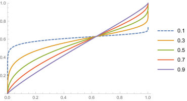
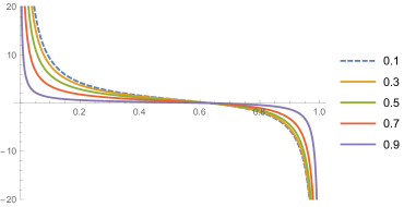
Figure 8: Prelec’s Probability Weighting Function (upper panel) and its Local Index (lower panel). We consider $\alpha\in\{0.1,0.3,\ldots,0.9\}$.

The inverse $s$-shape of the probability weighting function (first concave, next convex) implies that its local index changes sign at the inflection point. More specifically, the local index associated with Prelec’s probability weighting function is decreasing (first positive, next negative) in $p$ for any $0<\alpha<1$. This property is naturally consistent with the inverse $s$-shape property of the probability weighting function: the inverse $s$-shape property is meant to represent a psychological phenomenon known as diminishing sensitivity in the probability domain (rather than the payoff domain), under which the decision-maker is less sensitive to changes in the objective probabilities when they move away from the reference points $0$ and $1$, and becomes more sensitive when the objective probabilities move towards these reference points.

A decreasing local index implies in particular that $h^{\prime\prime\prime}>0$. (By Pratt P64 , the sign of the derivative of the local index is the same as the sign of $\left(h^{\prime\prime}(p)\right)^{2}-h^{\prime}(p)h^{\prime\prime\prime}(p)$.) Inverse $s$-shaped probability weighting functions, including Prelec’s canonical example, usually exhibit positive signs for the odd derivatives and alternating signs (first negative, then positive) for the even derivatives. For a probability weighting function that is inverse $s$-shaped (first concave, then convex) and has second derivative equal to zero at the inflection point, a positive sign of the third derivative means that the function becomes increasingly concave when we move to the left of the inflection point and becomes increasingly convex when we move to the right of the inflection point.

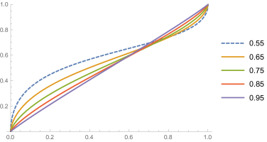
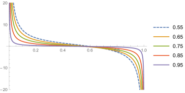
Figure 12: Tversky-Kahneman Probability Weighting Function (upper panel) and its Local Index (lower panel). We consider $\beta\in\{0.55,0.65,\ldots,0.95\}$.

In Figure 12 in the online appendix we also plot the local index $-\frac{h^{\prime\prime}(p)}{h^{\prime}(p)}$ of the probability weighting function proposed by Tversky and Kahneman TK92 (see also Wu and Gonzalez WG96 ) given by

$$h(p)=1-\frac{\left(1-p\right)^{\beta}}{\left(\left(1-p\right)^{\beta}+p^{\beta}\right)^{1/\beta}},\qquad 0<\beta<1,$$ (6.3)

for values of the parameter $\beta\in\{0.55,0.65,\ldots,0.95\}$ as found in experiments (Wu and Gonzalez WG96 report estimated values of $\beta$ between 0.57 and 0.94). Observe the similarity between the shapes in Figure 8 and Figure 12.

The analysis in this paper reveals that for a small risk the sign and size of the maxiance’s contribution to the RDU risk premium, given by the second term on the right-hand side of (4.3), i.e.,

$$\frac{\bar{\texttt{m}}_{2}}{2\texttt{Pr}}\left(-\frac{h^{\prime\prime}(p_{0})}{h^{\prime}(p_{0})}\right),$$

varies with the probability level $p_{0}$, from strongly positive to strongly negative, in tandem with the local index $-\frac{h^{\prime\prime}(p)}{h^{\prime}(p)}$ to which it is proportional.

We finally plot in Figure 9 our approximation to the RDU risk premium (4.3) of a risk with small variance and maxiance normalized to satisfy $\frac{\texttt{m}_{2}}{2\texttt{Pr}}=\frac{\bar{\texttt{m}}_{2}}{2\texttt{Pr}}=1$, as a function of both the initial wealth level $w_{0}$ and the probability level $p_{0}$. We suppose the utility function is given by the conventional power utility (note that we consider a pure rank-dependent model)

$$U(x)=x^{\gamma},$$

with $\gamma=0.5$ (consistent with the gain domain in Tversky and Kahneman TK92 and with experimental evidence in Wu and Gonzalez WG96 ), and the probability weighting function is that of Prelec with parameter $\alpha=0.65$.

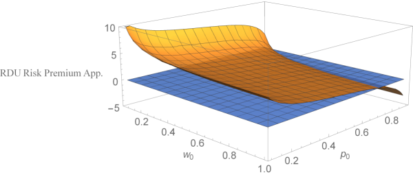
Figure 9: Surface of the RDU Risk Premium Approximation. We consider a risk with small variance and maxiance normalized to satisfy $\frac{\texttt{m}_{2}}{2\texttt{Pr}}=\frac{\bar{\texttt{m}}_{2}}{2\texttt{Pr}}=1$ under power utility (with $\gamma=0.5$) and Prelec’s probability weighting function (with $\alpha=0.65$).

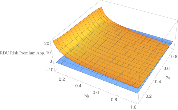
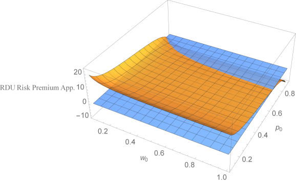
Figure 13: Surface of the RDU Risk Premium Approximation. We consider a risk with small variance and maxiance, normalized to satisfy $\frac{\bar{\texttt{m}}_{2}}{2\texttt{Pr}}=1$ with $\texttt{m}_{2}/\bar{\texttt{m}}_{2}=3$ (upper panel) and $\frac{\texttt{m}_{2}}{2\texttt{Pr}}=1$ with $\texttt{m}_{2}/\bar{\texttt{m}}_{2}=1/3$ (lower panel), under power utility (with $\gamma=0.5$) and Prelec’s probability weighting function (with $\alpha=0.65$).

Figure 9 illustrates the interplay between the variance’s and the maxiance’s contributions to the RDU risk premium (4.3), depending on the local indices $\left(-\frac{U^{\prime\prime}(w)}{U^{\prime}(w)}\right)$ and $\left(-\frac{h^{\prime\prime}(p)}{h^{\prime}(p)}\right)$ evaluated in the wealth and probability levels $w_{0}$ and $p_{0}$, respectively. The orange surface represents our approximation (4.3) to the RDU risk premium $\lambda$, while the blue surface is the $\lambda=0$-plane. To illustrate the effect of a change in variance or maxiance, we also plot in Figure 13 in the online appendix the surface of the RDU risk premium approximation (4.3) for a small risk with ratio between the variance and maxiance equal to $3$ (upper panel) and $1/3$ (lower) panel, instead of a ratio of $1$ as in Figure 9.

7 A Portfolio Application

In order to illustrate how the concepts we have developed can be used we consider a simple portfolio problem with a safe asset, the return of which is zero, and a binary risky asset with returns expressed by the following representation:

Figure 10: Return Distribution of the Risky Asset

Taking $\frac{R_{1}}{R_{0}+R_{1}}>p_{0}$ makes the expected return strictly positive.

If an RDU investor has initial wealth $w_{0}$ his portfolio optimization problem is given by

$$\operatorname{arg\,max}_{\alpha}\left\{h\left(p_{0}\right)U\left(w_{0}-\alpha R_{0}\right)+\left(1-h\left(p_{0}\right)\right)U\left(w_{0}+\alpha R_{1}\right)\right\},$$ (7.1)

with first-order condition (FOC) given by

$$-R_{0}h\left(p_{0}\right)U^{\prime}\left(w_{0}-\alpha R_{0}\right)+R_{1}\left(1-h\left(p_{0}\right)\right)U^{\prime}\left(w_{0}+\alpha R_{1}\right)\equiv 0.$$

It is straightforward to show that the second-order condition for a maximum is satisfied provided $U^{\prime\prime}<0$.

Let us now pay attention to the RDU investor for whom it is optimal to choose not to invest in the risky asset, i.e., to select $\alpha\equiv 0$. Plugging $\alpha\equiv 0$ into the FOC we obtain the condition

$$h\left(p_{0}\right)\equiv\frac{R_{1}}{R_{0}+R_{1}}.$$ (7.2)

Without surprise, $h\left(p_{0}\right)>p_{0}$. This value of $h\left(p_{0}\right)$ expresses the intensity of risk aversion that induces the choice of $\alpha\equiv 0$.

Now consider a mean-preserving contraction of the return of the risky asset given by:

Figure 11: Mean-Preserving Contraction of the Risky Asset

One may verify that such a mean-preserving contraction for a decision-maker who had decided not to participate in the risky asset may induce him to select a strictly positive $\alpha$.

Hence, we raise the following question: By how much should we reduce the intermediate return $\frac{R_{1}-R_{0}}{2}$ to induce the decision-maker to stick to the optimal $\alpha$ equal to zero? The answer to this question is denoted by $\varsigma$.

Because we are concentrating on the situation where $\alpha\equiv 0$ is optimal, the analysis is related only to the shape of the probability weighting function. Indeed, the shape of $U$ that appears in the FOC through different values of $U^{\prime}$ becomes irrelevant at $\alpha\equiv 0$. The reason to concentrate on $\alpha\equiv 0$ where only the probability weighting function matters under RDU pertains to the well-known fact that under EU a mean-preserving contraction of the risky return has an ambiguous effect on the optimal $\alpha$ (Gollier G95 ).

It turns out that, upon invoking Taylor series expansions and after several basic manipulations, the reduction $\varsigma$ that answers our question raised above is given by

$$\varsigma\simeq\frac{\bar{\texttt{m}}_{2}}{2\texttt{Pr}}\left(-\frac{h^{\prime\prime}\left(p_{0}\right)}{h^{\prime}\left(p_{0}\right)}\right),$$ (7.3)

where $\bar{\texttt{m}}_{2}$ is the maxiance of the risk that, unconditionally, takes the values $\pm\frac{R_{0}+R_{1}}{2}$ each with probability $\varepsilon_{1}$, and where Pr is the total probability mass of this risk. Again the second dual moment (instead of the primal one) appears, jointly with the intensity of risk aversion induced by the probability weighting function. In particular, the mean-preserving contraction is an improvement and has made the risky asset attractive if and only of $\varsigma$ is positive.

8 Conclusion

Under EU, the risk premium is approximated by an expression that multiplies half the variance of the risk (i.e., its primal second central moment) by the local index of absolute risk aversion. This expression dissects the complex interplay between the risk’s probability distribution, the decision-maker’s preferences and his initial wealth that the risk premium in general depends on. Surprisingly, a similar expression almost never appears in non-EU models.

In this paper, we have shown that when one refers to the second dual moment—instead of, or on par with, the primal one—one obtains quite naturally an approximation of the risk premium in canonical non-EU models that mimics the one obtained within the EU model.

The PA-approximation of the risk premium under EU has induced thousands of applications and results in many fields such as operations research, insurance, finance, and environmental economics. So far, comparable developments have been witnessed to a much lesser extent outside the EU model. Hopefully, the new and simple expression of the approximated risk premium may contribute to a widespread analysis and use of risk premia for non-EU.

SUPPLEMENTARY MATERIAL
(FOR ONLINE PUBLICATION)

Appendix A Generalization to Non-Binary Risks

In this supplementary material, we first show that the local approximation for the DT risk premium in (3.4) remains valid for non-binary risks with small maxiance. Next, we prove that the RDU risk premium approximation in (4.3) also remains valid for non-binary risks with both small variance and small maxiance. Throughout this supplement, we consider $n$-state risks with probabilities $p_{i}$ associated to outcomes $x_{i}$, $i=1,\ldots,n$, with $n\in\mathbb{N}_{>0}$. We order states from the lowest outcome state (designated by state number 1) to the highest outcome state (designated by state number $n$), which means that $x_{1}\leq\cdots\leq x_{n}$.

We analyze the DT risk premium for a risk with $n\geq 2$ effective states that have equal unconditional probability of occurrence given by $\frac{2\varepsilon_{1}}{n}$, $0<\varepsilon_{1}\leq\frac{1}{2}$. The outcomes are, however, allowed to be the same among adjacent states; this would correspond to a risk with non-equal state probabilities. Note the generality provided by this construction. We suppose that the risk has mean equal to zero, so $\sum_{i=1}^{n}x_{i}=0$. One may verify that the unconditional maxiance of this $n$-state risk is given by

$$\bar{\texttt{m}}_{2}=\frac{4\varepsilon_{1}^{2}}{n^{2}}\sum_{i=1}^{n}\left(2i-1\right)x_{i},$$ (A.1)

and that the total probability mass $\texttt{Pr}=2\varepsilon_{1}$. Observe that the maxiance is of the order $\varepsilon_{1}^{2}$, i.e., $\bar{\texttt{m}}_{2}=O\left(\varepsilon_{1}^{2}\right)$.

Similar to the main text, this zero-mean risk is attached to the intermediate branch of lottery $B$ (with $x\equiv 0$) to induce a mean-preserving spread. (We normalize the outcomes of the zero-mean risk by restricting them to the interval $[-1,1]$. This ensures that the initial ordering of outcomes in lottery $B$ is not affected and can easily be generalized.) The DT risk premium $\rho$ then occurs as the solution to

$$\left(h\left(p_{0}+\varepsilon_{1}\right)-h\left(p_{0}-\varepsilon_{1}\right)\right)\left(w_{0}-\rho\right)$$

$$=\sum_{i=1}^{n}\left(h\left(p_{0}-\varepsilon_{1}+i\frac{2\varepsilon_{1}}{n}\right)-h\left(p_{0}-\varepsilon_{1}+\left(i-1\right)\frac{2\varepsilon_{1}}{n}\right)\right)\left(w_{0}+x_{i}\right).$$ (A.2)

From (A.2) we obtain the explicit solution

$$\rho=-\sum_{i=1}^{n}\frac{\left(h\left(p_{0}-\varepsilon_{1}+i\frac{2\varepsilon_{1}}{n}\right)-h\left(p_{0}-\varepsilon_{1}+\left(i-1\right)\frac{2\varepsilon_{1}}{n}\right)\right)}{h\left(p_{0}+\varepsilon_{1}\right)-h\left(p_{0}-\varepsilon_{1}\right)}x_{i}.$$ (A.3)

By invoking Taylor series expansions around $h\left(p_{0}\right)$ up to the second order in $\varepsilon_{1}$ we obtain from (A.3) the following approximation for the DT risk premium:

$$\rho \simeq-\sum_{i=1}^{n}\frac{\frac{1}{2}\left(2i-1\right)\frac{4\varepsilon_{1}^{2}}{n^{2}}h^{\prime\prime}\left(p_{0}\right)}{2\varepsilon_{1}h^{\prime}\left(p_{0}\right)}x_{i}$$

$$=\frac{\bar{\texttt{m}}_{2}}{2\texttt{Pr}}\left(-\frac{h^{\prime\prime}(p_{0})}{h^{\prime}(p_{0})}\right),$$

where the last equality follows directly from (A.1).

Finally, turning to the risk premium under RDU, we consider, as under DT, an $n$-state zero-mean risk with unconditional state probabilities $\frac{2\varepsilon_{1}}{n}$, so $\sum_{i=1}^{n}x_{i}=0$ and $\texttt{Pr}=2\varepsilon_{1}$, now assumed to satisfy additionally that $\texttt{m}_{2}=\frac{1}{n}\sum_{i=1}^{n}x_{i}^{2}=O\left(\varepsilon_{2}^{2}\right)$ for some $\varepsilon_{2}>0$. Upon attaching this zero-mean risk to the intermediate branch of lottery $D$ (with $y\equiv 0$ and assuming without losing generality that $|x_{i}|<\varepsilon_{2}$), the RDU risk premium $\lambda$ occurs as the solution to

$$\left(h\left(p_{0}+\varepsilon_{1}\right)-h\left(p_{0}-\varepsilon_{1}\right)\right)U\left(w_{0}-\lambda\right)$$

$$=\sum_{i=1}^{n}\left(h\left(p_{0}-\varepsilon_{1}+i\frac{2\varepsilon_{1}}{n}\right)-h\left(p_{0}-\varepsilon_{1}+\left(i-1\right)\frac{2\varepsilon_{1}}{n}\right)\right)U\left(w_{0}+x_{i}\right).$$ (A.4)

Invoking Taylor series expansions up to the first order in $\lambda$ around $U\left(w_{0}\right)$ and up to the second order in $x_{i}$ and $\varepsilon_{1}$ around $U\left(w_{0}\right)$ and $h\left(p_{0}\right)$, we obtain from (A.4), at the leading orders, the desired approximation for the RDU risk premium:

$$\lambda \simeq-\sum_{i=1}^{n}\frac{\frac{1}{2}\frac{2\varepsilon_{1}}{n}U^{\prime\prime}\left(w_{0}\right)}{2\varepsilon_{1}U^{\prime}\left(w_{0}\right)}x_{i}^{2}-\sum_{i=1}^{n}\frac{\frac{1}{2}\left(2i-1\right)\frac{4\varepsilon_{1}^{2}}{n^{2}}h^{\prime\prime}\left(p_{0}\right)}{2\varepsilon_{1}h^{\prime}\left(p_{0}\right)}x_{i}$$

$$=\frac{\texttt{m}_{2}}{2\texttt{Pr}}\left(-\frac{U^{\prime\prime}(w_{0})}{U^{\prime}(w_{0})}\right)+\frac{\bar{\texttt{m}}_{2}}{2\texttt{Pr}}\left(-\frac{h^{\prime\prime}(p_{0})}{h^{\prime}(p_{0})}\right).$$

Appendix B Proof of Proposition 5.1

First, note that (i) is equivalent to

• $U_{2}(U_{1}^{-1}(t))$ and $h_{2}(h_{1}^{-1}(u))$ are concave functions of $t$ and $u$     for all $t$ and all $u\in(0,1)$.

• $\frac{U_{2}(y)-U_{2}(x)}{U_{2}(w)-U_{2}(v)}\leq\frac{U_{1}(y)-U_{1}(x)}{U_{1}(w)-U_{1}(v)}$ and $\frac{h_{2}(s)-h_{2}(r)}{h_{2}(q)-h_{2}(p)}\leq\frac{h_{1}(s)-h_{1}(r)}{h_{1}(q)-h_{1}(p)}$     for all $v<w\leq x<y$ and all $0<p<q\leq r<s<1$.

The equivalence of (i), (iv) and (v) follows trivially from the equivalence of (a), (d) and (e) in Theorem 1 of Pratt P64 and the corresponding DT counterpart equivalences.

Second, we will prove that (the equivalent) (i), (iv) and (v) imply (ii). Reconsider (4.2). Fix (a feasible) $\varepsilon_{1}>0$ (satisfying $0<\varepsilon_{1}\leq\{p_{0},1-p_{0}\}<1$). Note that if we let $\varepsilon_{2}\rightarrow 0$ in (4.2), then $\lambda_{i}\rightarrow 0$. Define

$$V_{i}(\lambda_{i},\varepsilon_{2})= \left(h_{i}(p_{0}+\varepsilon_{1})-h_{i}(p_{0}-\varepsilon_{1})\right)U_{i}\left(w_{0}-\lambda_{i}\right)$$

$$-\left(\left(h_{i}(p_{0})-h_{i}(p_{0}-\varepsilon_{1})\right)U_{i}(w_{0}-\varepsilon_{2})+\left(h_{i}(p_{0}+\varepsilon_{1})-h_{i}(p_{0})\right)U_{i}(w_{0}+\varepsilon_{2})\right).$$

We compute the total differential $\mathrm{d}V_{i}=\frac{\partial V_{i}}{\partial\lambda_{i}}\,\mathrm{d}\lambda_{i}+\frac{\partial V_{i}}{\partial\varepsilon_{2}}\,\mathrm{d}\varepsilon_{2}.$ It is given by

$$- \left(h_{i}(p_{0}+\varepsilon_{1})-h_{i}(p_{0}-\varepsilon_{1})\right)U^{\prime}_{i}\left(w_{0}-\lambda_{i}\right)\,\mathrm{d}\lambda_{i}$$

$$+\left(\left(h_{i}(p_{0})-h_{i}(p_{0}-\varepsilon_{1})\right)U^{\prime}_{i}(w_{0}-\varepsilon_{2})-\left(h_{i}(p_{0}+\varepsilon_{1})-h_{i}(p_{0})\right)U^{\prime}_{i}(w_{0}+\varepsilon_{2})\right)\,\mathrm{d}\varepsilon_{2}.$$

Equating the total differential to zero yields

$$\frac{\mathrm{d}\lambda_{i}}{\mathrm{d}\varepsilon_{2}}=\frac{h_{i}(p_{0})-h_{i}(p_{0}-\varepsilon_{1})}{h_{i}(p_{0}+\varepsilon_{1})-h_{i}(p_{0}-\varepsilon_{1})}\frac{U^{\prime}_{i}(w_{0}-\varepsilon_{2})}{U^{\prime}_{i}(w_{0}-\lambda_{i})}-\frac{h_{i}(p_{0}+\varepsilon_{1})-h_{i}(p_{0})}{h_{i}(p_{0}+\varepsilon_{1})-h_{i}(p_{0}-\varepsilon_{1})}\frac{U^{\prime}_{i}(w_{0}+\varepsilon_{2})}{U^{\prime}_{i}(w_{0}-\lambda_{i})}.$$ (B.5)

From (i), as in Pratt P64 , Eqn. (20),

$$\frac{U_{2}^{\prime}(x)}{U_{2}^{\prime}(w)}\leq\frac{U_{1}^{\prime}(x)}{U_{1}^{\prime}(w)},\qquad\mathrm{for}\ w<x,\qquad\mathrm{and}\qquad\frac{U_{2}^{\prime}(x)}{U_{2}^{\prime}(y)}\geq\frac{U_{1}^{\prime}(x)}{U_{1}^{\prime}(y)},\qquad\mathrm{for}\ x<y.$$

Furthermore, from (v),

$$\frac{U_{2}(y)-U_{2}(x)}{U_{2}(w)-U_{2}(v)}+\frac{U_{2}(w)-U_{2}(v)}{U_{2}(w)-U_{2}(v)}\leq\frac{U_{1}(y)-U_{1}(x)}{U_{1}(w)-U_{1}(v)}+\frac{U_{1}(w)-U_{1}(v)}{U_{1}(w)-U_{1}(v)},\qquad\mathrm{for}\ v<w\leq x<y.$$

Taking $w=x$ yields

$$\frac{U_{2}(y)-U_{2}(v)}{U_{2}(w)-U_{2}(v)}\leq\frac{U_{1}(y)-U_{1}(v)}{U_{1}(w)-U_{1}(v)},\qquad\mathrm{for}\ v<w<y,$$

hence

$$\frac{U_{2}(w)-U_{2}(v)}{U_{2}(y)-U_{2}(v)}\geq\frac{U_{1}(w)-U_{1}(v)}{U_{1}(y)-U_{1}(v)},\quad\mathrm{and\ also}\quad\frac{U_{2}(y)-U_{2}(w)}{U_{2}(y)-U_{2}(v)}\leq\frac{U_{1}(y)-U_{1}(w)}{U_{1}(y)-U_{1}(v)},$$

for $v<w<y$. In all inequalities in this paragraph, $U_{i}$ may be replaced by $h_{i}$, with $v,w,x$ and $y$ restricted to $(0,1)$.

Thus, from (B.5) and the inequalities above,

$$\frac{\mathrm{d}\lambda_{2}}{\mathrm{d}\varepsilon_{2}}\geq\frac{\mathrm{d}\lambda_{1}}{\mathrm{d}\varepsilon_{2}},$$ (B.6)

hence (ii).

We have now proved that (ii) is implied by (the equivalent) (i), (iv) and (v). We finally show that (ii) implies (i), or rather that not (i) implies not (ii). This goes by realizing that, by the arbitrariness of $w_{0}$, $p_{0}$, $\varepsilon_{1}$ with $0<\varepsilon_{1}\leq\{p_{0},1-p_{0}\}<1$, and $\varepsilon_{2}>0$, if (i) does not hold on some interval (of $w$ or $p$), one can always find feasible $w_{0}$, $p_{0}$, $\varepsilon_{1}$ and $\varepsilon_{2}$, such that (B.6), hence (ii), hold on some interval but with the inequality signs strict and flipped. $\Box$

Appendix C Figures

References

- [1] Abdellaoui, M. (2000). Parameter-free elicitation of utility and probability weighting functions. Management Science 46, 1497-1512.
- [2] Arrow, K.J. (1965). Aspects of the Theory of Risk-Bearing. Yrjö Jahnsson Foundation, Helsinki.
- [3] Arrow, K.J. (1971). Essays in the Theory of Risk-Bearing. North-Holland, Amsterdam.
- [4] Chateauneuf, A., M. Cohen and I. Meilijson (2004). Four notions of mean preserving increase in risk, risk attitudes and applications to the Rank-Dependent Expected Utility model. Journal of Mathematical Economics 40, 547-571.
- [5] Chateauneuf, A., M. Cohen and I. Meilijson (2005). More pessimism than greediness: A characterization of monotone risk aversion in the rank-dependent expected utility model. Economic Theory 25, 649-667.
- [6] Cherny, A. and D. Madan (2009). New measures for portfolio evaluation. Review of Financial Studies 22, 2571-2606.
- [7] Chew, S.H., E. Karni and Z. Safra (1987). Risk aversion in the theory of expected utility with rank dependent probabilities. Journal of Economic Theory 42, 370-381.
- [8] David, H.A. (1981). Order Statistics. 2nd Ed., Wiley, New York.
- [9] Eeckhoudt, L.R. and H. Schlesinger (2006). Putting risk in its proper place. American Economic Review 96, 280-289.
- [10] Eeckhoudt L.R., H. Schlesinger and I. Tsetlin (2009). Apportioning of risks via stochastic dominance. Journal of Economic Theory 144, 994-1003.
- [11] Eeckhoudt, L.R., R.J.A. Laeven and H. Schlesinger (2018). Risk apportionment: The dual story. Mimeo, IESEG, University of Amsterdam and University of Alabama.
- [12] Eichner, T. and A. Wagener (2009). Multiple risks and mean-variance preferences. Operations Research 57, 1142-1154.
- [13] Ekern, S. (1980). Increasing th degree risk. Economics Letters 6, 329-333.
- [14] Fishburn, P.C. (1980). Stochastic dominance and moments of distributions. Mathematics of Operations Research 5, 94-100.
- [15] Gollier, C. (1995). The comparative statics of changes in risk revisited. Journal of Economic Theory 66, 522-536.
- [16] Harrison, G.W. and J.T. Swarthout (2016). Cumulative prospect theory in the laboratory: A reconsideration, Mimeo, CEAR.
- [17] Machina, M.J. and W.S. Neilson (1987). The Ross characterization of risk aversion: Strengthening and extension. Econometrica 55, 1139-1149.
- [18] Machina, M.J. and J.W. Pratt (1997). Increasing risk: Some direct constructions. Journal of Risk and Uncertainty 14, 103-127.
- [19] Meyer, J. (1987). Two-moment decision models and expected utility maximization. American Economic Review 77, 421-430.
- [20] Muliere, P. and M. Scarsini (1989). A note on stochastic dominance and inequality measures. Journal of Economic Theory 49, 314-323.
- [21] Nau, R.F. (2003). A generalization of Pratt-Arrow measure to nonexpected-utility preferences and inseparable probability and utility. Management Science 49, 1089-1104.
- [22] Pratt, J.W. (1964). Risk aversion in the small and in the large. Econometrica 32, 122-136.
- [23] Pratt, J.W. (1990). The logic of partial-risk aversion: Paradox lost. Journal of Risk and Uncertainty 3, 105-113.
- [24] Prelec, D. (1998). The probability weighting function. Econometrica 66, 497-527.
- [25] Quiggin, J. (1982). A theory of anticipated utility. Journal of Economic Behaviour and Organization 3, 323-343.
- [26] Roëll, A. (1987). Risk aversion in Quiggin and Yaari’s rank-order model of choice under uncertainty. The Economic Journal 97, 143-159.
- [27] Ross, S.A. (1981). Some stronger measures of risk aversion in the small and the large with applications. Econometrica 49, 621-638.
- [28] Rothschild, M. and J.E. Stiglitz (1970). Increasing risk: I. A definition. Journal of Economic Theory 2, 225-243.
- [29] Ryan, M.J. (2006). Risk aversion in RDEU. Journal of Mathematical Economics 42, 675-697.
- [30] Schmidt, U. and H. Zank (2008). Risk aversion in cumulative prospect theory. Management Science 54, 208-216.
- [31] Smith, J.E. and R.L. Winkler (2006). The optimizer’s curse: Skepticism and postdecision surprise in decision analysis. Management Science 52, 311-322.
- [32] Tversky, A. and D. Kahneman (1992). Advances in prospect theory: Cumulative representation of uncertainty. Journal of Risk and Uncertainty 5, 297-323.
- [33] Wu, G. and R. Gonzalez (1996). Curvature of the probability weighting function. Management Science 42, 1676-1690.
- [34] Yaari, M.E. (1969). Some remarks on measures of risk aversion and on their uses. Journal of Economic Theory 1, 315-329.
- [35] Yaari, M.E. (1986). Univariate and multivariate comparisons of risk aversion: a new approach. In: Heller, W.P., R.M. Starr and D.A. Starrett (Eds.). Uncertainty, Information, and Communication. Essays in honor of Kenneth J. Arrow, Volume III, pp. 173-188, 1st Ed., Cambridge University Press, Cambridge.
- [36] Yaari, M.E. (1987). The dual theory of choice under risk. Econometrica 55, 95-115.