GraCT: A Grammar based Compressed representation of Trajectories

Abstract

We present a compressed data structure to store free trajectories of moving objects (ships over the sea, for example) allowing spatio-temporal queries. Our method, GraCT, uses a $k^{2}$-tree to store the absolute positions of all objects at regular time intervals (snapshots), whereas the positions between snapshots are represented as logs of relative movements compressed with Re-Pair. Our experimental evaluation shows important savings in space and time with respect to a fair baseline.

1 Introduction

After more than two decades of research on moving objects, this field still presents interesting problems that represent a topic of active research. The renewed interest to represent and exploit data about moving objects is mainly due to the new context in which large amounts of data (from, for example, cellular phones informing about the GPS coordinates of their position in real time) need to be stored and analyzed. Therefore, new big data sets and new application domains demand more efficient technology to manage moving objects.

Traditional spatio-temporal indexes can be classified into two families, space-based indexes and trajectory-based indexes. Each type of index is adapted to answer different types of queries. Indexes in the first family usually are modifications of the classical spatial R-tree, like for example the RT-tree [17], the HR-tree [11], the 3DR-tree [14], the MV3R-Tree [13], or the SEST-Index [5]. Those indexes efficiently answer queries which return the ids or the number of objects into a given spatial region at a specific time instant (time-slice queries) or at a specific time interval (time-interval queries), but they cannot efficiently return the position of an object at a time instant or which was its trajectory during a time interval.

The second family of indexes were designed to improve the management of trajectories, like SETI [4], the CSE-tree [15], and trajectory splitting strategies [6, 12]. Those indexes can describe trajectories of individual objects but cannot answer efficiently time-slice or time-interval queries over objects in a specific region of the space.

Those indexes maintain the bulk of the data on disk, while the index structures reside in main memory. They rarely use compression to reduce disk or memory usage, or to reduce the disk transfer time.

In this paper we introduce an in-memory representation called Grammar based Compressed representation of Trajectories (GraCT). GraCT is a trajectory-oriented technique, that is, it belongs to the second family. However, it structures the index into snapshots of the objects taken at regular time instants, and logs of their movements between snapshots. This allows GraCT to efficiently answer time-slice and time-interval queries as well, by processing the logs between two snapshots. Besides, GraCT represents data and index together, and uses grammar compression on the logs. This not only reduce the size of the representation, but also the nonterminals are enriched to allow processing long parts of the log files without decompressing them, and faster than with a plain representation. Its space savings allow GraCT fitting much larger datasets in main memory, where they can be queried much faster than on disk.

2 Background

2.1 $\boldsymbol{K^{2}}$-tree

The $k^{2}$-tree is a compact data structure originally designed for representing Web graphs in little space, allowing its manipulation directly in compressed form [3]. The $k^{2}$-tree is used to represent the adjacency matrix of the graphs, and it can also be used to represent any type of binary matrices.

The $k^{2}$-tree is conceptually a non-balanced $k^{2}$-ary tree built from a binary matrix by recursively subdividing the matrix into $k^{2}$ submatrices of the same size. It starts by subdividing the original matrix into $k^{2}$ submatrices of size $n^{2}/k^{2}$, being $n\times n$ the size of the matrix. The submatrices are ordered from left to right and from top to bottom. Each of those submatrices generates a child of the root node whose value is $1$ if there is at least one $1$ in the cells of that submatrix, and $0$ otherwise. The subdivision proceeds recursively for each child with value $1$ until it reaches a submatrix full of 0s, or it reaches the cells of the original matrix (i.e., submatrices of size $1\times 1$). Figure 1 shows an example of this subdivision (left) and the resulting conceptual $k^{2}$-ary tree (right up) for $k=2$.

Instead of using a pointer-based representation, the $k^{2}$-tree is compactly stored using two bitmaps $T$ and $L$ (see Figure 1). T stores all the bits of the $k^{2}$-tree except those in the last level. The bits are placed following a levelwise traversal: first the $k^{2}$ binary values of the root node, then the values of the second level, and so on. $L$ stores the last level of the tree. Thus, it represents the value of original cells of the binary matrix.

It is possible to obtain any cell, row, column, or region of the matrix very efficiently, by just running $rank$ and $select$ operations [7] over the bitmap $T$: $rank_{b}(T,p)$ is the number of occurrences of bit $b\in\{0,1\}$ in $T$ up to position $p$, and $select_{b}(T,j)$ is the position in $T$ of the $j$th occurrence of the bit $b$. For example, given a value 1 at position $p$ in $T$, its $k^{2}$ children will start at position $p_{children}=rank_{1}(T,p)\times k^{2}$ of $T$, except when the position of the children of a node returns a position $p_{children}>|T|$; in that case we access instead $L[p_{children}-|T|]$ to retrieve the actual value of the cells. Similarly, the parent of a position $p$ in $T:L$ is $q-(q\!\!\mod k^{2})$, where $q=select_{1}(T,\lfloor p/k^{2}\rfloor)$, and $q\!\!\mod k^{2}$ indicates which is the submatrix of $p$ within its parent’s.

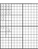
Figure 1: Example of binary matrix(left) and resulting $k^{2}$-tree conceptual representation (right up), and the compact representation (right down), with $k=2$.

2.2 Re-Pair

Re-pair [9] is a grammar-based compression method. Given a sequence of integers $I$ (called terminals), it proceeds as follows: (1) it obtains the most frequent pair of integers $ab$ in $I$, (2) it adds the rule $s\rightarrow ab$ to a dictionary $R$, where $s$ is a new symbol not appearing in $I$ (called a nonterminal), (3) every occurrence of $ab$ in $I$ is replaced by $s$, and (4) it repeats steps 1-3 until every pair in $I$ appears only once (see Figure 2). The resulting sequence after compressing $I$ is called $C$. Every symbol in $C$ represents a phrase (a sequence of 1 or more of the integers in $I$). If the length of the represented phrase is 1, then the phrases consists of an original (terminal) symbol, otherwise it is a new (nonterminal) symbol. Re-Pair can be implemented in linear time, and a phrase can be recursively expanded in optimal time (that is, proportional to its length).

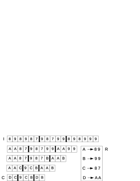
Figure 2: An example of Re-pair compression.

3 Our approach

GraCT represents moving objects that follow free trajectories on the space. We consider the time as discrete, therefore each time instant actually corresponds to a short period of time. We assume that in each time instant, each object informs its position (e.g., international regulations require that ships inform their GPS position at regular intervals). We use a raster model to represent the space, therefore the space is divided into cells of a fixed size, and objects are assumed to fit in one cell. The size of the cells and the period used to sample the time are parameters that can be adapted to the specific domain.

Every $s$ time instants, GraCT uses a data structure based on $k^{2}$-trees to represent the absolute positions of all objects. We call those time instants snapshots. The distance $s$ between snapshots is another parameter of the system. Between two consecutive snapshots the trajectory of each moving object is represented as a log, which is an array of movements, that is, relative positions with respect to the previous time instant.

3.0.1 Snapshots

Each snapshot uses a $k^{2}$-tree where a cell set to 1 indicates that one or more objects are placed in that cell, whereas a 0 means that no object is in that cell. However, we still need to know which objects are in a cell set to 1. Observe that each 1 in the binary matrix corresponds to a bit set to 1 in the bitmap $L$ of the $k^{2}$-tree. We store the list of object identifiers corresponding to each of those bits set to 1 in an array, where the objects identifiers are sorted following the order of appearance in $L$. We call that array perm, since that array is a permutation [8]. In addition, we need a bitmap, called Q, aligned with perm, that informs with a 0 that the object identifier aligned in perm is the last object of a leaf, whereas a 1 signals that more objects exist. Observe in Figure 3, the object identifiers corresponding to the first 1 in $L$ (which is at position 3 of $L$) are stored starting at position 1 of $perm$. In order to know how many objects are in the corresponding cell, we access $Q$ starting at position 1 searching for the first 0, which is at position 2, therefore there are two objects in the inspected cell. By accessing positions 1 and 2 of perm, we obtain the object identifiers 4 and 2. Now, in position 3 of perm starts the object identifiers corresponding to the second 1 in $L$, and so on.

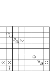
Figure 3: The position of objects in the space (left), and the representing snapshot (right).

With these structures used to represent the absolute positions of all the moving objects at snapshots we can answer two types of queries:

• Find the objects in a given cell: First, using the procedure shown in Section 2.1 to navigate downwards the $k^{2}$-tree, we traverse the tree from the root until reaching the position $n$ in $L$ corresponding to that cell. Next, we count the number of 1s in the array of leaves $L$ until the position $n$; this gives us the number of leaves with objects up to the $n^{th}$ leaf, $x=rank_{1}(L,n)$. Then we calculate the position of the $(x-1)$th 0 in $Q$, which indicates the last bit of the previous leaf (with objects), and we add 1 to get the first position of our leaf, $p=select_{0}(Q,x-1)+1$. Then $p$ is the position in $perm$ of the first object identifier corresponding to the searched position. From $p$, we read all the object identifiers aligned with 1s in $Q$, until we reach a 0, which signals the last object identifier of that leaf.

• Find the position in the space of a given object. First, we need to obtain the position $k$ in perm of the searched object. In order to avoid a sequential search over perm to obtain that position, we add additional structures to compute cells of the inverse permutation of perm [10]. Then, we have to find the leaf in $L$ corresponding to the $k^{th}$ position of $perm$. For this sake, we calculate the number of leaves before the object in position $k$ of perm, that is, we need to count the number of 0s until the position before $k$, $y=rank_{0}(Q,k-1)$. Then we find in $L$ the position of the $(y+1)^{th}$ 1, that is, $select_{1}(L,y+1)$. With that position of $L$, we can traverse the $k^{2}$-tree upwards in order to obtain the position in the space of that cell, and thus the position of the object.

3.0.2 Log of relative movements

The changes that occur between snapshots are tracked using a log file per object. The use of snapshots and logs is not new [16], but in previous works log values are stored according the appearance of “events” (such as objects that appear in or disappear from an area).

The log stores relative movements with respect to the last known position of an object, that is, to its position in the preceding time instant. Objects can change their positions along the two Cartesian axes, so every movement in the log can be described with two integers. Instead, in order to save space, we encode the two values with a unique positive integer. For this sake, we enumerate the cells around the actual position of an object, following a spiral where the origin is the initial object position, as it is shown in Figure 4 (left). Let us suppose that an object moves with respect to the previous known position one cell to the East in the x-axis, and one cell to the North in the y-axis. Instead of encoding the movement as the pair (1,1), we encode it as an 8. In Figure 4 (right) we show the trajectory of an object starting at cell (0,2). Each number indicates a movement between two consecutive time instants. Since most relative movements involve short distances, this technique produces a sequence of usually small numbers.

Figure 4: Encoding object’s movements.

Sometimes real objects stop emitting signals during periods of time. This forces us to add two new possible movements inside a log: relative reappearance and absolute reappearance. We reserve two codewords to signal these events. We use a relative reappearance when an object disappears and reappears between the same snapshots, and an absolute reappearance otherwise. Relative reappearances are followed by the time elapsed from the disappearance and a relative movement from that time instant, whereas absolute reappearances are followed by the number of time instants that elapsed since the disappearance and the absolute values of the $(x,y)$ coordinates of the new position of the object.

4 Compressing the log

The log not only saves much space compared to using $k^{2}$-trees for every instant, but it also offers important opportunities for further compression. A first choice is statistical compression, since as said, most movements are short-distanced and thus our spiral encoding uses mostly small numbers. We exploit this fact using $(s,c)$-Dense Codes (SCDC) [2], a very fast-to-decode statistical compressor that has a low redundancy over the zero-order empirical entropy of the sequence. We will use this approach as fair baseline.

The second approach, which gives the title to this paper, uses grammar compression on the set of all the log files. Our aim is to exploit the fact that there are typical trajectories followed by many objects, which translate into long sequences of identical movements that grammar compression can convert into single nonterminals. This includes, in particular, long straight trajectories in any direction.

4.0.1 ScdcCT: Using SCDC for compressing the logs

The size of the cells and the time elapsed between consecutive time instants must be carefully chosen to represent properly the typical speed of moving objects, so that short movements to contiguous cells are more frequent than movements to distant cells. Instead of sorting the spiral codes by frequency, we will simply assume that smaller numbers are more frequent than larger ones. Since the $(s,c)$-codes depend only on the relative frequency of the symbols, we do not need to store any statistical model. Still, we will use the frequencies to optimize $s$ and $c$ in order to minimize the space usage.

4.0.2 GraCT: Using Re-Pair for compressing the logs

Moving objects spend most of the time either stopped or moving following a specific course and speed. In both cases, the logs will present longs sections with numbers representing the same or contiguous values of the spiral. For example, the moving object in Figure 4 follows a NE trajectory moving one or two cells per time instant. Therefore its log represents the series of relative movements 8,9,8,9,8,7,9,8,7,9; see the array $I$ of Figure 2. Those series of similar movements are very efficiently compressed using a grammar compressor such as Re-Pair. To avoid having to decompress the log before processing it, we enrich the rules of the grammar $R$ with further data apart from the two symbols to be replaced. Specifically, each rule in $R$ will have the following information: $s\rightarrow a,b,\#t,x,y,MBR$, where $s$, $a$ and $b$ are the components of a normal rule of Re-Pair, $\#t$ is the number of instants covered by the rule, $(x,y)$ are the relative coordinates of the final position of the object after the application of the rule, and $MBR$ is the minimum bounding rectangle enclosing the movements of the rule.

For example, the rules of Figure 2 are enriched as follows. The first rule of $R$ is $A\rightarrow 8,~{}9,~{}2,~{}(3,2),~{}(0,0,3,2)$: $8$ and $9$ are the substituted symbols, $2$ indicates that the rule represents a sequence of $2$ movements, $(3,2)$ indicates the position of the object after the application of the rule if we start at $(0,0)$, and the last four values are two points defining a rectangle that encloses all the movements encoded by the rule. The other rules are $B\rightarrow 9,~{}9,~{}2,~{}(4,2),~{}(0,0,4,2)$, $C\rightarrow 8,~{}7,~{}2,~{}(1,2),~{}(0,0,1,2)$, and $D\rightarrow A,~{}A,~{}4,~{}(6,4),~{}(0,0,6,4)$.

Thanks to this additional information, to obtain the position of an object at any time instant between two snapshots, the nonterminal symbols of array $C$ do not need to be decompressed in most cases. Assume we want to know the position of the object at the 5^th time instant, which is when the object in Figure 4 (right) is at position (7,7). The preceding snapshot informs that the absolute position of the object at the beginning of the log is (0,2). Next, we inspect the log (the $C$ array of Figure 2) from the beginning. The first value is a $D$. The enriched rule indicates that such symbol represents 4 time instants, and after it, the object is displaced 6 columns to the East and 4 rows to the North, that is, starting at (0,2), after the application of this rule, the object will be at (6,6). Since our target time instant is later than the final time instant of this rule, we do not have to decompress it, and this is the usual case. The next symbol is $C$, which lasts 2 time instants. This would take us to time instant 6, but this surpasses our target time instant(5). Therefore, in this case, that is, only in the last step of the search, we have to decompress the rule, and process its components: $C\rightarrow 8~{}7$. The 8 is a terminal symbol that lasts 1 time instant, and thus it is enough to reach our target time instant. An 8 moves 1 column to the East and 1 to the North, which applied to the previous position (6,6) takes us to the position (7,7).

The $MBR$ component aids during the computation of time-slice and time-interval queries, as we will see soon.

The additional elements enriching the rules are compressed with an encoder designed for small integers (Directly Addressable Codes, DAC) that support efficient access to any individual value in the sequence [1]. To obtain better compression, the times of all the rules are compressed with one DAC, separately from the 3 pairs of coordinates of all the rules, which are compressed with another.

5 Querying

5.0.1 Obtain the position of an object in a given time instant

This query is solved by accessing the snapshot preceding the queried time instant $t_{q}$, where we retrieve the position of the object at the snapshot time instant. We then apply the movements of the log over this position until we reach $t_{q}$. In the case of SCDC compression, we follow the log decoding each codeword and applying the relative movement to the previous position. In the case of Re-Pair, we follow the process described in the previous section.

5.0.2 Obtain the trajectory of an object between two time instants

First, we obtain the position of the object in the start time instant $t_{s}$, using the same algorithm of the previous query; then we apply the movements of the log until reaching the end time instant $t_{e}$. In this case, when using GraCT, we have to decompress $C$ to recover $I$, since only with $I$ we are capable of describing the trajectory in detail, and thus we cannot take advantage of the enriched nonterminal data. Therefore this query is more time-consuming than the previous one for GraCT, and scdcCT takes over.

5.0.3 Time slice query

Given a time instant $t_{q}$ and a window rectangle $r$ of the space, this query returns the objects that lie within $r$ at time $t_{q}$, and their positions. We can distinguish two cases. First, if $t_{q}$ corresponds to a snapshot, we only need to traverse the $k^{2}$-tree until the leaves, inspecting those nodes that intersect $r$. When we reach the leaves, we know their position and can retrieve from the permutation the objects that are in this area.

The second case occurs when $t_{q}$ is between two snapshots $s_{i}$ and $s_{i+1}$. In this case, we inspect in $s_{i}$ a region $r^{\prime}$, which is an enlargement of the query region $r$. Region $r^{\prime}$ is defined using using the fastest object of the dataset as an upper bound. Thus, $r^{\prime}$ is the rectangle containing all the points from where we can reach the region $r$ at $t_{q}$ if moving at maximum speed along some direction. Then, from $s_{i}$, we only track the objects that are within $r^{\prime}$ in the snapshot, therefore limiting the objects to follow and not wasting time with objects that do not have chances to be in the answer. We follow the movements of those objects from $s_{i}$ using the log, until reaching $t_{q}$. We further prune the tracking as we process the log: a candidate object may follow a direction that takes it away from region $r$, so we recheck the condition after every movement and discard an object as soon as it loses the chance of reaching $r$ at time $t_{q}$.

The tracking of objects is performed with the same algorithm explained for obtaining the position of an object in a given time instant, but in the case of GraCT, when a non terminal in the log corresponds to a rule that brings the object we are following from an instant before to an instant after $t_{q}$, instead of decompressing the nonterminal, we intersect the MBR of the rule with $r$, and disregard the object if the intersection is empty. Otherwise we decompress the nonterminal into two and try again until reaching $t_{q}$ or discarding the object.

Figure 5 shows an example where we want to find the objects that are located in $r$ at $t_{q}$. Assume that the fastest object can move only to an adjacent cell in the period between two consecutive time instants. Let $s_{i}$ be the last snapshot preceding $t_{q}$ and let there be 2 time instants between $s_{i}$ and $t_{q}$. The left part of the figure shows the state of the objects at the time instant corresponding to $s_{i}$, in the middle to $s_{i}+1=t_{q}-1$, and in the right to $t_{q}$, where we show the region $r$. In $r^{\prime}$ (shown on the left grid) we have four elements (1,4,5,8), which are candidates to be in $r$ at $t_{q}$, thus we follow their log movements. In the middle grid, we show the region $r^{\prime\prime}$ where the objects still have chances to be within $r$ at $t_{q}$. Observe that, from the candidate objects in $s_{i}$, object 4 has no further chances to reach $r$, and thus it is not followed anymore. However, object 1 still have chances, and therefore we keep tracking it.

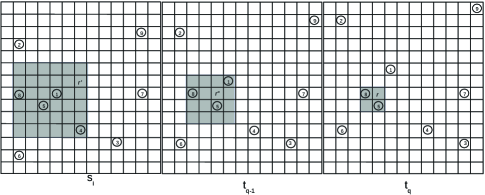
Figure 5: Example of enlarged region $r^{\prime}$ and query region $r$ in a time-slice query.

This query is affected by the time elapsed between $s_{i}$ and $t_{q}$. The farther away $s_{i}$ and $t_{q}$ are, the larger $r^{\prime}$ will be, and thus, we will have more candidate objects that have to be followed through the log movements. In addition, with a large period between $s_{i}$ and $t_{q}$, we have to traverse a longer portion of the log. To alleviate this problem, if $t_{q}$ is closer to $s_{i+1}$ than to $s_{i}$, we can start the search at $s_{i+1}$ and follow backwards the movements of the log. For this backward traversal, we need to add before each snapshot the last known position and its corresponding time instant of the objects that are disappeared at the time instant of the snapshot. This applies to both approaches scdcCT and GraCT. Therefore, the maximum distance will be half of the distance between two snapshots.

5.0.4 Time interval query

In the time-slice query we have to know which objects are in $r$ at the query time instant and their positions, but in the time-interval query, the target is to know which objects were within $r$ at any time instant of the time interval $[t_{s},t_{e}]$, specified in the query. In this case, we use the expanded region $r^{\prime}$ again, which is built as in the time-slice query, but using the time $t_{e}$.

Using SCDC, the objects within $r$ at $t_{s}$ are reported as part of the solution, the other objects with chances at $t_{s}$ are followed until they reach the region $r$, in which case they are added to the answer; or when they move such that they lose the chance to reach $r$ at $t_{e}$, in which case they are not followed anymore.

In GraCT, we process the log without decompressing nonterminal symbols until the final time of a symbol in the log is equal or larger than $t_{s}$. After this moment, for each symbol we read in the log, until the object is selected or the next symbol in the log to read starts after $t_{e}$, we follow the next procedure: For each log symbol we check if the final point is inside $r$. If it is, the object is selected. If not, and the MBR does not intersect $r$, we go on to the next log symbol. If the final point is not in $r$ but the MBR intersects $r$, we must apply the same procedure recursively to the pair of symbols represented by the nonterminal, until the object is selected or we process the whole nonterminal.

6 Experimental Evaluation

GraCT and scdcCT were coded in C++ and the experiments were run on a 1.70GHzx4 Intel Core i5 computer with 8GBytes of RAM and an operating system Linux of 64bits.

6.0.1 Datasets description and compression data

We use a real dataset obtained from the site http://marinecadastre.gov/ais/. The dataset provides the location signals of 3,654 ships during a month. Every position emitted by a ship is discretized into a matrix where the cell size is $50\times 50$ meters. With this data normalization, we obtain a matrix with 100,138,325 cells, 36,775 in the $x$-axis and 2,723 in the $y$-axis. Observe that our structure deals with object positions at regular intervals, but in the dataset ship signals are emitted with distinct frequencies, or they can send erroneous information. Therefore, we preprocessed the signals to obtain regular time instants every minute, thus discretizing the time into 44,642 minutes in one month. With these settings, the original dataset occupies 501 MBs.

	GraCT				scdcCT
Period	120	240	360	720	120	240	360	720
Size (MB)	196.79	193.31	192.24	179.60	312.27	263.46	273.20	282.95
Ratio	39.27%	38.58%	38.36%	35.84%	62.32%	56.47%	54.52%	52.58%
Snapshot (MB)	7.55	3.77	2.51	1.25	7.55	3.77	2.51	1.25
	(3.83%)	(1.95%)	(1.31%)	(0.70%)	(2.42%)	(1.33%)	(0.92%)	(0.48%)
Log (MB)	189.25	189.54	189.73	178.34	304.73	279.18	270.69	262.20
	(96.17%)	(98.05%)	(98.69%)	(99.30%)	(97.58%)	(98.67%)	(99.08%)	(99.52%)

Table 1: Compression ratio.

We built GraCT and scdcCT data structures over that dataset using different snapshot distances, namely every 120, 240, 360, and 720 time instants. The construction time of the complete structure takes around 1 minute. Table 1 shows the results of compression ratio, where we can see that GraCT obtains much better compression ratios than scdcCT. The rows snapshot and log show the size of the snapshot and the log as a percentage of the compressed data structure. We can see that the log is the most space demanding structure. As reference we compress the plain data with p7zip and we obtain a compression ratio of 10,97%, which is better than GraCT, however with this compressed data is impossible to answer any type of query.

6.0.2 Query types and answer times

Table 2 shows the average answer times of 50 random queries of different types: object $t_{q}$ shows searches for the position of an object in a given time instant, trajectory searches for the trajectory followed by an object between two time instants, slice S are time-slice queries that check for small regions ($367\times 272$ cells) and slice L for large regions ($3677\times 2723$ cells), interval S are time-interval queries with a small region and a small time interval ($\frac{1}{10}$ of the snapshot period) and interval L with large regions and a large time interval ($\frac{1}{4}$ of the snapshot period).

	GraCT				scdcCT
Period	120	240	360	720	120	240	360	720
Ratio	39.27%	38.58%	38.36%	35.84%	62.32%	56.47%	54.52%	52.58%
Object $t_{q}$	0.0157	0.0169	0.0210	0.0229	0.0125	0.0169	0.0220	0.0246
Trajectory	0.1582	0.1210	0.1130	0.1153	0.0881	0.0904	0.0900	0.0960
Slice S	1.5386	2.4241	2.9580	5.8788	1.3080	2.6712	4.0430	7.6636
Slice L	1.7835	2.8074	3.6000	6.6430	1.5883	3.8615	5.1130	9.1384
Interval S	2.4435	3.6005	5.0090	9.5635	1.4882	3.8612	5,8610	11.1765
Interval L	2.7505	4.0847	6.1330	12.1832	1.7161	4.9578	9.8680	16.4471

Table 2: Time of different queries (ms).

GraCT is the overall winner in all queries, except in the trajectory query. This is expected, since to recover the trajectory, GraCT has to decode all the symbols in $C$, given that the enriched information in rules does not have the details of the movements inside each rule. In the rest of the queries the enriched information avoids in many cases to decode the rules in $C$, and thus, since the logs in GraCT have far fewer values than in scdcCT, the searches are faster. The exception is when the size of the log between two snapshots is small, as the effect is not noticeable. Notice that in this case the nonterminal symbols in the grammar cannot represent arrays of more than 120 terminals.

7 Conclusions

We have presented a grammar based data structure for representing moving objects. It uses snapshots where the objects are represented in the space using a $k^{2}$-tree and movement logs that are grammar-compressed. The results of this first experimental evaluation are very promising, as compression yields significant reductions in both space and time performance with respect to the baseline.

One reason why our space results are not even better is that the enriched data pose a significant space overhead per nonterminal. We plan to improve our representation by encoding these data in smarter ways. We also plan to compare GraCT with state of the art indexes aimed at both time-slice and time-interval queries, and trajectories.

References

- [1] Brisaboa, N., Ladra, S., Navarro, G.: DACs: Bringing direct access to variable-length codes. Information Processing and Management 49(1), 392–404 (2013)
- [2] Brisaboa, N.R., Fariña, A., Navarro, G., Paramá, J.R.: Lightweight natural language text compression. Information Retrieval 10(1), 1–33 (2007)
- [3] Brisaboa, N.R., Ladra, S., Navarro, G.: Compact representation of web graphs with extended functionality. Information Systems 39(1), 152–174 (2014)
- [4] Chakka, V.P., Everspaugh, A., Patel, J.M.: Indexing large trajectory data sets with SETI. In: Proceedings of the conference on innovative data systems research, CIDR 03 (2003), http://www-db.cs.wisc.edu/cidr/cidr2003/program/p15.pdf
- [5] Gutiérrez, G.A., Navarro, G., Rodríguez, M.A., González, A.F., Orellana, J.: A spatio-temporal access method based on snapshots and events. In: GIS. pp. 115–124. ACM (2005)
- [6] Hadjieleftheriou, M., Kollios, G., Tsotras, V.J., Gunopulos, D.: Efficient indexing of spatiotemporal objects. In: Proceedings of Advances in Database Technology EDBT 2002. pp. 251–268 (2002)
- [7] Jacobson, G.: Space-efficient static trees and graphs. In: IEEE Symposium on Foundations of Computer Science (FOCS). pp. 549–554 (1989)
- [8] Knuth: Efficient representation of perm groups. Combinatorica 11, 33–43 (1991)
- [9] Larsson, N.J., Moffat, A.: Off-line dictionary-based compression. Proceedings of the IEEE 88(11), 1722–1732 (2000)
- [10] Munro, J.I., Raman, R., Raman, V., Rao, S.: Succinct representations of permutations and functions. Theoretical Computer Science 438, 74–88 (2012)
- [11] Nascimento, M.A., Silva, J.R.O.: Towards historical R-trees. In: George, K.M., Lamont, G.B. (eds.) Proceedings of the 1998 ACM symposium on Applied Computing, SAC’98. pp. 235–240. ACM (1998), http://doi.acm.org/10.1145/330560
- [12] Rasetic, S., Sander, J., Elding, J., Nascimento, M.A.: A trajectory splitting model for efficient spatio-temporal indexing. In: Proceedings of the 31st international conference on Very large data bases. pp. 934–945. VLDB Endowment (2005)
- [13] Tao, Y., Papadias, D.: MV3R-tree: A spatio-temporal access method for timestamp and interval queries. In: Apers, P.M.G., Atzeni, P., Ceri, S., Paraboschi, S., Ramamohanarao, K., Snodgrass, R.T. (eds.) Proceedings of 27th International Conference on Very Large Data Bases, VLDB 2001,. pp. 431–440. Morgan Kaufmann (2001)
- [14] Vazirgiannis, M., Theodoridis, Y., Sellis, T.K.: Spatio-temporal composition and indexing for large multimedia applications. ACM Multimedia Systems Journal 6(4), 284–298 (1998)
- [15] Wang, L., Zheng, Y., Xie, X., Ma, W.Y.: A flexible spatio-temporal indexing scheme for large-scale GPS track retrieval. In: Mobile Data Management. pp. 1–8. IEEE (2008)
- [16] Worboys, M.F.: Event-oriented approaches to geographic phenomena. International Journal of Geographical Information Science 19(1), 1–28 (2005)
- [17] Xu, X., Han, J., Lu, W.: RT-tree: An improved R-tree index structure for spatiotemporal databases. In: Proceedings of the 4th International Symposium on Spatial Data Handling. vol. 2, pp. 1040–1049 (1990)