Algorithms for Visibility-Based Monitoring with Robot Teams
Abstract
We study the problem of planning paths for a team of robots for visually monitoring an environment. Our work is motivated by surveillance and persistent monitoring applications. We are given a set of target points in a polygonal environment that must be monitored using robots with cameras. The goal is to compute paths for all robots such that every target is visible from at least one path. In its general form, this problem is NP-hard as it generalizes the Art Gallery Problem and the Watchman Route Problem. We study two versions: (i) a geometric version in street polygons for which we give a polynomial time –approximation algorithm; and (ii) a general version for which we present a practical solution that finds the optimal solution in possibly exponential time. In addition to theoretical proofs, we also present results from simulation studies.
I Introduction
We study the problem of planning paths for a team of robots tasked with visually monitoring complex environments. Visibility-based monitoring problems commonly occur in many applications such as surveillance, infrastructure inspection [1], and environmental monitoring [2]. These problems have received significant interest recently [3, 4, 5], thanks in part, to the technological advances that have made it easy to rapidly deploy teams of robots capable of performing such tasks. For example, Michael et al. [6] demonstrated the feasibility of carrying out persistent monitoring tasks with a team of Unmanned Aerial Vehicles (UAVs) with onboard cameras.
Persistent monitoring problems are typically studied when the points of interest are given as input. The points may have associated weights representing their importance. A common objective is to find the order of visiting the points that minimizes the weighted latency. Alamdari et al. [7] showed that this problem is NP-hard and presented two factor approximation algorithms. In many settings, the path to be followed by the robots is given as input as well, and the speed of the robot must be optimized to minimize the maximum weighted latency. Cassandras et al. [8] presented an optimal control approach to determine the speed profiles for multiple robots when their motion is constrained to a given curve. Yu et al. [9] presented an optimal solution for computing speed profiles for a single robot moving along a closed curve to sense the maximum number of stochastically arriving events on a curve. Pasqualetti et al. [10] presented distributed control laws for coordination between multiple robots patrolling on a metric graph.
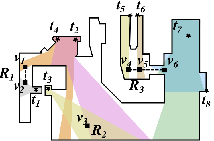
We consider a richer version of the problem where the points to be visited by the robots are not given, and instead must be computed based on visibility-based sensing. We are given a set of target points in a polygonal environment. Each robot carries a camera and can see any target as long as the straight line joining them is not obstructed by the boundary of the environment. Our goal is to compute paths for robots, so as to ensure that each target is seen from at least one point on some path. Figure 1 shows an example scenario for .
Our problem is a generalization of the Art Gallery Problem (AGP) [11] and the Watchman Route Problem (WRP) [12]. The objective in AGP is to find the smallest set of “guard” locations, such that every point in an input polygon is seen from at least one guard. AGP is NP-hard for most types of input polygons [11], and very few approximation algorithms exist even for special cases. The objective in WRP is to find a tour of minimum length for a single robot (i.e., watchman) so as to see every point in an input polygon. There is an optimal algorithm for solving WRP in polygons without any holes [13] and a approximation algorithm for -sided polygons with holes [14]. Carlsson et al [13] introduced –WRP where the goal is to find tours such that each point in the environment is seen from at least one tour. The objective is to minimize the total length of tours. They showed that the problem is NP-hard (in fact, no approximation guarantee is possible).
Using the length of a tour as the cost is reasonable when a robot is capable of obtaining images as it is moving. However, in practice, obtaining high-resolution images while moving may lead to motion blur or cause artifacts to appear due to rolling shutter cameras. This is especially the case when UAVs are to be used. It would be desirable for the robot to stop to obtain a measurement. Instead of finding a continuous path, we would like to find a set of discrete viewpoints on paths. The cost of a path can be modeled as the weighted sum of the length of the path (travel time) and the number of measurements along the path (measurement time). Wang et al. [15] first introduced this objective function for WRP for the case of a single robot and termed it the Generalized WRP (GWRP). They showed that GWRP is NP-hard and presented a approximation for the restricted case when each viewpoint is required to see a complete polygon edge.
We introduce the robot version of GWRP. This problem, in general, is NP-hard since it generalizes the NP-hard problems of GWRP and -WRP. Hence, we consider special instances of the problem and present a number of positive results. In particular, we characterize the conditions under which the problem has an optimal algorithm (Section III) and a present a constant-factor approximation algorithm for a special class of environments (Section IV). In addition to theoretical analysis, we perform simulations to study the effect of the number of robots and targets on the optimal cost.
Finally, we study the case when the measurement time is zero (Section V). We present a practical solution that finds paths for robots. Our solution can be applied for a broad class of environments (e.g., 2.5D, 3D) and can incorporate practical sensing constraints (e.g., limited sensing range and field-of-view). The added generality comes at the expense of running time. Instead of a polynomial time solution, our algorithm may take possibly exponential time. We show how to use existing, sophisticated Traveling Salesperson Problem solvers to produce solutions in reasonable amounts of time (for typical instances).
II Problem Formulation
We study three problems for visibility-based persistent monitoring. The environment is an -sided 2D polygon without holes (in one of the problems we consider a 1.5D terrain111A 1.5D terrain is defined by a continuous (but not necessarily differentiable) function, , which can be interpreted as the height of the terrain at a coordinate . Figure 2(c) gives an example. environment). We are given a set of target points, , within . We have robots each carrying an omnidirectional camera. Let each robot travel with unit speed and let the time to obtain an image be . Let denote both the path and denote the discrete set of viewpoints along this path. Let denote the collection of paths. Let denote the visibility polygon of a point in and denote the union of visibility polygons of all viewpoints on . We relax many of these assumptions for the general case in Section V.
In the first problem, we are given a curve in the polygon along which we must determine the set of viewpoints. The curve can be, for example, the boundary of the environment for border patrolling, or a safe navigation path within the environment. The goal is to find paths along this curve along with viewpoints on the paths, to see every point in . We show that if the set and the curve satisfy a property, termed chain-visibility, then this problem can be solved optimally.

Definition 1.
Let be a set of points and be some curve in a 2D environment. The pair is said to be chain visible if the intersection of the visibility polygon of any point with , i.e., is either empty or a connected chain.
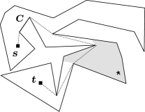
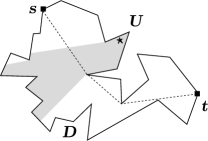
Although restrictive, the chain-visibility property is satisfied by various curves. Figure 2 shows some examples.
Chain-visibility was used by Carlsson and Nilsson [17] to show that there always exists a collapsed watchman path satisfying chain-visibility in street polygons. A street polygon is a polygon without holes with the property that its boundary can be partitioned into two chains, and , and any point in is visible from some point in and vice versa. Figure 2(b) gives an example. We give more examples of chain-visibility in the following proposition.
Proposition 1.
Following pairs of target points of interest, , and curves, , all satisfy the chain-visibility property:
-
•
is any set of points in a street polygon and is a collapsed watchman route.
-
•
is any set of points in a polygon without holes and is the shortest path between any pair of points and in the polygon. In particular, can be a straight line within the polygon.
-
•
is any set of points on a 1.5D terrain and is a fixed altitude path.
Naturally, if the intersection of the visibility region of a point with is empty, we will not be able to compute a viewpoint on to see the point. Hence, we consider only those situations where each point in is visible from some point in while satisfying the chain-visibility property. Formally, the first problem we consider is the following:
Problem 1.
Input: set of points of interest, , and a curve, , such
that is chain-visible
Output: paths each with
viewpoints, , where for all we have .
Objective: .
Contribution: Optimal algorithm
(Section III).
The optimal algorithm for this problem is given in Section III.
In the second problem, is simply the set of all points in the polygon. Our goal is to find paths, restricted to a chain-visible curve, so as to monitor every point in the environment. Here, we focus on the case of street polygons where we know there always exists a curve, namely the collapsed watchman route, which is chain-visible for any subset of points in the polygon [17]. Street polygons have previously been studied in the context of robot navigation in unknown environments [18, 19].
Problem 2.
Input: street polygon, , and a chain-visible curve,
Output: paths, , each with
viewpoints, , where for all we have .
Objective: .
Contribution: –approximation algorithm
(Section IV).
Carlsson and Nilsson [17] presented an optimal algorithm to find the fewest number of viewpoints along to see every point in . One way to compute paths would be to first find this smallest set of viewpoints and then distribute them into paths. Unfortunately, this approach can lead to paths which are arbitrarily longer and consequently arbitrarily worse than optimal paths (Figure 3). Nevertheless, we present a –approximation algorithm for Problem 2.
We consider a general version in the third problem at the expense of discretization. The cost is simply the sum of the distances traveled by the robots. We are given a graph along which the robots can navigate. The robots can stop and take a measurement at the vertices of this graph. We show how to find the optimal solution by reducing this to a TSP instance which can then solved by a numerical solver (e.g., concorde [20]).
Problem 3.
Input: set of points of interest, , and a set of viewpoints, , in a polygon
Output: paths, , where for all we have .
Objective: .
Contribution: optimal solution
(Section V).
The solution is presented in Section V. Our solution extends the single robot solution presented by Obermeyer et al. [21] to the case of multiple robots.
III Optimal Algorithm when Given A Set of Targets and Chain-Visible Curve
In this section, we present an optimal algorithm for solving Problem 1. Here, we are given as input a set of points in an -sided 2D polygon that must be visually monitored. The goal is to find a set of viewpoints along with watchmen paths that visit . The watchmen paths are restricted to an input curve that along with satisfies the chain-visibility property (Definition 1). We show how to compute and find the watchmen paths optimally.
In general, the viewpoints can be anywhere along , i.e., no finite candidate set for is given. We will first establish that there always exists an optimal solution in which is restricted to either endpoint of the intersection of with , where is some point in . Let denote the segment for . For ease of notation, we will assign an ordering of points on the curve . This allows us to define the left and right endpoints for (equivalently, first and last points of along ). We have the following result.
Lemma 1.
There exists an optimal solution for Problem 1 with viewpoints such that for any , if is the left (respectively, right) endpoint of some path , then must be the right (respectively, left) endpoint of some .
The proof is given in the appendix.
This lemma allows us to restrict our attention only to the set of finite (at most ) points on . Furthermore, we need to consider only the right endpoints of all for starting a path, and only the left endpoints for ending a path. We will use dynamic programming to find the optimal starting and ending points of paths. Before we describe the dynamic programming solution, we present a subroutine that is useful in computing the cost of a path when the first and last viewpoint on the path is given.
The subroutine given in Algorithm 1 takes as input a path defined by its first and last viewpoint on . It also takes as input a set of target points that are visible from at least one point along . The output of the subroutine is the optimal set of viewpoints (subject to the condition that first and last point of are included) and the optimal cost of this path. The following lemma proves the correctness of this algorithm.
Lemma 2.
Let be a set of target points and be a chain-visible curve. Let be some path along and be target points visible from . If the first and last viewpoints of are and respectively, then Algorithm 1 computes the optimal set of viewpoints and the optimal cost for .
The proof of correctness in given in the appendix.
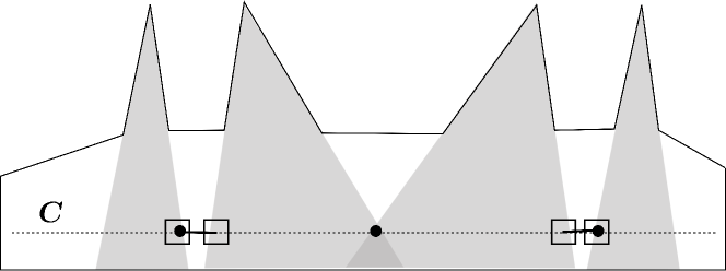
From Lemma 1 we know that all paths in an optimal solution start and end at the right and left endpoints of . Denote the set of all right and left endpoints by and respectively. We build a table of size . The entry gives the maximum cost of the first paths, with the path starting at some and ending at some , and all paths ending before . To correctly fill in the entry , we must ensure that there does not exist any that starts after the path and ends before path (Figure 4). Let be a binary indicator which is if there exists a which is strictly contained between points and , (but does not contain and ). Let Inf be a very large number. We compute as follows.

Let be the first point on . In initializing the entry we must ensure that there is no target such that ends before . Thus, for all to and to we initialize,
To fill the rest of the entries, we first find points and given ,
| (1) |
The term ensures that there is no that starts after but ends before . Furthermore, since the path ends at , we know all that start before will be covered. This only leaves two types of points to consider: (i) starts after but does not end before , and (ii) starts after . While filing in we first compute according to Equation 1. Then, we verify if there exists any point belonging to either of the two types listed above. If not, then all points in have already been covered by the first paths. Hence, we set . If there is exists a point belonging either of the two types listed, then
Additionally, if we must check if there is any point which has not been covered. Let be the rightmost point of the curve . If , we set to .
To recover the final solution, we have to find the entry with the least cost. Using additional book-keeping pointers, we can recover the optimal solution by standard dynamic programming backtracking. The following theorem summarizes our main result for this section.
Theorem 1.
There exists a polynomial time algorithm that finds the optimal solution for Problem 1.
The property in Lemma 1 allowed us search over a finite set of points for computing the endpoints of the paths. This comes from the finiteness of the set . Now, consider the case when all points in a polygon are to be monitored by the robots. We may have possibly infinite candidate endpoints for the optimal paths along . Nevertheless, in the next section we will show how to compute an approximation for the optimal paths in finite time.
III-A Simulations
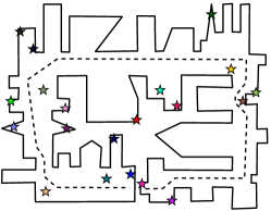
The algorithm was implemented in MATLAB using the VisiLibity [22] library for floating-point visibility computations. The polygonal environment shown in Figure 5(a) was used to generate all the simulation instances.
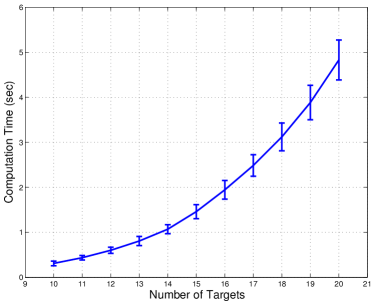
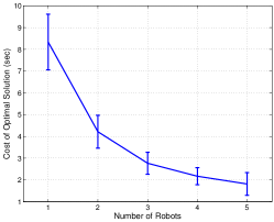
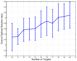
The simulation results are presented in Figure 5. The plots show mean and standard deviation of the costs for 50 trials. The positions of the targets are randomly generated for each trial. All target locations are generated such that they satisfy the chain-visibility property with respect to the dashed path shown in Figure 5(a). The measurement time was set to s for all trials.
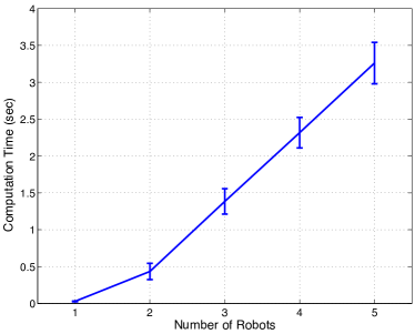
Figure 5(b) shows the effect of varying the number of robots on the optimal cost (makespan). 15 target locations are randomly generated for each trial. Figure 5(c) shows the effect of varying the number of targets. The number of robots were fixed to 3. Figure 6 shows the computation time required for running the dynamic programming, as a function of the number of robots and the targets.
IV –Approximation For Street Polygons
In this section, we present a –approximation algorithm for Problem 2. The input to the problem is a street polygon (see Figure 2(b) for an example) and a curve that satisfies the chain-visibility property for all points in . Carlsson and Nilsson [17] showed that there always exists such a curve for street polygons, known as the collapsed watchman route. They also presented an algorithm to compute the smallest set of discrete viewpoints along such a curve to see every point in . As shown in Figure 3 constructing paths directly from the optimal set of discrete viewpoints can lead to arbitrarily worse solutions for Problem 2. Nevertheless, in this section, we will present an algorithm that yields a –approximation starting with the smallest set of discrete viewpoints.
Let and be the first and last points of the input curve . Let and by any points on ( to the left of ). Let denote the set of all points on between and . We use the following definition of a limit point of a point adapted from [17].
Definition 2.
The limit point of a point on , denoted by , is defined as the first point on to the right of such that is the right endpoint of for any .222The closure of a set of points is the union of the set of points with its boundary.
In other words, is the right endpoint of a closest to and to its right, such that is not visible from any point to the left of , including . Figure 7 shows an example.
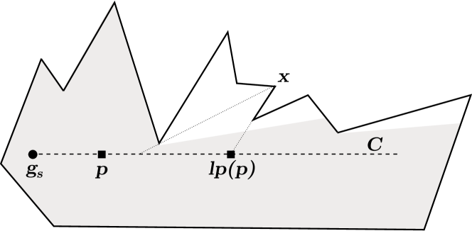
In the previous section, we implicitly used the concept of a limit point in Line 1 of Algorithm 1. The limit point of any point given a curve can be computed efficiently in polynomial time [17], which we will use in our algorithm. For the first limit point, we have the following result.
Lemma 3 ([17]).
If is the first point on to the right such that is the right endpoint of for any , then
Carlsson and Nilsson [17] also presented an algorithm to compute the first viewpoint satisfying the above condition.
It is easy to see that any solution where the first path starts before can be converted to another valid solution of equal or less cost where the first path starts at . The subroutine given in Algorithm 2 starts with to compute paths. Let be the cost of the optimal solution for some instance of Problem 2. The subroutine takes as input a guess for , say . We first compute the smallest set of viewpoints sufficient to see every point in the environment using [17]. The rest of the algorithm constructs paths such that the cost of each path is at most .
Lemma 6 shows if the set of paths computed by the algorithm does not see every point in , then our guess for is too small. Thus, we can start with a small initial guess for , say , and use binary search to determine the optimal value . Since all tours computed cost less than , we obtain a –approximation when our guess .
We first prove that the discrete set of viewpoints computed by Algorithm 2 are correct.
Lemma 4.
Let be the last point on the last path and be the set of all viewpoints over all paths given by Algorithm 2. If a point is visible from , then is also visible from the discrete set of viewpoints .
Proof.
Suppose there is a point visible from which is not visible from any point in . Let and be the left and right endpoints of . must lie to the left of since is visible from . Similarly, must lie to the left of otherwise since , will be covered by . From Lemma 3 and the fact that , must lie to the right of . Thus we have . We omit the rest of the proof since it is similar to that of Lemma 2.
Lemma 5.
Let be the set of paths computed using Algorithm 2 and be the last endpoint of the rightmost path. Let be any set of paths with the last endpoint of the rightmost path, such that all points visible from are covered by . If the cost of is at most , then cannot be to the right of .
Proof.
From Lemma 3 and the definition of limit point, we can say that the first path in starts from . We will prove the lemma by induction on the index of the path. Specifically, we will show that the right endpoint of the path in , say , cannot be to the left of the right endpoint of the path in , say . For ease of notation, we will refer to the left endpoint of the path by and correspondingly .
Base case. We have two possibilities: (i) is away from , (ii) contains at least viewpoints from . For (i), since the cost of is at most , its length cannot be greater than . Hence, cannot be to the right of . For (ii), suppose is to the right of . Then must contain at least viewpoints from the optimality of . Thus, the cost of is greater than which is a contradiction. The base of the induction holds.
Inductive step. Suppose that is to the left or coincident with . We claim that must be to the left or coincident with . Suppose not. By construction, . Let be a point such that is the right endpoint of and is not visible from . Such an always exists according to the definition of a limit point. Hence, lies completely between and implying is not covered by , which is a contradiction. Hence, is to the left or coincident with . Now, using an argument similar to the base case, we can show that cannot be to the right of proving the induction.
Hence, for all , cannot be to the right of proving the lemma.
Lemma 6.
If Algorithm 2 returns Failure then .
Proof.
Suppose . Let be the optimal set of paths. Let and be the rightmost points on and respectively. From Lemma 5, we know cannot be to the right of .
We now bound the cost of the solution produced by our subroutine.
Lemma 7.
The maximum cost of any path produced by Algorithm 2 is at most .
Proof.
By construction, the length of any path is at most . The number of measurements are at most . Hence, the cost of any path is at most .
Combining all the above lemmas, we can state our main result for this section.
Theorem 2.
There exists a –approximation for Problem 2.
The minimum number of discrete viewpoints can be significantly larger than the number of vertices of the polygon. can be computed in time polynomial in the input size (i.e., the number of sides in the input polygon) and the output size (i.e., ). Consequently, the running time for each invocation of the subroutine in Algorithm 2 is also polynomial in the input and output size. The optimal value can be computed in invocations of the subroutine via binary search. We can reduce the overall running time by terminating the binary search early, at the expense of the approximation factor.
V General Solution
In this section, we address the general case for the multi-robot watchmen route problem. We remove the restriction of street polygons and requiring a chain-visible curve as input. However, the added generality comes at the expense of some relaxations. We assume that a finite set of candidate measurement locations, , is given as input. The goal is to find tours for each robot visiting a subset of such that they collectively see all the targets. Note that there is no further assumption (e.g., chain-visibility) on . Consequently, can be computed by simply discretizing the environment either uniformly or using the strategy in Deshpande et al. [23]. Instead of minimizing the maximum times of the tour, we resort to minimizing the sum of the length of all tours (i.e., ).
Our contribution is to show how to solve this general version of the multi-robot watchman route problem by reducing it to a TSP instance. The resulting TSP instance is not necessarily metric, and consequently existing polynomial time approximation algorithms cannot be directly applied. Instead, we directly find the optimal TSP solution leveraging sophisticated TSP solvers (e.g., concorde [20]). This is motivated by recent work by Mathew et al. [24] who used a similar approach for solving a multi-robot rendezvous problem. We demonstrate that this algorithm finds the optimal solution faster than directly solving the original problem using an Integer Linear Programming solver.
In the following we describe our reduction and prove its correctness. We also present empirical results from simulations for a 2D case. However, the following algorithm also works for 3D problems and can incorporate additional sensing range and motion constraints.
V-A Reduction to TSP
Let denote the environment in which the targets points are located. We are given a set of candidate viewpoints within . We denote the viewpoint by where . For each target , we create cluster of viewpoints, . Without loss of generality, we assume that is such that each target is seen from at least one viewpoint (i.e., for all ). One way of generating a valid set is by sampling or discretizing the visibility polygons for all . For the special case, when is the set of all points in a 2D polygon, we can generate by imposing a grid inside using the strategy from [23].
If a robot visits any viewpoint in cluster , then it ensures that target is seen by the corresponding robot. Therefore, the goal is to find a set of tours, one per robot, such that at least one viewpoint in each is visited. Note that the clusters need not be disjoint. This problem is equivalent to the multi-robot Generalized Traveling Salesman Problem (GTSP) [25].
The input to GTSP is a set of clusters, each containing one or more nodes from a connected graph. The goal in single robot GTSP is to find the minimum length tour that visits at least one node in each cluster.333There are versions of GTSP with additional restrictions of visiting exactly one node in each cluster or visiting each cluster exactly once. We consider the less restrictive version where the robot is allowed to visit a cluster multiple times while still ensuring a specific node is visited no more than once. GTSP is NP-hard [25] since it generalizes TSP.
Noon and Bean [26] and Lien and Ma [25] presented two polynomial time reductions of GTSP into a TSP instance such that the optimal TSP tour yields the optimal GTSP solution. The resulting TSP instance is not necessarily metric and consequently the standard approximation algorithms (e.g., [27]) cannot be applied. We can find the optimal solution of the TSP instance directly using potentially exponential time algorithms. A number of sophisticated implementations have been developed for solving large TSP instances to optimality [20]. In particular, we use the concorde solver which yields the best-known solutions to large TSP instances [28]. In Section V-B, we compare this approach with a generic Integer Linear Programming solver.
The reductions from GTSP to TSP proposed by Noon and Bean [26] and Lien and Ma [25] are for finding a single robot GTSP tour. In our case, we are interested in finding tours – one for each of the robots. Mathew et al. [24] presented a multi-robot extension for the Noon-Bean transformation. This transformation is applicable for the case when the clusters in the GTSP instance are disjoint (i.e., , for all ). With slight modification, we can apply the transformation to the case of possibly overlapping clusters as given below.
We assume that the path for the robot must start at a specific vertex, , and end at a specific vertex . We model three scenarios:
-
1.
SameDepot: All robots start and finish their tours at the same location. That is, for all and .
-
2.
SameFinishDepot: All robots finish their tours at the same location but may have unique starting locations. That is, for all and .
-
3.
InterchangeableDepots: There are fixed depots and initially there is one robot at each depot. The robots can end their paths at any of the depots with the restriction that each depot must have one robot at the end.
For all the scenarios, the algorithm given below finds tours such that the sum of the lengths of all tours is minimized and each target is seen.
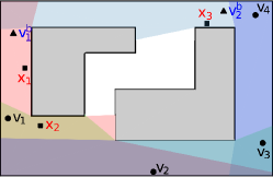
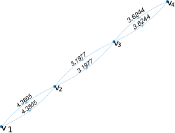
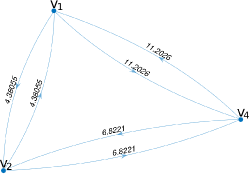
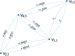
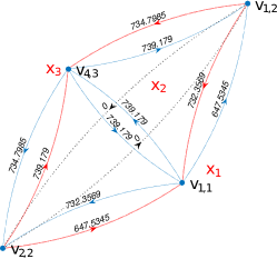
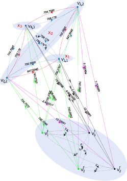
The reduction consists of five main steps. First, represent the given instance as a graph. Second, form a metric completion of the graph and remove viewpoints that cannot see any target. Third, convert the overlapping clusters to non-overlapping ones. Fourth, use a modified Noon-Bean reduction [26] to convert the GTSP instance into a TSP instance. Fifth, add start and finish depots as nodes in the graph. The detailed description of each step is given below.
- 1.
-
2.
(Figures 8(b) to 8(c)) Complete the graph in Step-1 to give ). Cost of an edge in is equal to the cost of shortest path between and in . Then, remove isolated nodes that are not present in any cluster in . This in turn removes edges }. Above operations give us =() where and . 444The completion may result in some nodes to be visited multiple times in the final tour.
-
3.
Carry out the first step in Noon-Bean transformation [26], the I-N transformation, as follows: is converted to a graph that has non-intersecting set of clusters. We go through following steps:
-
•
Create set of nodes .
-
•
Create set of clusters = where .
-
•
For all nodes of the form where , create an ‘intranode-intercluster’ edge () and assign a zero cost to this edge.
- •
-
•
Choose greater than the cost of any tour in that visits all targets . Add this penalty to all edges in except zero cost edges.555We use the cost of an arbitrary tour in the original GTSP for this step instead of using sum of the cost of all the edges as used in P2 of Noon-Bean Method [26]. This is used to prevent numerical issues with large penalties in concorde. The exact expression for will be defined in Step 5.
-
•
-
4.
Complete the Noon-Bean reduction by adding intracluster edges, tail-shifting, and imposing another penalty. Convert to a new graph as follows:
-
•
Copy the vertices, edges and clusters: , , and . Create edges to connect all nodes in cluster by an intracluster cycle in any order. That is, . Here represents an edge (). To mark these edges we assign a cost of to them. Add these edges to .
-
•
For all intercluster edges where , we move the tail of all edges to the previous node in the intracluster cycle defined above. That is, changes to .
-
•
We choose a cost to be greater than cost of any tour in the environment that visits all targets with a penalty added to each of the edges in the tour. Add this penalty to all edges in except those marked with costs. Replace the cost of all the edges with cost to a cost of zero.
-
•
-
5.
Add robot depots to the graph. Create a new graph . For all the depots, add and to . For the InterchangeableDepots we create two copies of each depot. For SameDepot we create copies of the depot, and for SameFinishDepot we create copies of the finish depot. Create zero cost edges between all pairs of depot nodes. We get the final directed TSP graph . Here and . We also add the following edges to :
-
•
Create depot outgoing edges . Assign a cost to all edges equal to the cost of the shortest path connecting to in restricted to . Also, add a penalty to these edges. Add to .
-
•
Create tail shifted depot incoming edges . Also, add the cost to as above but without penalty. Then we move tail of all the edges to the previous node in the intracluster cycle defined in Step 4 above. That is, changes to . Add to .
-
•
Define =2(cost of MST in )+cost in . Define =((edges in MST in ))+().
-
•
-
6.
This gives us a directed TSP input instance. This can be converted to an undirected TSP using transformation used by Karp [29].
The correctness of the algorithm follows from the correctness of the original Noon-Bean reduction [26]. The major change to the reduction is the addition of the complete graph between the depot vertices, . The only incoming edges to the start depots, , are from the finish depot vertices, . Similarly, the only outgoing edges from the finish depot vertices are to the start depot vertices. Consequently, whenever the optimal TSP tour visits a finish depot vertex it must take a zero cost edge to a start depot vertex, from which it may either to a node in or to another finish depot vertex. Therefore, the TSP tour visits an alternating sequence of start and finish depot vertices with possibly non-zero viewpoints (i.e., vertices) in between. We can therefore partition the TSP tour into subtours from start depot to finish depots. This gives us paths for the robots. One or more of these subtours may be empty, in which case the optimal solution uses fewer than robots. This can happen since the algorithm minimizes the sum of the path lengths, and not the maximum path length of robots.
V-B Computational Studies
We implemented the algorithm described in the previous subsection. Our implementation is available online at https://github.com/raaslab/watchman_route and uses the Noon-Bean implementation from Mathew et al. [24] and VisiLibity library [22]. Figure 8 shows a 2D instance solved using this algorithm.
The penalties added to the edges can cause their cost to become large enough to run into numerical overflow issues. In our experiments, we encountered instances where the penalty resulted in the edge costs becoming large than what can be represented with the data structure used by concorde. In such a case, we can use the reduction given by Lien and Ma [25] which does not require the addition of any penalty. However, their reduction triples the number of nodes in the TSP as compared to the Noon-Bean transformation. This results in larger instances and slower running times. Our single robot implementation based on the Lien-Ma transformation is also available online.
An instance with 15 targets and 30 candidate viewpoints for one robot took 41s secs to solve using concorde, where as the same instance took 536s to solve directly using the Integer Linear Programming solver in MATLAB. We use an iterative implementation [30] to find the tour in MATLAB using the ILP function since specifying the full problem directly becomes too large to hold in memory.
| Reduction | Solver | Problem Size | Time (secs) |
|---|---|---|---|
| Lien-Ma | concorde (DFS) | , | 159.97 |
| Lien-Ma | concorde (BFS) | , | 225 |
| — | MATLAB ILP | , | 40 |
| Noon-Bean | concorde (BFS) | , | 2.7 |
Table I gives the times required to solve some representative problems using the Lien-Ma and Noon-Bean reductions with concorde and MATLAB. As expected, the Noon-Bean reduction along with the concorde solver is fastest among all options. The Lien-Ma reduction for an instance with 15 targets and 30 candidate viewpoints could not be solved in 12 hours using concorde. An instance with and could not be solved using MATLAB’s ILP function in more than 16 hrs of computation. The same instance took 2411 secs with concorde and Noon-Bean reduction. An instance with , , and three robots was solved in 1599 secs with concorde and Noon-Bean.
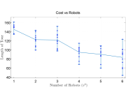
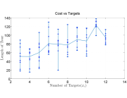
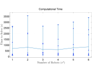
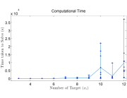
Figure 9(a) shows the effect of varying the number of robots on the optimal cost (sum of path lengths). 10 target locations are randomly generated for each trial in the environment shown in Figure 10. Figure 9(b) shows the effect of varying the number of targets. The number of robots were fixed to 3. Figures 9(c)–(d) show the computation time required for finding the solution using the Noon-Bean reduction with concorde (BFS) solver, as a function of the number of robots and the targets.
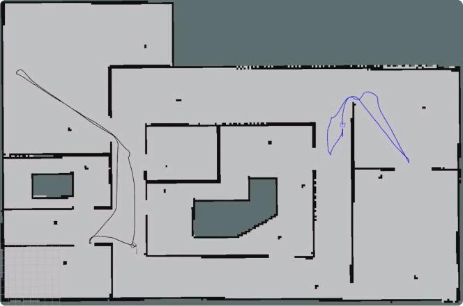
The resulting algorithm was also tested in the Gazebo simulation environment (Figure 10) using two Pioneer 3DX robots fitted with a limited field-of-view angle camera. The robots emulate an omni-directional camera by rotating in place whenever they reach a new vertex. Table II shows the comparison between the lengths of the tours on the input graph and the actual distance traveled by the robots in the Gazebo simulation environment. The actual distances are shorter since the robot is not restricted to move on the input graph in the polygonal environment.
| Length of Tour Computed | Actual Distance Traveled | |
|---|---|---|
| Robot 1 | 78.06 | 71.74 |
| Robot 2 | 50.04 | 43.63 |
VI Discussion and Conclusion
Our approach in this paper was to formulate a geometric version of the persistent monitoring problem with a more abstract but generalizable specification. Even with this formulation, the problem turns out to be challenging.
The analysis presented is based on the key property of chain-visibility which is satisfied by limited classes of environments. In particular, for Problem 2 we require the environment to be a street polygon. One approach of extending our algorithm for general environments would be to first decompose the environment into street polygons, and then apply our algorithm separately in each component. While algorithms for decomposition into street polygons are not known, there is an optimal algorithm for decomposing a polygon without holes into the fewest number of monotone subpolygons [31]. The class of monotone polygons are included in the class of street polygons, and thus can be used as valid inputs to our algorithm. Alternatively, human operators may be able to provide this decomposition. However, in both cases, the approximation guarantee will in general not hold.
The main open problem from a theoretical standpoint is whether there are polygons for which we can compute optimal solutions or constant-factor approximations for watchmen routes without requiring a candidate input curve. One possible approach would be to determine settings in which we can first compute a discrete set of viewpoints and then find paths to visit them. There are existing algorithms for finding paths of minimum maximum length to visit a set of points (see e.g., [32]). The key property would be to show that a tour restricted to the discrete set of viewpoints thus computed is at most a constant factor away from an optimal tour. The approximation algorithm presented in Section IV follows this principle. Investigating similar results for richer environments is part of our ongoing work.
The algorithm in Section V finds the optimal solution by reducing it to GTSP. However, this is valid when the cost function is the sum of the travel times for all the robots. Extending this approach to account for measurement time, and minimizing the makespan remains an open problem.
References
- [1] T. Ozaslan, S. Shen, Y. Mulgaonkar, N. Michael, and V. Kumar, “Inspection of penstocks and featureless tunnel-like environments using micro uavs,” in International Conference on Field and Service Robotics, 2013.
- [2] R. N. Smith, M. Schwager, S. L. Smith, B. H. Jones, D. Rus, and G. S. Sukhatme, “Persistent ocean monitoring with underwater gliders: Adapting sampling resolution,” Journal of Field Robotics, vol. 28, no. 5, pp. 714–741, 2011.
- [3] S. L. Smith, M. Schwager, and D. Rus, “Persistent robotic tasks: Monitoring and sweeping in changing environments,” Robotics, IEEE Transactions on, vol. 28, no. 2, pp. 410–426, 2012.
- [4] J. Yu, M. Schwager, and D. Rus, “Correlated orienteering problem and its application to informative path planning for persistent monitoring tasks,” in IEEE/RSJ International Conference on Intelligent Robots and Systems, 2014.
- [5] X. Lan and M. Schwager, “Planning periodic persistent monitoring trajectories for sensing robots in gaussian random fields,” in Robotics and Automation (ICRA), 2013 IEEE International Conference on. IEEE, 2013, pp. 2415–2420.
- [6] N. Michael, E. Stump, and K. Mohta, “Persistent surveillance with a team of mavs,” in Intelligent Robots and Systems (IROS), 2011 IEEE/RSJ International Conference on. IEEE, 2011, pp. 2708–2714.
- [7] S. Alamdari, E. Fata, and S. L. Smith, “Persistent monitoring in discrete environments: Minimizing the maximum weighted latency between observations,” The International Journal of Robotics Research, vol. 33, no. 1, pp. 138–154, 2014.
- [8] C. G. Cassandras, X. Lin, and X. Ding, “An optimal control approach to the multi-agent persistent monitoring problem,” Automatic Control, IEEE Transactions on, vol. 58, no. 4, pp. 947–961, 2013.
- [9] J. Yu, S. Karaman, and D. Rus, “Persistent monitoring of events with stochastic arrivals at multiple stations,” in IEEE International Conference on Robotics and Automation (ICRA), 2014.
- [10] F. Pasqualetti, J. W. Durham, and F. Bullo, “Cooperative patrolling via weighted tours: Performance analysis and distributed algorithms,” Robotics, IEEE Transactions on, vol. 28, no. 5, pp. 1181–1188, 2012.
- [11] J. O’rourke, Art gallery theorems and algorithms. Oxford University Press Oxford, 1987.
- [12] W.-p. Chin and S. Ntafos, “Optimum watchman routes,” Information Processing Letters, vol. 28, no. 1, pp. 39–44, 1988.
- [13] S. Carlsson, H. Jonsson, and B. J. Nilsson, “Finding the shortest watchman route in a simple polygon,” Discrete & Computational Geometry, vol. 22, no. 3, pp. 377–402, 1999.
- [14] J. S. Mitchell, “Approximating watchman routes,” in Proceedings of the Twenty-Fourth Annual ACM-SIAM Symposium on Discrete Algorithms. SIAM, 2013, pp. 844–855.
- [15] P. Wang, R. Krishnamurti, and K. Gupta, “Generalized watchman route problem with discrete view cost,” International Journal of Computational Geometry & Applications, vol. 20, no. 02, pp. 119–146, 2010.
- [16] P. Tokekar and V. Kumar, “Visibility-based persistent monitoring with robot teams,” in Proceedings of IEEE/RSJ International Conference on Intelligent Robots and Systems (IROS). IEEE, September 2015, pp. 3387–3394.
- [17] S. Carlsson and B. J. Nilsson, “Computing vision points in polygons,” Algorithmica, vol. 24, no. 1, pp. 50–75, 1999.
- [18] C. Icking, R. Klein, E. Langetepe, S. Schuierer, and I. Semrau, “An optimal competitive strategy for walking in streets,” SIAM Journal on Computing, vol. 33, no. 2, pp. 462–486, 2004.
- [19] C. Icking, T. Kamphans, R. Klein, and E. Langetepe, “On the competitive complexity of navigation tasks,” in Sensor Based Intelligent Robots. Springer, 2002, pp. 245–258.
- [20] D. Applegate, R. Bixby, V. Chvatal, and W. Cook, “Concorde tsp solver,” URL http://www. tsp. gatech. edu/concorde, 2006.
- [21] K. J. Obermeyer, P. Oberlin, and S. Darbha, “Sampling-based path planning for a visual reconnaissance unmanned air vehicle,” Journal of Guidance, Control, and Dynamics, vol. 35, no. 2, pp. 619–631, 2012.
- [22] K. J. Obermeyer and Contributors, “The VisiLibity library,” http://www.VisiLibity.org, 2008, r-1.
- [23] A. Deshpande, T. Kim, E. Demaine, and S. Sarma, “A pseudopolynomial time o (log n)-approximation algorithm for art gallery problems,” Algorithms and Data Structures, pp. 163–174, 2007.
- [24] N. Mathew, S. L. Smith, and S. L. Waslander, “Multirobot rendezvous planning for recharging in persistent tasks,” IEEE Transactions on Robotics, vol. 31, no. 1, pp. 128–142, 2015.
- [25] Y. N. Lien, E. Ma, and B. W. S. Wah, “Transformation of the generalized traveling-salesman problem into the standard traveling-salesman problem,” Information Sciences, vol. 74, no. 1-2, pp. 177–189, 1993.
- [26] C. E. Noon and J. C. Bean, “An efficient transformation of the generalized traveling salesman problem,” INFOR, vol. 31, no. 1, p. 39, 1993.
- [27] S. Arora, “Polynomial time approximation schemes for euclidean tsp and other geometric problems,” in Foundations of Computer Science, 1996. Proceedings., 37th Annual Symposium on. IEEE, 1996, pp. 2–11.
- [28] D. L. Applegate, R. E. Bixby, V. Chvatal, and W. J. Cook, The traveling salesman problem: a computational study. Princeton university press, 2011.
- [29] R. M. Karp, “Reducibility among combinatorial problems,” in Complexity of computer computations. Springer, 1972, pp. 85–103.
- [30] “Iterative integer linear programming method for travelling salesman problem,” https://www.mathworks.com/help/optim/ug/travelling-salesman-problem.html, accessed: 2016-11-04.
- [31] J. M. Keil, “Decomposing a polygon into simpler components,” SIAM Journal on Computing, vol. 14, no. 4, pp. 799–817, 1985.
- [32] E. M. Arkin, R. Hassin, and A. Levin, “Approximations for minimum and min-max vehicle routing problems,” Journal of Algorithms, vol. 59, no. 1, pp. 1–18, 2006.
Proof of Lemma 1
Proof.
Consider the case when is the left endpoint of a path in an optimal solution. We will prove by contradiction. If is not also the right endpoint of some , then find the first right endpoint, say , of some that is to the right of along . All points in visible from are also visible from . Thus, we can let be the new left endpoint of to give a valid solution of lesser length, i.e. lesser cost, which is a contradiction. The case for the right endpoint is symmetrical.
Proof of Lemma 2
Proof.
We first verify that all targets in will be covered by the algorithm (and thus the algorithm terminates). Suppose not. Let be a target that is not covered. By definition of , intersects with . Let and be the left and right endpoints of . If is to the left of , then is visible from and will be marked covered. If is to the right of , then is visible from and will be marked covered. Hence, and lie between and .
Consider the closest viewpoint in lying to the left of , say (we know at least one such viewpoint exists, namely ). Let be the first viewpoint in to the right of (we know at least one such viewpoint exists, namely ). Now cannot be to the left of , else is not the closest viewpoint to the left of . Similarly, cannot be to the right of since will not satisfy the condition in Line 1 in Algorithm 1. This leaves the case where is between and , in which case is visible from a viewpoint in .
Next, we verify that the optimal set of viewpoints and cost is correctly computed. The length of is fixed since and are given as input. Let be the subset of such that any is not visible from either or . It remains to show that is the least number of measurements required to cover . Denote the viewpoints in by . Along with and , this defines partitions: .
For contradiction, suppose there is a with viewpoints that cover . Then, there must exist at least one partition that does not contain any . From Line 1, this implies that there is some point whose interval lies completely between two consecutive viewpoints in . Thus, does not cover all elements in which is a contradiction.