Understanding and Mapping Natural Beauty
Abstract
While natural beauty is often considered a subjective property of images, in this paper, we take an objective approach and provide methods for quantifying and predicting the scenicness of an image. Using a dataset containing hundreds of thousands of outdoor images captured throughout Great Britain with crowdsourced ratings of natural beauty, we propose an approach to predict scenicness which explicitly accounts for the variance of human ratings. We demonstrate that quantitative measures of scenicness can benefit semantic image understanding, content-aware image processing, and a novel application of cross-view mapping, where the sparsity of ground-level images can be addressed by incorporating unlabeled overhead images in the training and prediction steps. For each application, our methods for scenicness prediction result in quantitative and qualitative improvements over baseline approaches.
1 Introduction
Recent advances in learning with large-scale image collections have led to methods that go beyond identifying objects and their interactions toward quantifying seemingly subjective high-level properties of the scene. For example, Isola et al. [6] explore image memorability, finding that memorability is a stable property of images that can be predicted based on the image attributes and features. Other similar high-level image properties include photographic style [28], virality [4], specificity [7], and humor [3]. Quantifying such properties facilitates new applications in image understanding.
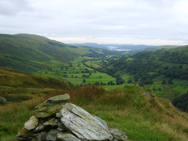
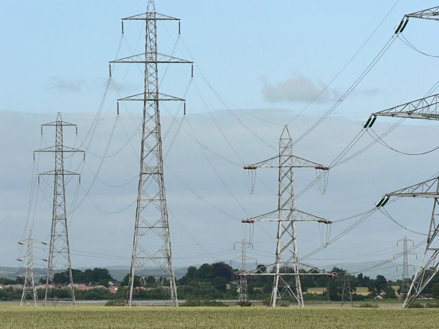
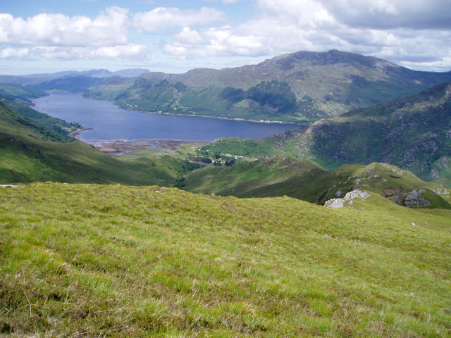
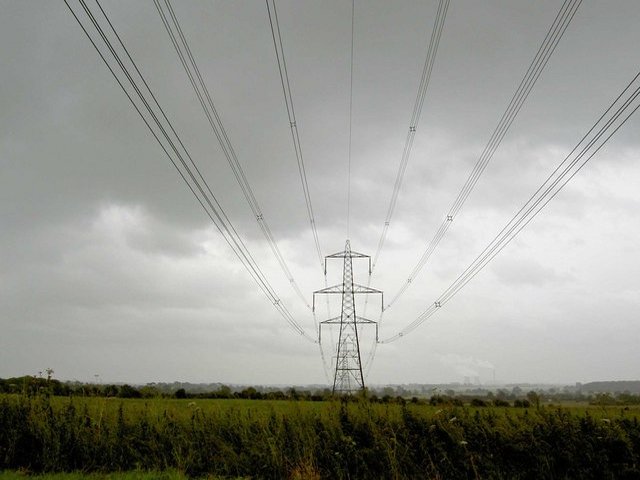
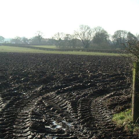
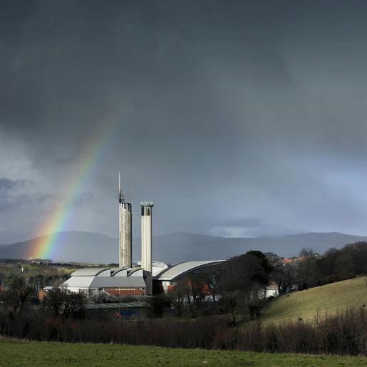
In this paper we consider “scenicness”, or the natural beauty of outdoor scenes. Despite the popularity of the saying “beauty lies in the eye of the beholder,” research shows that beauty is not purely subjective [12]. For example, consider the images in Figure 1; mountainous landscapes captured from an elevated position are consistently rated as more beautiful by humans than images of power transmission towers.
Understanding the perception of landscapes has been an active research area (see [41] for a comprehensive review) with real-world importance. For example, McGranahan [19] derives a natural amenities index and shows that rural population change is strongly related to the attractiveness of a place to live, as well as an area’s popularity for retirement or recreation. Seresinhe et al. [26] show that inhabitants of more beautiful environments report better overall health. Runge et al. [24] characterize locations by their visual attributes and describe a system for scenic route planning. Lu et al. [16] recover cues from millions of geotagged photos to suggest customized travel routes.
Recently, a number of algorithms have been developed to automatically interpret high-level properties of images. Laffont et al. [11] introduce a set of transient scene attributes and train regressors for estimating them in novel images. Lorenzo et al. [21] use a convolutional neural network to estimate urban perception from a single image. Deza and Parikh [4] study the phenomenon of image virality. Similarly, a significant amount of work has sought to understand the relationship between images and their aesthetics [10, 18, 37]. Karayev et al. [9] recognize photographic style. Su et al. [28] propose a method for scenic photo quality assessment using hand-engineered features. Developed independently from our work, Seresinhe et al. [25, 27] explore models for quantifying scenicness. Lu et al. [15] apply deep learning to rate images as high or low aesthetic quality.
In this paper, we start with a large-scale dataset containing hundreds of thousands of images, individually rated by humans, to quantify and predict image scenicness. Our main contributions are:
-
•
an analysis of outdoor images to identify semantic concepts correlated with scenicness;
-
•
a method for estimating the scenicness of an image which accounts for variance in the ratings and human perception of scenicness;
-
•
a new dataset of ground-level and overhead images with crowdsourced scenicness scores; and
-
•
a novel cross-view mapping approach, which incorporates both ground-level and overhead imagery to address the spatial sparsity of ground-level images, to provide country-scale predictions of scenicness.
2 Exploring Image Scenicness
Our work builds on a publicly-available crowd-sourced database collected as part of an online game, ScenicOrNot,111ScenicOrNot (http://scenicornot.datasciencelab.co.uk/) is built on top of Geograph (http://www.geograph.org.uk/), an online community and photo-sharing website. which contains images captured throughout Great Britain. As part of the game, users are presented a series of images from around the island of Great Britain and invited to rate them according to their scenicness, or natural beauty, on a scale from 1-10. From a user standpoint, in addition to being exposed to the diverse environments of England, Scotland and Wales, the purpose of the game is to compare aesthetic judgments against those of other users.
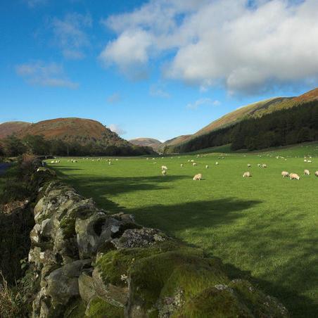
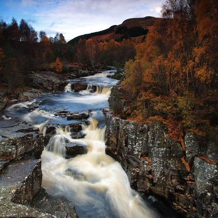
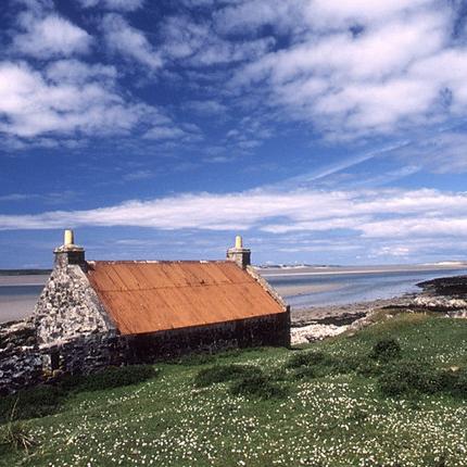
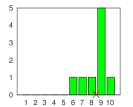
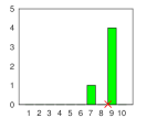
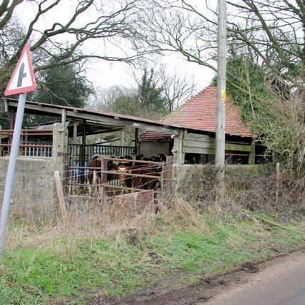
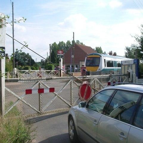
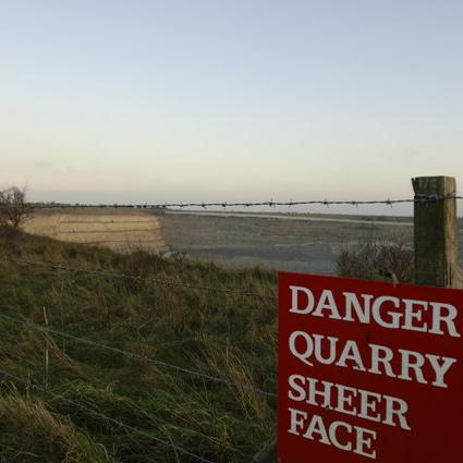
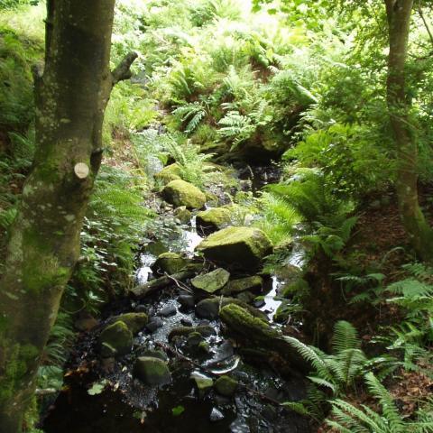
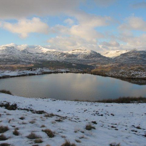
We apply our work to a database of 185,548 images and associated natural beauty rating histograms. Each image in the dataset was rated at least five times. We refer to this set of images as the ScenicOrNot (SoN) dataset. In addition to retaining the rating distribution and average rating, we partition the set of images into “scenic” (average rating above 7.0) and “non-scenic” (average rating below 3.0) subgroups. Figure 2 shows sample images from the dataset. In the remainder of this section, we explore image properties that may be associated with scenicness, including: text annotations, color statistics, and semantic image attributes.
2.1 Image Captions
Like most images hosted on image sharing sites, the SoN images have associated metadata, including a title and caption. For example, the image in Figure 1 (top, left) is titled From Troutbeck Tongue and has the following caption: “Looking over the cairn down Trout Beck. Windermere and the sea in the distance”. For all of the images in the SoN dataset, we analyzed the title and captions to explore whether these associated text annotations are correlated with scenicness.
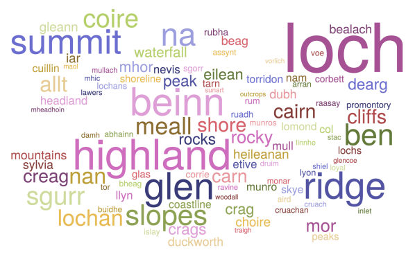
Using the scenic and non-scenic subsets, we compute the relative term frequency for each of the extracted words. Figure 3 shows a word cloud of the most frequent 100 extracted terms from scenic images, where the size of the word represents the relative frequency. While some of the terms (e.g., “ridge”, “cliffs”, “summit”) may universally correlate with scenicness, other terms, such as “loch”, “na”, and “beinn” reflect the fact the data originates from Great Britain. Conversely, example terms that are negatively correlated with scenicness include “road”, “lane”, “house”, and “railway”.
2.2 Color Distributions
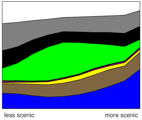
The images in Figure 2 and terms in Figure 3 suggest that images with blue skies, green fields, water, and other natural features tend to be rated as more scenic. For this analysis, we computed the distribution of quantized color values, using the approach of Van De Weijer et al. [30], as a function of the average scenicness rating of the SoN image set. Figure 4 shows the distribution, where we see blue overrepresented in scenic images and, conversely, black and gray overrepresented in non-scenic images.
2.3 Scene Semantics
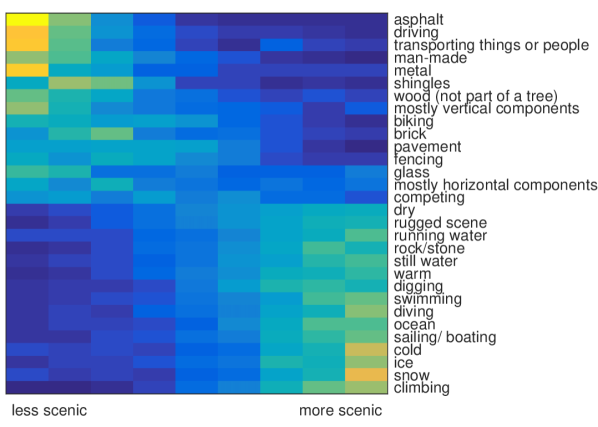
For each image, we compute SUN attributes [20], a set of 102 discriminative scene attributes spanning several types (e.g., function, materials). Figure 5 shows an occurrence matrix for a subset of attributes correlated with image scenicness. Attributes such as “asphalt”, “man-made”, and “transporting things or people” occur often in less scenic images, suggesting that urban environments are more typical of images with low scenicness. In contrast, attributes such as “ocean”, “climbing”, and “sailing/boating” occur more often in the most scenic images.
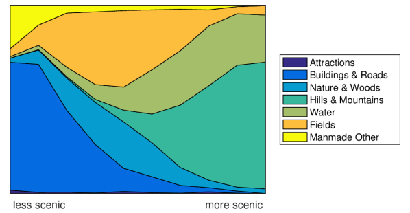
Similarly, we compared scenicness to the scene categorizations generated by the Places [40] convolutional neural network. Of the 205 Places scene classes (e.g., “airplane cabin”, “hotel room”, “shed”), 135 describe outdoor categories. We aggregate the outdoor classes into seven higher-level scene categories (similar to Runge et al. [24]), such as “buildings and roads”, “nature and woods”, and “hills and mountains”. Each image is classified using Places into one of these high-level categories. Figure 6 shows the frequency of each category as a function of the average user-provided rating of SoN images. The trend follows previously observed patterns; on the whole, images containing natural features, such as hills, mountains, and water, are rated as more scenic than images containing buildings, roads, and other man-made constructs.
2.4 Summary
This analysis shows that scenicness is related to both low-level image characteristics, such as color, and semantic properties, such as extracted attributes and scene categories. This suggests that it is possible to estimate scenicness from images. In the following section, we propose a method for directly estimating image scenicness from raw pixel values.
3 Predicting Image Scenicness
We use a deep convolutional neural network (CNN) to address the task of automatically estimating the scenicness of an image. Following other approaches (e.g., [31, 35]), we partition the output space and treat this prediction as a discrete labeling task where the output layer corresponds to the integer ratings (i.e., ) of scenicness. We represent our CNN as a function, , where is an image and the output is a probability distribution over the 10 scenicness levels. We consider multiple loss functions during training to best capture the distribution in human ratings of scenicness for a given image.
The baseline approach follows recent work (e.g., [36]), which trains a model to predict a single value. For this variant, each image is associated with the label corresponding to the mean human rating, rounded to the nearest integer value, . Training involves minimizing the typical cross-entropy loss:
| (1) |
where is the number of training examples.
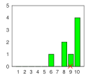
The baseline approach assumes a single underlying value for scenicness. However, as shown in Figure 2, for many images, there may be high variability in the ratings. In these cases, the mean scenicness may not serve as a representative value. So, instead of directly predicting the mean scenicness, we train the model to predict the human rating distribution for a particular image. For this variant, we treat the normalized human ratings as a target distribution and train the model to predict this distribution directly, by minimizing the cross-entropy loss:
| (2) |
where is the proportion of ratings for image .
However, the previous formulation assumes a large number of ratings so that approaches the true distribution. In our case, this assumption does not hold. As an alternative to predicting the mean scenicness or the empirical scenicness distribution, we model the set of ratings for an image as a sample from a multinomial distribution. Each training example is associated with a set of (potentially noisy) labels , where is the set of ratings for image . This results in the following loss:
| (3) |
where is the total number of ratings for image .
3.1 Comparison with Human Ratings
We evaluate our scenicness predictions using the SoN dataset. We reserved 1,413 images that have at least ten ratings as test cases for evaluation, with the remaining data used for training and validation. For predicting scenicness, we modify the GoogleNet architecture [29] with weights initialized from the Places network [40]. We selected this CNN because it had been trained for the related task of outdoor scene classification; however, our methods could be applied to other related architectures or trained from scratch with sufficient data. Our implementation uses the Caffe [8] deep learning toolbox. For training, we randomly initialize the last layer weights and optimize parameters using stochastic gradient descent with a base learning rate of and a mini-batch size of 40 images. Roughly 10% of the training data is reserved for validation. All trained models, including example code, are available at our project website.222http://cs.uky.edu/~scott/research/scenicness/
We refer to the three models as: (1) Average, the baseline approach that predicts the mean scenicness (Equation 1); (2) Distribution, the model that minimizes cross-entropy loss to the normalized distribution of human ratings (Equation 2); and (3) Multinomial, which maximizes the multinomial log-likelihood (Equation 3). We compare performance on two tasks: (1) predicting the average human rating and (2) predicting the distribution of ratings for a given image.
The output of each network is a posterior probability for each integer rating for a given input image. To evaluate the average user predictions, we consider the order of the predictions, ranked by posterior probability and use the information retrieval metric, Normalized Discounted Cumulative Gain (nDCG), which penalizes “out of order” posterior probabilities, given the ground-truth rating. The second column of Table 1 shows the nDCG scores for each of the three models. Overall, the models trained using different loss functions performed similarly well under this evaluation metric.
| Loss | Metric | |
|---|---|---|
| nDCG | K-S | |
| Average | .9780 | 14.8% |
| Distribution | .9678 | 50.0% |
| Multinomial | .9745 | 58.4% |
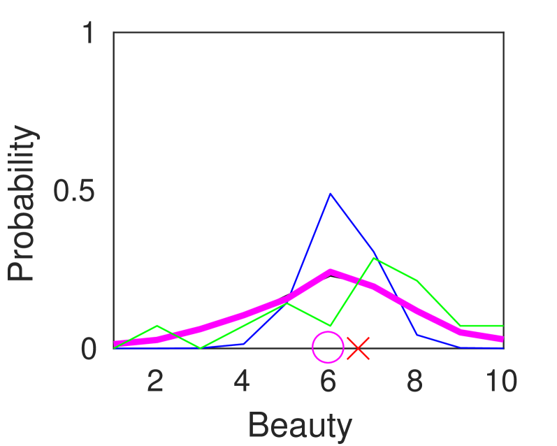
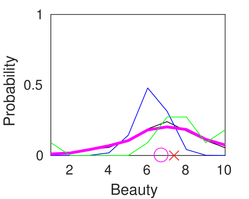
For the task of predicting the distribution of ratings for a given image, the performance of the models diverged. We take a hypothesis testing approach and consider whether or not the set of human ratings could be drawn from the distribution represented by the output probabilities of the CNN. For this, we applied the one-sample Kolmogorov-Smirnov (K-S) test with a non-parametric distribution and computed the proportion of testing images for which the human ratings come from the posterior distribution at the 5% significance level. The last column of Table 1 shows the percentage of testing images that matched the predicted distribution. The models trained using distribution of ratings, Distribution and Multinomial, significantly outperform the model trained on average rating, with Multinomial showing the best performance.
|
|
|
|
|
|
|
|
|
|
|
|
|
|
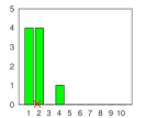
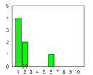
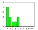
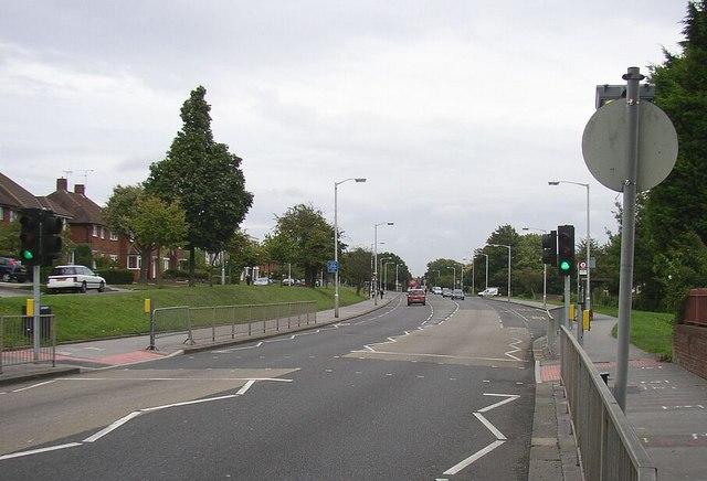
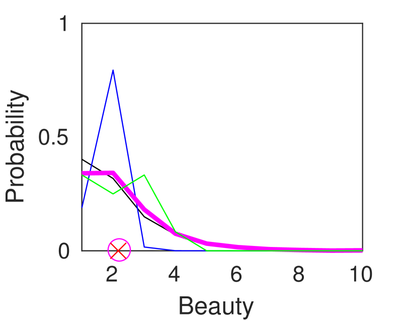
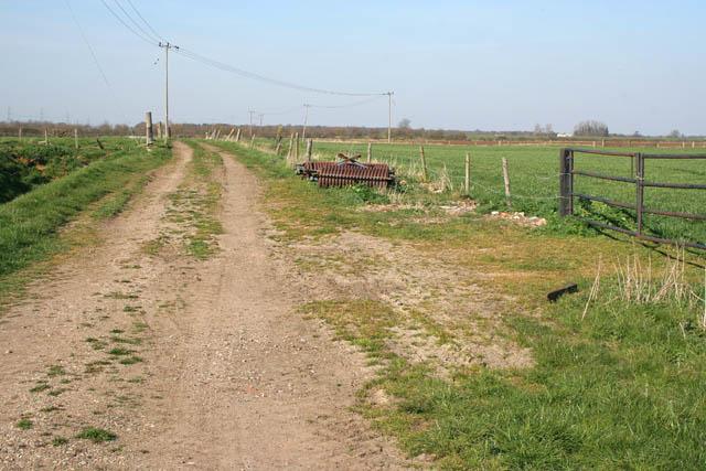
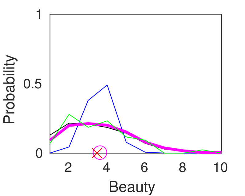
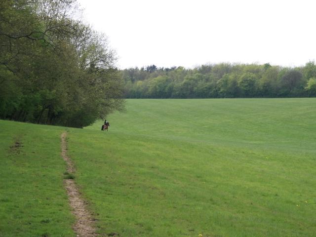
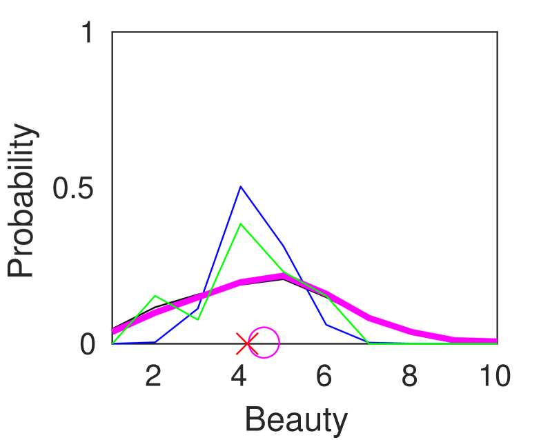
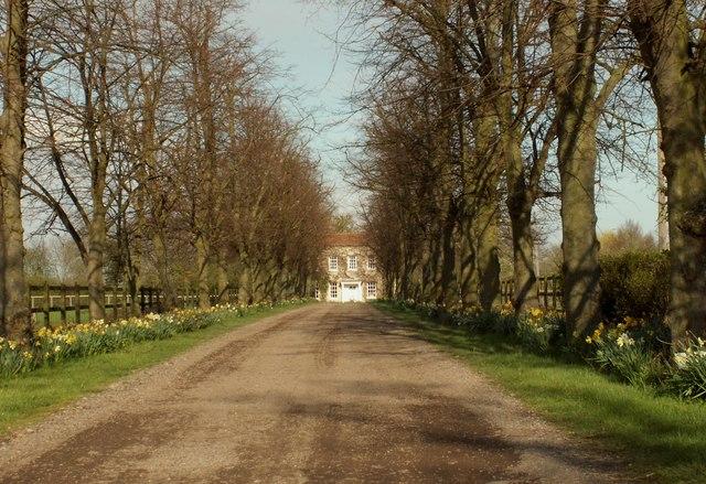
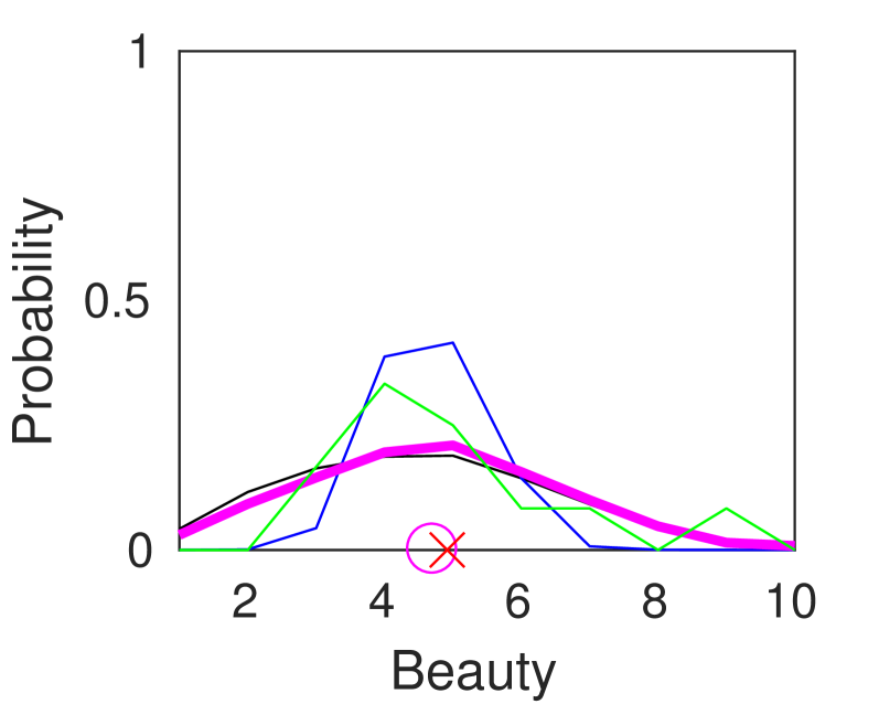
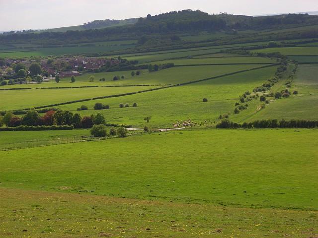
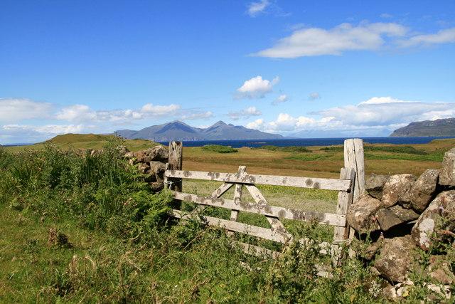
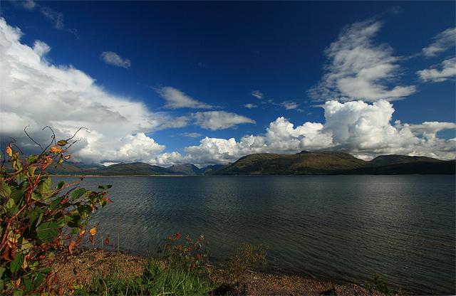
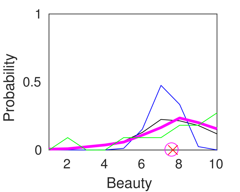
Figure 7 visualizes these results qualitatively. Several example images are shown alongside the distribution of human ratings (green) and predictions from the three models. In general, the results follow the quantitative analysis. The Multinomial method better captures human uncertainty as compared to the other methods. For example, in Figure 7 (row 1), the baseline approach, Average, provides a much higher posterior probability for a rating of 2 than the distribution of humans ratings. Comparatively, Multinomial is more consistent with human ratings and closer to the average user predictions. For the remaining experiments, the Multinomial model is used unless otherwise specified.
3.2 Receptive Fields of Natural Beauty
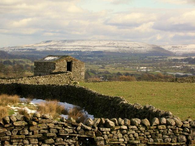
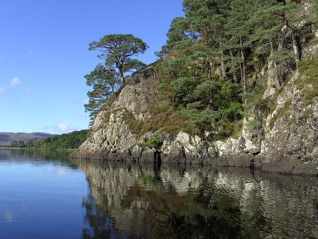
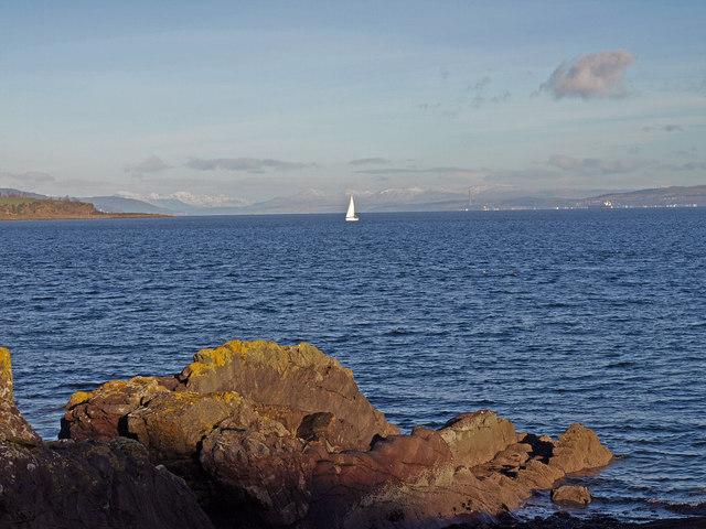
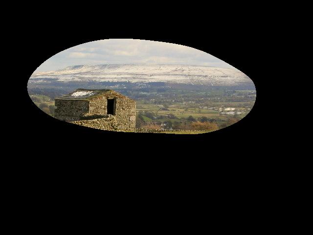
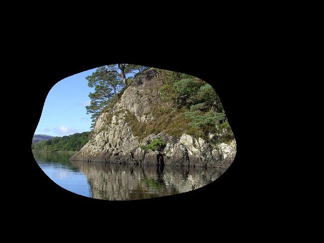
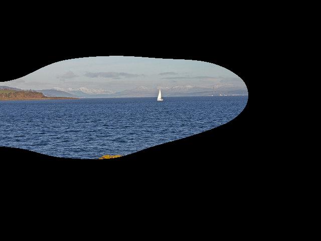
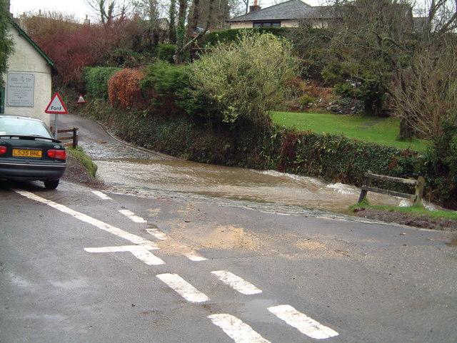
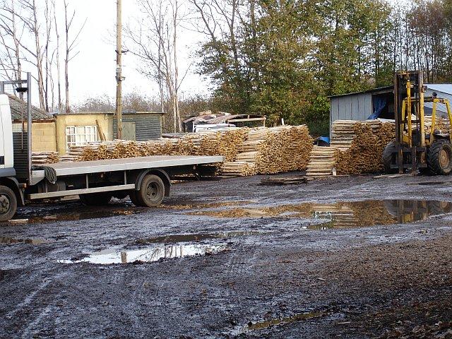
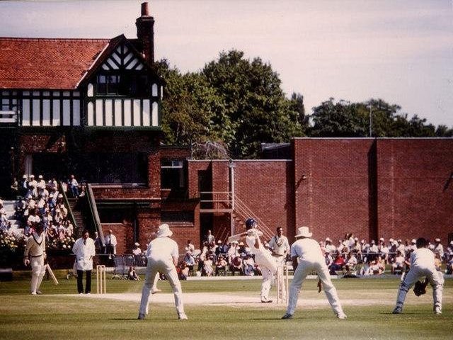
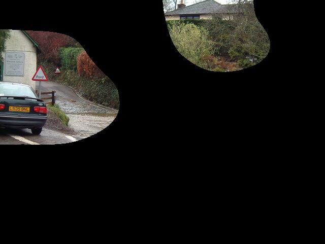
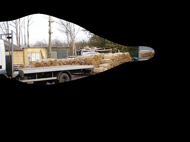
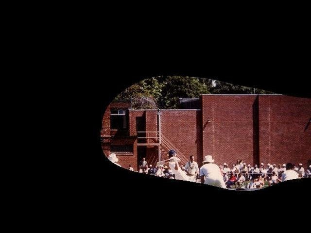
For additional insight into our scenicness predictions, following Zhou et al. [39], we apply receptive field analysis to highlight the regions of the image that are most salient in generating the output distribution. Briefly, the approach computes the differences in output predictions for a given image with a small (i.e., ) mask applied. Using a sliding window approach, the prediction differences (compared to the unmasked image) are computed on a grid across the image. A large difference signifies the masked region plays a significant role in the output prediction. This process leads to a saliency map over the input image. For visualization purposes, we represent the map as a binary mask (thresholded at 0.6). Figure 8 shows several examples of this analysis. Each pair of images shows the input and the image regions with the most contribution to the (high or low) scenicness score. In most cases, the receptive fields match the intuition and semantic analysis of scenicness. Regions containing water, trees, and horizons contribute to scenicness, while man-made objects, such as buildings and cars, contribute to non-scenicness.
3.3 Scenicness-Aware Image Cropping
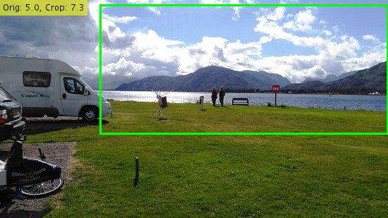
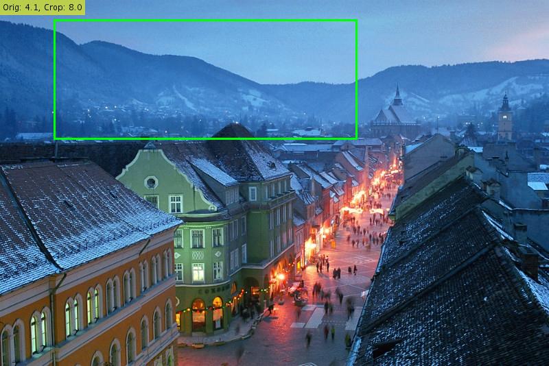
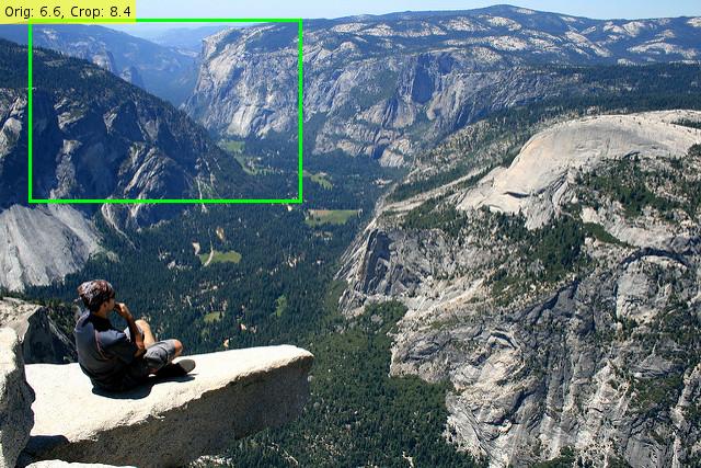
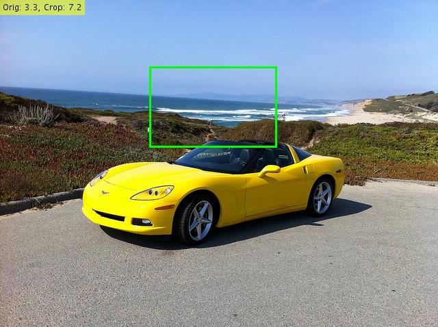
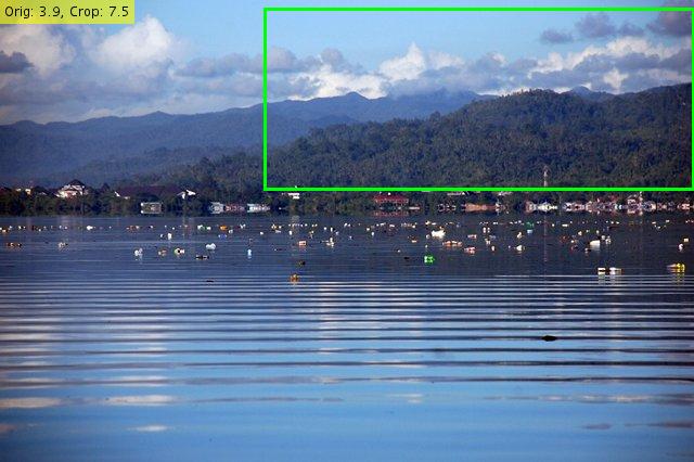
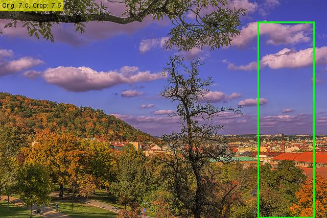
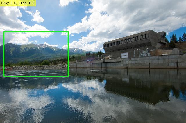
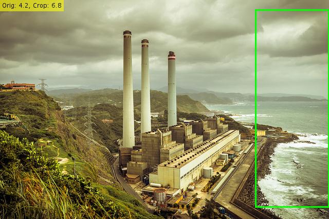
The previous experiment shows that components within a given image contribute differently to the overall scenicness. For this experiment, we solve for the image crop that maximizes scenicness. This approach follows the style of previous methods for content-aware image processing (e.g., seam carving for image resizing [2]). We used constrained Bayesian optimization [5] to solve for the position and size of the maximally scenic image crop, where scenicness is measured as the weighted average prediction from the Multinomial network. Figure 9 shows representative examples. In some cases, cropping improved the scenicness scores greatly. For example, in the top image in Figure 9, cropping out the vehicles increased the predicted scenicness from 5.0 to 7.3.

4 Mapping Image Scenicness
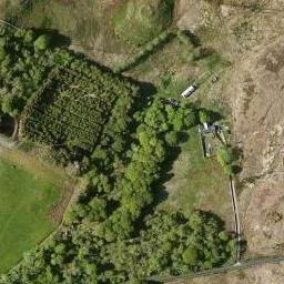
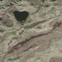
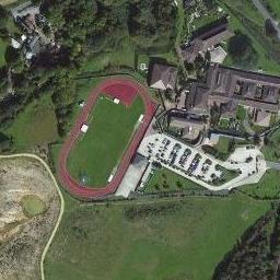
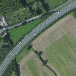
The previous sections considered scenicness as a property of an image. Here, we consider scenicness as a property of geographic locations and propose a novel approach for estimating scenicness over a large spatial region. We extend our approach for single-image estimation to incorporate overhead imagery. The result is a dense, high-resolution map that reflects the scenicness for every location in a region of interest. Such a map could, for example, be used to provide driving directions optimized for “sight seeing” [23, 24] or suggest places to go for a walk [22].
We consider geotagged images as noisy samples of the underlying geospatial scenicness function. The challenge is that ground-level imagery is sparsely distributed, especially away from major urban areas and tourist attractions. This means that methods which estimate maps using only ground-level imagery [1, 21, 36] typically generate either low-resolution or noisy maps.
To deal with the problem of interpolating sparse examples over large spatial regions, we apply a cross-view training and mapping approach. Cross-view methods [14, 33, 38] incorporate both ground-level and overhead viewpoints and take advantage of the fact that, while ground-level images are spatially sparse, overhead imagery is available at a high-resolution in most locations. Jointly reasoning about ground-level and overhead imagery has become popular in recent years. Luo et al. [17] use overhead imagery to perform better event recognition by fusing complementary views. Lin et al. [13, 14] introduce the problem of cross-view geolocalization, where an overhead image reference database is used to support ground-level image localization by learning a feature mapping between the two viewpoints. Workman et al. [32, 33] study the geo-dependence of image features and propose a cross-view training approach.
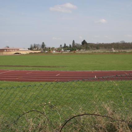
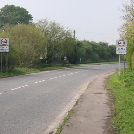
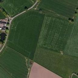
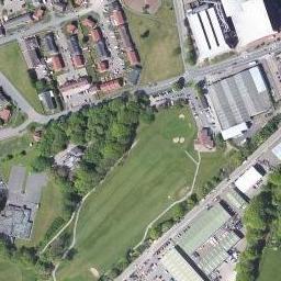
To support these efforts, we extend the ScenicOrNot (SoN) dataset to incorporate overhead images. Specifically, for each geotagged, ground-level SoN image, we obtained a orthorectified overhead image centered at that location from Bing Maps (zoom level 16, which is 2.4 meters/pixel). Figure 10 shows co-located pairs of ground-level and overhead images from the Cross-View ScenicOrNot (CVSoN) dataset. The dataset is available at our project website.2
4.1 Cross-View Mapping
To predict the scenicness of an overhead image even though labeled overhead images are not available, we apply a cross-view training strategy; instead of predicting the scenicness of the overhead image, we predict the scenicness of a ground-level image captured at the same location. We use the same network architecture and training methods as with the ground-level network, with two changes: (1) overhead (instead of ground-level) images are used as input and (2) the weights are initialized with those learned from the ground-level network. Similar to our ground-level network, after training, the output of this overhead image network is a distribution over scenicness ratings.
While using overhead images as input may address the issue of sparse spatial coverage of ground-level imagery, an overhead-only network may miss, for example, scenic views hidden amongst dense urban areas. To address this issue, we introduce a novel variant to the cross-view approach for combining ground-level and overhead imagery to estimate the scenicness of a query location. This is similar to our framework for estimating geospatial functions [34].
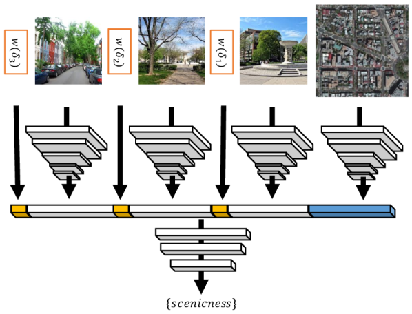
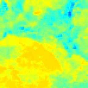
Figure 11 shows an overview of our hybrid cross-view approach. For a given query location, , consider the co-located overhead image, set of the closest ground-level images, and the distances of the ground-level images to the query location, . For the images, we can compute scenicness features using the existing ground and overhead networks. For the hybrid approach, we learn and predict scenicness from the fused features (overhead image features, ground-level features, weighted distances) using a small feed-forward network, with three hidden layers containing 100, 50, and 25 neurons, respectively. The activation function on the internal nodes is the hyperbolic tangent sigmoid. The network weights are regularized using an loss with a weight of . The output is the predicted distribution of ratings for a ground-level image taken at the input location. We refer to this as the Cross-View Hybrid (CVH) network.
4.2 Mapping the Scenicness of Great Britain
To evaluate CVH, the CVSoN dataset is divided as before, with the same 1,413 ground-level images (with at least 10 ratings) held out for testing. For CVH, the test input includes the co-located overhead image. We compare against two baseline methods for constructing dense maps of visual properties:
-
•
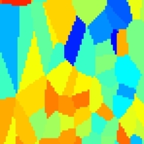
1NN: return the prediction from the ground-level image closest to the query location; and
-
•
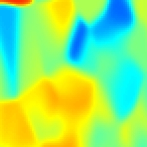
LWA: return the locally weighted average prediction of neighboring ground-level images with a Gaussian kernel ( degrees).
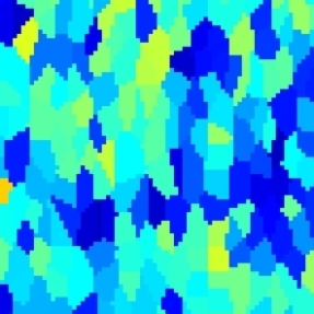
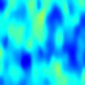
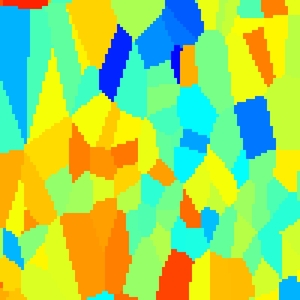
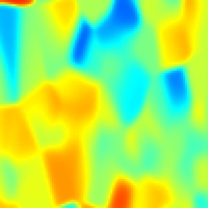
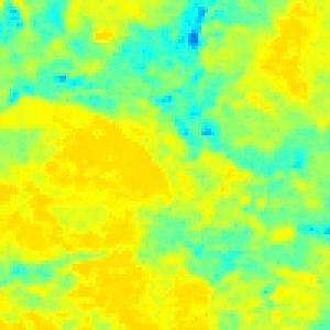
To compare our methods, we formulate a binary classification task to determine if a given test image is above or below a scenicness rating of 7. Table 2 shows the results for each method as the area under the curve (AUC) of the ROC curve computed from the output distributions. The results show that including orthographic overhead imagery improves the resulting predictions.
| Method | 1NN | LWA | CVH |
| AUC | 64.38% | 66.86% | 68.51% |
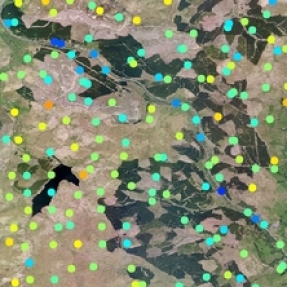
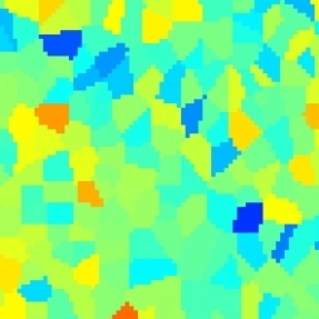
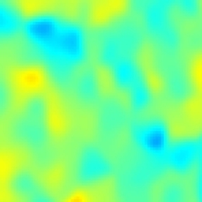
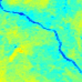
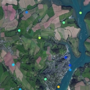
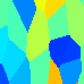
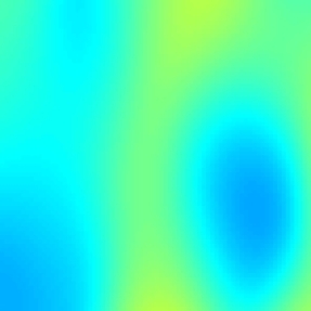
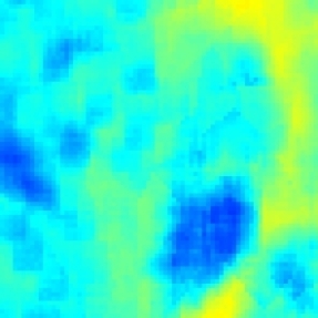
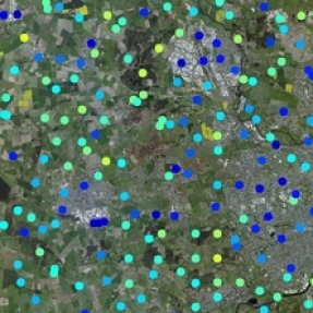
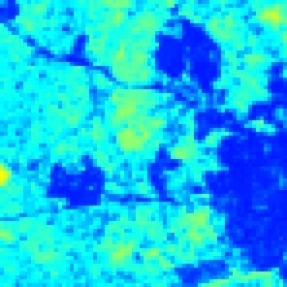
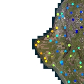
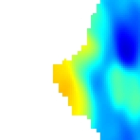
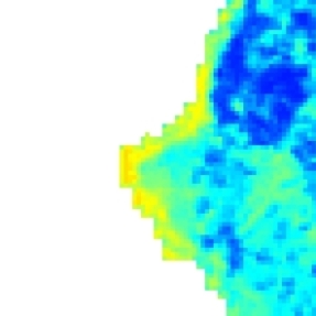
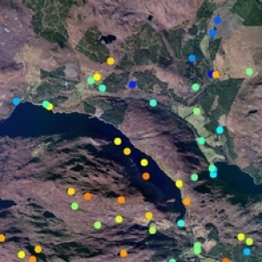
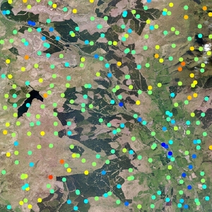
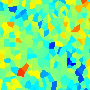
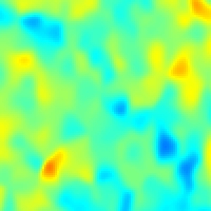
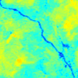
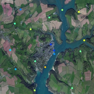
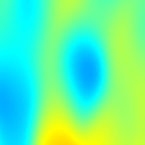
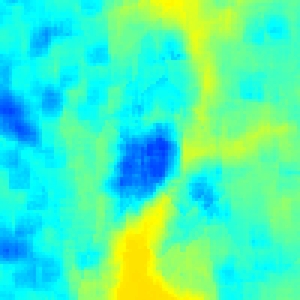
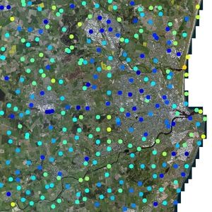
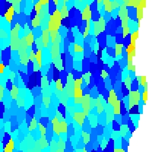
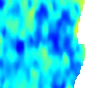
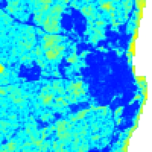
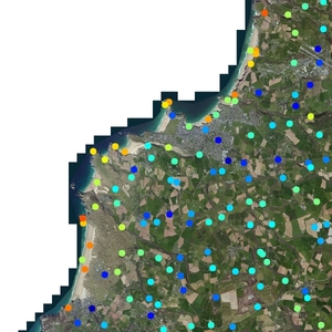
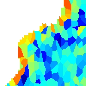
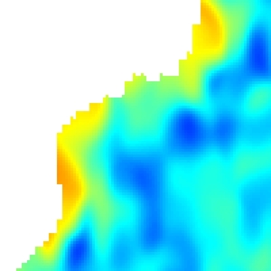
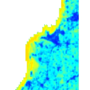
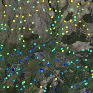
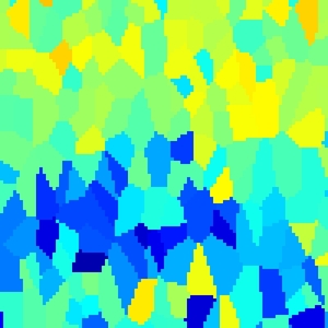
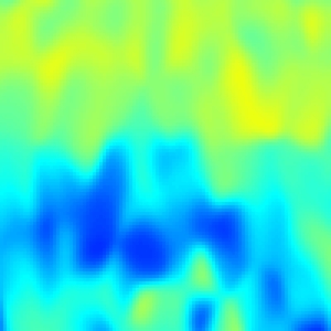
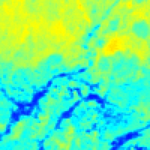
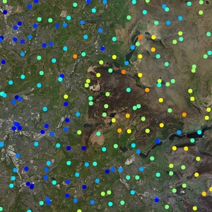
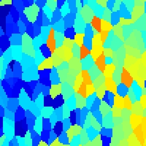
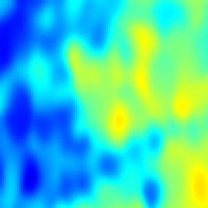
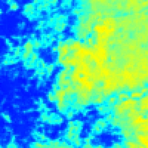
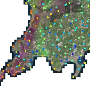
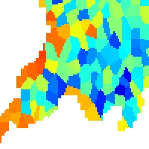
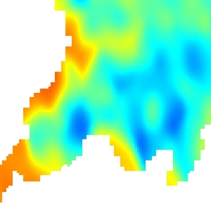
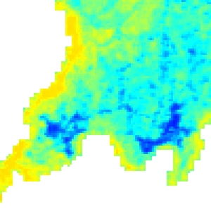
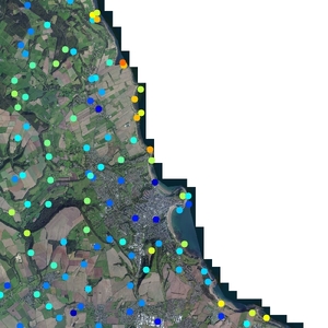
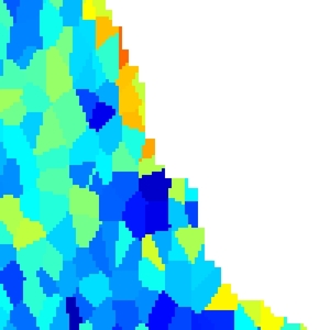
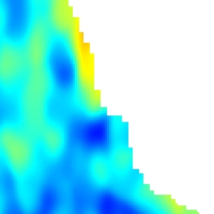
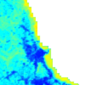
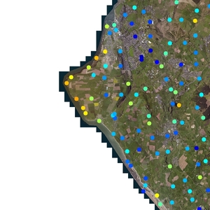
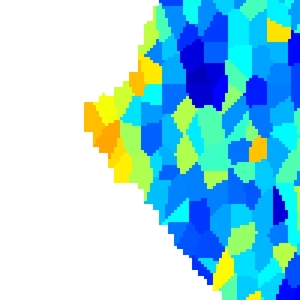
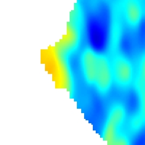
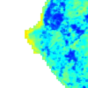
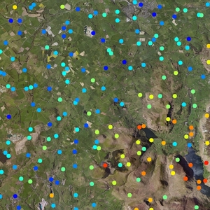
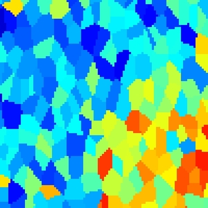
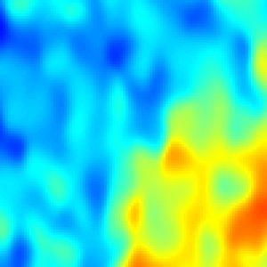
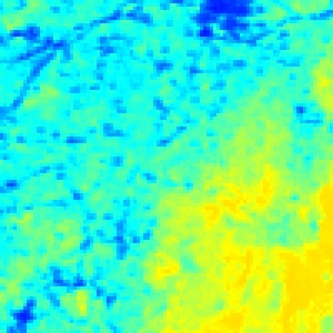
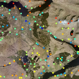
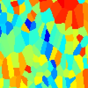
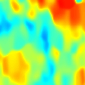
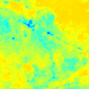
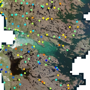
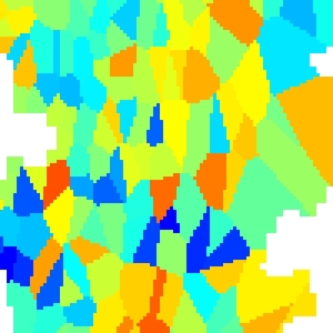
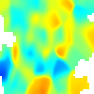
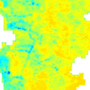
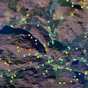
These results are supported qualitatively in Figure 12, which shows scenicness maps for several regions around Great Britain. We observe that by including overhead imagery we are able to construct a significantly more accurate map than purely interpolating scenicness estimates obtained from ground-level images alone. The maps created using only ground-level images (e.g., 1NN, LWA) are susceptible to both underprediction (e.g., no nearby scenic ground-level images) and overprediction (e.g., a single nearby scenic image with a narrow field of view). On the other hand, the cross-view approach can be more robust against these types of mispredictions due to effectively averaging across many images (by marginalizing through the overhead imagery), not just those in the nearby area.
| ROI | 1NN | LWA | CVH |
|---|---|---|---|
 |
 |
 |
 |
 |
 |
 |
 |
 |
 |
 |
 |
 |
 |
 |
 |
 |
 |
 |
 |
5 Conclusions
We explored the concept of natural beauty as it pertains to outdoor imagery. Using a dataset containing hundreds of thousands of ground-level images rated by humans, we showed it is possible to quantify scenicness, from both ground-level and overhead viewpoints. To our knowledge, this is the first time a combination of overhead and geotagged ground-level imagery has been used to map the scenicness of a region. The resulting maps are higher-resolution than those constructed by previous approaches and can be quickly computed. Such methods have significant practical importance to many areas, including: tourism, transportation routing, and environmental monitoring.
Acknowledgments
We thank our colleagues, Tawfiq Salem and Zachary Bessinger, for their help, and Robert Pless and Mirek Truszczynski for their insightful advice. We gratefully acknowledge the support of NSF CAREER grant IIS-1553116 and a Google Faculty Research Award.
References
- [1] S. M. Arietta, A. A. Efros, R. Ramamoorthi, and M. Agrawala. City forensics: Using visual elements to predict non-visual city attributes. IEEE Transactions on Visualization and Computer Graphics, 20(12):2624–2633, 2014.
- [2] S. Avidan and A. Shamir. Seam carving for content-aware image resizing. ACM Transactions on Graphics, 26(3):10, 2007.
- [3] A. Chandrasekaran, A. K. Vijayakumar, S. Antol, M. Bansal, D. Batra, C. Lawrence Zitnick, and D. Parikh. We are humor beings: Understanding and predicting visual humor. In IEEE Conference on Computer Vision and Pattern Recognition, 2016.
- [4] A. Deza and D. Parikh. Understanding image virality. In IEEE Conference on Computer Vision and Pattern Recognition, 2015.
- [5] J. Gardner, M. Kusner, K. Q. Weinberger, J. Cunningham, and Z. Xu. Bayesian optimization with inequality constraints. In International Conference on Machine Learning, 2014.
- [6] P. Isola, J. Xiao, A. Torralba, and A. Oliva. What makes an image memorable? In IEEE Conference on Computer Vision and Pattern Recognition, 2011.
- [7] M. Jas and D. Parikh. Image specificity. In IEEE Conference on Computer Vision and Pattern Recognition, 2015.
- [8] Y. Jia, E. Shelhamer, J. Donahue, S. Karayev, J. Long, R. Girshick, S. Guadarrama, and T. Darrell. Caffe: Convolutional architecture for fast feature embedding. In ACM International Conference on Multimedia, 2014.
- [9] S. Karayev, M. Trentacoste, H. Han, A. Agarwala, T. Darrell, A. Hertzmann, and H. Winnemoeller. Recognizing image style. In British Machine Vision Conference, 2014.
- [10] Y. Ke, X. Tang, and F. Jing. The design of high-level features for photo quality assessment. In IEEE Conference on Computer Vision and Pattern Recognition, 2006.
- [11] P.-Y. Laffont, Z. Ren, X. Tao, C. Qian, and J. Hays. Transient attributes for high-level understanding and editing of outdoor scenes. ACM Transactions on Graphics (SIGGRAPH), 33(4), 2014.
- [12] J. H. Langlois, L. Kalakanis, A. J. Rubenstein, A. Larson, M. Hallam, and M. Smoot. Maxims or myths of beauty? a meta-analytic and theoretical review. Psychological bulletin, 126(3):390, 2000.
- [13] T.-Y. Lin, S. Belongie, and J. Hays. Cross-view image geolocalization. In IEEE Conference on Computer Vision and Pattern Recognition, 2013.
- [14] T.-Y. Lin, Y. Cui, S. Belongie, and J. Hays. Learning deep representations for ground-to-aerial geolocalization. In IEEE Conference on Computer Vision and Pattern Recognition, 2015.
- [15] X. Lu, Z. Lin, H. Jin, J. Yang, and J. Z. Wang. Rapid: Rating pictorial aesthetics using deep learning. In ACM International Conference on Multimedia, 2014.
- [16] X. Lu, C. Wang, J.-M. Yang, Y. Pang, and L. Zhang. Photo2trip: generating travel routes from geo-tagged photos for trip planning. In ACM International Conference on Multimedia, 2010.
- [17] J. Luo, J. Yu, D. Joshi, and W. Hao. Event recognition: viewing the world with a third eye. In ACM International Conference on Multimedia, 2008.
- [18] Y. Luo and X. Tang. Photo and video quality evaluation: Focusing on the subject. In European Conference on Computer Vision, 2008.
- [19] D. A. McGranahan. Natural amenities drive rural population change. Technical report, United States Department of Agriculture, Economic Research Service, 1999.
- [20] G. Patterson and J. Hays. Sun attribute database: Discovering, annotating, and recognizing scene attributes. In IEEE Conference on Computer Vision and Pattern Recognition, 2012.
- [21] L. Porzi, S. Rota Bulò, B. Lepri, and E. Ricci. Predicting and understanding urban perception with convolutional neural networks. In ACM International Conference on Multimedia, 2015.
- [22] D. Quercia, L. M. Aiello, R. Schifanella, and A. Davies. The digital life of walkable streets. In International World Wide Web Conference, 2015.
- [23] D. Quercia, R. Schifanella, and L. M. Aiello. The shortest path to happiness: Recommending beautiful, quiet, and happy routes in the city. In ACM Conference on Hypertext and Social Media, 2014.
- [24] N. Runge, P. Samsonov, D. Degraen, and J. Schöning. No more autobahn!: Scenic route generation using googles street view. In International Conference on Intelligent User Interfaces, 2016.
- [25] C. I. Seresinhe, H. S. Moat, and T. Preis. Quantifying scenic areas using crowdsourced data. Environment and Planning B: Urban Analytics and City Science, 2017.
- [26] C. I. Seresinhe, T. Preis, and H. S. Moat. Quantifying the impact of scenic environments on health. Scientific Reports, 5, 2015.
- [27] C. I. Seresinhe, T. Preis, and H. S. Moat. Using deep learning to quantify the beauty of outdoor places. Royal Society Open Science, 4(7), 2017.
- [28] H.-H. Su, T.-W. Chen, C.-C. Kao, W. H. Hsu, and S.-Y. Chien. Scenic photo quality assessment with bag of aesthetics-preserving features. In ACM International Conference on Multimedia, 2011.
- [29] C. Szegedy, W. Liu, Y. Jia, P. Sermanet, S. Reed, D. Anguelov, D. Erhan, V. Vanhoucke, and A. Rabinovich. Going deeper with convolutions. In IEEE Conference on Computer Vision and Pattern Recognition, 2015.
- [30] J. Van De Weijer, C. Schmid, J. Verbeek, and D. Larlus. Learning color names for real-world applications. IEEE Transactions on Image Processing, 18(7):1512–1523, 2009.
- [31] T. Weyand, I. Kostrikov, and J. Philbin. Planet-photo geolocation with convolutional neural networks. In European Conference on Computer Vision, 2016.
- [32] S. Workman and N. Jacobs. On the location dependence of convolutional neural network features. In IEEE/ISPRS Workshop: Looking from above: When Earth observation meets vision, 2015.
- [33] S. Workman, R. Souvenir, and N. Jacobs. Wide-area image geolocalization with aerial reference imagery. In IEEE International Conference on Computer Vision, 2015.
- [34] S. Workman, M. Zhai, D. J. Crandall, and N. Jacobs. A unified model for near and remote sensing. In IEEE International Conference on Computer Vision, 2017.
- [35] S. Workman, M. Zhai, and N. Jacobs. Horizon lines in the wild. In British Machine Vision Conference, 2016.
- [36] L. Xie and S. Newsam. Im2map: deriving maps from georeferenced community contributed photo collections. In ACM SIGMM International Workshop on Social media, 2011.
- [37] C.-H. Yeh, Y.-C. Ho, B. A. Barsky, and M. Ouhyoung. Personalized photograph ranking and selection system. In ACM International Conference on Multimedia, 2010.
- [38] M. Zhai, Z. Bessinger, S. Workman, and N. Jacobs. Predicting ground-level scene layout from aerial imagery. In IEEE Conference on Computer Vision and Pattern Recognition, 2017.
- [39] B. Zhou, A. Khosla, A. Lapedriza, A. Oliva, and A. Torralba. Object detectors emerge in deep scene cnns. In International Conference on Learning Representations, 2014.
- [40] B. Zhou, A. Lapedriza, J. Xiao, A. Torralba, and A. Oliva. Learning deep features for scene recognition using places database. In Advances in Neural Information Processing Systems, 2014.
- [41] E. H. Zube, J. L. Sell, and J. G. Taylor. Landscape perception: research, application and theory. Landscape planning, 9(1):1–33, 1982.
Supplemental Material : Understanding and Mapping Natural Beauty
This document contains additional details and experiments related to our methods.
1 Exploring Image Scenicness
1.1 Uncertainty in Scenicness Scores
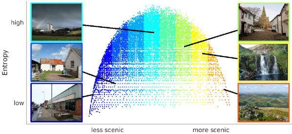
Figure S1 shows a scatter plot of Shannon entropy, computed per image from ratings, versus scenicness, for all images in the ScenicOrNot (SoN) dataset. Each dot represents an image and is colored by the average beauty score. Unsurprisingly, the images that are rated the least and most scenic have higher consistency in their scenicness ratings.
1.2 Image Captions
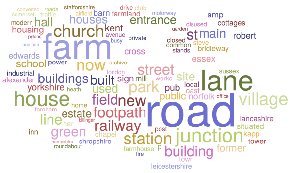
Figure S2 shows a word cloud of the most frequent 100 extracted terms from captions and titles associated with non-scenic images in SoN (average rating below 3.0), where the size of the word represents the relative frequency. Example terms that are negatively correlated with scenicness include “road”, “lane”, “house”, and “railway”.
2 Experiments
2.1 Scenicness-Aware Image Cropping
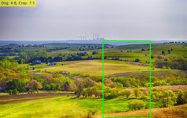
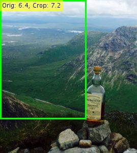
Figure S3 shows additional examples of applying our methods for scenicness-aware image processing. In each image, the inset shows the change in scenicness from the full image to the cropped image.
 |
 |
 |
 |
 |
 |
 |
 |
2.2 Mapping Scenicness
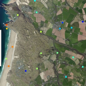
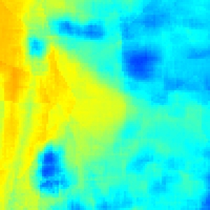
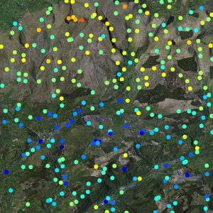
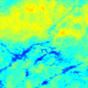
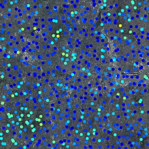
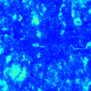
Our method is applicable for generating maps of scenicness at widely varying spatial scales. Figure S4 shows three examples of fine-grained high-resolution maps of scenicness from regions of different sizes around Great Britain. Figure S4 (top) shows a stretch of coast near Holywell, a coastal village in north Cornwall, England. Figure S4 (middle) shows a map centered over Caehopkin, a village in Powys, Wales. Caehopkin sits between Abercraf and Coelbren in the Swansea Valley and lies on the border of the Brecon Beacons National Park to the north. Figure S4 (bottom) shows a map of Greater London. Figure S5 and Figure S6 show additional maps of scenicness computed using our method, alongside several baseline approaches. In all cases, Cross-View Hybrid (CVH) combines overhead imagery and nearby ground-level images to more accurately identify scenic and non-scenic locations.
| ROI | CVH |
|---|---|
 |
 |
 |
 |
 |
 |
| ROI | 1NN | LWA | CVH |
|---|---|---|---|
 |
 |
 |
 |
 |
 |
 |
 |
 |
 |
 |
 |
 |
 |
 |
 |
 |
 |
 |
 |
 |
 |
 |
 |
 |
 |
 |
 |
| ROI | 1NN | LWA | CVH |
|---|---|---|---|
 |
 |
 |
 |
 |
 |
 |
 |
 |
 |
 |
 |
 |
 |
 |
 |
 |
 |
 |
 |
 |
 |
 |
 |