Characterizing the maximum parameter of the total-variation denoising through the pseudo-inverse of the divergence

Abstract

We focus on the maximum regularization parameter for anisotropic total-variation denoising. It corresponds to the minimum value of the regularization parameter above which the solution remains constant. While this value is well know for the Lasso, such a critical value has not been investigated in details for the total-variation. Though, it is of importance when tuning the regularization parameter as it allows fixing an upper-bound on the grid for which the optimal parameter is sought. We establish a closed form expression for the one-dimensional case, as well as an upper-bound for the two-dimensional case, that appears reasonably tight in practice. This problem is directly linked to the computation of the pseudo-inverse of the divergence, which can be quickly obtained by performing convolutions in the Fourier domain.

I Introduction

We consider the reconstruction of a $d$-dimensional signal (in this study $d=1$ or $2$) from its noisy observation $y\!=\!x+w\!\in\!\mathbb{R}^{n}$ with $w\!\in\!\mathbb{R}^{n}$. Anisotropic TV regularization writes, for $\lambda>0$, as [1]

$$x^{\star}=\underset{x\in\mathbb{R}^{n}}{\operatorname{argmin}}\;\frac{1}{2}|\!|y-x|\!|_{2}^{2}+\lambda|\!|\nabla x|\!|_{1}$$ (1)

with $\nabla x\!\in\!\mathbb{R}^{dn}$ being the concatenation of the $d$ components of the discrete periodical gradient vector field of $x$, and $|\!|\nabla x|\!|_{1}\!=\!\sum_{i}|(\nabla x)_{i}|$ being a sparsity promoting term. The operator $\nabla$ acts as a convolution which writes in the one dimensional case ($d=1$)

$$\nabla=F^{+}\operatorname{diag}(K_{\rightarrow})F\quad\text{and}\quad\operatorname{div}=F^{+}\operatorname{diag}(K_{\leftarrow})F$$ (2)

where $\operatorname{div}=-\nabla^{\top}$ (where ^⊤ denotes the adjoint), $F:\mathbb{R}^{n}\mapsto\mathbb{C}^{n}$ is the Fourier transform, $F^{+}=\text{Re}[F^{-1}]$ is its pseudo-inverse and $K_{\rightarrow}\in\mathbb{C}^{n}$ and $K_{\leftarrow}\in\mathbb{C}^{n}$ are the Fourier transforms of the kernel functions performing forward and backward finite differences respectively. Similarly, we define in the two dimensional case ($d=2$)

$$\nabla =\begin{pmatrix}F^{+}&0\\ 0&F^{+}\end{pmatrix}\begin{pmatrix}\operatorname{diag}(K_{\downarrow})\\ \operatorname{diag}(K_{\rightarrow})\end{pmatrix}F$$ (3)

$$\quad\text{and}\quad\operatorname{div} =F^{+}\begin{pmatrix}\operatorname{diag}(K_{\uparrow})&\operatorname{diag}(K_{\leftarrow})\end{pmatrix}\begin{pmatrix}F&0\\ 0&F\end{pmatrix}$$ (4)

where $K_{\rightarrow}\in\mathbb{C}^{n}$ and $K_{\leftarrow}\in\mathbb{C}^{n}$ (resp. $K_{\downarrow}\in\mathbb{C}^{n}$ and $K_{\uparrow}\in\mathbb{C}^{n}$) perform forward and backward finite difference in the horizontal (resp. vertical) direction.

II General case

For the general case, the following proposition provides an expression of the maximum regularization parameter $\lambda_{\max}$ as the solution of a convex but non-trivial optimization problem (direct consequence of the Karush-Khun-Tucker condition).

Proposition 1.

Define for $y\in\mathbb{R}^{n}$,

$$\lambda_{\max}=\underset{\zeta\in\operatorname{Ker}[\operatorname{div}]}{\min}\;\|\operatorname{div}^{+}y+\zeta\,\|_{\infty}$$ (5)

where $\operatorname{div}^{+}$ is the Moore-Penrose pseudo-inverse of $\operatorname{div}$ and $\operatorname{Ker}[\operatorname{div}]$ its null space. Then, $x^{\star}=\frac{1}{n}{\mathds{1}}_{n}{\mathds{1}}_{n}^{\top}y$ if and only if $\lambda\geqslant\lambda_{\max}$.

III One dimensional case

In the 1d case, $\operatorname{Ker}[\operatorname{div}]=\operatorname{Span}({\mathds{1}}_{n})$ and thus the optimization problem can be solved by computing $\operatorname{div}^{+}$ in the Fourier domain, in $O(n\log n)$ operations, as shown in the next corollary.

Corollary 1.

For $d=1$, $\lambda_{\max}=\tfrac{1}{2}[\max(\operatorname{div}^{+}y)-\min(\operatorname{div}^{+}y)],$

where $$\operatorname{div}^{+}=F^{+}\operatorname{diag}(K_{\uparrow}^{+})F$$ (6)

and $$({K}_{\uparrow}^{+})_{i}=\left\{\begin{array}[]{ll}\frac{(K_{\uparrow})^{*}_{i}}{|(K_{\uparrow})_{i}|^{2}}&\text{if}\quad|(K_{\uparrow})_{i}|^{2}>0\\ 0&\text{otherwise}\end{array}\right.~{},$$ (9)

and ^∗ denotes the complex conjugate.

Note that the condition $|(K_{\uparrow})_{i}|^{2}>0$ is satisfied everywhere except for the zero frequency. In the non-periodical case, $\operatorname{div}$ is the incidence matrix of a tree whose pseudo-inverse can be obtained following [2].

IV Two dimensional case

In the 2d case, $\operatorname{Ker}[\operatorname{div}]$ is the orthogonal of the vector space of signals satisfying Kirchhoff’s voltage law on all cycles of the periodical grid. Its dimension is $n+1$. It follows that the optimization problem becomes much harder. Since our motivation is only to provide an approximation of $\lambda_{\max}$, we propose to compute an upper-bound in $O(n\log n)$ operations thanks to the following corollary.

Corollary 2.

For $d=2$, $\lambda_{\max}\leqslant\underbrace{\tfrac{1}{2}[\max(\operatorname{div}^{+}y)\!-\!\min(\operatorname{div}^{+}y)]}_{\lambda_{\mathrm{bnd}}},$

where $$\operatorname{div}^{+}=\begin{pmatrix}F^{+}&0\\ 0&F^{+}\end{pmatrix}\begin{pmatrix}\operatorname{diag}(\tilde{K}^{+}_{\uparrow})\\ \operatorname{diag}(\tilde{K}^{+}_{\leftarrow})\end{pmatrix}F,\quad\text{and}\quad$$ (10)

$$(\tilde{K}_{\uparrow}^{+})_{i} =\left\{\begin{array}[]{ll}\frac{(K_{\uparrow})^{*}_{i}}{|(K_{\uparrow})_{i}|^{2}+|(K_{\leftarrow})_{i}|^{2}}&\text{if}\quad|(K_{\uparrow})_{i}|^{2}+|(K_{\leftarrow})_{i}|^{2}>0\\ 0&\text{otherwise}\end{array}\right.~{},$$ (13)

$$(\tilde{K}_{\leftarrow}^{+})_{i} =\left\{\begin{array}[]{ll}\frac{(K_{\leftarrow})^{*}_{i}}{|(K_{\uparrow})_{i}|^{2}+|(K_{\leftarrow})_{i}|^{2}}&\text{if}\quad|(K_{\uparrow})_{i}|^{2}+|(K_{\leftarrow})_{i}|^{2}>0\\ 0&\text{otherwise}\end{array}\right.~{}.$$ (16)

Note that the condition $|(K_{\uparrow})_{i}|^{2}+|(K_{\leftarrow})_{i}|^{2}>0$ is again satisfied everywhere except for the zero frequency. Remark also that this result can be straightforwardly extended to the case where $d>2$.

V Results and discussion

Figure 3 and 3 provide illustrations of the computation of $\lambda_{\max}$ and $\lambda_{\mathrm{bnd}}$ on a 1d signal and a 2d image respectively. The convolution kernel is a simple triangle wave in the 1d case but is more complex in the 2d case. The operator $\operatorname{div}\operatorname{div}^{+}$ is in fact the projector onto the space of zero-mean signals, i.e., $\operatorname{Im}[\operatorname{div}]$. Figure 3 illustrates the evolution of $x^{\star}$ with respect to $\lambda$ (computed with the algorithm of [3]). Our upper-bound $\lambda_{\mathrm{bnd}}$ (computed in ${\sim}5$ms) appears to be reasonably tight ($\lambda_{\max}$ computed in ${\sim}25$s with [3] on Problem (5)).

Future work will concern the generalization of these results to other $\ell_{1}$ analysis regularization and to ill-posed inverse problems.

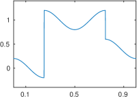
(a) $y$

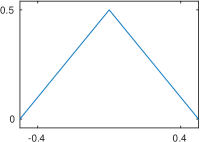
(b) $F^{+}K^{+}_{\uparrow}$

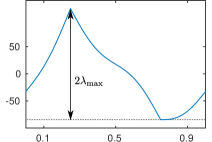
(c) $\operatorname{div}^{+}y$

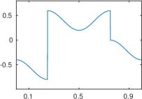
(d) $\operatorname{div}\operatorname{div}^{+}y$

Figure 1: (a) A 1d signal $y$. (b) The convolution kernel $F^{+}K^{+}_{\uparrow}$ that realizes the pseudo inversion of the divergence. (c) The signal $\operatorname{div}^{+}y$ on which we can read the value of $\lambda_{\max}$. (d) The signal $\operatorname{div}\operatorname{div}^{+}y$ showing that one can reconstruct $y$ from $\operatorname{div}^{+}y$ up to its mean component.

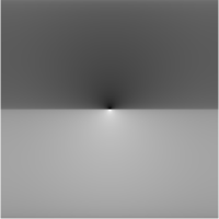
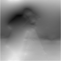
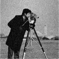
(a) $y$ (range [$0,255$])

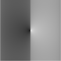
(b) $F^{+}\tilde{K}^{+}_{\uparrow}$, $F^{+}\tilde{K}^{+}_{\leftarrow}$ (in power scale)

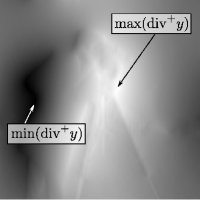
(c) $\operatorname{div}^{+}y$

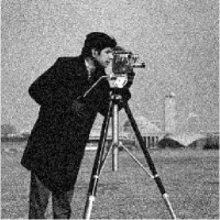
(d) $\operatorname{div}\operatorname{div}^{+}y$ (range [$-119,136$])

Figure 2: (a) A 2d signal $y$. (b) The convolution kernels $F^{+}K^{+}_{\uparrow}$ and $F^{+}\tilde{K}^{+}_{\leftarrow}$ that realizes the pseudo inversion of the divergence. (c) The absolute value of the two coordinates of the vector field $\operatorname{div}^{+}y$ on which we can read the upper-bound $\lambda_{\mathrm{bnd}}$ of $\lambda_{\max}$. (d) The image $\operatorname{div}\operatorname{div}^{+}y$ showing again that one can reconstruct $y$ from $\operatorname{div}^{+}y$ up to its mean component.

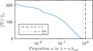
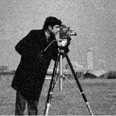
(a) $\lambda=10^{-3}\lambda_{\mathrm{bnd}}$

(b) $\lambda=10^{-2}\lambda_{\mathrm{bnd}}$

(c) $\lambda=\lambda_{\mathrm{bnd}}$

Figure 3: (a) Evolution of $|\!|\nabla x^{\star}\,|\!|_{\infty}$ as a function of $\lambda$. (b), (c), (d) Results $x^{\star}$ of the periodical anisotropic total-variation for three different values of $\lambda$.

References

[1]
L. I. Rudin, S. Osher, and E. Fatemi, “Nonlinear total variation based noise
removal algorithms,” Physica D: Nonlinear Phenomena, vol. 60, no. 1,
pp. 259–268, 1992.
[2]
R. Bapat, “Moore-penrose inverse of the incidence matrix of a tree,”
Linear and Multilinear Algebra, vol. 42, no. 2, pp. 159–167, 1997.
[3]
A. Chambolle and T. Pock, “A first-order primal-dual algorithm for convex
problems with applications to imaging,” J. Math. Imaging Vis.,
vol. 40, pp. 120–145, 2011.