Different models of gravitating Dirac fermions in optical lattices

Abstract

In this paper I construct the naive lattice Dirac Hamiltonian describing the propagation of fermions in a generic 2D optical metric for different lattice and flux-lattice geometries. First, I apply a top-down constructive approach that we first proposed in [Boada et al.,New J. Phys. 13 035002 (2011)] to the honeycomb and to the brickwall lattices. I carefully discuss how gauge transformations that generalize momentum (and Dirac cone) shifts in the Brillouin zone in the Minkowski homogeneous case can be used in order to change the phases of the hopping. In particular, I show that lattice Dirac Hamiltonian for Rindler spacetime in the honeycomb and brickwall lattices can be realized by considering real and isotropic (but properly position dependent) tunneling terms. For completeness, I also discuss a suitable formulation of Rindler Dirac Hamiltonian in semi-synthetic brickwall and $\pi$-flux square lattices (where one of the dimension is implemented by using internal spin states of atoms as we originally proposed in [Boada et al.,Phys. Rev. Lett. 108 133001 (2012)] and [Celi et al.,Phys. Rev. Lett. 112 043001 (2012)]).

1 Introduction

In the last decade the emergence of Dirac fermions in condensed matter and low energy physics has become central in Physics due to graphene revolution graphene_nobel and due to the discovery of topological insulators topology_nobel ; Kane05 . Indeed, many of the amazing properties of graphene, namely, being a high-mobility semiconductor with zero cyclotron mass at half filling CastroNeto09 , can be derived by simple tightbinding analysis Wallace47 and explained in terms of the existence of Dirac cones that determine the relativistic nature of quasi-particle excitations at low energy. On the other hand, topological properties and emergence of edge states can be also explained in terms of Dirac operators Schnyder08 ; Hasan10 . The latter explains also the existence of Dirac semimetals in 3D materials which has been recently demonstrated in Xu15 (for a very recent review see Chiu16 ). Building on the lesson of graphene, the emergence of relativistic particles can be forced by generating Dirac cones in the energy bands of properly chosen lattice systems, as, for instance, ultracold atoms in bichromatic Salger11 , hexagonal Soltan-Panahi11 ; Duca15 and brickwall lattices Tarruell12 but also in artificial lattice Dirac systems such as nano-patterned 2D electron gases, photonic crystals, micro-wave lattices Polini13 or polaritons Jacqmin14 . Note that Dirac cones can be generated also in continuous systems like trapped ultracold gases by artificial laser induced spin-orbit coupling Juzeliunas07 ; Unanyan10 ; Lin11 ; Galitski13 ; Huang16 . While the existence of Dirac cones is completely kinematic and it is property of single particle solutions, and, thus, completely unrelated to particle statistics, only in fermionic systems Dirac cones at the proper filling control the low-energy dynamics as in graphene, dynamics that can be probed for instance by Landau-Zener transitions Tarruell12 ; Uehlinger13 .

The range of interesting phenomena that can be observed in graphene or simulated in artificial Dirac systems (in any dimensions) is enormous Lewenstein12 ; Celi16 . As observed for instance in Mazza11 , by changing the properties under discrete symmetries of the lattice model that hosts Dirac points it is in principle possible to achieve topological insulators in all the classification classes. For instance, the celebrated Haldane model Haldane88 recently experimentally demonstrated with ultracold atoms in an optically shaken brickwall lattice Jotzu14 can be interpreted as a realization of lattice Dirac Hamiltonian without doubling due to the breaking of the chiral symmetry Nielsen81 . Furthermore, systems governed by the Dirac Hamiltonian display also anomalous Hall conductivity Novoselov05 ; Zhang05 ; Geim07 ; Goldman09 ; Watanabe10 and puzzling properties like Klein tunneling Klein29 and zitterbewegung Schrodinger30 ; David10 , phenomena that are accessible preferably or uniquely with graphene Cserti06 ; Rusin09 ; Katsnelson06 (or graphene like compounds, see Zawadzki11 ) or artificially engineered systems as in ultracold neutral atoms Otterbach09 ; Vaishnav08 ; Merkl08 ; Zhang10 ; Lepori10 ; LeBlanc13 , trapped ions Casanova10 ; Gerritsma11 ; Lamata07 ; Gerritsma10 ; Casanova11 , photons Longhi10 ; Longhi10b ; Dreisow10 , conductor quantum wells Schliemann05 , and circuit QED Pedernales13 ; Liu14 .

More generally, quantum simulators of Dirac Hamiltonians allow for the simulation of high energy physics phenomena like neutrino oscillations Lan11 ; Noh12 ; Wang15 , axion electrodynamics Bermudez10 or Schwinger effect Szap11 , Dirac fermions in interactions Cirac11 , and in principle relativistic Dirac fermions are required in phenomenological oriented quantum simulation of quantum field theory Casanova11b ; Semiao12 ; Jordan12 , in particular of lattice gauge theories, subject that has received recently considerable attention, due to the fascinating perspective of understanding phase diagram and dynamics of Abelian Buchler05 ; Zohar11 ; Zohar12 ; Tagliacozzo12 ; Banerjee12 and non-Abelian Tagliacozzo13 ; Banerjee13 ; Zohar13 gauge theories with ultracold atoms Stannigel14 ; Kasper15 ; Dutta16 and other table-top experiments Hauke13 ; Martinez16 ; Yang16 ; Marcos13 (for reviews see Wiese13 ; Zohar15 ). Note that in parallel also classical simulation of gauge theory based on tensor networks have received great attention Tagliacozzo11 ; Banuls13 ; Liu13 ; Buyens14 ; Tagliacozzo14 ; Silvi14 ; Kuhn14 ; Haegeman15 ; Banuls15 ; Kuhn15 ; zohar2015fermionic ; Pichler16 ; zohar2016building ; Dittrich16 ; zohar2016projected ; Silvi16 .

Last but not least, emerging Dirac fermions offer the possibility of observing the exotic and intriguing phenomena due to the interplay between gravity and field theory Birrell_Davies . The simulation of the Hawking radiation Hawking75 and of the Unruh effect Unruh76 does not certainly require relativistic fermions Barcelo05 (see also Volovik03 ; Gibbons14 ). Indeed, it can be performed, for instance, with relativistic bosonic quasiparticle like phonons in a BEC Garay00 ; Fedichev.03 ; Fedichev.04 ; Fedichev.04b ; Retzker.PRL.08 ; Westbrook.12 ; Steinhauer.14 ; Westbrook.15 ; Marino.16 –for a very recent experiment and discussions about it, see Steinhaurer16 and discussions , respectively– or in a ion trap Alsing05 ; Schutzhold07 , with photons Philbin.08 ; Belgiorno.PRL.10 ; Unruh.PRL.11 ; Unruh.PRD.12 ; Finazzi.14 or just with classical analogue as waves in water Unruh.81 ; Weinfurtner.PRL.11 ; Weinfurtner.13 . Quantum simulators of Dirac fermions in curved spacetimes as we first proposed in Boada2010b and later considered also in Minar15 ; Koke16 allow in principle not only to study single particle phenomena in different dimensions as we have done recently for the Unruh effect Rodriguez16 but also to systematically include interactions in addition to tuning the spacetime geometry.

In fact, the propagation of Dirac fermions in curved spacetime was first considered in graphene by Cortijo and Vozmediano Cortijo07a ; Cortijo07b for quantifying the effect of ripples on the conduction and the density of carriers of graphene sheet rather than as a tool for quantum simulation. Although the extrinsic metric in graphene corresponds to spatial deformations of the Minkowski metric, Iorio and Lambiase Iorio12 noted that by very specifically shaping the graphene sheet and exploiting the Weyl invariance of conductivity Iorio11 it would be possible to observe Hawking-Unruh effect in such sample. Indeed, the effective metric for the graphene carriers becomes conformally equivalent to the one of a black hole, while their Whightman correlation function is invariant under this conformal transformation and, thus, display the same thermal behavior as in presence of the black hole. This approach based on conformal transformation has some difficulties pointed in Cvetic12 by Cvetic and Gibbons who argued that there is a fundamental geometric obstacle to obtaining a model that extends all the way to the black hole horizon with a finite graphene sheet (for a more advance discussion on the properties of optical metrics and of their relation with cosmological and holographic solutions can be found in Cvetic16 ). Then, Iorio and Lambiase replayed by showing that a way out to the problem above exists, and different conformal maps can be considered, which allow to reach the horizon on a finite lattice at the price of a non-thermal correction in the Wightman response function Iorio14 . Note that also different embedding of the graphene can be considered, in particular it has been shown very recently by Cariglia et al. that deformed bilayer graphene admits a natural embedding in 4D curved spacetime and that conductivity is controlled by the curvature Cariglia16 .

It is worth to notice that quantum simulation of curved spacetime in optical lattices cannot follow the same route as in graphene, essentially because the laser beams of the former cannot be bended, and another strategy has to be consider. There are indeed two different ways of simulating the motion in artificial curved background. The first, which can be called geometrical, is to consider the $D-$dimensional system, for instance $D=2$, as a hyper-surface in $D+1$ flat space. If the embedding is not trivial the (extrinsic) induced metric is not. This is the case for graphene-based materials or graphene itseft. The electronic properties in presence of defects of ripples may be described in the long wavelength approximation as Dirac fields propagating in such spacetime metrics. The second, which we developed in Boada2010b and can be regarded as Newtonian, is to incorporate the effect of gravity in the dynamics by changing the Hamiltonian governing the system. Roughly speaking, the metric is treated similarly to a background gauged field. In Boada2010b , we showed that for a special class of metric the corresponding Dirac Hamiltonian on a square lattice can be obtained by modulating the intensity of the hopping in each site of the lattice, accordingly to the metric.

An advantage of our approach is that is top-down, in the sense that the natural procedure is to derive that lattice Hamiltonian of interest starting from the continuous Hamiltonian and discretizing it in position space. In this paper, I show the power of this method. In Sect. 2 I derive the graphene-like lattice Hamiltonian for a honeycomb lattice in presence of a background metric in the class studied in Boada2010b , and an Abelian gauge field, Sect. 3. Apart few subtleties related to the non-orthogonality of the lattice generating vectors, the derivation goes on similar lines as for a square lattice, with the difference that the tunneling terms come out generically complex. In fact, I show in Sect. 4 that, with properly chosen gauge transformations that generalize the momentum shifts of the Brillouin zone in Minkowski space, it is possible to achieve real and isotropic tunneling terms in paradigmatic example of Rindler spacetime. Then, in Sect. 5 I repeat the same construction for deformed hexagonal lattice, that is the brickwall lattice. In particular, I show that Dirac Hamiltonian in Rindler spacetime can be obtained again by simply shaping the intensity of the tunneling term to have linear slope. Furthermore, I provide the implementation of the brickwall as a semi-synthetic lattice, that is with one real dimension and one synthetic (extra-)dimension obtained by coupling the spin states of fermionic atoms, as we originally proposed in Boada12 and applied to the simulation of integer quantum Hall effect and of the corresponding chiral edge states in Celi14 (for the experimental realization of the proposal see Stuhl15 ; Mancini15 ; Celi15 , for other applications of synthetic lattices see Grass14 ; Boada15 ; Grass15 ; Mugel16 ; Price15 ; Zeng15 ; Zhang15 ; Ozawa16 ; Wall16 ; Bilitewski16 ; Yuan16 ; Meier16 ; Livi16 ; Suszalski16 ; Meier16b ; Ghosh16 ; An16 ; Barbarino16 ; Price16 ; Ghosh16b ; Ghosh16c ; Ozawa16b ; Anisimovas16 ; Saito16 ). In Sect. 6 I give the implementation of the Dirac Hamiltonian in curved spacetimes on a bipartite square lattice, which it is also known (in its Minkowski version) as $\pi$-flux Hamiltonian Kogut.75 ; Affleck.88 ; Lim.09 because, in order to restore the braiding property of a Dirac spinor around a plaquette, an artificial magnetic flux of $\pi$ is required. Finally, I conclude with some final remarks in Sect. 7.

Before starting a disclaimer: the Hamiltonian coming out of our procedure is the naive Hamiltonian, as it is affected by the doubling of the poles. However, this is not even a disease here as it does not spoil, for instance, the properties of Unruh effect and related phenomena.

2 The straightforward Dirac Hamiltonian on the hexagonal lattice is not the graphene one

Let me start by the continuous Hamiltonian to be discretized. Following Boada2010b , for a metric background of the form

$$ds^{2}=-J({\bf r})^{2}dt^{2}+dx^{2}+dy^{2}\,,$$ (1)

the corresponding Dirac Hamiltonian can be written simply as

$$H=\frac{i}{2}\int{\rm dx}{\rm dy}J({\bf r})\left(\partial_{p}\psi^{\dagger}({\bf r})\sigma_{p}\psi({\bf r})-\psi^{\dagger}({\bf r})\sigma_{p}\partial_{p}\psi({\bf r})\right)\,.$$ (2)

To fix the notation, ${\bf r}=(x,y)$, $p=x,y$, $\psi({\bf r})=\left(\begin{array}[]{c}a({\bf r})\\ b({\bf r})\end{array}\right)$ is a spinor and the $\sigma_{p}$ are the usual Pauli matrices

$$\sigma_{x}=\left(\begin{array}[]{cc}0&1\\ 1&0\end{array}\right),\ \ \ \ \ \ \ \ \sigma_{y}=\left(\begin{array}[]{cc}0&-i\\ i&0\end{array}\right).$$ (3)

In this notation the Hamiltonian (2) can be rewritten as

$$H=\frac{i}{2}\int{\rm dx}{\rm dy}J({\bf r})\left((\partial_{x}-i\partial_{y})a^{\dagger}({\bf r})b({\bf r})-a^{\dagger}({\bf r})(\partial_{x}-i\partial_{y})b({\bf r})\right)+{\rm H.c.}\,.$$ (4)

0.35!

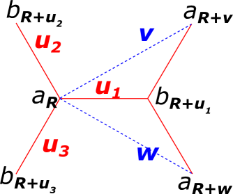
Figure 1: The honeycomb lattice, indicated in red, as bipartite lattice formed by two triangular sublattices generated by the vectors ${\bf v}$ and ${\bf w}$, indicated in blue and given in the main text. The displacement between the two sublattice is given by the links of the honeycomb lattice, ${\bf u_{j}}$, $j=1,2,3$, for instance of ${\bf u_{1}}$. The links add up to zero, $\sum_{j}{\bf u_{j}}=0$, and are chosen here to be of unit length. In terms of the generators they read, ${\bf u_{1}}=\frac{{\bf v}+{\bf w}}{3}$, ${\bf u_{2}}=\frac{{\bf v}-2{\bf w}}{3}$, and ${\bf u_{3}}=\frac{{\bf w}-2{\bf v}}{3}$.

The second step is to determine the shape of the lattice we are interested in, see Fig. 1. The honeycomb lattice where the links are

$${\bf u_{1}}=(1,0),\ \ \ \ \ {\bf u_{2}}=(-\frac{1}{2},\frac{\sqrt{3}}{2}),\ \ \ \ \ {\bf u_{3}}=(-\frac{1}{2},-\frac{\sqrt{3}}{2}),$$ (5)

is the superposition of two Bravis lattices generated by ${\bf v}={\bf u_{1}}-{\bf u_{3}}=(3/2,\sqrt{3}/2)$ and ${\bf w}={\bf u_{1}}-{\bf u_{2}}=(3/2,-\sqrt{3}/2)$ and displaced by ${\bf u_{1}}$ (or any other link vectors).

The third step is to substitute the derivatives of the spinor in $x$ and $y$ with finite differences of the spinor components’ on the lattice points, and to substitute the integral with a sum over the lattice points.

There are two issues. The first is that there are many equivalent ways of decomposing a displacement parallel to $x$ and $y$ in terms of the vectors ${\bf v}$ and ${\bf w}$ (${\bf u_{1}}$, ${\bf u_{2}}$, and ${\bf u_{3}}$), i.e., many collections of points can be chosen to compute the same derivative. The second is that the spinor components $a({\bf r})$ and $b({\bf r})$ do not live on the same site. This second problem is related to the first one as in first approximation for instance

$$b({\bf R})\simeq b({\bf R}+{\bf u_{1}})-\partial_{x}b({\bf R}+{\bf u_{1}}),$$ (6)

where ${\bf R}=m{\bf v}+n{\bf w}$, $m,n\in{\mathbb{Z}}$ is a generic point in the sublattice occupied by the fermion $a$.

One possible way of proceeding is to consider the following relations that are valid at first order

$$\partial_{x}a^{\dagger}({\bf R}) \simeq\frac{1}{3}\left(a^{\dagger}_{{\bf R}+{\bf v}}+a^{\dagger}_{{\bf R}+{\bf w}}-2a^{\dagger}_{\bf R}\right)$$ (7)

$$\partial_{y}a^{\dagger}({\bf R}) \simeq\frac{1}{\sqrt{3}}\left(a^{\dagger}_{{\bf R}+{\bf v}}-a^{\dagger}_{{\bf R}+{\bf w}}\right)$$ (8)

$$\partial_{x}b({\bf R}) \simeq\frac{1}{3}\left(2b_{{\bf R}+{\bf u_{1}}}-b_{{\bf R}+{\bf u_{2}}}-b_{{\bf R}+{\bf u_{3}}}\right)$$ (9)

$$\partial_{y}b({\bf R}) \simeq\frac{1}{\sqrt{3}}\left(b_{{\bf R}+{\bf u_{2}}}-b_{{\bf R}+{\bf u_{3}}}\right)$$ (10)

$$b({\bf R}) \simeq\frac{1}{3}\left(b_{{\bf R}+{\bf u_{1}}}+b_{{\bf R}+{\bf u_{2}}}+b_{{\bf R}+{\bf u_{3}}}\right)$$ (11)

$$\simeq\frac{1}{3}\left(-2b_{{\bf R}+{\bf v}+{\bf u_{1}}}+b_{{\bf R}+{\bf v}+{\bf u_{2}}}+4b_{{\bf R}+{\bf v}+{\bf u_{3}}}\right)$$ (12)

$$\simeq\frac{1}{3}\left(-2b_{{\bf R}+{\bf w}+{\bf u_{1}}}+4b_{{\bf R}+{\bf w}+{\bf u_{2}}}+b_{{\bf R}+{\bf w}+{\bf u_{3}}}\right)\,.$$ (13)

The expressions above can be derived by noticing that at first order, by indicating with $c$ generically $a$, $b$, $a^{\dagger}$, $b^{\dagger}$ and with ${\bf S}$ a generic vector, $c({\bf R}+{\bf S})\simeq c({\bf R})+{\bf S}\cdot{\bf\nabla}\,c({\bf R})$, which by linearity implies

$$\sum_{l}d_{l}\,c({\bf R}+{\bf S}_{l})=\left(\sum_{l}d_{l}\right)\,c({\bf R})+\left(\sum_{l}d_{l}{\bf S}_{l}\right)\cdot{\bf\nabla}\,c({\bf R}).$$ (14)

Thus, in order to obtain the expressions for the derivatives along $\hat{x}$ ($\hat{y}$), one has simply to require (or check in this case) that $\sum_{l}d_{l}=0$ and $\sum_{l}d_{l}{\bf S}_{l}=\hat{x}$ ($\hat{y}$). Instead, the expressions for $b({\bf R})$ are obtained by requiring that $\sum_{l}d_{l}=1$ and $\sum_{l}d_{l}{\bf S}_{l}=0$. As explained before the set of displacements $\{{\bf S}_{l}\}$ is chosen in order to construct the desired tightbinding model.

By using the relations (13) we can discretize the Hamiltonian (2). In particular, we notice that tricky binomials like $a({\bf R}+{\bf v})^{\dagger}b({\bf R})$ and $a({\bf R}+{\bf w})^{\dagger}b({\bf R})$ can be expressed in terms of nearest-neighbor tunnelings

$$a({\bf R}+{\bf v})^{\dagger}b({\bf R}) \rightarrow\frac{1}{3}a_{\bf R+{\bf v}}^{\dagger}\left(-2b_{{\bf R}+{\bf v}+{\bf u_{1}}}+b_{{\bf R}+{\bf v}+{\bf u_{2}}}+4b_{{\bf R}+{\bf v}+{\bf u_{3}}}\right)$$ (15)

$$a({\bf R}+{\bf w})^{\dagger}b({\bf R}) \rightarrow\frac{1}{3}a_{\bf R+{\bf w}}^{\dagger}\left(-2b_{{\bf R}+{\bf w}+{\bf u_{1}}}+4b_{{\bf R}+{\bf w}+{\bf u_{2}}}+b_{{\bf R}+{\bf w}+{\bf u_{3}}}\right).$$ (16)

By exploiting that the sum over ${\bf R}$ is running over the whole plane (which is a good approximation for a sufficiently large lattice) we can replace for instance $\sum_{\bf R}a_{{\bf R}+{\bf v}}^{\dagger}b_{{\bf R}+{\bf v}+{\bf u_{1}}}$ with $\sum_{\bf R}a_{{\bf R}}^{\dagger}b_{{\bf R}+{\bf u_{1}}}$ and get as lattice Hamiltonian

$$H=-i\sum_{\bf R}\sum_{j=1}^{3}J_{{\bf u_{j}},{\bf R}}a_{{\bf R}}^{\dagger}b_{{\bf R}+{\bf u_{j}}}+{\rm H.c.}\,,$$ (17)

where

$$J_{{\bf u_{1}},{\bf R}} =\frac{1}{9}\left[\left(J_{{\bf R}-{\bf v}}+J_{{\bf R}-{\bf w}}+4J_{{\bf R}}\right)+\sqrt{3}i\left(J_{{\bf R}-{\bf v}}-J_{{\bf R}-{\bf w}}\right)\right],$$ (18)

$$J_{{\bf u_{2}},{\bf R}} =-\frac{1}{18}\left[\left(J_{{\bf R}-{\bf v}}+4J_{{\bf R}-{\bf w}}+J_{{\bf R}}\right)-\sqrt{3}i\left(J_{{\bf R}-{\bf v}}-4J_{{\bf R}-{\bf w}}-3J_{{\bf R}}\right)\right],$$ (19)

$$J_{{\bf u_{3}},{\bf R}} =-\frac{1}{18}\left[\left(4J_{{\bf R}-{\bf v}}+J_{{\bf R}-{\bf w}}+J_{{\bf R}}\right)-\sqrt{3}i\left(4J_{{\bf R}-{\bf v}}-J_{{\bf R}-{\bf w}}+3J_{{\bf R}}\right)\right].$$ (20)

Notice that the global phase $-i$ can be eliminated, for instance, by a phase redefinition of the $a$’s, $i\,a_{\bf R}\to a_{\bf R}$, which obviously implies $-i\,a^{\dagger}_{\bf R}\to a^{\dagger}_{\bf R}$. As we constructed our lattice Hamiltonian to be graphene like, it is worth to consider the propagation in the Minkowski metric, i.e., for a spatially constant hopping, $J_{\bf R}=J$. The hopping over the different links reduce to

$$J_{\bf u_{1}}\rightarrow\frac{2}{3}J,\ \ \ \ J_{\bf u_{2}}\rightarrow\frac{2}{3}e^{-i\frac{2\pi}{3}}J,\ \ \ \ J_{\bf u_{3}}\rightarrow\frac{2}{3}e^{i\frac{2\pi}{3}}J.$$ (21)

At the first sight, the outcome is quite surprising as the hopping is not the same for the different links as in graphene and not even real. Furthermore, it is not possible to remove the phases by a global phase transformation of the spinor $\psi$, or equivalently by a redefinition of the Pauli matrices by a rotation around the $z$-axis. However, there is nothing wrong with the lattice Hamiltonian we have found. Indeed, as a check, we can verify the existence of two Dirac points, which are equivalent to the graphene-like model but have a different location in the Brillouin zone. For the hopping (21), the condition that Hamiltonian in momentum space is zero, $\sum_{j=1}^{3}J_{\bf u_{j}}e^{i{\bf k}\cdot{\bf u_{j}}}=0$, implies that as inequivalent Dirac points can be chosen the origin, ${\bf k}=(0,0)$ ($\sum_{j=1}^{3}J_{\bf u_{j}}=0$), and ${\bf k}=\frac{4\pi}{3\sqrt{3}}(\frac{1}{2},-\frac{\sqrt{3}}{2})$, which lays on the frontier of the Brillouin zone. Thus, this configuration corresponds to a displacement in momentum of the Brillouin zone of ${\bf K}_{D}=\frac{4\pi}{3\sqrt{3}}(0,1)$, which is equivalent to the following local gauge transformation in momentum space

$$a_{\bf R}\to e^{-i{\bf K}_{D}\cdot{\bf R}}a_{\bf R},$$ (22)

$$a^{\dagger}_{\bf R}\to e^{i{\bf K}_{D}\cdot{\bf R}}a^{\dagger}_{\bf R},$$ (23)

$$b_{\bf R}\to e^{-i{\bf K}_{D}\cdot{\bf R}}b_{\bf R},$$ (24)

$$b^{\dagger}_{\bf R}\to e^{i{\bf K}_{D}\cdot{\bf R}}b^{\dagger}_{\bf R},$$ (25)

The transform above implies for the tunnelings

$$J_{{\bf u_{j}},{\bf R}}\to e^{-i{\bf K}_{D}\cdot{\bf u_{j}}}J_{{\bf u_{j}},{\bf R}},$$ (26)

which gives the phases in (21) as ${\bf K}_{D}\cdot{\bf u_{1}}=0$, and ${\bf K}_{D}\cdot{\bf u_{2}}=-{\bf K}_{D}\cdot{\bf u_{3}}=\frac{2\pi}{3}$. Note that the module of the tunneling we have obtained for the Minkowski case, $\frac{2}{3}J$, it is nothing more than the relation between the tunneling and Fermi velocity in graphene that for the lattice spacing we have chosen is precisely equal to $J$. Coming back to a generic curved spacetime described by the metric (1), what we find suggests that our lattice model (17) is gauge equivalent to the gravitational deformation of graphene-like model. In the next section we will show how this relation can be made explicit by the inclusion of the gauge field coupling in the continuous Hamiltonian we start with.

3 Gauge&Gravity coupled Dirac Hamiltonian on a hexagonal lattice

I am going to repeat the same exercise as in the previous section for Dirac charged particles coupled to a gauge field and moving in the metric (1). Note that this exercise has some relation with the debate deJuan12 on whether the effect of ripples and other in graphene is better accounted by gravitational distortion or by the presence of gauge fields. For a comprehensive discussion we refer the reader to Arias15 where a unique relation between the space curvature and the magnetic field induced by ripples in graphene is established.

By the gauge choice $A_{0}=0$ , this is equivalent to consider the Hamiltonian

$$H=\frac{i}{2}\int{\rm dx}{\rm dy}J({\bf r})\left((\partial_{p}-iA_{p}({\bf r}))\psi^{\dagger}({\bf r})\sigma_{p}\psi({\bf r})-\psi^{\dagger}({\bf r})\sigma_{p}(\partial_{p}+iA_{p}({\bf r}))\psi({\bf r})\right)\,,$$ (27)

which in components reads

$$H=\frac{i}{2}\int{\rm dx}{\rm dy}J({\bf r})\left[(\partial_{x}-i\partial_{y}-i(A_{x}{\bf r})-iA_{y}{\bf r}))a^{\dagger}({\bf r})b({\bf r})\right.\cr\left.-a^{\dagger}({\bf r})(\partial_{x}-i\partial_{y}+i(A_{x}{\bf r})-iA_{y}{\bf r}))b({\bf r})\right]+{\rm H.c.}\,.$$ (28)

The only new ingredient that we have to add to the recipe is

$$\left(\partial_{x}-iA_{x}\right)a^{\dagger}({\bf R}) \simeq\frac{1}{3}\left(e^{-i\int_{\bf R}A_{v}}a^{\dagger}_{{\bf R}+{\bf v}}+e^{-i\int_{\bf R}A_{w}}a^{\dagger}_{{\bf R}+{\bf w}}-2a^{\dagger}_{\bf R}\right)$$ (29)

$$\left(\partial_{y}-iA_{y}\right)a^{\dagger}({\bf R}) \simeq\frac{1}{\sqrt{3}}\left(e^{-i\int_{\bf R}A_{v}}a^{\dagger}_{{\bf R}+{\bf v}}-e^{-i\int_{\bf R}A_{w}}a^{\dagger}_{{\bf R}+{\bf w}}\right)$$ (30)

$$\left(\partial_{x}+iA_{x}\right)b({\bf R}) \simeq\frac{1}{3}\left(2e^{i\int_{\bf R}A_{u_{1}}}b_{{\bf R}+{\bf u_{1}}}-e^{i\int_{\bf R}A_{u_{2}}}b_{{\bf R}+{\bf u_{2}}}-e^{i\int_{\bf R}A_{u_{3}}}b_{{\bf R}+{\bf u_{3}}}\right)$$ (31)

$$\left(\partial_{y}+iA_{y}\right)b({\bf R}) \simeq\frac{1}{\sqrt{3}}\left(e^{i\int_{\bf R}A_{u_{2}}}b_{{\bf R}+{\bf u_{2}}}-e^{i\int_{\bf R}A_{u_{3}}}b_{{\bf R}+{\bf u_{3}}}\right)\,,$$ (32)

where the expression $\int_{\bf R}A_{S}$ for a generic vector ${\bf S}$ is a short cut for the line integral $\int_{0}^{1}{\rm d}l\,{\bf S}\cdot{\bf A}({\bf R}+l\,{\bf S})$. Again the relations above can be checked by Taylor expanding the right hand sides at first order and by exploiting the linearity of the scalar products, ${\bf S}\cdot{\bf A}({\bf R})$.

By using the relation (13) and (32) we get again a Hamiltonian of the form (17) with the hopping of the form

$$J_{{\bf u_{1}},{\bf R}} =\frac{1}{9}\left[\left(J_{{\bf R}-{\bf v}}e^{-i\int_{{\bf R}-{\bf v}}A_{v}}+J_{{\bf R}-{\bf w}}e^{-i\int_{{\bf R}-{\bf w}}A_{w}}+J_{{\bf R}}\left(1+3e^{-i\int_{{\bf R}}A_{u_{1}}}\right)\right)\right.$$ (33)

$$\ \ \ \ \ \left.+\sqrt{3}i\left(J_{{\bf R}-{\bf v}}e^{-i\int_{{\bf R}-{\bf v}}A_{v}}-J_{{\bf R}-{\bf w}}e^{-i\int_{{\bf R}-{\bf w}}A_{w}}\right)\right],$$ (34)

$$J_{{\bf u_{2}},{\bf R}} =-\frac{1}{18}\left[\left(J_{{\bf R}-{\bf v}}e^{-i\int_{{\bf R}-{\bf v}}A_{v}}+4J_{{\bf R}-{\bf w}}e^{-i\int_{{\bf R}-{\bf w}}A_{w}}+J_{{\bf R}}\left(-2+3e^{-i\int_{{\bf R}}A_{u_{2}}}\right)\right)\right.$$ (35)

$$\ \ \ \ \ \left.-\sqrt{3}i\left(J_{{\bf R}-{\bf v}}e^{-i\int_{{\bf R}-{\bf v}}A_{v}}-4J_{{\bf R}-{\bf w}}e^{-i\int_{{\bf R}-{\bf w}}A_{w}}-3J_{{\bf R}}e^{-i\int_{{\bf R}}A_{u_{2}}}\right)\right],$$ (36)

$$J_{{\bf u_{3}},{\bf R}} =-\frac{1}{18}\left[\left(4J_{{\bf R}-{\bf v}}e^{-i\int_{{\bf R}-{\bf v}}A_{v}}+J_{{\bf R}-{\bf w}}e^{-i\int_{{\bf R}-{\bf w}}A_{w}}+J_{{\bf R}}\left(-2+3e^{-i\int_{{\bf R}}A_{u_{3}}}\right)\right)\right.$$ (37)

$$\ \ \ \ \ \left.-\sqrt{3}i\left(4J_{{\bf R}-{\bf v}}e^{-i\int_{{\bf R}-{\bf v}}A_{v}}-J_{{\bf R}-{\bf w}}e^{-i\int_{{\bf R}-{\bf w}}A_{w}}+3J_{{\bf R}}e^{-i\int_{{\bf R}}A_{u_{3}}}\right)\right].$$ (38)

As a final exercise we look for the pure gauge configuration that reproduces the graphene like Hamiltonian for $J_{\bf R}=J$. Under this condition the above expressions reduce to

$$J_{{\bf u_{1}},{\bf R}} =\frac{1}{9}\left[\left(e^{-i\int_{{\bf R}-{\bf v}}A_{v}}+e^{-i\int_{{\bf R}-{\bf w}}A_{w}}+\left(1+3e^{-i\int_{{\bf R}}A_{u_{1}}}\right)\right)\right.$$ (39)

$$\ \ \ \ \ \left.+\sqrt{3}i\left(e^{-i\int_{{\bf R}-{\bf v}}A_{v}}-e^{-i\int_{{\bf R}-{\bf w}}A_{w}}\right)\right]J,$$ (40)

$$J_{{\bf u_{2}},{\bf R}} =-\frac{1}{18}\left[\left(e^{-i\int_{{\bf R}-{\bf v}}A_{v}}+4e^{-i\int_{{\bf R}-{\bf w}}A_{w}}+\left(-2+3e^{-i\int_{{\bf R}}A_{u_{2}}}\right)\right)\right.$$ (41)

$$\ \ \ \ \ \left.-\sqrt{3}i\left(e^{-i\int_{{\bf R}-{\bf v}}A_{v}}-4e^{-i\int_{{\bf R}-{\bf w}}A_{w}}-3e^{-i\int_{{\bf R}}A_{u_{2}}}\right)\right]J,$$ (42)

$$J_{{\bf u_{3}},{\bf R}} =-\frac{1}{18}\left[\left(4e^{-i\int_{{\bf R}-{\bf v}}A_{v}}+e^{-i\int_{{\bf R}-{\bf w}}A_{w}}+\left(-2+3e^{-i\int_{{\bf R}}A_{u_{3}}}\right)\right)\right.$$ (43)

$$\ \ \ \ \ \left.-\sqrt{3}i\left(4e^{-i\int_{{\bf R}-{\bf v}}A_{v}}-e^{-i\int_{{\bf R}-{\bf w}}A_{w}}+3e^{-i\int_{{\bf R}}A_{u_{3}}}\right)\right]J$$ (44)

defining the Dirac lattice Hamiltonian on the honeycomb lattice for a generic magnetic background in flat space. It is easy to check that by taking ${\bf A}={\bf K}_{D}=\frac{4\pi}{3\sqrt{3}}(0,1)$ the tunnelings $J_{{\bf u_{j}},{\bf R}}$ become all equal and real as ${\bf K}_{D}\cdot{\bf v}=-{\bf K}_{D}\cdot{\bf w}={\bf K}_{D}\cdot{\bf u_{2}}=-{\bf K}_{D}\cdot{\bf u_{3}}=\frac{2\pi}{3}$ and ${\bf K}_{D}\cdot{\bf u_{1}}=0$. This can be regarded also as an non-trivial check of the validity of (38).

By choosing this pure gauge configuration, it follows that gravitational deformation of the graphene like Hamiltonian in a metric (1) is determined by the hopping

$$J_{{\bf u_{1}},{\bf R}} =\frac{1}{9}\left[\left(J_{{\bf R}-{\bf v}}+J_{{\bf R}-{\bf w}}+4J_{{\bf R}}\right)-\sqrt{3}i\left(J_{{\bf R}-{\bf v}}-J_{{\bf R}-{\bf w}}\right)\right],$$ (45)

$$J_{{\bf u_{2}},{\bf R}} =\frac{1}{9}\left[J_{{\bf R}-{\bf v}}+4J_{{\bf R}-{\bf w}}+J_{{\bf R}}\right],$$ (46)

$$J_{{\bf u_{3}},{\bf R}} =\frac{1}{9}\left[4J_{{\bf R}-{\bf v}}+J_{{\bf R}-{\bf w}}+J_{{\bf R}}\right].$$ (47)

4 Gravitational deformation of the graphene-like Hamiltonian for real and isotropic hopping

It is worth to notice the Minkowski metric is not the only one of the form (1) associated to an honeycomb tightbinding model with real and equal $J_{\bf u_{1}}=J_{\bf u_{2}}=J_{\bf u_{3}}=f(R)$ at each lattice site. In order to systematically analyze the problem, it is convenient to consider a more symmetric formulation for the hopping (47). As we can perform the completely equivalent derivation of the discrete Dirac Hamiltonian for ${\bf v},{\bf w}\to-{\bf v},-{\bf w}$, the left-right symmetry can be restored by mediating over the two expressions. Explicitly , we find

$$J_{{\bf u_{1}},{\bf R}} =\frac{1}{9}\left[\left(\langle J_{{\bf R}}\rangle_{\bf v}+\langle J_{{\bf R}}\rangle_{\bf w}+4J_{{\bf R}}\right)-\sqrt{3}i\left(\langle J_{{\bf R}}\rangle_{\bf v}-\langle J_{{\bf R}}\rangle_{\bf w}\right)\right],$$ (48)

$$J_{{\bf u_{2}},{\bf R}} =\frac{1}{9}\left[\langle J_{{\bf R}}\rangle_{\bf v}+4\langle J_{{\bf R}}\rangle_{\bf w}+J_{{\bf R}}\right],$$ (49)

$$J_{{\bf u_{3}},{\bf R}} =\frac{1}{9}\left[4\langle J_{{\bf R}}\rangle_{\bf v}+\langle J_{{\bf R}}\rangle_{\bf w}+J_{{\bf R}}\right].$$ (50)

where $\langle J_{{\bf R}}\rangle_{\bf v}\equiv 1/2(J_{{\bf R}+{\bf v}}+J_{{\bf R}-{\bf v}})$, and $\langle J_{{\bf R}}\rangle_{\bf w}\equiv 1/2(J_{{\bf R}+{\bf w}}+J_{{\bf R}-{\bf w}})$. It is immediate to realize that condition for the tunnelings to be real is

$$\langle J_{{\bf R}}\rangle_{\bf v}=\langle J_{{\bf R}}\rangle_{\bf w}.$$ (51)

If we further ask that

$$\langle J_{{\bf R}}\rangle_{\bf v}=\langle J_{{\bf R}}\rangle_{\bf w}=J_{\bf R},$$ (52)

then the tunnelings in the three directions become equal and proportional to the “local” Fermi velocity $J_{\bf R}$

$$J_{\bf u_{1}}=J_{\bf u_{2}}=J_{\bf u_{3}}=\frac{2}{3}J_{{\bf R}}.$$ (53)

Let me analyze the content of the conditions (51) and (52). Once restricted to smooth and slowly varying deformations of the Minkowski metric, the former, $\langle J_{{\bf R}}\rangle_{\bf v}=\langle J_{{\bf R}}\rangle_{\bf w}$ forces $\partial_{y}J(r)=0$, as periodic functions of about one lattice site’s period are ruled out by the previous assumption. The condition (52) implies linearity, hence $J({\bf r})$ has to be of the Rindler form with $J({\bf r})\propto(x-x_{0})$.

Thus, we conclude that whenever the metric can be written in the form (1) with a $J({\bf r})=J(x)$, the corresponding tightbinding Hamiltonian on the honeycomb lattice can be made real. Generically, the tunnelings will not be isotropic. The Dirac Hamiltonian in the Rindler spacetime (see Sect. 5.2) provides the only non-trivial instance of a honeycomb tightbinding model with real and isotropic tunnelings, but non constant Fermi velocity.

5 Curved spacetimes on brickwall lattices

I study now a deformed honeycomb lattice. In particular, I stick to the brickwall lattice that is especially simple and suitable for experiments Tarruell12 . The topological structure of the lattice is still the same: bipartite with coordination number equal to three. Formally, the Hamiltonian has the same expression as in the honeycomb

$$H=\sum_{\bf R}\sum_{j=1}^{3}J_{{\bf u_{j}},{\bf R}}\,b_{{\bf R}+{\bf u_{j}}}^{\dagger}a_{\bf R}+{\rm H.c.},$$ (54)

but this time the links are

$${\bf u_{1}}=(1+\Delta,0),\ \ \ {\bf u_{2}}=(\Delta,1),\ \ \ {\bf u_{3}}=(\Delta,-1),\ \ \ |\Delta|\leq 1,$$ (55)

which implies that the lattices for $a_{\bf R}$ and $b_{\bf R}$ are square with generators at $\pm\frac{\pi}{4}$ and the Brillouin zone has the same shape with $-(\pi-|k_{x}|)\leq k_{y}<\pi-|k_{x}|$ and $-\pi\leq k_{x}<\pi$.

Figure 2: The brickwall lattice, indicated in red, as bipartite lattice formed by two square sublattices, indicated in green and blue, respectively. The two sublattices are at $45^{\circ}$, have lattice spacing equal to $\sqrt{2}$, and are displaced horizontally one another. There are main cases: the displacement (to the right) is less ($\Delta>0$) than, equal ($\Delta=0$) to, or greater ($\Delta<0$) than 1, the length of the half diagonal of the square lattice. A peculiarity of the brickwall lattice is that not all the neighboring sites of the sublattices are connected. In this plot, the missing links are the horizontal ones to the right from the sublattice $a$ to the sublattice $b$. The allowed links, ${\bf u_{j}}$, $j=1,2,3$, are given in the main text in terms of $\Delta$.

5.1 Minkowski space

For constant hoppings $J_{{\bf u_{j}},{\bf R}}=J_{\bf u_{j}}$, the existence of Dirac points is easily shown by going in momentum space. Defining $a(b)_{\bf R}=\frac{1}{2\pi}\int_{BZ}e^{-i{\bf kR}}a(b)_{\bf k}$ we have

$$H =\int_{BZ}\sum_{j}J_{\bf u_{j}}e^{i{\bf ku_{j}}}b_{\bf k}^{\dagger}a_{\bf k}+{\rm H.c.}$$ (56)

$$=\int_{BZ}\psi_{\bf k}^{\dagger}\left\{\left[J_{\bf u_{1}}\cos((1+\Delta)k_{x})+(J_{\bf u_{2}}+J_{\bf u_{3}})\cos(\Delta k_{x})\cos(k_{y})\right.\right.$$ (57)

$$\hskip 56.9055pt\left.\left.-(J_{\bf u_{2}}-J_{\bf u_{3}})\sin(\Delta k_{x})\sin(k_{y})\right]\sigma_{x}\right.$$ (58)

$$\hskip 42.67912pt\left.+\left[J_{\bf u_{1}}\sin((1+\Delta)k_{x})+(J_{\bf u_{2}}+J_{\bf u_{3}})\sin(\Delta k_{x})\cos(k_{y})\right.\right.$$ (59)

$$\hskip 56.9055pt\left.\left.+(J_{\bf u_{2}}-J_{\bf u_{3}})\cos(\Delta k_{x})\sin(k_{y})\right]\sigma_{y}\right\}\psi_{\bf k},$$ (60)

where $\psi_{\bf k}\equiv\left(\begin{smallmatrix}a_{\bf k}\\ b_{\bf k}\end{smallmatrix}\right)$. The location of the Dirac in the BZ is determined by the solution of the system

$$J_{\bf u_{1}}\cos((1+\Delta)k_{x})+(J_{\bf u_{2}}+J_{\bf u_{3}})\cos(\Delta k_{x})\cos(k_{y})-(J_{\bf u_{2}}-J_{\bf u_{3}})\sin(\Delta k_{x})\sin(k_{y})=0$$

$$J_{\bf u_{1}}\sin((1+\Delta)k_{x})+(J_{\bf u_{2}}+J_{\bf u_{3}})\sin(\Delta k_{x})\cos(k_{y})+(J_{\bf u_{2}}-J_{\bf u_{3}})\cos(\Delta k_{x})\sin(k_{y})=0.$$

Let me specialize to the symmetric case $J_{\bf u_{j}}=J$ and $\Delta=0$. If follows that the two independent Dirac points are located at ${\bf K}_{\pm}=(0,\pm\frac{2\pi}{3})$. Note that, differently than in the graphene case, the Dirac points seat within the Brillouin zone, which is the square of vertices $(\pm\pi,0)$ and $(0,\pm\pi)$, and not on its borders. Different choices of $\Delta$ and $J_{\bf u_{j}}$’s lead to different locations of the Dirac points. For the simple case considered here, the effective Hamiltonian is $H_{\pm}=\mp\sqrt{3}p_{y}\sigma_{x}+p_{x}\sigma_{y}$ which is telling us that the cone is anisotropic, i.e., the Fermi velocity in the $y$-direction is $\sqrt{3}$ times the one in the $x$-direction. A isotropic cone for $\Delta=0$ is given for instance by the choice $J_{\bf u_{2}}=J_{\bf u_{3}}=\frac{1}{\sqrt{3}}J_{\bf u_{1}}$. In this case the Dirac points are at $(0,\pm\frac{5\pi}{6})$. An alternative option is $J_{\bf u_{2}}=J_{\bf u_{3}}=\frac{1}{\sqrt{2}}J_{\bf u_{1}}$: in this case the Dirac points are at the boundary of the Brillouin zone, e.g., $(\pi,0)$ and $(0,\pi)$. Note that the choice $J_{\bf u_{2}}=J_{\bf u_{3}}$ implies that the Dirac points lie on the $y$-axis, for any value of $\Delta$.

In fact we can get a isotropic cone by construction, i.e., by discretizing the isotropic Dirac Hamiltonian on a brick lattice. By setting the Fermi velocity to 1 and by discretizing on the $b$-sites, ${\bf r}=m({\bf u}_{1}+{\bf u}_{2})+n({\bf u}_{1}-{\bf u}_{2})=(m+n,m-n)$, one gets

$$H_{M}=\frac{1}{2}\sum_{\bf r}\left(i(\partial_{x}-i\partial_{y})a^{\dagger}_{\bf r}b_{\bf r}\right)+{\rm H.c.}\,,$$ (61)

where the discrete derivatives are

$$\partial_{x}a_{\bf r} =a_{{\bf r}+{\bf u}_{1}}-\frac{1}{2}(a_{{\bf r}+{\bf u}_{2}}+a_{{\bf r}-{\bf u}_{2}}),$$ (62)

$$\partial_{y}a_{\bf r} =\frac{1}{2}(a_{{\bf r}+{\bf u}_{2}}-a_{{\bf r}-{\bf u}_{2}}).$$ (63)

The substitution gives

$$H_{M}=\frac{1}{2}\sum_{\bf r}\left(\left(e^{i\frac{\pi}{2}}a^{\dagger}_{{\bf r}+{\bf u}_{1}}+\frac{e^{-i\frac{3}{4}\pi}a^{\dagger}_{{\bf r}+{\bf u}_{2}}+e^{-i\frac{\pi}{4}}a^{\dagger}_{{\bf r}+{\bf u}_{3}}}{\sqrt{2}}\right)b_{\bf r}\right)+{\rm H.c.},$$ (64)

which, up to the gauge transformation $c_{\bf s}\to e^{i\frac{\pi}{4}({\bf s}\cdot{\bf u}_{2}+2)}c_{\bf s}$ (or equivalently, $c_{(x,y)}\to e^{i\frac{\pi}{4}(y+2)}c_{(x,y)}$), where $c_{\bf s}$ are both $a_{\bf s}$ and $b_{\bf s}$, is equivalent to the Hamiltonian (60) for $\Delta=0$ and $J_{\bf u_{1}}=1=\sqrt{2}J_{\bf u_{2}}=\sqrt{2}J_{\bf u_{3}}$.

5.2 Rindler space

Now I repeat the above construction for the Dirac Hamiltonian in 2+1 Rindler spacetime. Rindler spacetime is Minkowski spacetime viewed by an accelerated observer Misner ; Wald ; Sachs . In special relativity, an observer moving with constant acceleration follows an hyperbolic trajectory. For a unitary acceleration in natural unit, (for convenience in the following we take the speed of light to be $c=1$) in the positive $x$-axis, the trajectory in the parametric form reads

$$\begin{cases}t=\xi\sinh\eta\\ x=\xi\cosh\eta\end{cases}.$$ (65)

The parameter $\eta$ plays the role of the co-moving time coordinate for this observer, and $\xi$ of the co-moving space coordinate. They are called Rindler coordinates, and are related to the Minkowski Cartesian ones by (65) (see Fig. 3). The accelerated observer is at rest in Rindler spacetime. Notice the similarity with polar coordinates, where $\xi$ plays the role of a radius and $\eta$ is an angle in hyperbolic geometry. The principle of equivalence states that physics seen by a non-inertial observer can be absorbed by a change in her metric. Indeed, in these coordinates, the Minkowski metric becomes

$$ds^{2}=-\xi^{2}d\eta^{2}+d\xi^{2}+dy^{2},$$ (66)

which is known as the Rindler metric. It is of the form of (1) (once we rename $\xi$ with $t$ and $\xi$ with $x$), with a function $J$ linear in $\xi$. Notice that the Rindler time direction corresponds to a symmetry of the metric, i.e., it constitutes a Killing vector which is inequivalent to the usual Minkowski time direction. In fact, it corresponds to a boost transformation. In the polar coordinates view, it is the generator of hyperbolic rotations. Another peculiarity of a relativistic constant acceleration, which is reflected by the hyperbolic geometry, is that the back of a rigid stick oriented along $x$ has to accelerate more than its front. In fact, a static observer in Rindler spacetime feels a proper acceleration that it is inversely proportional to $\xi$. The acceleration diverges at $\xi=0$ that corresponds to a singularity in the coordinate system, singularity that is signaled in the Rindler metric (66) by the vanishing of $d\eta^{2}$ coefficient. This is the hallmark of an event horizon. Thus, spacetime is separated into two parts which do not communicate: the two Rindler wedges, $\xi>0$ and $\xi<0$. The existence of an event horizon is at the heart of many intriguing phenomena like the Unruh effect and the appearance of the Hawking radiation from black holes. In fact, the Rindler metric describes the near-horizon limit of a Schwartzschild black hole.

[width=9cm]rindler_coord

Figure 3: Rindler coordinates on 1+1D Minkowski spacetime, $\eta$ (Rindler time) and $\xi$ (Rindler space). The Rindler wedge, delimited by dashed lines, is the domain of validity of the coordinate patch. The dashed lines represent the horizon, i.e., the loci of infinity acceleration. Constant $\eta$ lines (green) are spacelike, and constant $\xi$ lines (red) are timelike. For simplicity, we plot the trajectories only in the right wedge, $x>0$, as the ones for the wedge $x<0$ can be obtained by reflection around the $y$-axis.

By renaming the Rindler coordinates by $t$ and $x$, the continuous Rindler Hamiltonian in Rindler spacetime reads

$$H_{R}=\frac{1}{2}\sum_{\bf r}|{\bf r}\cdot{\bf u}_{1}|\left(i(\partial_{x}-i\partial_{y})a^{\dagger}_{\bf r}b_{\bf r}\right)+{\rm H.c.},$$ (67)

where the discrete derivatives are taken as in (63).

After the substitution we have

$$H_{R}=\frac{1}{2}\sum_{m,n}\left(\left(|m+n+\frac{1}{2}|\,e^{i\frac{\pi}{2}}a^{\dagger}_{m+n+1,m-n}\right.\right.\cr\left.\left.+\,|m+n|\,\frac{e^{-i\frac{3}{4}\pi}a^{\dagger}_{m+n,m-n+1}+e^{-i\frac{\pi}{4}}a^{\dagger}_{m+n,m-n-1}}{\sqrt{2}}\right)b_{m+n,m-n}\right)+{\rm H.c.},$$ (68)

where the value of the warp factor $|{\bf r}\cdot{\bf u}_{1}|$ is averaged over the corresponding link, such to give rise to anisotropy in the link intensity. The phases can be reabsorbed as in the Minkowski case and the Hamiltonian cast in a real form

$$H_{R}=\frac{1}{2}\sum_{m,n}\left(\left(|m+n+\frac{1}{2}|\,a^{\dagger}_{m+n+1,m-n}\right.\right.\cr\left.\left.+\,|m+n|\,\frac{a^{\dagger}_{m+n,m-n+1}+a^{\dagger}_{m+n,m-n-1}}{\sqrt{2}}\right)b_{m+n,m-n}\right)+{\rm H.c.}\,.$$ (69)

This is a possible choice for the implementation, up to an overall energy scale that fixes the “local” speed of light.

An alternative implementation can be obtained by “rotating the brick of $90^{\circ}$” (in fact it is a reflection) and defining ${\bf u}_{1}=(0,1)$, and ${\bf u}_{2}=-{\bf u}_{3}=(1,0)$. Accordingly, ${\bf r}=(m-n,m+n)$. Repeating the same exercise as before we have

$$H_{R}=\frac{1}{2}\sum_{\bf r}|{\bf r}\cdot{\bf u}_{2}|\left(i(\partial_{x}-i\partial_{y})a^{\dagger}_{\bf r}b_{\bf r}\right)+{\rm H.c.}\,,$$ (70)

where the discrete derivatives with respect to $x$ and $y$ are just exchanged

$$\partial_{x}a_{\bf r} =\frac{1}{2}(a_{{\bf r}+{\bf u}_{2}}-a_{{\bf r}-{\bf u}_{2}}),$$ (71)

$$\partial_{y}a_{\bf r} =a_{{\bf r}+{\bf u}_{1}}-\frac{1}{2}(a_{{\bf r}+{\bf u}_{2}}+a_{{\bf r}-{\bf u}_{2}}).$$ (72)

After the gauge transformation $c_{\bf s}\to e^{i\frac{\pi}{4}{\bf s}\cdot{\bf u}_{2}}c_{\bf s}$, the final Hamiltonian reads

$$H_{R}=\frac{1}{2}\sum_{m,n}\left(\left(\frac{|m-n+\frac{1}{2}|\,a^{\dagger}_{m-n+1,m+n}+|m-n-\frac{1}{2}|\,a^{\dagger}_{m-n-1,m+n}}{\sqrt{2}}\right.\right.\cr\left.\left.+\,|m+n|\,a^{\dagger}_{m-n,m+n+1}\right)b_{m-n,m+n}\right)+{\rm H.c.}\,.$$ (73)

5.3 Dirac Hamiltonian in Rindler space with extradimensions

The above Hamiltonians (69) and (73) can be conveniently implemented in a synthetic lattice. For synthetic lattice, I mean a lattice in which at least one of the spatial dimensions is obtained by promoting some internal degrees of freedom of the constituents –here the spin states for atoms– to sites of an extradimension Boada12 , also known as synthetic dimension Celi14 . The tunneling in the synthetic dimension is induced by some coherent coupling of the internal states. For atoms, such couplings can be induced by radiofrequency or by Raman pulses. The key advantage of synthetic lattices is that they are very versatile Rodriguez16 and convenient experimentally, as demonstrated in Stuhl15 ; Mancini15 , see also Celi15 .

As I am interested to have a synthetic lattice extended in the $x$-direction (perpendicular to the horizon), I implement the $y$-direction in the synthetic dimension by using atomic spin states. I indicate the spin states with an index $\sigma$ and the position along the chain with an index $l$. Note that on the sites occupied by the $b$-fermions, even (odd) values of $l$ correspond to even (odd) values of the spin $\sigma$, while for the $a$-sites exactly the opposite occurs, even (odd) $l$ correspond to odd (even) $\sigma$. Thus, by summing over all $l=-L,\dots,L$, I can use just one species with $S$ internal states. In case of (69), we have

$$H_{R}=\frac{1}{2}\sum_{l,\sigma}\left(\left(\sqrt{2}\,|l|\,(1-\frac{\delta_{\sigma,1}+\delta_{\sigma,S-1}}{2})c^{\dagger(\sigma+1)}_{l}\,+\,|l+\frac{\epsilon(l,\sigma)}{2}|\,c^{\dagger(\sigma)}_{l+\epsilon(l,\sigma)}\right)c^{\sigma}_{l}\right)+{\rm H.c.}\,,$$ (74)

where we have defined $\epsilon(l,\sigma)\equiv(-1)^{l+\sigma}$. Note that due to the definition of the discrete derivative in the $y$-direction, Eq. (63), the tunneling terms along $y$ have on the boundary of the synthetic dimension half of the strength than in the bulk. Such result is directly obtained from the Hamiltonian (69) by collecting in a unique “forward” tunneling terms in $y$ the forward and back tunneling terms in (69).

In case of (73), which is probably the easiest to be simulated, we have

$$H_{R}=\frac{1}{2}\sum_{l,\sigma}\left(\left(\sqrt{2}\,|l+\frac{1}{2}|\,(1-\frac{\delta_{l,-L}+\delta_{l,L-2}}{2})c^{\dagger(\sigma)}_{l+1}\,+\,|l|\,c^{\dagger(\sigma+\epsilon(l,\sigma))}_{l}\right)c^{\sigma}_{l}\right)+{\rm H.c.}\,.$$ (75)

A similar reasoning as above (with the interchange of $y$ with $x$) explains the boundary terms, this time in the real dimension.

It is worth to notice that the Hamiltonian (75) once specialized to a one-dimensional chain describes correctly the tightbinding Dirac Hamiltonian in 1D. As the

$$H_{R-1D}=\frac{1}{2}\sum_{\bf r}|{\bf r}\cdot{\bf u}_{1}|\left(i\partial_{x}a^{\dagger}_{\bf r}b_{\bf r}\right)+{\rm H.c.},$$

the final expression, a part a factor $\sqrt{2}$ will correspond to (75) for S=1, i.e.

$$H_{R-1D}=\frac{1}{2}\sum_{l}\left(|l+\frac{1}{2}|\,(1-\frac{\delta_{l,-L}+\delta_{l,L-2}}{2})c^{\dagger}_{l+1}\,c_{l}\right)+{\rm H.c.}\,.$$ (76)

6 $\pi$-flux Hamiltonian

The most elegant way of deriving the Dirac Hamiltonian in the $\pi$-flux form is to begin with a bipartite square lattice. As usual I start from (61). I take ${\bf u}_{1}=(1,0)$ and ${\bf u}_{2}=(0,1)$. Then, the fact that I want links turned on in any direction is telling me that all the neighbors $a_{{\bf r}+{\bf u}_{1}},a_{{\bf r}+{\bf u}_{2}},a_{{\bf r}-{\bf u}_{1}},a_{{\bf r}-{\bf u}_{2}}$ of $b_{\bf r}$ have to enter in the discrete derivative of $a_{\bf r}$. A simple choice is

$$\partial_{x}a_{\bf r} =\frac{a_{{\bf r}+{\bf u}_{1}}-a_{{\bf r}-{\bf u}_{1}}}{2},$$ (77)

$$\partial_{y}a_{\bf r} =\frac{a_{{\bf r}+{\bf u}_{2}}-a_{{\bf r}-{\bf u}_{2}}}{2}.$$ (78)

After substituting the discrete derivatives we get

$$H_{M}=\frac{1}{4}\sum_{\bf r}\left(\left(e^{i\frac{\pi}{2}}a^{\dagger}_{{\bf r}+{\bf u}_{1}}+e^{-i\frac{\pi}{2}}a^{\dagger}_{{\bf r}-{\bf u}_{1}}+a^{\dagger}_{{\bf r}+{\bf u}_{2}}-a^{\dagger}_{{\bf r}-{\bf u}_{2}}\right)b_{\bf r}\right)+{\rm H.c.},$$ (79)

which, by applying the gauge transformation $c_{\bf s}\to e^{i\frac{\pi}{2}{\bf s}\cdot{\bf u}_{1}}c_{\bf s}$, is equivalent to

$$H_{M}=\frac{1}{4}\sum_{\bf r}\left(\left(a^{\dagger}_{{\bf r}+{\bf u}_{1}}+a^{\dagger}_{{\bf r}-{\bf u}_{1}}+a^{\dagger}_{{\bf r}+{\bf u}_{2}}-a^{\dagger}_{{\bf r}-{\bf u}_{2}}\right)b_{\bf r}\right)+{\rm H.c.}\,.$$ (80)

By using just a single species the above Hamiltonian can be cast in the more familiar form

$$H_{\text{M $\pi$-flux}}=\frac{1}{2}\sum_{m,n}\left(\left(c^{\dagger}_{m+1,n}+(-1)^{m+n}c^{\dagger}_{m,n+1}\right)c_{m,n}\right)+{\rm H.c.}\,.$$ (81)

The step to Rindler Hamiltonian is extremely easy: we have to include the dependence of hopping strength on the distance from the horizon, for instance, measured from the center of the link. By placing the horizon at $m=0$ we have

$$H_{\text{R $\pi$-flux}}=\frac{1}{2}\sum_{m,n}\left(\left(|m+\frac{1}{2}|\,\,c^{\dagger}_{m+1,n}+(-1)^{m+n}|m|\,c^{\dagger}_{m,n+1}\right)c_{m,n}\right)+{\rm H.c.}\,.$$ (82)

It is worth to note that it is immediate to promote the position index $n$ to a spin label and to implement the direction parallel to the horizon as a synthetic dimension. Let me just comment that in order to simulate the Unruh effect we proposed in Rodriguez16 to implement a similar Hamiltonian to the one above, but with the $\pi$ flux realized in the symmetric gauge, as it is easier to achieve in optically shaken in 2D real lattices (cf. Aidelsburger.13 ; Miyake.13 ; Kennedy.15 ).

7 Conclusions & Outlook

In this paper, I have illustrated the power of our top-down approach: formulating the Dirac Hamiltonian in curved spacetime directly in position space allows for the construction of several models of emerging gravitating Dirac fermions that can be simulated in optical lattices. It is worth to notice that this approach is in principle useful in any dimensions, and it could be extended to time-dependent metrics. Furthermore, as top-down approach allows the choice of the lattice and, thus, of its properties under parity symmetry, it can be used for obtained lattice formulation of topological insulators in specific classes in generic dimension as we do in Bikash for 3D models.

Here I have considered naive Dirac Hamiltonian as doubling does not play a major role, for instance, in the Unruh effect. Obviously, doubling could be avoided, for instance, by including generalization of Wilson or domain wall fermions Rubakov83 ; Callan85 to curved spacetime. Such research direction may be interesting both for testing which properties of known topological models are altered by coupling to gravity (cf. Can14 ), or for considering interacting gravitating fermions. The former direction requires the introduction of “mass” terms that are compatible with the Dirac Hamiltonian in curved spacetimes and can open a gap, as it happens in Minkowski spacetime. Such terms are not discussed here but they can be simply achieved by making the ordinary mass terms in Minkowski spacetimes, e.g, the staggered chemical potential for the $\pi$-flux formulation of the tightbinding Dirac Hamiltonian, position dependent. For the optical metrics of Eq. (1), such dependence is determined by the local Fermi velocity $J({\bf r})$, as it happens for the tunneling terms.

The possibility of considering strongly interacting gravitating matter, and perhaps the possibility of including matter backreaction on the artificial metric via density-dependent hopping Dutta15 are very appealing. They are unique and distinctive features of our quantum simulation strategy based on ultracold fermionic atoms in optical lattices developed in Boada2010b and Rodriguez16 , and applied here, features that distinguish it from other analogue gravity approaches.

- (1) "The Nobel Prize in Physics 2010". Nobelprize.org. Nobel Media AB 2014. Web. 30 Nov 2016. <http://www.nobelprize.org/nobel_prizes/physics/laureates/2010/>
- (2) "The Nobel Prize in Physics 2016". Nobelprize.org. Nobel Media AB 2014. Web. 30 Nov 2016. <http://www.nobelprize.org/nobel_prizes/physics/laureates/2016/>
- (3) C. L. Kane and E. J. Mele, “Z 2 topological order and the quantum spin hall effect,” Phys. Rev. Lett., vol. 95, p. 146802, 2005.
- (4) F. Guinea, N. M. R. Peres, K. S. Novoselov, A. K. Geim, and A. C. Neto, “The electronic properties of graphene,” Rev. Mod. Phys., vol. 81, p. 109, 2009.
- (5) P. R. Wallace, “The band theory of graphite,” Phys. Rev., vol. 71, p. 622, 1947.
- (6) A. P. Schnyder, S. Ryu, A. Furusaki, and A. W. Ludwig, “Classification of topological insulators and superconductors in three spatial dimensions,” Phys. Rev. B, vol. 78, p. 195125, 2008.
- (7) M. Z. Hasan and C. L. Kane, “Colloquium: topological insulators,” Rev. Mod. Phys., vol. 82, p. 3045, 2010.
- (8) S. Y. Xu, C. Liu, S. K. Kushwaha, R. Sankar, J. W. Krizan, I. Belopolski, M. Neupane, G. Bian, N. Alidoust, T. R. Chang, and H. T. Jeng, “Observation of fermi arc surface states in a topological metal,” Science, vol. 347, no. 6219, pp. 294–298, 2015.
- (9) C. K. Chiu, J. C. Teo, A. P. Schnyder, and S. Ryu, “Classification of topological quantum matter with symmetries,” Rev. Mod. Phys., vol. 88, p. 035005, 2016.
- (10) T. Salger, C. Grossert, S. Kling, and M. Weitz Phys. Rev. Lett., vol. 107, p. 240401, 2011.
- (11) P. Soltan-Panahi, “et al,” Nat. Phys, vol. 7, p. 434, 2011.
- (12) L. Duca, T. Li, M. Reitter, I. Bloch, M. Schleier-Smith, and U. Schneider Science, vol. 347, p. 288, 2015.
- (13) L. Tarruell, D. Greif, T. Uehlinger, G. Jotzu, and T. Esslinger Nature, vol. 483, p. 302, 2012.
- (14) M. Polini, F. Guinea, M. Lewenstein, H. C. Manoharan, and V. Pellegrini Nat. Nanotechnol, vol. 8, p. 625, 2013.
- (15) T. Jacqmin, I. Carusotto, I. Sagnes, M. Abbarchi, D. D. Solnyshkov, G. Malpuech, E. Galopin, A. Lemaître, J. Bloch, and A. Amo Phys. Rev. Lett, vol. 112, p. 116402, 2014.
- (16) G. Juzeliunas, J. Ruseckas, M. Lindberg, L. Santos, and P. Öhberg, “Quasirelativistic behavior of cold atoms in light fields,” Phys. Rev. A, vol. 77, p. 011802, 2008.
- (17) R. G. Unanyan, J. Otterbach, M. Fleischhauer, J. Ruseckas, V. Kudriaŝov, and G. Juzeliunas, “Spinor slow-light and dirac particles with variable mass,” Phys. Rev. Lett., vol. 105, p. 173603, 2010.
- (18) Y. J. Lin, K. Jiménez-García, and I. B. Spielman, “Spin-orbit-coupled bose-einstein condensates,” Nature, vol. 471, no. 7336, pp. 83–86, 2011.
- (19) V. Galitski and I. B. Spielman, “Spin-orbit coupling in quantum gases,” Nature, vol. 494, no. 7435, pp. 49–54, 2013.
- (20) L. Huang, Z. Meng, P. Wang, P. Peng, S. L. Zhang, L. Chen, D. Li, Q. Zhou, and J. Zhang, “Experimental realization of two-dimensional synthetic spin-orbit coupling in ultracold fermi gases,” Nature Physics, vol. 12, no. 6, pp. 540–544, 2016.
- (21) T. Uehlinger, D. Greif, G. Jotzu, L. Tarruell, T. Esslinger, L. Wang, and M. Troyer, “Double transfer through dirac points in a tunable honeycomb optical lattice,” The European Physical Journal Special Topics, vol. 217, no. 1, pp. 121–133, 2013.
- (22) M. Lewenstein, A. Sanpera, and V. Ahufinger, Ultracold atoms in optical lattices. Oxford University Press, 2012.
- (23) A. Celi, A. Sanpera, V. Ahufinger, and M. Lewenstein, “Quantum optics and frontiers of physics: The third quantum revolution,” Physica Scripta, vol. 92, no. 1, 2016.
- (24) L. Mazza, A. Bermudez, N. Goldman, M. Rizzi, M. A. Martin-Delgado, and M. Lewenstein, “An optical-lattice-based quantum simulator for relativistic field theories and topological insulators,” New Journal of Physics, vol. 14, p. 015007, 2012.
- (25) F. D. M. Haldane, “Model for a quantum hall effect without landau levels: Condensed-matter realization of the" parity anomaly",” Phys. Rev. Letters, vol. 61, p. 2015, 1988.
- (26) G. Jotzu, M. Messer, R. Desbuquois, M. Lebrat, T. Uehlinger, D. Greif, and T. Esslinger, “Experimental realization of the topological haldane model with ultracold fermions,” Nature, vol. 515, no. 7526, pp. 237–240, 2014.
- (27) H. B. Nielsen and M. Ninomiya, “A no-go theorem for regularizing chiral fermions,” Physics Letters B, vol. 105, no. 2, pp. 219–223, 1981.
- (28) K. S. et al.. Novoselov Nature, vol. 438, p. 197, 2005.
- (29) Y. Zhang, Y. W. Tan, H. L. Stormer, and P. Kim Nature, vol. 438, p. 201, 2005.
- (30) A. K. Geim and K. S. Novoselov Nature Materials, vol. 6, p. 183, 2007.
- (31) N. Goldman, A. Kubasiak, A. Bermudez, P. Gaspard, M. Lewenstein, and M. A. Martin-Delgado, “Non-abelian optical lattices: Anomalous quantum hall effect and dirac fermions,” Phys. Rev. Lett., vol. 103, p. 035301, 2009.
- (32) H. Watanabe, Y. Hatsugai, and H. Aoki, “Half-integer contributions to the quantum hall conductivity from single dirac cones,” Phys. Rev. B, vol. 82, p. 241403, 2010.
- (33) O. Klein Z. Phys., vol. 53, p. 157, 1929.
- (34) E. Schrödinger Sitz. Preuss. Akad. Wiss. Phys. Math. Kl., vol. 24, p. 418, 1930.
- (35) G. David and J. Cserti, “General theory of zitterbewegung,” Phys. Rev. B, vol. 81, p. 121417, 2010.
- (36) J. Cserti and G. Dávid Phys. Rev. B, vol. 74, p. 172305, 2006.
- (37) T. M. Rusin and W. Zawadzki Phys. Rev. B, vol. 80, p. 045416, 2009.
- (38) M. I. Katsnelson, N. K. S, and G. A. K Nature Physics, vol. 2, p. 620, 2006.
- (39) W. Zawadzki and T. M. Rusin J. Phys. Condens. Matter, vol. 23, p. 143201, 2011.
- (40) J. Otterbach, R. G. Unanyan, and M. Fleischhauer, “Confining stationary light: Dirac dynamics and klein tunneling,” Phys. Rev. Lett., vol. 102, p. 063602, 2009.
- (41) J. Y. Vaishnav and C. W. Clark Phys. Rev. Lett., vol. 100, p. 153002, 2008.
- (42) M. Merkl, F. E. Zimmer, G. Juzeliunas, and P. Öhberg Europhys. Lett., vol. 83, p. 54002, 2008.
- (43) Q. Zhang, J. Gong, and C. H. Oh Phys. Rev. A, vol. 81, p. 023608, 2010.
- (44) L. Lepori, G. Mussardo, and A. Trombettoni, “(3+1) massive dirac fermions with ultracold atoms in frustrated cubic optical lattices,” EPL (Europhysics Letters), vol. 92, p. 50003, 2010.
- (45) L. J. LeBlanc, M. C. Beeler, K. Jiménez-García, A. R. Perry, S. Sugawa, R. A. Williams, and I. B. Spielman, “Direct observation of zitterbewegung in a bose-einstein condensate,” New Journal of Physics, vol. 15, p. 073011, 2013.
- (46) J. Casanova, J. J. García-Ripoll, R. Gerritsma, C. F. Roos, and E. Solano Phys. Rev. A, vol. 82, p. 020101, 2010.
- (47) R. Gerritsma, B. P. Lanyon, G. Kirchmair, F. Zähringer, C. Hempel, J. Casanova, J. J. García-Ripoll, E. Solano, R. Blatt, and C. F. Roos Phys. Rev. Lett., vol. 106, p. 060503, 2011.
- (48) L. Lamata, J. León, T. Schätz, and E. Solano Phys. Rev. Lett., vol. 98, p. 253005, 2007.
- (49) R. Gerritsma, G. Kirchmair, F. Zähringer, E. Solano, R. Blatt, and C. F. Roos Nature, vol. 463, p. 68, 2010.
- (50) J. Casanova, C. Sabín, J. León, I. L. Egusquiza, R. Gerritsma, C. F. Roos, J. J. García-Ripoll, and E. Solano, “Quantum simulation of the majorana equation and unphysical operations,” Phys. Rev. X, vol. 1, p. 021018, 2011.
- (51) S. Longhi Opt. Lett., vol. 35, p. 235, 2010.
- (52) S. Longhi J. Phys. B: At. Mol. Opt. Phys., vol. 43, p. 205402, 2010.
- (53) F. Dreisow, M. Heinrich, R. Keil, A. Tünnermann, S. Nolte, S. Longhi, and A. Szameit Phys. Rev. Lett., vol. 105, p. 143902, 2010.
- (54) J. Schliemann, D. Loss, and R. M. Westervelt Phys. Rev. Lett., vol. 94, p. 206801, 2005.
- (55) J. S. Pedernales, R. Di Candia, D. Ballester, and E. Solano, “Quantum simulations of relativistic quantum physics in circuit qed,” New Journal of Physics, vol. 15, p. 055008, 2013.
- (56) S. Liu, C. J. Shan, Z. M. Zhang, and Z. Y. Xue, “Simulation of the majorana equation in circuit qed,” Quantum Information Processing, vol. 13, no. 8, pp. 1813–1823, 2014.
- (57) Z. Lan, A. Celi, W. Lu, P. Öhberg, and M. Lewenstein, “Tunable multiple layered dirac cones in optical lattices,” Phys. Rev. Lett., vol. 107, p. 253001, 2011.
- (58) C. Noh, B. M. Rodriguez-Lara, and D. G. Angelakis, “Quantum simulation of neutrino oscillations with trapped ions,” New Journal of Physics, vol. 14, p. 033028, 2012.
- (59) Z. S. Wang, X. Cai, and H. Pan, “Trapped ionic simulation of neutrino electromagnetic properties in neutrino oscillation,” Nuclear Physics B, vol. 900, pp. 560–575, 2015.
- (60) A. Bermudez, L. Mazza, M. Rizzi, N. Goldman, M. Lewenstein, and M. A. Martin-Delgado Phys. Rev. Lett., vol. 105, p. 190404, 2010.
- (61) N. Szpak and R. Schützhold, “Quantum simulator for the schwinger effect with atoms in bichromatic optical lattices,” Phys. Rev. A, vol. 84, p. 050101, 2011.
- (62) J. I. Cirac, P. Maraner, and J. K. Pachos, “Cold atom simulation of interacting relativistic quantum field theories,” Phys. Rev. Lett., vol. 105, p. 190403, 2010.
- (63) J. Casanova, L. Lamata, I. L. Egusquiza, R. Gerritsma, C. F. Roos, J. J. García-Ripoll, and E. Solano, “Quantum simulation of quantum field theories in trapped ions,” Phys. Rev. Lett., vol. 107, p. 260501, 2011.
- (64) F. L. Semião and M. Paternostro, “Quantum circuits for spin and flavor degrees of freedom of quarks forming nucleons,” Quantum Information Processing, vol. 11, pp. 67–75, 2012.
- (65) S. P. Jordan, K. S. Lee, and J. Preskill, “Quantum algorithms for quantum field theories,” Science, vol. 336, no. 6085, pp. 1130–1133, 2012.
- (66) H. P. Büchler, M. Hermele, S. D. Huber, M. P. Fisher, and P. Zoller, “Atomic quantum simulator for lattice gauge theories and ring exchange models,” Phys. Rev. Lett., vol. 95, p. 040402, 2005.
- (67) E. Zohar and B. Reznik, “Confinement and lattice quantum-electrodynamic electric flux tubes simulated with ultracold atoms,” Phys. Rev. Lett., vol. 107, p. 275301, 2011.
- (68) E. Zohar, J. I. Cirac, and B. Reznik, “Simulating compact quantum electrodynamics with ultracold atoms: Probing confinement and nonperturbative effects,” Phys. Rev. Lett., vol. 109, p. 125302, 2012.
- (69) L. Tagliacozzo, A. Celi, A. Zamora, and M. Lewenstein, “Optical abelian lattice gauge theories,” Annals of Physics, vol. 330, pp. 160–191, 2013.
- (70) D. Banerjee, M. Dalmonte, M. Müller, E. Rico, P. Stebler, U. J. Wiese, and P. Zoller, “Atomic quantum simulation of dynamical gauge fields coupled to fermionic matter: from string breaking to evolution after a quench,” Phys. Rev. Lett., vol. 109, p. 175302, 2012.
- (71) L. Tagliacozzo, A. Celi, P. Orland, M. W. Mitchell, and M. Lewenstein, “Simulation of non-abelian gauge theories with optical lattices,” Nature communications, vol. 4, 2013.
- (72) D. Banerjee, M. Bögli, M. Dalmonte, E. Rico, P. Stebler, U. J. Wiese, and P. Zoller, “Atomic quantum simulation of u (n) and su (n) non-abelian lattice gauge theories,” Phys. Rev. Lett., vol. 110, p. 125303, 2013.
- (73) E. Zohar, J. I. Cirac, and B. Reznik, “Cold-atom quantum simulator for su (2) yang-mills lattice gauge theory,” Phys. Rev. Lett., vol. 110, p. 125304, 2013.
- (74) K. Stannigel, P. Hauke, D. Marcos, M. Hafezi, S. Diehl, M. Dalmonte, and P. Zoller, “Constrained dynamics via the zeno effect in quantum simulation: Implementing non-abelian lattice gauge theories with cold atoms,” Phys. Rev. Lett., vol. 112, p. 120406, 2014.
- (75) V. Kasper, F. Hebenstreit, M. Oberthaler, and J. Berges, “Schwinger pair production with ultracold atoms,” Physics Letters B, vol. 760, pp. 742–746, 2016.
- (76) O. Dutta, L. Tagliacozzo, M. Lewenstein, and J. Zakrzewski, “Toolbox for abelian lattice gauge theories with synthetic matter.” preprint arXiv:1601.03303, 2016.
- (77) P. Hauke, D. Marcos, M. Dalmonte, and P. Zoller, “Quantum simulation of a lattice schwinger model in a chain of trapped ions,” Phys. Rev. X, vol. 3, p. 041018, 2013.
- (78) E. A. Martinez, C. A. Muschik, P. Schindler, D. Nigg, A. Erhard, M. Heyl, P. Hauke, M. Dalmonte, T. Monz, P. Zoller, and R. Blatt, “Real-time dynamics of lattice gauge theories with a few-qubit quantum computer,” Nature, vol. 534, pp. 516–519, 2016.
- (79) D. Yang, G. S. Giri, M. Johanning, C. Wunderlich, P. Zoller, and P. Hauke, “Analog quantum simulation of (1+ 1) d lattice qed with trapped ions.” preprint arXiv:1604.03124, 2016.
- (80) D. Marcos, P. Rabl, E. Rico, and P. Zoller, “Superconducting circuits for quantum simulation of dynamical gauge fields,” Phys. Rev. letters, vol. 111, p. 110504, 2013.
- (81) U. J. Wiese, “Ultracold quantum gases and lattice systems: quantum simulation of lattice gauge theories,” Annalen der Physik, vol. 525, no. 10-11, pp. 777–796, 2013.
- (82) E. Zohar, J. I. Cirac, and B. Reznik, “Quantum simulations of lattice gauge theories using ultracold atoms in optical lattices,” Reports on Progress in Physics, vol. 79, p. 014401, 2015.
- (83) L. Tagliacozzo and G. Vidal, “Entanglement renormalization and gauge symmetry,” Phys. Rev. B, vol. 83, p. 115127, 2011.
- (84) M. C. Bañuls, K. Cichy, K. Jansen, and J. I. Cirac, “The mass spectrum of the schwinger model with matrix product states,” High Energ. Phys., vol. 158, 2013.
- (85) Y. Liu, Y. Meurice, M. P. Qin, J. Unmuth-Yockey, T. Xiang, Z. Y. Xie, J. F. Yu, and H. Zou, “Exact blocking formulas for spin and gauge models,” Phys. Rev. D, vol. 88, p. 056005, 2013.
- (86) B. Buyens, J. Haegeman, K. Van Acoleyen, H. Verschelde, and F. Verstraete, “Matrix product states for gauge field theories,” Phys. Rev. letters, vol. 113, p. 091601, 2014.
- (87) L. Tagliacozzo, A. Celi, and M. Lewenstein, “Tensor networks for lattice gauge theories with continuous groups,” Phys. Rev. X, vol. 4, p. 041024, 2014.
- (88) P. Silvi, E. Rico, T. Calarco, and S. Montangero, “Lattice gauge tensor networks,” New Journal of Physics, vol. 16, p. 103015, 2014.
- (89) S. Kühn, J. I. Cirac, and M. Bañuls, “Quantum simulation of the schwinger model: A study of feasibility,” Phys. Rev. A, vol. 90, p. 042305, 2014.
- (90) J. Haegeman, K. Van Acoleyen, N. Schuch, J. I. Cirac, and F. Verstraete, “Gauging quantum states: from global to local symmetries in many-body systems,” Phys. Rev. X, vol. 5, p. 011024, 2015.
- (91) M. C. Bañuls, K. Cichy, J. I. Cirac, K. Jansen, and H. Saito, “Thermal evolution of the schwinger model with matrix product operators,” Phys. Rev. D, vol. 92, p. 034519, 2015.
- (92) S. Kühn, E. Zohar, J. I. Cirac, , and M. Bañuls, “Non-abelian string breaking phenomena with matrix product states,” J. High Energ. Phys., vol. 130, 2015.
- (93) E. Zohar, M. Burrello, T. B. Wahl, and J. I. Cirac, “Fermionic projected entangled pair states and local u(1) gauge theories,” Annals of Physics, vol. 363, pp. 385–439, 2015.
- (94) T. Pichler, M. Dalmonte, E. Rico, P. Zoller, and S. Montangero, “Real-time dynamics in u (1) lattice gauge theories with tensor networks,” Phys. Rev. X, vol. 6, p. 011023, 2016.
- (95) E. Zohar and M. Burrello, “Building projected entangled pair states with a local gauge symmetry,” New Journal of Physics, vol. 18, no. 4, p. 043008, 2016.
- (96) B. Dittrich, S. Mizera, and S. Steinhaus, “Decorated tensor network renormalization for lattice gauge theories and spin foam models,” New Journal of Physics, vol. 18, p. 053009, 2016.
- (97) E. Zohar, T. B. Wahl, M. Burrello, and J. I. Cirac, “Projected entangled pair states with non-abelian gauge symmetries: an su (2) study,” Annals of Physics, vol. 374, pp. 84–137, 2016.
- (98) P. Silvi, E. Rico, M. Dalmonte, F. Tschirsich, and S. Montangero, “Finite-density phase diagram of a (1+ 1)-d non-abelian lattice gauge theory with tensor networks.” preprint arXiv:1606.05510, 2016.
- (99) N. Birrell and P. Davies, Quantum fields in curved space. Cambridge University Press, 1982.
- (100) S. W. Hawking Comm. Math. Phys., vol. 43, p. 199, 1975.
- (101) W. G. Unruh Phys. Rev. D, vol. 14, p. 870, 1976.
- (102) C. Barceló, S. Liberati, and M. Visser Living Rev. Relativity, vol. 8, p. 12, 2005.
- (103) G. Volovik, The universe in a helium droplet. Oxford University Press, 2003.
- (104) G. W. Gibbons, “Some links between general relativity and other parts of physics,” in General Relativity, Cosmology and Astrophysics . International Publishing, pp. 91–110, 2014.
- (105) L. J. Garay, J. I. Anglin, J. R. Cirac, and Z. P. Phys. Rev. Lett., vol. 85, p. 4643, 2000.
- (106) P. O. Fedichev and U. R. Fischer Phys. Rev. Lett., vol. 91, p. 240407, 2003.
- (107) P. O. Fedichev and U. R. Fischer Phys. Rev. D, vol. 69, p. 064021, 2004.
- (108) P. O. Fedichev and U. R. Fischer Phys. Rev. A, vol. 69, p. 033602, 2004.
- (109) A. Retzker, J. I. Cirac, M. B. Plenio, and B. Reznik Phys. Rev. Lett., vol. 101, p. 110402, 2008.
- (110) J. c. Jaskula, G. B. Partridge, M. Bonneau, R. Lopes, J. Ruaudel, D. Boiron, and C. I. Westbrook Phys. Rev. Lett., vol. 109, p. 220401, 2012.
- (111) J. Steinhauer Nature Phys., vol. 10, p. 864, 2014.
- (112) D. Boiron, A. Fabbri, P. é. Larré, N. Pavloff, C. I. Westbrook, and P. Ziń Phys. Rev. Lett., vol. 115, p. 025301, 2015.
- (113) J. Marino, A. Recati, and I. Carusotto ArXiv:1605.07642, 2016.
- (114) J. Steinhauer, “Observation of quantum hawking radiation andits entanglement in an analogue black hole,” Nature Physics, vol. 12, pp. 959–965, 2016.
- (115) J. Steinhauer, “Response to version 2 of the note concerning the observation of quantum hawking radiation and its entanglement in an analogue black hole.” preprint arXiv:1609.09017, 2016.
- (116) P. M. Alsing, J. P. Dowling, and G. J. Milburn, “Ion trap simulations of quantum fields in an expanding universe,” Phys. Rev. letters, vol. 94, p. 220401, 2005.
- (117) R. Schützhold, M. Uhlmann, L. Petersen, H. Schmitz, A. Friedenauer, and T. Schätz, “Analogue of cosmological particle creation in an ion trap,” Phys. Rev. letters, vol. 99, p. 201301, 2007.
- (118) T. G. Philbin, C. Kuklewicz, S. Robertson, S. Hill, F. König, and U. Leonhardt Science, vol. 319, p. 1367, 2008.
- (119) F. Belgiorno, S. L. Cacciatori, M. Clerici, V. Gorini, G. Ortenzi, L. Rizzi, E. Rubino, V. G. Sala, and D. Faccio Phys. Rev. Lett., vol. 105, p. 203901, 2010.
- (120) R. Schützhold and W. G. Unruh Phys. Rev. Lett., vol. 107, p. 149401, 2011.
- (121) W. G. Unruh and R. Schützhold Phys. Rev. D, vol. 86, p. 064006, 2012.
- (122) S. Finazzi and I. Carusotto Phys. Rev. A, vol. 89, p. 053807, 2014.
- (123) W. G. Unruh Phys. Rev. Lett., vol. 46, p. 1351, 1981.
- (124) S. Weinfurtner, E. W. Tedford, M. C. J. Penrice, W. G. Unruh, and G. A. Lawrence Phys. Rev. Lett., vol. 106, p. 021302, 2011.
- (125) S. Weinfurtner, E. W. Tedford, M. C. J. Penrice, W. G. Unruh, and G. A. Lawrence, Analogue Gravity Phenomenology. International Publishing: Springer, 2013.
- (126) O. Boada, A. Celi, J. I. Latorre, and M. Lewenstein New J. Phys, vol. 13, p. 035002, 2011.
- (127) J. Minár and B. Grémaud, “Mimicking dirac fields in curved spacetime with fermions in lattices with non-unitary tunneling amplitudes,” Journal of Physics A: Mathematical and Theoretical, vol. 48, p. 165001, 2015.
- (128) C. Koke, C. Noh, and D. G. Angelakis, “Dirac equation in 2-dimensional curved spacetime, particle creation, and coupled waveguide arrays,” Annals of Physics, vol. 374, pp. 162–178, 2016.
- (129) J. Rodriguez-Laguna, L. Tarruell, M. Lewenstein, and A. Celi, “Synthetic unruh effect in cold atoms,” Phys. Rev. A, 2016. to appear.
- (130) F. de Juan, A. Cortijo, and M. A. Vozmediano, “Charge inhomogeneities due to smooth ripples in graphene sheets,” Phys. Rev. B, vol. 76, p. p.165409, 2007.
- (131) A. Cortijo and M. A. Vozmediano, “Effects of topological defects and local curvature on the electronic properties of planar graphene,” Nuclear Physics B, vol. 763, no. 3, pp. 293–308, 2007.
- (132) A. Iorio and G. Lambiase, “The hawking-unruh phenomenon on graphene,” Physics Letters B, vol. 716, no. 2, pp. 334–337, 2012.
- (133) A. Iorio, “Weyl-gauge symmetry of graphene,” Annals of Physics, vol. 326, no. 5, pp. 1334–1353, 2011.
- (134) M. Cvetic and G. W. Gibbons, “Graphene and the zermelo optical metric of the btz black hole,” Annals of Physics, vol. 327, no. 11, pp. 2617–2626, 2012.
- (135) M. Cvetic, G. W. Gibbons, and C. N. Pope, “Photon spheres and sonic horizons in black holes from supergravity and other theories,” Phys. Rev. D, vol. 94, p. 106005, 2016.
- (136) A. Iorio and G. Lambiase, “Quantum field theory in curved graphene spacetimes, lobachevsky geometry, weyl symmetry, hawking effect, and all that,” Phys. Rev. D, vol. 90, p. 025006, 2014.
- (137) M. Cariglia, R. Giambo, and A. Perali, “Curvatronics with bilayer graphene in an effective spacetime.” preprint arXiv:1611.06254, 2016.
- (138) O. Boada, A. Celi, J. I. Latorre, and M. Lewenstein, “Quantum simulation of an extra dimension,” Phys. Rev. Lett., vol. 108, p. 133001, 2012.
- (139) A. Celi, P. Massignan, J. Ruseckas, N. Goldman, I. B. Spielman, G. Juzeliunas, and M. Lewenstein, “Synthetic gauge fields in synthetic dimensions,” Phys. Rev. Lett., vol. 112, p. 043001, 2014.
- (140) B. K. Stuhl, H. I. Lu, L. M. Aycock, D. Genkina, and I. B. Spielman, “Visualizing edge states with an atomic bose gas in the quantum hall regime,” Science, vol. 349, no. 6255, pp. 1514–1518, 2015.
- (141) M. Mancini, G. Pagano, G. Cappellini, L. Livi, M. Rider, J. Catani, C. Sias, P. Zoller, M. Inguscio, M. Dalmonte, and L. Fallani, “Observation of chiral edge states with neutral fermions in synthetic hall ribbons,” Science, vol. 349, no. 6255, pp. 1510–1513, 2015.
- (142) A. Celi and L. Tarruell, “Probing the edge with cold atoms,” Science, vol. 349, no. 6255, pp. 1450–1451, 2015.
- (143) T. Grass, A. Celi, and M. Lewenstein, “Quantum magnetism of ultracold atoms with a dynamical pseudospin degree of freedom,” Phys. Rev. A, vol. 90, p. 043628, 2014.
- (144) O. Boada, A. Celi, J. Rodríguez-Laguna, J. I. Latorre, and M. Lewenstein, “Quantum simulation of non-trivial topology,” New Journal of Physics, vol. 17, p. 045007, 2015.
- (145) T. Grass, C. Muschik, A. Celi, R. W. Chhajlany, and M. Lewenstein, “Synthetic magnetic fluxes and topological order in one-dimensional spin systems,” Phys. Rev. A, vol. 91, p. 063612, 2015.
- (146) S. Mugel, A. Celi, P. Massignan, J. K. Asbóth, M. Lewenstein, and C. Lobo, “Topological bound states of a quantum walk with cold atoms,” Phys. Rev. A, vol. 94, p. 023631, 2016.
- (147) H. M. Price, O. Zilberberg, T. Ozawa, I. Carusotto, and N. Goldman, “Four-dimensional quantum hall effect with ultracold atoms,” Phys. Rev. letters, vol. 115, p. 195303, 2015.
- (148) T. S. Zeng, C. Wang, and H. Zhai, “Charge pumping of interacting fermion atoms in the synthetic dimension,” Phys. Rev. letters, vol. 115, p. 095302, 2015.
- (149) D. W. Zhang, S. L. Zhu, and Z. D. Wang, “Simulating and exploring weyl semimetal physics with cold atoms in a two-dimensional optical lattice,” Phys. Rev. A, vol. 92, p. 013632, 2015.
- (150) T. Ozawa, H. M. Price, N. Goldman, O. Zilberberg, and I. Carusotto, “Synthetic dimensions in integrated photonics: From optical isolation to four-dimensional quantum hall physics,” Phys. Rev. A, vol. 93, p. 043827, 2016.
- (151) M. L. Wall, A. P. Koller, S. Li, X. Zhang, N. R. Cooper, J. Ye, and A. M. Rey, “Synthetic spin-orbit coupling in an optical lattice clock,” Phys. Rev. letters, vol. 116, p. 035301, 2016.
- (152) T. Bilitewski and N. R. Cooper, “Synthetic dimensions in the strong-coupling limit: Supersolids and pair superfluids,” Phys. Rev. A, vol. 94, p. 023630, 2016.
- (153) L. Yuan, Y. Shi, and S. Fan, “Photonic gauge potential in a system with a synthetic frequency dimension,” Optics letters, vol. 41, no. 4, pp. 741–744, 2016.
- (154) E. J. Meier, F. A. An, and B. Gadway, “Atom-optics simulator of lattice transport phenomena,” Phys. Rev. A, vol. 93, p. 051602, 2016.
- (155) L. F. Livi, G. Cappellini, M. Diem, L. Franchi, C. Clivati, M. Frittelli, F. Levi, D. Calonico, J. Catani, M. Inguscio, and L. Fallani, “Synthetic dimensions and spin-orbit coupling with an optical clock transition,” Phys. Rev. Letters, vol. 117, p. 220401, 2016.
- (156) D. Suszalski and J. Zakrzewski, “Different lattice geometries with synthetic dimension,” Phys. Rev. A, vol. 94, p. 033602, 2016.
- (157) E. J. Meier, F. A. An, and B. Gadway, “Observation of the topological soliton state in the su-schrieffer-heeger model.” preprint arXiv:1607.02811, 2016.
- (158) S. K. Ghosh, U. K. Yadav, and V. B. Shenoy, “Baryon squishing in synthetic dimensions by effective su (m) gauge fields,” Phys. Rev. A, vol. 92, p. 051602, 2015.
- (159) F. A. An, E. J. Meier, and B. Gadway, “Direct observation of chiral currents and magnetic reflection in atomic flux lattices. arxiv,” preprint, arXiv:1609.09467, 2016.
- (160) S. Barbarino, L. Taddia, D. Rossini, L. Mazza, and R. Fazio, “Synthetic gauge fields in synthetic dimensions: interactions and chiral edge modes,” New Journal of Physics, vol. 18, p. 035010, 2016.
- (161) H. M. Price, T. Ozawa, and N. Goldman, “Synthetic dimensions for cold atoms from shaking a harmonic trap.” preprint arXiv:1605.09310, 2016.
- (162) S. K. Ghosh, S. Greschner, U. K. Yadav, T. Mishra, M. Rizzi, and V. B. Shenoy, “Phases of attractive fermi gases in synthetic dimensions.” preprint arXiv:1610.00281, 2016.
- (163) S. K. Ghosh and U. K. Yadav, “Synthetic-gauge-field-induced resonances and fulde-ferrell-larkin-ovchinnikov states in a one-dimensional optical lattice,” Phys. Rev. A, vol. 94, p. 043634, 2016.
- (164) T. Ozawa and I. Carusotto, “Synthetic dimensions with magnetic fields and local interactions in photonic lattices.” preprint arXiv:1607.00140, 2016.
- (165) E. Anisimovas, M. Raciunas, C. Sträter, A. Eckardt, I. B. Spielman, and G. Juzeliunas, “Semi-synthetic zigzag optical lattice for ultracold bosons.” preprint arXiv:1610.00709, 2016.
- (166) T. Y. Saito and S. Furukawa, “Devil’s staircases in synthetic dimensions and gauge fields.” preprint arXiv:1612.00233, 2016.
- (167) J. Kogut and L. Susskind Phys. Rev. D, vol. 11, p. 395, 1975.
- (168) I. Affleck and J. B. Marston Phys. Rev. B, vol. 37, p. 3774, 1988.
- (169) L. k. Lim, A. Lazarides, A. Hemmerich, and C. M. Smith Eur. Phys. Lett., vol. 88, p. 36001, 2009.
- (170) F. de Juan, M. Sturla, and M. A. Vozmediano, “Space dependent fermi velocity in strained graphene,” Phys. Rev. Letters, vol. 108, p. 227205, 2012.
- (171) E. Arias, A. R. Hernández, and C. Lewenkopf, “Gauge fields in graphene with nonuniform elastic deformations: A quantum field theory approach,” Phys. Rev. B, vol. 92, p. 245110, 2015.
- (172) C. W. Misner, K. S. Thorne and J. A. Wheeler, Gravitation, W. H. Freeman (1973).
- (173) R. M. Wald, General relativity, University of Chicago Press (1984).
- (174) R. Sachs and H. Wu, General relativity for mathematicians, Springer Verlag (1983).
- (175) M. Aidelsburger, M. Atala, M. Lohse, J. T. Barreiro, B. Paredes, and I. Bloch Phys. Rev. Lett., vol. 111, p. 185301, 2013.
- (176) H. Miyake, G. A. Siviloglou, C. J. Kennedy, W. C. Burton, and W. Ketterle Phys. Rev. Lett., vol. 111, p. 185302, 2013.
- (177) C. J. Kennedy, W. C. Burton, W. C. Chung, and W. Ketterle Nat. Phys., vol. 11, p. 859, 2015.
- (178) B. Padhi, M. Lewenstein, and A. Celi, “in preparation.”.
- (179) V. A. Rubakov and M. E. Shaposhnikov Phys. Lett. B, vol. 136, p. 125, 1983.
- (180) C. G. Callan and J. A. Harvey Nucl. Phys. B, vol. 250, p. 427, 1985.
- (181) T. Can, M. Laskin, and P. Wiegmann, “Fractional quantum hall effect in a curved space: gravitational anomaly and electromagnetic response,” Phys. Rev. letters, vol. 113, p. 046803, 2014.
- (182) O. Dutta, M. Gajda, P. Hauke, M. Lewenstein, D. S. Lühmann, B. A. Malomed, T. Sowinski, and J. Zakrzewski, “Non-standard hubbard models in optical lattices: a review,” Reports on Progress in Physics, vol. 78, p. 066001, 2015.