Blind Identification of SM and Alamouti STBC-OFDM Signals
Abstract
This paper proposes an efficient identification algorithm for spatial multiplexing (SM) and Alamouti (AL) coded orthogonal frequency division multiplexing (OFDM) signals. The cross-correlation between the received signals from different antennas is exploited to provide a discriminating feature to identify SM-OFDM and AL-OFDM signals. The proposed algorithm requires neither estimation of the channel coefficients and noise power, nor the modulation of the transmitted signal. Moreover, it does not need space-time block code (STBC) or OFDM block synchronization. The effectiveness of the proposed algorithm is demonstrated through extensive simulation experiments in the presence of diverse transmission impairments, such as time and frequency offsets, Doppler frequency, and spatially correlated fading.
Index Terms:
Signal identification, space-time block code (STBC), orthogonal frequency division multiplexing (OFDM).I Introduction
Blind signal identification plays an important role in various military and commercial applications, including electronic warfare, radio surveillance, software defined radio, and spectrum awareness in cognitive radio [1, 2, 3]. For example, in software defined radio the transmitter provides a flexible architecture, in which the same hardware can be used for different transmission parameters, e.g., modulation format, coding rate, and antenna configuration. Accordingly, algorithms are required at the receive-side to blindly estimate these signal parameters [3].
Numerous studies have addressed the problem of blind signal identification in single-input single-output scenarios. These include identification of the modulation format [4, 5, 6, 7, 8], single- versus multi-carrier transmissions [9], the type of multi-carrier technique [10, 11], and channel encoders [12, 13, 14], as well as blind parameter estimation [15, 9]. Recently, multiple-input multiple-output (MIMO) technology has been adopted by different wireless standards, such as IEEE 802.11n, IEEE 802.16e, and 3GPP LTE [16]. However, the study of MIMO signal identification is at an early stage. For example, estimation of the number of transmit antennas has been investigated in [17, 18], modulation identification in [19, 20, 21], and space-time block code (STBC) identification in [22, 23, 24, 25, 26, 27]. All these studies considered single-carrier transmission over frequency-flat fading. However, in practice high data rate applications necessitate transmissions over frequency-selective channels; hence, the assumption of frequency-flat fading is not practically accepted. Additionally, the orthogonal frequency division multiplexing (OFDM) technique has been adopted as the main transmission scheme over frequency-selective fading channels [16]. Therefore, investigating the problem of MIMO-OFDM signal identification becomes a practically required challenge. Recently, this problem has been explored in [28, 29, 30, 31]: modulation identification for spatial multiplexing (SM)-OFDM was studied in [28] and STBC-OFDM signal identification was considered in [29, 30, 31], with the latter being relevant for our work. The identification algorithm proposed in [29, 30] requires a large observation period to achieve a good identification performance and suffers from high sensitivity to frequency offset. In addition to these drawbacks, the algorithm in [31] is applicable only for a reduced number of OFDM subcarriers.
In this paper, we propose an efficient algorithm to blindly identify Alamouti (AL)-OFDM and SM-OFDM signals111Note that we assume that the received signal is either AL-OFDM or SM-OFDM. The AL and SM STBCs are considered, as they are commonly used in various wireless standards, such as IEEE 802.11n, IEEE 802.16e, and 3GPP LTE [16].. A novel cross-correlation is defined for the received sequences with re-arranged blocks, which provides a powerful discriminating feature. Additionally, a novel criterion of decision is developed based on the statistical properties of the feature estimate. The proposed algorithm does not require information about the channel, modulation format, noise power, or timing synchronization. Moreover, it has the advantage of providing a good identification performance with a short observation period and for various numbers of OFDM subcarriers, as well as of being relatively robust to the frequency offset.
The rest of this paper is organized as follows. Section II introduces the system model. Section III describes the proposed identification algorithm. Simulation results are presented in Section IV. Finally, concluding remarks are drawn in Section V.

II System Model
We consider a MIMO-OFDM system with two transmit antennas, which employs either an AL or SM encoder, as shown in Fig. 1. The data symbols, which are randomly and independently drawn from an -point constellation, , are considered as blocks of length . These are fed to the encoder, whose output is for AL-OFDM and for SM-OFDM. The notation is used to represent the th data block of symbols from the th antenna, , with as the STBC block index, as the length of the STBC block ( for AL and for SM), and as the slot index within an STBC block, . For AL-OFDM, the data blocks have the property that [29]: and , where denotes complex conjugate.
Each block is input to an -point inverse fast Fourier transform (-IFFT), leading to the time-domain block . Then, a cyclic prefix of length is added, with the resulting OFDM block written as . Accordingly, the time-domain samples of the OFDM block can be expressed as
| (1) |
With the transmit sequence from the th antenna as , whose th element is denoted by , the th received sample at the th receive antenna, , can be expressed as [29]
| (2) |
where is the number of propagation paths, is the channel coefficient corresponding to the th path between the transmit antenna and the receive antenna , and represents the complex additive white Gaussian noise (AWGN) at the th receive antenna, with zero mean and variance .
III Proposed algorithm
In this section, we investigate the second-order cross-correlation as a discriminating feature for AL-OFDM and SM-OFDM signal identification. Initially, we consider the case, for which we explore the cross-correlation between and and develop a new decision criterion based on the statistical properties of the feature estimate. Then, we extend the analysis to the case of .
III-A Cross-correlation properties ()
First, the cross-correlation properties for AL-OFDM and SM-OFDM signals are analyzed at the transmit-side, and then the analysis is extended at the receive-side.
Transmit-side
Let us form the sequence , whose components are given by , . This is further divided into consecutive ()-length blocks, i.e., , as it is graphically illustrated in Fig. 2.

Proposition 1
For the AL-OFDM signal, the samples of the -length blocks of the newly formed sequence exhibits the following properties:
| (3a) |
| (3b) |
| (3c) |
Such properties do not hold for any other values of and . Additionally, these are not valid for the SM-OFDM signal.
Proof:
See Appendix. ∎
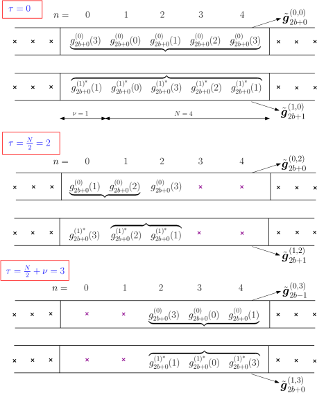
Illustrative examples for Proposition 1 are provided in Fig. 3 for the AL-OFDM signal with , , , , and . Note that the vector components are written based on (23)-(29), given in the appendix, and by taking into account the relationship between and . The uncorrelated and correlated samples are indicated by using ’’ and braces, respectively.
Based on results of Proposition 1, we define the following cross-correlation
| (4) |
where indicates the statistical expectation over the block, is an -length block with components , , the superscript denotes matrix transpose, and is the number of blocks.
By using Proposition 1, one can easily see that for , the cross-correlation for AL-OFDM and SM-OFDM signals is respectively given by
| (5) |
and
| (6) |
where is the variance of the modulated symbols222Note that based on the Parseval’s theorem, the variance of the modulated symbols is equal to the variance of the samples in the block at the output of the IFFT.. Note that the factor in (5) is due to the fact that correlation exists only between the -length blocks which belong to the same AL block. According to (5) and (6), provides a feature for the identification of the AL-OFDM and SM-OFDM signals.
Receive-side
Without loss of generality, we assume that the first intercepted sample corresponds to the start of an OFDM block; later in the paper, we will relax this assumption. Let us define the sequence , whose components are given by , , and further divide it into -length333We assume that the OFDM block length is known. Different algorithms in the literature, e.g., [33], can be combined with the proposed algorithm to blindly estimate the OFDM block length. blocks, i.e., , where , with
By using (2), the definition of the correlation in (4), (5), and (6), and taking into account the independence between the transmitted data symbols, noise, and channel coefficients, for it is straightforward to find that
| (7) |
and
| (8) |
where .
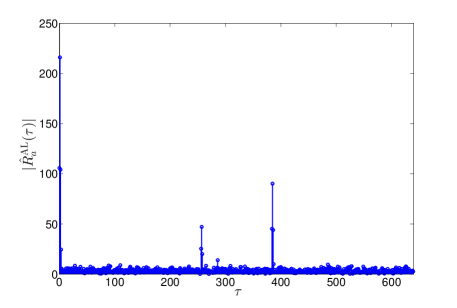
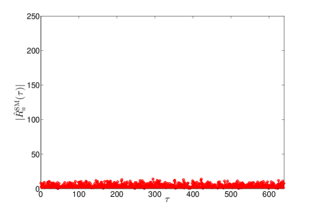
Fig. 4 shows the absolute value of the estimated cross-correlation, , , for both AL-OFDM and SM-OFDM signals with QPSK modulation, , , and over multipath Rayleigh fading channel with at SNR=10 dB. Note that the limited observation period results in non-zero, but statistically non-significant values for and at the null positions. The existence of the statistically significant peaks in will be used as a discriminating feature to identify AL-OFDM and SM-OFDM signals. It is worthy to mention that the first received sample does not have to correspond to the start of an OFDM block. In such a case, the peaks in Fig. 4 (a) will be cyclically shifted by the number of samples corresponding to the delay between the first received sample and the start of the first received OFDM block, which does not affect the discriminating feature.
III-B Discriminating feature and decision criterion ( case)
The identification of AL-OFDM and SM-OFDM signals relies on detecting whether statistically significant peaks are present or not in , . This can be formulated as a binary hypothesis testing problem, where under hypothesis (no peaks are detected) SM-OFDM is decided to be the received signal, whereas AL-OFDM signal is selected under hypothesis (peaks are detected). Here we propose a statistical test to detect the peak presence.
Without loss of generality, we assume that the number of observed samples, , corresponds to an integer number of OFDM blocks, 444If this not the case, zeros can be added after the observed samples to ensure this relation. Additionally, it is worth noting that the number of received blocks used for signal identification, , is finite.. In this case, can be estimated as
| (9) |
Following [34], can be represented as
| (10) |
where is a zero-mean random variable representing the estimation error, which vanishes asymptotically (). As shown in (7), under the assumption that the first received sample corresponds to the start of an OFDM block, exhibits peaks around , and . In general, if the first received sample corresponds to the th point in the OFDM block, the peaks in will be around , , and .
| (11) |
where is non-zero for , .
| (12) |
As such, if 555Henceforth, the superscript AL or SM is dropped in the cross-correlation, as this is not known at the receive-side. for at least one value of , the AL-OFDM signal is declared present ( is true); otherwise, the SM-OFDM signal is declared present ( is true). The proposed statistical test detects the presence of the non-zero value of as follows. For , we define as the value of that maximizes ,
| (13) |
Based on the results provided in (7), one can notice that for the AL-OFDM signal, will take values in the set . Depending on the value within this range, in order to eliminate all possible peak positions, we consider the set , with and . As such, for both AL-OFDM and SM-OFDM signals for the delay range . This result will be used in the definition of the test statistic to avoid the statistically significant peaks.
When the SM-OFDM signal is received (under hypothesis ), has an asymptotic complex Gaussian distribution with zero-mean and variance [34, 35]. Therefore, the normalized cross-correlation, , asymptotically follows a complex Gaussian distribution with zero-mean and variance equal to 2. Based on that, we define the function as
| (14) |
where is the cardinality of the set .666Note that in a practical implementation of the algorithm, knowledge of is not required; a reasonably large value is considered. However, this is significantly low when compared to and does not affect the algorithm performance. Note that the denominator in (14) is an estimate of the variance of under hypothesis , which converges to when goes to infinity. As such, has an asymptotic chi-square distribution with two degrees of freedom under hypothesis [36]. Accordingly, we define the test statistic as
| (15) |
Then we set a threshold, , to yield a desired probability of false alarm, , i.e., . Using the expression of the cumulative distribution function (CDF) of the chi-square distribution with two degrees of freedom [36], we can find that
| (16) |
Since , the threshold, , can be calculated for a given as
| (17) |
Finally, if , the AL-OFDM signal is decided to be received; otherwise, the SM-OFDM signal is selected. A summary of the proposed identification algorithm is given below.
III-C Discriminating feature and decision criterion ( case)
In the previous section we considered two receive antennas (); here, we generalize the proposed identification algorithm to . Basically, the cross-correlations between each pair of the receive antennas will be combined to improve the discriminating feature. Similar to (9), the cross-correlation between the th and th receive antennas, , can be estimated as
| (18) |
For each pair of receive antennas, the function , , is calculated as
| (19) |
and the functions for all pairs of receive antennas are combined as
| (20) |
Accordingly, the test statistic is defined as
| (21) |
As has an asymptotic chi-square distribution with two degrees of freedom under hypothesis , asymptotically follows the chi-square distribution with degrees of freedom, where is the number of the pairs of receive antennas. Hence, for a certain we set the threshold based on the CDF of this chi-square distribution, i.e.,
III-D Computational complexity
The computational complexity of the proposed algorithm is measured by the required number of floating point operations (flops) [39], which can be easily found to be equal to . For example, with , , , and , the proposed algorithm requires 61,505,280 flops. Practically speaking, a microprocessor with 79.992 Giga-flops777[online], available: http://download.intel.com/support/processors/corei7/sb/corei7-900d.pdf can perform the calculations needed for the proposed algorithm in approximately 769 sec.
IV Simulation results
IV-A Simulation setup
The identification performance of the proposed algorithm was evaluated using Monte Carlo simulations with 1000 trials for each signal type. The OFDM signals are generated based on the IEEE 802.11e standard, with a useful OFDM block duration of 91.4 sec and a subcarrier spacing of kHz. Unless otherwise mentioned, the modulation was QPSK, the number of OFDM subcarriers (2.5 MHz double-sided bandwidth), the cyclic prefix , the number of observed OFDM blocks , the number of receive antennas , and the probability of false alarm . Furthermore, the received signal was affected by a frequency selective Rayleigh fading channel888While a Rayleigh fading channel is considered here, it is worth noting that a similar performance is achieved under multipath Nakagami- fading conditions, as the distribution of the test statistic is similar under diverse channel conditions, as shown by simulations. consisting of statistically independent taps, with an exponential power delay profile [40], , where . A Butterworth filter was used at the receive-side to remove the out-of-band noise, and the SNR was considered at the output of this filter. The average probability of correct identification, , was employed as a performance measure, where is the estimated signal type.
IV-B Performance evaluation
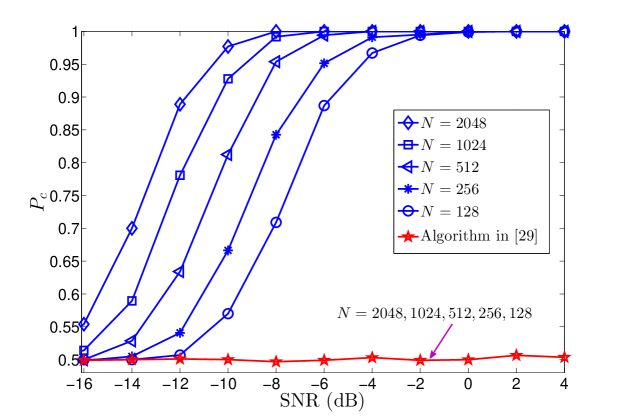
Fig. 5 shows the performance of the proposed algorithm in comparison with that in [29] for different numbers of OFDM subcarriers, . Apparently, the proposed algorithm outperforms the algorithm in [29], which basically fails; the reason is that the latter requires a large number of OFDM blocks to estimate the discriminating feature, e.g., simulation results show that is needed to reach at SNR = -4 dB.
In terms of computational complexity, the algorithm in [29] requires flops. If we compare the complexity of this algorithm and the proposed algorithm for given values of , , , and , the algorithm in [29] is less computationally demanding. For example, for , , , and , the former requires 257,280 flops, while the latter needs 61,505,280 flops. However, such a complexity comparison is not fair due to the difference in performance (as discussed above, based on results in Fig. 5). If we consider the values for which the algorithms reach at a given SNR, along with the fact that the time to make a decision consists of both observation and computing times, then it can be easily found that the algorithm in [29] requires a longer time for decision. For example, when a microprocessor with 79.992 Giga-flops is employed for computation, the algorithm in [29] needs 1.1428 sec to make a decision with at SNR= -4 dB (), whereas the proposed algorithm requires only 12.194 sec ().
Furthermore, it can be observed from Fig. 5 that the identification performance of the proposed algorithm significantly improves by increasing . This is because the peak values in are significantly enhanced, i.e., is proportional to as can be noticed from (7). This reflects on the discriminating feature and leads to identification performance improvement.
IV-C Effect of the number of OFDM blocks
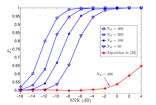
Fig. 6 shows the effect of the number of OFDM blocks, , on the average probability of correct identification, . A comparison with the algorithm in [29] for is also included. As expected, increasing enhances the performance of the proposed algorithm, as it leads to a better estimate of the cross-correlation, . Note that the proposed algorithm provides an excellent performance () at SNR = 0 dB and with a small number of blocks, , whereas the algorithm in [29] does not achieve a good performance even for .
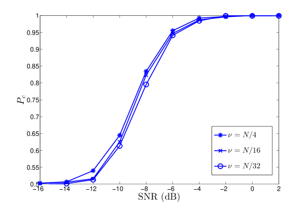
IV-D Effect of the cyclic prefix length
Fig. 7 shows the average probability of correct identification, , for , , and . One can notice that the performance slightly improves by increasing ; this is because under the hypothesis (the AL-OFDM signal), the peak values in slightly increase with . It is worth noting that the improvement obtained by increasing is more significant, as was seen in Fig. 5.
IV-E Effect of the number of receive antennas
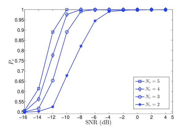
Fig. 8 illustrates the effect of the number of receive antennas, , on the average probability of correct identification, . It can be seen that the identification performance is improved by increasing . For example, with , an excellent performance is obtained at SNR dB, when compared with SNR dB for . However, the computational complexity increases by a factor of 10, according to results presented in Section III.D.
IV-F Effect of the modulation format
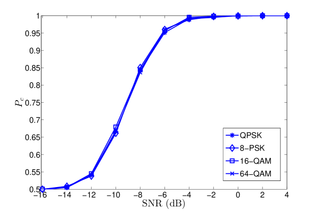
Fig. 9 presents the effect of the modulation format on the average probability of correct identification, . Clearly, it does not affect the performance of the proposed algorithm, as the peak values in do not depend on the modulation format, according to (7).
IV-G Effect of the timing offset
Perfect timing synchronization was assumed in the previous study. Here we evaluate the performance of the proposed algorithm in the presence of a timing offset. As mentioned in Section III, a timing offset equal to a multiple integer of the sampling period leads to a shift in the positions of the peaks by an amount corresponding to that offset; consequently, this does not affect the discriminating feature. On the other hand, when the timing offset is a fraction of the sampling period, its effect is modeled as a two path channel , where is the normalized timing offset [22]. Fig. 10 shows the average probability of correct identification, , for , and 0.5. The results indicate that while the performance slightly decreases at lower SNRs, it is not affected at higher SNRs. This can be explained, as the effect of can be considered as an additional noise component that affects the peaks in .
IV-H Effect of the frequency offset
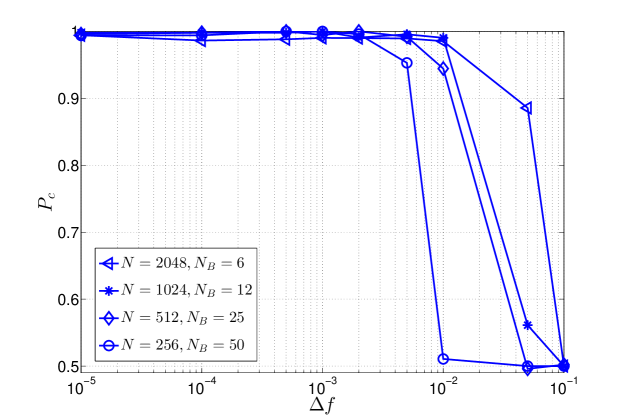
Fig. 11 presents the effect of the frequency offset normalized to the subcarrier spacing, , on the average probability of correct identification, , at SNR = 0 dB and for different values of and . Note that as the OFDM block duration is constant regardless of (see Section IV.A), the observation period increases with , which leads to an increased effect of the frequency offset on the performance. It is worth noting that a reduced number of OFDM blocks is required to achieve a good performance for a larger number of subcarriers, which results in a lower sensitivity to the frequency offset. Results in Fig. 11 show a good robustness for when and .
IV-I Effect of the Doppler frequency
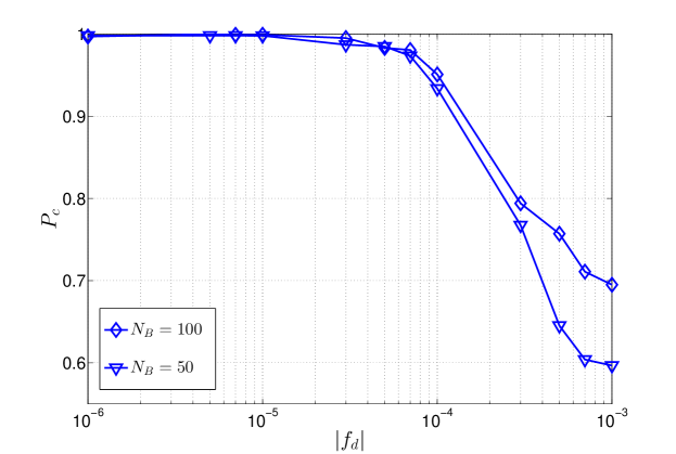
The previous analysis assumed constant channel coefficients over the observation period. Here, we consider the effect of the Doppler frequency on the performance of the proposed algorithm. Fig. 12 shows the average probability of correct identification, , versus the absolute value of the Doppler frequency normalized to the sampling rate, , at SNR dB and and 100. The results show a good robustness for .
IV-J Effect of the spatially correlated fading
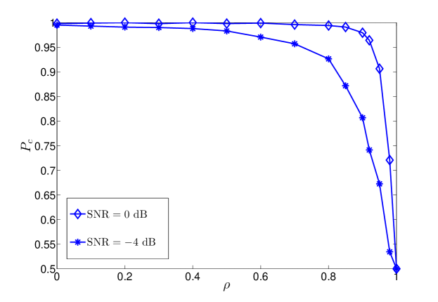
In the previous study, independent fading was considered. Here, we show the effect of the spatially correlated fading on the performance of the proposed algorithm. Fig. 13 shows the average probability of correct identification of the proposed algorithm, , versus the spatial correlation coefficient, , at SNR dB and 0 dB. As shown in (7), the channel coefficients affect the peak values in by the factor . At high values of , and , . As such, the discriminating peaks vanish and the identification performance degrades999It is worth noting that the same performance is obtained if the spatially correlated fading occurs at the transmit-side; in this case and , , at high values of the correlation coefficient.. As expected, the performance is more affected by spatially correlated fading at lower SNR.
V Conclusion
The identification of the AL-OFDM and SM-OFDM signals has been investigated in this paper. A new cross-correlation was developed, which provides an efficient feature for signal identification. Based on the statistical properties of the feature estimate, a novel criterion of decision was introduced. The proposed identification algorithm, which employs the aforementioned discriminating feature and decision criterion, provides an improved performance when compared with the previous work in the literature, at lower SNR and with reduced observation period. The algorithm has the advantages that it does not require channel and noise power estimation, modulation identification or timing synchronization. Furthermore, it exhibits a relatively low sensitivity to spatially correlated fading and frequency offset.
Appendix: Proof of Proposition 1
For the AL-OFDM signal, by using the definition of the ()-length blocks in the sequence (see Fig. 2 for the graphical illustration), one can easily express the samples of and respectively as
| (23) |
and
| (24) |
Based on (1), for the case of , it can be written that
| (25) |
and
| (26) |
By using that , , for AL-OFDM signal, and taking the complex conjugate of (26), it is straightforward that
| (27) |
It is easy to see that , only when . A few examples are given as follows: ; ; ; and . Hence, one can notice that for , and for . This leads to the result shown in (3a).
For , it is straightforward that and belong to the (same) th AL block for . Moreover, based on the aforementioned results regarding and , one can see that if and satisfy and . If and , then , . This directly leads to the result in (3b). On the other hand, if (either equal to or ), then , ; this leads to the case of discussed above. Furthermore, if and , then , which is out of range ().
Moreover, also for the AL-OFDM signal, one can similarly express the samples of and respectively as
| (28) |
and
| (29) |
Accordingly, and belong to the (same) th AL block for . By using the same analysis as above, one can prove results in (3c).
References
- [1] O. A. Dobre, A. Abdi, Y. Bar-Ness, and W. Su, “Survey of automatic modulation classification techniques: Classical approaches and new trends,” IET Commun., vol. 1, pp. 137–156, Apr. 2007.
- [2] D. Cabric, “Addressing feasibility of cognitive radios,” IEEE Signal Process. Mag., vol. 25, pp. 85–93, Nov. 2008.
- [3] J. L. Xu, W. Su, and M. Zhou, “Software-defined radio equipped with rapid modulation recognition,” IEEE Trans. Veh. Technol., vol. 59, pp. 1659–1667, May 2010.
- [4] H.-C. Wu, M. Saquib, and Z. Yun, “Novel automatic modulation classification using cumulant features for communications via multipath channels,” IEEE Trans. Wireless Commun., vol. 7, pp. 3098–3105, Aug. 2008.
- [5] W. Su, “Feature space analysis of modulation classification using very high-order statistics,” IEEE Commun. Lett., vol. 17, pp. 1688–1691, Sep. 2013.
- [6] W. Su, J. L. Xu, and M. Zhou, “Real-time modulation classification based on maximum likelihood,” IEEE Commun. Lett., vol. 12, pp. 801–803, Nov. 2008.
- [7] O. A. Dobre, M. Oner, S. Rajan, and R. Inkol, “Cyclostationarity-based robust algorithms for QAM signal identification,” IEEE Commun. Lett., vol. 16, pp. 12–15, Jan. 2012.
- [8] D. Grimaldi, S. Rapuano, and L. De Vito, “An automatic digital modulation classifier for measurement on telecommunication networks,” IEEE Trans. Instrum. Meas., vol. 56, pp. 1711–1720, Oct. 2007.
- [9] Q. Zhang, O. A. Dobre, Y. Eldemerdash, S. Rajan, and R. Inkol, “Second-order cyclostationarity of BT-SCLD signals: Theoretical developments and applications to signal classification and blind parameter estimation,” IEEE Trans. Wireless Commun., vol. 12, pp. 1501–1511, Apr. 2013.
- [10] A. Bouzegzi, P. Ciblat, and P. Jallon, “New algorithms for blind recognition of OFDM based systems,” Elsevier Signal Processing, vol. 90, pp. 900–913, Mar. 2010.
- [11] A. Al-Habashna, O. A. Dobre, R. Venkatesan, and D. C. Popescu, “Second-order cyclostationarity of mobile WiMAX and LTE OFDM signals and application to spectrum awareness in cognitive radio systems,” IEEE J. Sel. Topics Signal Process., vol. 6, pp. 26–42, Feb. 2012.
- [12] T. Xia and H.-C. Wu , “Blind identification of nonbinary LDPC codes using average LLR of syndrome a posteriori probability,” IEEE Commun. Lett., vol. 17, pp. 1301–1304, Jul. 2013.
- [13] ——, “Novel blind identification of LDPC codes using average LLR of syndrome a posteriori probability,” IEEE Trans. Signal Process., vol. 62, pp. 632–640, Feb. 2014.
- [14] ——, “Joint blind frame synchronization and encoder identification for low-density parity-check codes,” IEEE Commun. Lett., vol. 18, pp. 352–355, Feb. 2014.
- [15] H.-C. Wu, X. Huang, and D. Xu, “Pilot-free dynamic phase and amplitude estimations for wireless ICI self-cancellation coded OFDM systems,” IEEE Trans. Broadcast., vol. 51, pp. 94–105, Mar. 2005.
- [16] L. Korowajczuk, LTE, WiMAX and WLAN Network Design, Optimization and Performance Analysis. Wiley, 2011.
- [17] M. Shi, Y. Bar-Ness, and W. Su, “Adaptive estimation of the number of transmit antennas,” in Proc. IEEE MILCOM, 2007, pp. 1–5.
- [18] O. Somekh, O. Simeone, Y. Bar-Ness, and W. Su, “Detecting the number of transmit antennas with unauthorized or cognitive receivers in MIMO systems,” in Proc. IEEE MILCOM, 2007, pp. 1–5.
- [19] K. Hassan, I. Dayoub, W. Hamouda, C. N. Nzeza, and M. Berbineau, “Blind digital modulation identification for spatially-correlated MIMO systems,” IEEE Trans. Wireless Commun., vol. 11, pp. 683–693, Feb. 2012.
- [20] V. Choqueuse, S. Azou, K. Yao, and G. Burel, “ Blind modulation recognition for MIMO systems,” J. Military Technical Academy Review, vol. XIX, pp. 183–196, Jun. 2009.
- [21] M. S. Mühlhaus, M. Öner, O. A. Dobre, and F. K. Jondral, “A low complexity modulation classification algorithm for MIMO systems,” IEEE Commun. Lett., vol. 17, pp. 1881–1884, Oct. 2013.
- [22] V. Choqueuse, K. Yao, L. Collin, and G. Burel, “Hierarchical space-time block code recognition using correlation matrices,” IEEE Trans. Wireless Commun., vol. 7, pp. 3526–3534, Sep. 2008.
- [23] V. Choqueuse, M. Marazin, L. Collin, K. C. Yao, and G. Burel, “Blind recognition of linear space–time block codes: A likelihood-based approach,” IEEE Trans. Signal Process., vol. 58, pp. 1290–1299, Mar. 2010.
- [24] M. Marey, O. A. Dobre, and R. Inkol, “Classification of space-time block codes based on second-order cyclostationarity with transmission impairments,” IEEE Trans. Wireless Commun., vol. 11, pp. 2574–2584, Jul. 2012.
- [25] M. Luo, L. Gan, and L. Li, “Blind recognition of space-time block code using correlation matrices in a high dimensional feature space,” J. Inf. Comput. Sci, vol. 9, pp. 1469–1476, Jun. 2012.
- [26] G. Qian, L. Li, M. Luo, H. Liao, and H. Zhang, “Blind recognition of space-time block code in MISO system,” EURASIP JWCN, vol. 1, pp. 164–176, Jun. 2013.
- [27] Y. A. Eldemerdash, M. Marey, O. A. Dobre, G. Karagiannidis, and R. Inkol, “Fourth-order statistics for blind classification of spatial multiplexing and Alamouti space-time block code signals,” IEEE Trans. Commun., vol. 61, pp. 2420–2431, Jun. 2013.
- [28] H. Agirman-Tosun, Y. Liu, A. Haimovich, O. Simeone, W. Su, J. Dabin, and E. Kanterakis, “Modulation classification of MIMO-OFDM signals by independent component analysis and support vector machines,” in Proc. IEEE ASILOMAR, 2011, pp. 1903–1907.
- [29] M. Marey, O. A. Dobre, and R. Inkol, “Novel algorithm for STBC-OFDM identification in cognitive radios,” in Proc. IEEE ICC, 2013, pp. 2770–2774.
- [30] M. Marey, O. Dobre, and R. Inkol, “Blind STBC identification for multiple-antenna OFDM systems,” IEEE Trans. Commun., vol. 62, pp. 1554–1567, May 2014.
- [31] E. Karami and O. A. Dobre, “Identification of SM-OFDM and AL-OFDM signals based on their second-order cyclostationarity,” IEEE Trans. Veh. Technol., DOI: 10.1109/TVT.2014.2326107, 2014.
- [32] Y. G. Li, J. H. Winters, and N. R. Sollenberger, “MIMO-OFDM for wireless communications: signal detection with enhanced channel estimation,” IEEE Trans. Commun., vol. 50, pp. 1471–1477, Sep. 2002.
- [33] A. Punchihewa, V. K. Bhargava, and C. Despins, “Blind estimation of OFDM parameters in cognitive radio networks,” IEEE Trans. Wireless Commun., vol. 10, pp. 733–738, Mar. 2011.
- [34] S. M. Kay, Fundamentals of Statistical Signal Processing: Estimation Theory . Prentice Hall, 1993.
- [35] D. R. Brillinger, Time Series: Data Analysis and Theory. McGraw-Hills, 1981.
- [36] A. Papoulis and S. Pillai, Probability, Random Variables and Stochastic Processes. McGraw-Hill, 2001.
- [37] M. K. Simon, Probability Distributions Involving Gaussian Random Variables: A Handbook for Engineers and Scientists. Springer, 2007.
- [38] J. Stoer and R. Bulirsch, Introduction to Numerical Analysis. Springer, 2002.
- [39] D. Watkins, Fundamentals of Matrix Computations. Wiley, 2002.
- [40] M. Patzold, A. Szczepanski, and N. Youssef, “Methods for modeling of specified and measured multipath power-delay profiles,” IEEE Trans. Veh. Technol., vol. 51, pp. 978–988, Sep. 2002.