FIMP and Muon ($g-2$) in a U$(1)_{L_{\mu}-L_{\tau}}$ Model

Abstract

The tightening of the constraints on the standard thermal WIMP scenario has forced physicists to propose alternative dark matter (DM) models. One of the most popular alternate explanations of the origin of DM is the non-thermal production of DM via freeze-in. In this scenario the DM never attains thermal equilibrium with the thermal soup because of its feeble coupling strength ($\sim 10^{-12}$) with the other particles in the thermal bath and is generally called the Feebly Interacting Massive Particle (FIMP). In this work, we present a gauged U(1)${}_{L_{\mu}-L_{\tau}}$ extension of the Standard Model (SM) which has a scalar FIMP DM candidate and can consistently explain the DM relic density bound. In addition, the spontaneous breaking of the U(1)${}_{L_{\mu}-L_{\tau}}$ gauge symmetry gives an extra massive neutral gauge boson $Z_{\mu\tau}$ which can explain the muon ($g-2$) data through its additional one-loop contribution to the process. Lastly, presence of three right-handed neutrinos enable the model to successfully explain the small neutrino masses via the Type-I seesaw mechanism. The presence of the spontaneously broken U(1)${}_{L_{\mu}-L_{\tau}}$ gives a particular structure to the light neutrino mass matrix which can explain the peculiar mixing pattern of the light neutrinos.

I Introduction

The presence of Dark Matter (DM) is a well established truth and demands the extension of the Standard Model (SM). Starting from the time of Zwicky (who examined the coma-cluster in 1933 and gave the prediction of excess matter) till now, many collaborations have reported the existence of DM. The most prominent examples are, flatness of galaxy rotation curve Sofue:2000jx , gravitational lensing Bartelmann:1999yn and the Bullet cluster observed by NASA’s Chandra satellite Clowe:2003tk . In the last one decade, satellite borne experiments like WMAP (Wilkinson Massive Anisotropy Probe) Hinshaw:2012aka and Planck Ade:2015xua not only confirmed the existence of DM but also measured the amount of DM present in the Universe with an unprecedented accuracy. However, the particle content of dark matter as well as its interaction strength with the visible world are two questions which remain unresolved. Depending on their production mechanism in the early Universe, the dark matter particles can be classified into two groups. The first group is the thermal dark matter. These class of particles were produced thermally and maintained their thermal as well as chemical equilibrium with the thermal bath. They eventually decoupled from the plasma when their interaction rates became less than the expansion rate of the Universe. Being relic particles, their comoving number density froze to a particular value. This is known as the usual freeze-out mechanism Gondolo:1990dk ; Srednicki:1988ce . The dark matter candidates which were produced through the freeze-out scenario are usually called the Weakly Interacting Massive Particle or WIMP Gondolo:1990dk ; Srednicki:1988ce . These types of particles have weak scale interaction cross section and their signatures are expected to be seen at various ongoing direct detection experiments like LUX Akerib:2016vxi ; Akerib:2015rjg and XENON-1T Aprile:2015uzo . However, the direct detection experiments are yet to find any real signal of dark matter particles. This forces us to look for other types of dark matter particles which can be an alternative to the WIMP scenario. One such class of dark matter candidates is the Feebly Interacting Massive Particle or FIMP Hall:2009bx ; Yaguna:2011qn ; Molinaro:2014lfa ; Biswas:2015sva ; Merle:2015oja ; Shakya:2015xnx ; Biswas:2016bfo ; Konig:2016dzg . The interaction rates of these particles are so feeble that they never attained thermal equilibrium with the thermal bath. As a result, their initial number densities were negligible compared to others which were in thermal equilibrium. As the Universe cooled down, they were produced predominantly from the decays of heavy particles. If the decaying mother particles are in thermal equilibrium at the early stage of the Universe, the production of dark matter particles from a particular decay mode is expected to be maximum around a temperature equal to the mass of the corresponding decaying particle. In principle, FIMP can also be produced from the annihilation of SM particles and other heavy particles (beyond SM) as well. The production mechanism of FIMP is known as freeze-in Hall:2009bx which is opposite to the freeze-out scenario. Unlike the freeze-out mechanism, in case of freeze-in the comoving number density and hence the relic density of a FIMP is directly proportional to its couplings with other particles. Since the interaction strength of a FIMP is extremely weak, thus one can evade all the constraints arising from the direct detection experiments.

Besides the dark sector, the other puzzles which require the extension of the SM are the observation of neutrino mass Ahmad:2002jz , discrepancy in the anomalous magnetic moment of muon ($g-2$) Bennett:2006fi from its SM prediction and also the baryon asymmetry of the Universe Fukugita:1986hr . The existence of extremely small neutrino masses were first confirmed by the Super-Kamiokande collaboration Fukuda:1998mi from the observation of neutrino flavor oscillations in atmospheric neutrino data. Thereafter, many outstanding neutrino experiments like SNO Ahmad:2002jz , KamLand Eguchi:2002dm , Daya Bay An:2015nua , RENO RENO:2015ksa , Double Chooz Abe:2014bwa , T2K Abe:2015awa ; Salzgeber:2015gua and NO$\nu$A Adamson:2016tbq ; Adamson:2016xxw have precisely measured the two mass squared differences and three mixing angles between different neutrino flavours.

In the present work, we try to explain the existence of dark matter, tiny nature of neutrino masses, their intergenerational mixing angles and muon ($g-2$) anomaly simultaneously within the framework of our proposed model. Since we already know that the SM is unable to address these issues, we have to think of a beyond Standard Model (BSM) scenario. There are many well motivated extensions of the SM like SUSY, two Higgs doublet model, extension of the SM gauge group by extra U(1) and many more. In this work we have extended the SM gauge group by a local ${\rm U(1)}_{L_{\mu}-L_{\tau}}$ symmetry Choubey:2004hn ; Biswas:2016yan ; Altmannshofer:2016jzy . Therefore, the complete gauge group in this model is ${\rm SU}(2)_{\rm L}\times{\rm U}(1)_{\rm Y}\times{\rm U(1)}_{L_{\mu}-L_{\tau}}$. Since we are increasing the SM gauge group by a local ${\rm U(1)}_{L_{\mu}-L_{\tau}}$ symmetry, we must check the cancellation of axial vector anomaly Adler:1969gk ; Bardeen:1969md and mixed gravitational-gauge anomaly Delbourgo:1972xb ; Eguchi:1976db . The advantage of the ${\rm U(1)}_{L_{\mu}-L_{\tau}}$ extension is that these anomalies cancel automatically between the second and third generations He:1990pn ; He:1991qd ; Ma:2001md of SM fermions.

We also extend the particle content of the SM and include three right-handed neutrinos and two SM gauge singlet scalars. The new particles are given appropriate ${\rm U(1)}_{L_{\mu}-L_{\tau}}$ charge. One of the scalars picks up a Vacuum Expectation Value (VEV) breaking ${\rm U(1)}_{L_{\mu}-L_{\tau}}$ symmetry spontaneously, while the other does not take any VEV. The ${\rm U(1)}_{L_{\mu}-L_{\tau}}$ charge $n_{\mu\tau}$ of the other scalar $\phi_{DM}$ is chosen in such a way that it remains stable even after ${\rm U(1)}_{L_{\mu}-L_{\tau}}$ breaking and becomes a dark matter candidate. The new gauge boson $Z_{\mu\tau}$ after spontaneous breaking of ${\rm U(1)}_{L_{\mu}-L_{\tau}}$ becomes massive and gives additional contribution to the muon $(g-2)$, helping reconcile the observed data with the theoretical prediction in this model. The three right-handed neutrinos carry Majorana masses and give rise to light neutrino mass matrix via the Type-I seesaw mechanism. In our earlier work in Ref. Biswas:2016yan , we showed that our model can explain the nonzero neutrino masses and their intergenerational mixing angles. Also in that work, we considered the scalar field $\phi_{DM}$ as a WIMP type dark matter candidate and checked its viability in various direct detection experiments. We found that all the existing constraints are satisfied around the resonance regions, where the mediator mass is nearly equal to twice of dark matter mass.

In this work, we show that $\phi_{DM}$ could serve as a FIMP type dark matter candidate in this ${\rm U(1)}_{L_{\mu}-L_{\tau}}$ extension of the SM. All particles of our model including the additional scalar $h_{2}$, $Z_{\mu\tau}$ and the three right-handed neutrinos are in thermal equilibrium in the early Universe except $\phi_{DM}$. In order to make this possible, $\phi_{DM}$ must be feebly interacting with other particles. We choose its couplings with the visible sector to be extremely small (see Section II and IV for detailed discussions) such that it remains out of equilibrium throughout its evolution in the early Universe . We compute the relic density of $\phi_{DM}$ by solving the Boltzmann equation where we consider all the possible production modes of $\phi_{DM}$ from the decays as well as the annihilations of SM and BSM particles. We find that in our model, $\phi_{DM}$ is produced not only from the decays of $h_{1}$ and $h_{2}$, but also from the pair annihilation of $N_{i}$ ($i=2$, 3) mediated by the extra neutral gauge boson $Z_{\mu\tau}$. Therefore, the dark matter phenomenology is intricately intertwined with the phenomenology of neutrino masses and muon $(g-2)$.

Rest of the paper is organised in the following way. In Section II we describe the model in detail. In Section III we discuss muon ($g-2$) and neutrino masses and mixings. The Boltzmann equation for FIMP considering all possible production channels is given in Section IV. Our main results are presented in Section V. Finally, we summarise the present work in Section VI. All the relevant decay widths and annihilation cross sections are given in Appendices A and B.

II Model

We have considered the ${\rm U(1)}_{L_{\mu}-L_{\tau}}$ extension of the SM, where $L_{\mu}$ and $L_{\tau}$ are the muon and tau lepton numbers, respectively. Hence, the complete gauge group of the minimally extended SM is ${\rm SU}(2)_{\rm L}\times{\rm U}(1)_{\rm Y}\times{\rm U(1)}_{L_{\mu}-L_{\tau}}$. The particle content of our model is given in Tables 1 and 2.

Gauge Group ${\rm SU(2)}_{\rm L}$ ${\rm U(1)}_{\rm Y}$

Baryon Fields $Q_{L}^{i}=(u_{L}^{i},d_{L}^{i})^{T}$ $u_{R}^{i}$ $d_{R}^{i}$ $2$ $1$ $1$ $1/6$ $2/3$ $-1/3$

Lepton Fields $L_{L}^{i}=(\nu_{L}^{i},e_{L}^{i})^{T}$ $e_{R}^{i}$ $N_{R}^{i}$ $2$ $1$ $1$ $-1/2$ $-1$ $0$

Scalar Fields $\phi_{h}$ $\phi_{H}$ $\phi_{DM}$ $2$ $1$ $1$ $1/2$ $0$ $0$

Table 1: Charges of all particles under SM gauge group.

Gauge Group ${\rm U(1)}_{L_{\mu}-L_{\tau}}$

Baryonic Fields $(Q^{i}_{L},u^{i}_{R},d^{i}_{R})$ $0$

Lepton Fields $(L_{L}^{e},e_{R},N_{R}^{e})$ $(L_{L}^{\mu},\mu_{R},N_{R}^{\mu})$ $(L_{L}^{\tau},\tau_{R},N_{R}^{\tau})$ $0$ $1$ $-1$

Scalar Fields $\phi_{h}$ $\phi_{H}$ $\phi_{DM}$ $0$ $1$ $n_{\mu\tau}$

Table 2: Charges of all particles under ${\rm U(1)}_{L_{\mu}-L_{\tau}}$ gauge group.

The Lagrangian for this model is as follows,

$$\mathcal{L} = \mathcal{L}_{SM}+\mathcal{L}_{N}+\mathcal{L}_{DM}+(D_{\mu}\phi_{H})^{\dagger}(D^{\mu}\phi_{H})-V(\phi_{h},\phi_{H})-\frac{1}{4}F_{\mu\tau}^{\alpha\beta}{F_{\mu\tau}}_{\alpha\beta}\,,$$ (1)

where $\mathcal{L}_{SM}$ represents the Lagrangian of SM and $\mathcal{L}_{N}$ is the Lagrangian for the RH neutrinos which contains its kinetic energy terms, mass terms and Yukawa terms with the SM leptons doublets. The expression of $\mathcal{L}_{N}$ is,

$$\mathcal{L}_{N} = \sum_{\alpha=e,\,\mu,\,\tau}\frac{i}{2}\bar{N_{\alpha}}\gamma^{\mu}D_{\mu}N_{\alpha}-\dfrac{1}{2}\,M_{ee}\,\bar{N_{e}^{c}}N_{e}-\dfrac{1}{2}\,M_{\mu\tau}\,(\bar{N_{\mu}^{c}}N_{\tau}+\bar{N_{\tau}^{c}}N_{\mu})$$ (2)

$$-\dfrac{1}{2}\,h_{e\mu}(\bar{N_{e}^{c}}N_{\mu}+\bar{N_{\mu}^{c}}N_{e})\phi_{H}^{\dagger}-\dfrac{1}{2}\,h_{e\tau}(\bar{N_{e}^{c}}N_{\tau}+\bar{N_{\tau}^{c}}N_{e})\phi_{H}$$

$$-\sum_{\alpha=e,\,\mu,\,\tau}y_{\alpha}\bar{L_{\alpha}}\tilde{\phi_{h}}N_{\alpha}+h.c.\,$$

where $\tilde{\phi_{h}}=i\,\sigma_{2}\phi^{*}_{h}$ and the quantities $M_{\mu\tau}$, $M_{ee}$ have dimension of mass while the Yukawa couplings $h_{e\mu}$, $h_{e\tau}$ and $y_{\alpha}$s are dimensionless constants. In Eq. (1), $\mathcal{L}_{DM}$ part is the dark matter Lagrangian which contains the kinetic term of the dark matter candidate $\phi_{DM}$ and the interaction terms of $\phi_{DM}$ with the SM-like Higgs ($\phi_{h}$) and the extra Higgs ($\phi_{H}$). The expression of the $\mathcal{L}_{DM}$ is as follows,

$$\mathcal{L}_{DM} = (D^{\mu}\phi_{DM})^{\dagger}(D_{\mu}\phi_{DM})-\mu_{DM}^{2}\phi_{DM}^{\dagger}\phi_{DM}-\lambda_{DM}(\phi_{DM}^{\dagger}\phi_{DM})^{2}$$ (3)

$$-\lambda_{Dh}(\phi_{DM}^{\dagger}\phi_{DM})(\phi_{h}^{\dagger}\phi_{h})-\lambda_{DH}(\phi_{DM}^{\dagger}\phi_{DM})(\phi_{H}^{\dagger}\phi_{H})\,.$$

The fourth term in Eq. (1) represents the kinetic term of the extra Higgs singlet $\phi_{H}$. The potential $V(\phi_{h},\phi_{H})$ contains the quadratic and quartic interactions of $\phi_{H}$ and the interaction term between $\phi_{h}$ and $\phi_{H}$. The potential $V(\phi_{h},\phi_{H})$ has the following form,

$$V(\phi_{h},\phi_{H})=\mu_{H}^{2}\phi_{H}^{\dagger}\phi_{H}+\lambda_{H}(\phi_{H}^{\dagger}\phi_{H})^{2}+\lambda_{hH}(\phi_{h}^{\dagger}\phi_{h})(\phi_{H}^{\dagger}\phi_{H})\,.$$ (4)

The last term in the Eq. (1) is the kinetic energy term of the extra gauge boson Z_μτ in terms of the field strength tensor $F^{\alpha\beta}_{\mu\tau}$ which has the following form, $F_{\mu\tau}^{\alpha\beta}=\partial^{\alpha}Z_{\mu\tau}^{\beta}-\partial^{\beta}Z_{\mu\tau}^{\alpha}.$ We can write down the generic form of the covariant derivative which are appearing in the Eqs. (1)-(3) is,

$$D_{\nu}X=(\partial_{\nu}+i\,g_{\mu\tau}\,Q_{\mu\tau}(X)\,{Z_{\mu\tau}}_{\nu})\,X\,,$$ (5)

where $X$ is any SM singlet field which has ${\rm U(1)}_{L_{\mu}-L_{\tau}}$ charge $Q_{\mu\tau}(X)$ (see Table 2) and $g_{\mu\tau}$ is the gauge coupling of the ${\rm U(1)}_{L_{\mu}-L_{\tau}}$ gauge group. The ${\rm U(1)}_{L_{\mu}-L_{\tau}}$ symmetry breaks spontaneously once $\phi_{H}$ picks up a VEV and consequently the extra gauge field becomes massive with mass term $M_{Z_{\mu\tau}}=g_{\mu\tau}\,v_{\mu\tau}$. In the unitary gauge, $\phi_{h}$ and $\phi_{H}$ take the following form after spontaneous breaking of the ${\rm SU}(2)_{\rm L}\times{\rm U}(1)_{\rm Y}\times{\rm U(1)}_{L_{\mu}-L_{\tau}}$ gauge symmetry,

$$\phi_{h}=\begin{pmatrix}0\\ \dfrac{v+H}{\sqrt{2}}\end{pmatrix}\,,\,\,\,\,\,\,\,\,\,\phi_{H}=\begin{pmatrix}\dfrac{v_{\mu\tau}+H_{\mu\tau}}{\sqrt{2}}\end{pmatrix}\,,$$ (6)

where $v$ and $v_{\mu\tau}$ are the VEVs of $\phi_{h}$ and $\phi_{H}$ respectively. The presence of the mutual interaction between $\phi_{h}$ and $\phi_{H}$ in Eq. (4) induces the mixing between $H$ and $H_{\mu\tau}$. Hence, the scalar mixing matrix has the following form,

$$\mathcal{M}^{2}_{scalar}=\left(\begin{array}[]{cc}2\lambda_{h}\,v^{2}\nobreak\leavevmode\nobreak\leavevmode&\leavevmode\nobreak\ \leavevmode\nobreak\ \lambda_{hH}\,v_{\mu\tau}\,v\\ \nobreak\leavevmode\nobreak\leavevmode\hfil&\nobreak\leavevmode\nobreak\leavevmode\hfil\\ \lambda_{hH}\,v_{\mu\tau}\,v\nobreak\leavevmode\nobreak\leavevmode&\leavevmode\nobreak\ \leavevmode\nobreak\ 2\lambda_{H}\,v_{\mu\tau}^{2}\end{array}\right)\,\,.$$ (10)

We see from the expression of $\mathcal{M}^{2}_{scalar}$ that if we take $\lambda_{hH}=0$, then $H$ and $H_{\mu\tau}$ can represent the physical states (zero mixing between $H$ and $H_{\mu\tau}$). But in our case, $\lambda_{hH}\neq 0$ and therefore, we need to introduce two physical states in the following way,

$$h_{1} = H\cos\alpha+H_{\mu\tau}\sin\alpha\,,$$

$$h_{2} = -H\sin\alpha+H_{\mu\tau}\cos\alpha\,,$$ (11)

where $\alpha$ is the mixing angle. The above mixing matrix becomes diagonal with respect to the physical states $h_{1}$, $h_{2}$ and the eigenvalues of $\mathcal{M}^{2}_{scalar}$ represent the mass terms $M_{h_{1}}$ and $M_{h_{2}}$ of the scalar fields $h_{1}$ and $h_{2}$ respectively. In this work, we choose $h_{1}$ as the SM-like Higgs boson. The quartic couplings $\lambda_{h}$, $\lambda_{H}$ and $\lambda_{hH}$ can be expressed in terms of $M_{h_{1}}$, $M_{h_{2}}$, VEVs ($v$, $v_{\mu\tau}$) and mixing angle ($\alpha$) in the following way,

$$\lambda_{H} = \dfrac{M_{h_{2}}^{2}+M_{h_{1}}^{2}-(M_{h_{1}}^{2}-M_{h_{2}}^{2})\cos 2\alpha}{4\,v_{\mu\tau}^{2}}\,,$$

$$\lambda_{h} = \dfrac{M_{h_{2}}^{2}+M_{h_{1}}^{2}-(M_{h_{2}}^{2}-M_{h_{1}}^{2})\cos 2\alpha}{4\,v^{2}}\,,$$

$$\lambda_{hH} = -\dfrac{(M_{h_{2}}^{2}-M_{h_{1}}^{2})\cos\alpha\sin\alpha}{v\,v_{\mu\tau}}\,.$$ (12)

After symmetry breaking, mass of the dark matter is,

$$M_{DM}^{2}=\mu^{2}_{DM}+\dfrac{\lambda_{Dh}\,v^{2}}{2}+\dfrac{\lambda_{DH}\,v_{\mu\tau}^{2}}{2}\,.$$ (13)

In the present scenario, two of the three scalars take VEVs while the third one does not, i.e., $\langle\phi_{h}\rangle=\dfrac{v}{\sqrt{2}}$, $\langle\phi_{H}\rangle=\dfrac{v_{\mu\tau}}{\sqrt{2}}$ and $\langle\phi_{DM}\rangle=0$. This requires

$$\mu^{2}_{h}<0,\,\,\,\mu^{2}_{H}<0\,\,\text{and}\,\,\,\mu^{2}_{DM}>0.$$ (14)

In addition, the stability of the vacuum requires Biswas:2016ewm the following constraints on the quartic couplings of the scalar fields,

$$\lambda_{h}\geq 0,\lambda_{H}\geq 0,\lambda_{DM}\geq 0,$$

$$\lambda_{hH}\geq-2\sqrt{\lambda_{h}\,\lambda_{H}},$$

$$\lambda_{Dh}\geq-2\sqrt{\lambda_{h}\,\lambda_{DM}},$$

$$\lambda_{DH}\geq-2\sqrt{\lambda_{H}\,\lambda_{DM}},$$

$$\sqrt{\lambda_{hH}+2\sqrt{\lambda_{h}\,\lambda_{H}}}\sqrt{\lambda_{Dh}+2\sqrt{\lambda_{h}\,\lambda_{DM}}}\sqrt{\lambda_{DH}+2\sqrt{\lambda_{H}\,\lambda_{DM}}}$$

$$+2\,\sqrt{\lambda_{h}\lambda_{H}\lambda_{DM}}+\lambda_{hH}\sqrt{\lambda_{DM}}+\lambda_{Dh}\sqrt{\lambda_{H}}+\lambda_{DH}\sqrt{\lambda_{h}}\geq 0\,\,\,\,.$$ (15)

Besides the lower limit, there is an upper limit on the quartic couplings and the Yukawa couplings due to the perturbative regime, constraining them to be less than $4\pi$ and $\sqrt{4\pi}$, respectively.

III Muon $(g-2)$ and neutrino mass

In our previous work Biswas:2016yan we studied in detail the muon ($g-2$) and neutrino mass phenomenology in the framework of present model. The difference here with the previous work is that here we wish to produced the dark matter via the freeze-in mechanism instead of freeze-out, as in Biswas:2016yan . Our aim is to simultaneously explain the dark matter relic abundance as well as the muon ($g-2$). The region of the $g_{\mu\tau}$ - $M_{Z_{\mu\tau}}$ parameter space that can explain the muon ($g-2$) has been shown in Altmannshofer:2014pba . This allowed region is seen to be very small and mostly constrained by the neutrino trident process experiments such as CHARM-II, CCFR Geiregat:1990gz ; Mishra:1991bv and 4-leptons decay Altmannshofer:2014pba .

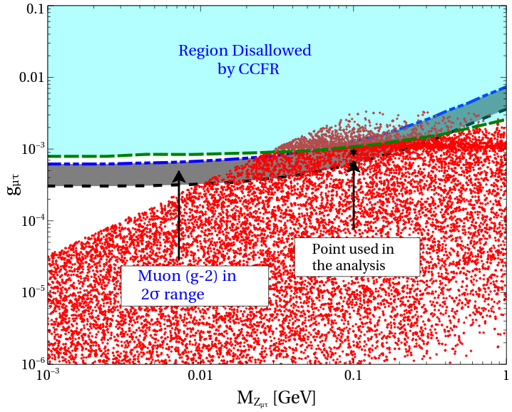
Figure 1: Bounds in the $g_{\mu\tau}$ - $M_{Z_{\mu\tau}}$ plane from different experiments and allowed region to satisfy relic density (red dots) and muon ($g-2$) excess in 2 $\sigma$ range (grey shaded region).

In determining the allowed parameter space for the present model, we have considered the relic density constraint Ade:2015xua and also the bound on invisible decay width of SM-like Higgs Khachatryan:2016vau . The one loop contribution Gninenko:2001hx ; Baek:2001kca to muon ($g-2$) for the ${\rm U(1)}_{L_{\mu}-L_{\tau}}$ gauge boson Z_μτ mediated diagram is given by,

$$\Delta a_{\mu}(Z_{\mu\tau})=\dfrac{g_{\mu\tau}^{2}}{8\pi^{2}}\int_{0}^{1}dx\dfrac{2x(1-x)^{2}}{(1-x)^{2}+rx}\,,$$ (16)

where, $r=(M_{Z_{\mu\tau}}/m_{\mu})^{2}$, $m_{\mu}$ being the muon mass. The discrepancy between the observed and SM predicted value Jegerlehner:2009ry of muon ($g-2$) is,

$$\Delta a_{\mu}=a_{\mu}^{\rm exp}-a_{\mu}^{\rm th}=(29.0\pm 9.0)\times 10^{-10}\,.$$ (17)

In Fig. 1 we show the allowed and disfavoured regions in the $g_{\mu\tau}$-$M_{Z_{\mu\tau}}$ plane. The region above the green dashed line is ruled out by the neutrino trident experiment CCFR Altmannshofer:2014pba . The grey region inside the blue dashed-dotted line and black dashed line can explain the ($g-2$) anomaly in $\pm$2$\sigma$ range Altmannshofer:2014pba . As will be discussed in much detail later, the red dots in this figure span the parameter region which can satisfy the dark matter relic abundance (cf. Eq. (35)). We see that for $g_{\mu\tau}\geq 3\times 10^{-3}$ no red points exist because the contribution from the $Z_{\mu\tau}$ mediated diagram to the relic abundance becomes too large. See Appendix A, for the expression of cross section of $\bar{N_{i}}\,N_{i}\rightarrow\phi_{DM}^{\dagger}\phi_{DM}$, $i=2,3$. The region of the parameter space compatible with both the dark matter relic abundance and muon ($g-2$) lies in the narrow overlapping zone. The benchmark point (values of $g_{\mu\tau}$ and $M_{Z_{\mu\tau}}$) used in all further results shown in this work is marked by the star in Fig. 1 and corresponds to $M_{Z_{\mu\tau}}=100$ MeV and $g_{\mu\tau}=9\times 10^{-4}$. Such low mass $Z_{\mu\tau}$ gauge boson can be searched by looking $2\mu+\not{E_{T}}$ final states in LHC or future collider experiments Elahi:2015vzh ; Harigaya:2013twa . For these values of the parameters, the contribution to muon ($g-2$) from Eq. (16) comes out to be

$$\Delta a_{\mu}=22.6\times 10^{-10}\,,$$ (18)

which lies within the $\pm$2$\sigma$ range of the observed value Altmannshofer:2014pba .

The neutrino mass generation via the Type-I seesaw has been discussed in detail in Biswas:2016yan . From the neutrino part of the Lagrangian given in the Eq. (2), we can write down the Majorana mass matrix for the RH neutrinos after spontaneous symmetry breaking as,

$$M_{R}=\left(\begin{array}[]{ccc}M_{ee}\nobreak\leavevmode\nobreak\leavevmode&\leavevmode\nobreak\ \leavevmode\nobreak\ \dfrac{v_{\mu\tau}}{\sqrt{2}}h_{e\mu}\nobreak\leavevmode\nobreak\leavevmode&\leavevmode\nobreak\ \leavevmode\nobreak\ \dfrac{v_{\mu\tau}}{\sqrt{2}}h_{e\tau}\\ \nobreak\leavevmode\nobreak\leavevmode\hfil&\nobreak\leavevmode\nobreak\leavevmode\hfil\\ \dfrac{v_{\mu\tau}}{\sqrt{2}}h_{e\mu}\nobreak\leavevmode\nobreak\leavevmode&\leavevmode\nobreak\ \leavevmode\nobreak\ 0\nobreak\leavevmode\nobreak\leavevmode&\leavevmode\nobreak\ \leavevmode\nobreak\ M_{\mu\tau}\,e^{i\xi}\\ \nobreak\leavevmode\nobreak\leavevmode\hfil&\nobreak\leavevmode\nobreak\leavevmode\hfil\\ \dfrac{v_{\mu\tau}}{\sqrt{2}}h_{e\tau}\nobreak\leavevmode\nobreak\leavevmode&\leavevmode\nobreak\ \leavevmode\nobreak\ M_{\mu\tau}\,e^{i\xi}\nobreak\leavevmode\nobreak\leavevmode&\leavevmode\nobreak\ \leavevmode\nobreak\ 0\\ \end{array}\right)\,.$$ (24)

In general $M_{R}$ can be complex but by proper phase rotation all the components can be made real except one and we choose to take $M_{\mu\tau}$ as the complex component Baek:2015mna . The light neutrino mass matrix is given as,

$$m_{\nu} \simeq -M_{D}\,M^{-1}_{R}M^{T}_{D}\,,$$ (25)

where $M_{D}$ is the Dirac mass term, and here it comes as diagonal. The expression for the neutrino mass matrix is,

$$m_{\nu}=\dfrac{1}{2\,p}\left(\begin{array}[]{ccc}2\,f_{e}^{2}M_{\mu\tau}^{2}e^{i\xi}&-\sqrt{2}\,f_{e}f_{\mu}\,h_{e\tau}v_{\mu\tau}&-\sqrt{2}\,f_{e}f_{\tau}\,h_{e\mu}v_{\mu\tau}\\ -\sqrt{2}\,f_{e}f_{\mu}\,h_{e\tau}v_{\mu\tau}&\dfrac{f_{\mu}^{2}\,h_{e\tau}^{2}\,v_{\mu\tau}^{2}\,e^{-i\xi}}{M_{\mu\tau}}&\dfrac{f_{\mu}\,f_{\tau}}{M_{\mu\tau}}(M_{ee}\,M_{\mu\tau}-p\,e^{-i\xi})\\ -\sqrt{2}\,f_{e}f_{\tau}\,h_{e\mu}v_{\mu\tau}&\dfrac{f_{\mu}\,f_{\tau}}{M_{\mu\tau}}(M_{ee}\,M_{\mu\tau}-p\,e^{-i\xi})&\dfrac{f_{\tau}^{2}\,h_{e\mu}^{2}\,v_{\mu\tau}^{2}\,e^{-i\xi}}{M_{\mu\tau}}\\ \end{array}\right)\,\,,$$ (29)

where $p=h_{e\mu}\,h_{e\tau}\,v_{\mu\tau}^{2}-M_{ee}\,M_{\mu\tau}\,e^{i\xi}$ and $f_{e}$, $f_{\mu}$ and $f_{\tau}$ are the diagonal components of $M_{D}$. In Biswas:2016yan , we have shown that for the chosen ($g_{\mu\tau}$, $M_{Z_{\mu\tau}}$) value, we can satisfy all the constraints of the mixing angles, mass square differences Capozzi:2016rtj and cosmological bound on the sum of the neutrino masses Ade:2015xua . We also showed the region in the model parameter space which satisfy all the neutrino parameter constraints.

IV FIMP Dark Matter and Boltzmann Equation

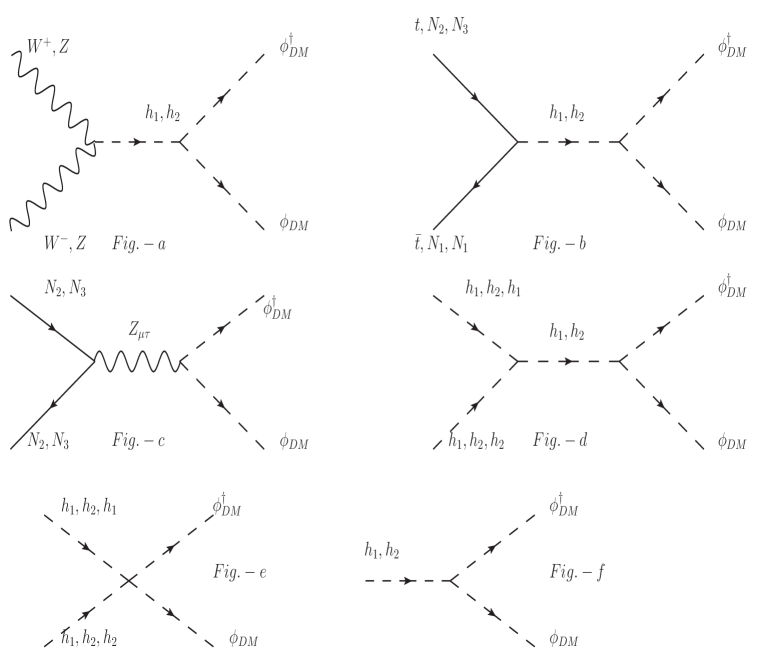
Figure 2: Feynman diagrams for the dark matter production processes from the annihilations and decays of different SM and BSM particles.

Vertex	Vertex Factor
$a\,b\,c$	$g_{abc}$
$\phi_{DM}\,\phi^{\dagger}_{DM}\,h_{1}$	$-(\lambda_{Dh}v\cos\alpha+\lambda_{DH}v_{\mu\tau}\sin\alpha)$
$\phi_{DM}\,\phi^{\dagger}_{DM}\,h_{2}$	$(\lambda_{Dh}v\sin\alpha-\lambda_{DH}v_{\mu\tau}\cos\alpha)$
$\phi_{DM}\,\phi^{\dagger}_{DM}\,Z_{\mu\tau}^{\rho}$	$n_{\mu\tau}g_{\mu\tau}(p_{2}-p_{1})^{\rho}$
$\bar{N_{i}}\,N_{i}\,Z_{\mu\tau}^{\rho}$	$\dfrac{g_{\mu\tau}}{2}\gamma^{\rho}\gamma^{5}$

Table 3: Relevant couplings required to compute Feynman diagrams given in Fig. 2.

As can be seen from the Eqs. (1–4), the dark matter particle can interact with the thermal bath containing both SM as well as BSM particles only via $h_{1}$, $h_{2}$ and $Z_{\mu\tau}$. The Feynman diagrams relevant for the production of dark matter are shown in Fig. 2. The corresponding couplings are listed in Table 3. From Table 3, one can see that the couplings of $\phi_{DM}$ with scalar bosons $h_{1}$ and $h_{2}$ depend on the parameters $\lambda_{Dh}$ and $\lambda_{DH}$, while that with extra neutral gauge boson $Z_{\mu\tau}$ involves $g_{\mu\tau}$ and $n_{\mu\tau}$. For the dark matter to be a suitable FIMP candidate, the cross section of the diagrams listed in Fig. 2 should be very small. The complete expressions for the contribution from each of the diagrams is given in Appendix A and B. The processes involving $h_{1}$ and $h_{2}$ can be easily made feeble enough by taking $\lambda_{Dh}$ and $\lambda_{DH}\sim 10^{-12}$. As we will see later, the other important production mechanism of $\phi_{DM}$ is shown by the Feynman diagram where $N_{2}$ and $N_{3}$ annihilate to $\phi_{DM}$ via the new gauge boson $Z_{\mu\tau}$. The expression for the cross section of this process is given in Eq. (45) in Appendix A. We see that the cross section for this process is proportional to $\sim g_{\mu\tau}^{4}n_{\mu\tau}^{2}/10^{2}$. Since we fix $g_{\mu\tau}=9\times 10^{-4}$ to explain the anomalous muon $(g-2)$, we take $n_{\mu\tau}\sim 10^{-5}$ to keep $\sigma_{N_{j}N_{j}\rightarrow\phi_{DM}^{\dagger}\phi_{DM}}$ small enough so that $\phi_{DM}$ stays out of chemical equilibrium. This choice for $n_{\mu\tau}$ also ensures that there is a remnant $Z_{2}$ symmetry even when ${\rm U(1)}_{L_{\mu}-L_{\tau}}$ symmetry is broken spontaneously, which enables $\phi_{DM}$ to be stable. Thus, $\phi_{DM}$ behaves as a FIMP dark matter, it stays out of thermal equilibrium at all times, and is produced by the freeze-in mechanism.

The evolution of comoving number density of FIMP produced from the decays as well as annihilations of the SM and BSM particles is governed by the Boltzmann equation. The Boltzmann equation in terms of the comoving number density of $\phi_{DM}$ is given below. This equation contains both decay as well as annihilation terms. While deriving the Boltzmann equation for the FIMP $\phi_{DM}$, we have taken all the particles except $\phi_{DM}$ in thermal equilibrium and hence their number densities follow the Maxwell-Boltzmann distribution function.

$$\dfrac{dY_{\phi_{DM}}}{dz}=\dfrac{2M_{pl}}{1.66M_{h_{2}}^{2}}\dfrac{z\sqrt{g_{\star}(z)}}{g_{s}(z)}\,\,\Bigg{[}\sum_{i=1,\,2}\langle\Gamma_{h_{i}\rightarrow}\phi_{DM}^{\dagger}\phi_{DM}\rangle(Y_{i}^{eq}-Y_{\phi_{DM}})\Bigg{]}$$

$$\leavevmode\nobreak\ \leavevmode\nobreak\ \leavevmode\nobreak\ \leavevmode\nobreak\ \leavevmode\nobreak\ \leavevmode\nobreak\ \leavevmode\nobreak\ \leavevmode\nobreak\ \leavevmode\nobreak\ +\dfrac{4\pi^{2}}{45}\dfrac{M_{pl}M_{h_{2}}}{1.66}\dfrac{\sqrt{g_{\star}(z)}}{z^{2}}\,\,\Bigg{[}\sum_{p=W,Z,h_{1},h_{2},f}\langle\sigma{\rm v}_{p\bar{p}\rightarrow\phi_{DM}^{\dagger}\phi_{DM}}\rangle(Y_{p}^{eq\,\,2}-Y_{\phi_{DM}}^{2})$$

$$\leavevmode\nobreak\ \leavevmode\nobreak\ \leavevmode\nobreak\ \leavevmode\nobreak\ \leavevmode\nobreak\ \leavevmode\nobreak\ \leavevmode\nobreak\ \leavevmode\nobreak\ \leavevmode\nobreak\ +\sum_{i=1,j=2,3}\langle\sigma{\rm v}_{N_{i}N_{j}\rightarrow\phi_{DM}^{\dagger}\phi_{DM}}\rangle(Y_{N_{i}}^{eq}Y_{N_{j}}^{eq}-Y_{\phi_{DM}}^{2})+\langle\sigma{\rm v}_{h_{1}h_{2}\rightarrow\phi_{DM}^{\dagger}\phi_{DM}}\rangle(Y_{h_{1}}^{eq}Y_{h_{2}}^{eq}-Y_{\phi_{DM}}^{2})\Bigg{]}\,.$$

(30)

In the above equation $Y_{\phi_{DM}}=\dfrac{n_{\phi_{DM}}}{\rm s}$ is the comoving number density, $n_{\phi_{DM}}$ represents the actual number density of the dark matter candidate $\phi_{DM}$ while ${\rm s}$ is the entropy of the Universe. The quantity $z=\dfrac{\Lambda}{T}$, where $\Lambda$ is some mass scale and here it corresponds to the mass of the second Higgs $h_{2}$ ($\Lambda\sim M_{h_{2}}$). The temperature of the Universe is denoted by $T$ and $M_{pl}=1.22\times 10^{19}$ GeV is the Planck mass. The function $g_{\star}(z)$ is related to the degrees of freedom and has the following expression,

$$\sqrt{g_{\star}(z)}=\dfrac{g_{\rm s}(z)}{\sqrt{g_{\rho}(z)}}\,\left(1-\dfrac{1}{3}\dfrac{{\rm d}\,{\rm ln}\,g_{\rm s}(z)}{{\rm d}\,{\rm ln}z}\right)\,.$$ (31)

In the above equation $g_{s}(z)$ and $g_{\rho}(z)$ are the effective degrees of freedom corresponding to the entropy and energy densities of the Universe. If the decaying particles ($h_{1}$, $h_{2}$) are in thermal equilibrium then the thermal average of the decay width can be expressed in a simpler form as follows,

$$\langle\Gamma_{h_{i}\rightarrow}\phi_{DM}^{\dagger}\phi_{DM}\rangle\,\,=\,\dfrac{K_{1}(z)}{K_{2}(z)}\,\,\Gamma_{i\rightarrow}\phi_{DM}^{\dagger}\phi_{DM}\,.$$ (32)

In the above expression $K_{1}(z)$ and $K_{2}(z)$ are the modified Bessel’s functions of order one and two, respectively.

Next we explain the Boltzmann equation given in Eq. (30) term by term. The first term on the R.H.S represents the contribution to $Y_{\phi_{DM}}$ arising from the decays of $h_{1}$ and $h_{2}$ and it is proportional to the equilibrium comoving number density of the decaying particle. On the other hand, the inverse decay term proportional to the comoving number density of $\phi_{DM}$ occurs with a negative sign as it washes out the $\phi_{DM}$ number density. However, as we have mentioned before that the initial number density of $\phi_{DM}$ is extremely small due to its non-thermal origin and hence the negative feedback coming from the inverse processes can be safely neglected.

Similarly, the second, third and fourth terms in the R.H.S of Eq. (30) indicate the net contribution to $Y_{\phi_{DM}}$ coming from the annihilations of SM and BSM particles at the early stage of the Universe. Unlike the first term (decay term) of Eq. (30) these terms are proportional to the second power of the comoving number densities of relevant particles. The term proportional to $Y^{2}_{p}$ ($p=W,\,Z,\,h_{1},\,h_{2},\,f$) (in the second term of the Boltzmann equation) represents the increment of $Y_{\phi_{DM}}$ from the pair annihilation of $p$ and its antiparticle while the feedback arising from the inverse process $\phi_{DM}{\phi^{\dagger}_{DM}}\rightarrow p\bar{p}$ is proportional to $Y^{2}_{\phi_{DM}}$ and comes with a negative sign. The rest of the annihilation terms represent the production processes of $\phi_{DM}$ from the annihilations of two different particles such as ($N_{i},\,N_{j}$), ($h_{1},\,h_{2}$) and consequently these terms are proportional to the comoving number densities of two different initial state particles. The terms indicating the inverse processes ($\phi_{DM}\phi_{DM}^{\dagger}\rightarrow N_{i}N_{j}$, $h_{i}h_{j}$, $i\neq j$) are proportional to $Y^{2}_{\phi_{DM}}$, as in the second term of the Boltzmann equation. All the annihilation terms of Eq. (30) are proportional to the thermal averaged annihilation cross sections of relevant processes and if all the other particles (except $\phi_{DM}$) involved in the annihilation processes are in thermal equilibrium then the general expression of thermally averaged annihilation cross section of a process $A\,B\,\,\rightarrow\phi_{DM}^{\dagger}\,\phi_{DM}$ is given by

$$f_{1} = \sqrt{s^{2}+(M_{A}^{2}-M_{B}^{2})^{2}-2\,s\,(M_{A}^{2}+M_{B}^{2})}\,,$$

$$f_{2} = \sqrt{s-(M_{A}-M_{B})^{2}}\,\,\sqrt{s-(M_{A}+M_{B})^{2}}\,\,,$$

$$\langle\sigma v_{A\,B\rightarrow\phi_{DM}^{\dagger}\phi_{DM}}\rangle = \dfrac{1}{8\,M_{A}^{2}\,M_{B}^{2}\,T\,K_{2}\left(\dfrac{M_{A}}{T}\right)\,K_{2}\left(\dfrac{M_{B}}{T}\right)}\times$$ (33)

$$\int_{(M_{A}+M_{B})^{2}}^{\infty}\dfrac{\sigma_{A\,B\rightarrow}\phi_{DM}^{\dagger}\phi_{DM}}{\sqrt{s}}\,f_{1}\,f_{2}\,K_{1}\left(\dfrac{\sqrt{s}}{T}\right)\,{\rm d}s\,.$$

In the above Eq. (33), $s$ is the Mandelstam variable, $M_{A}$ and $M_{B}$ are the masses of the initial state particles, $\sigma_{A\,B\rightarrow}\phi_{DM}^{\dagger}\phi_{DM}$ is the annihilation cross section, while $K_{i}(x)$ is the modified Bessel function of order $i$. In order to get the comoving number density ($Y_{\phi_{DM}}$) of the DM particle $\phi_{DM}$, we have to solve the Boltzmann equation numerically. After determining the comoving number density $Y_{\phi_{DM}}$ of dark matter particle $\phi_{DM}$ at the present epoch, we can determine the relic density Edsjo:1997bg ; Biswas:2011td from the following relation,

$$\Omega_{\phi_{DM}}h^{2}=2.755\times 10^{8}\,\left(\dfrac{M_{\phi_{DM}}}{\rm GeV}\right)\,Y_{\phi_{DM}}(T_{0})\,,$$ (34)

where $M_{DM}$ is in GeV. The observed value of the dark matter relic density given by the Planck collaboration Ade:2015xua , is

$$\Omega_{\phi_{DM}}h^{2}=0.1197\pm 0.0022.$$ (35)

In this work we have used the above relic density bound.

V Results

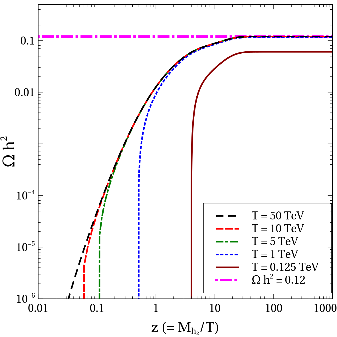
Figure 3: Variation of relic density for different choices of initial temperature while the other parameters have been kept fixed at, $M_{Z_{\mu\tau}}=0.1$ GeV, $g_{\mu\tau}=9.0\times 10^{-4}$, $\alpha=0.01$, $\lambda_{Dh}=9.8\times 10^{-13}$, $\lambda_{DH}=1.3\times 10^{-11}$, $M_{DM}=50.0$ GeV, $n_{\mu\tau}=5.5\times 10^{-5}$.

We have implemented our model in LanHEP Semenov:2010qt to generate all the vertex factors which are required to calculate the relevant annihilation cross sections and decay widths. Corresponding Feynman diagrams are shown in Fig. 2. After putting all the cross sections and decay widths (as listed in Appendix A and Appendix B) in Eq. (30), we solve the Boltzmann equation numerically and study the related phenomenology of FIMP dark matter. Throughout this analysis we keep the extra Higgs mass fixed at $M_{h_{2}}=500$ GeV. In Fig. 3, we show the variation of the dark matter relic density with $z$ for different choices of the initial temperature. From the figure, it is clear that if the initial temperature is greater $T_{\rm in}\geq 1$ TeV, then there is no dependence of the final relic density on the value of the initial temperature. This can be explained in the following way. As the heavy Higgs $h_{2}$ is in thermal equilibrium with the cosmic soup, hence the maximum production of $\phi_{DM}$ from the decay of $h_{2}$ occurs around a temperature of the Universe ($T$) $\sim M_{h_{2}}$ i.e. 500 GeV. However, as the temperature of the Universe drops below $M_{h_{2}}$, the number density of the extra Higgs boson ($h_{2}$) becomes exponentially suppressed (or Boltzmann suppressed), which in turn reduces the final abundance of $\phi_{DM}$. This case is shown by the choice $T_{\rm in}=125\,\,\text{GeV}$ in the figure. Hence in what follows, we take a fixed $T_{\rm in}=1\,\,{\rm TeV}$.

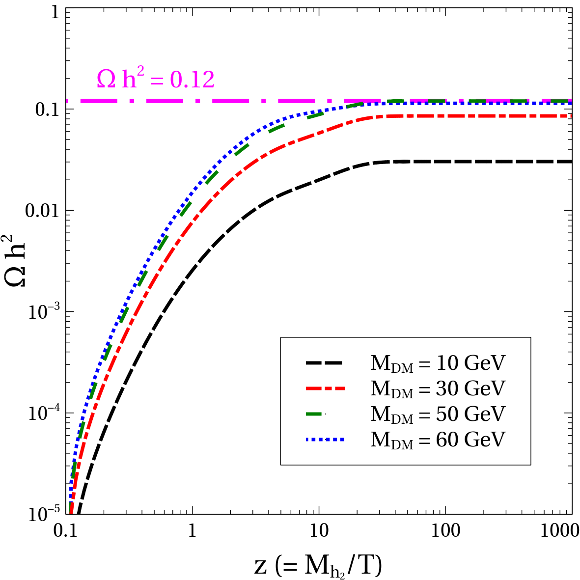
Figure 4: Left panel showing the contributions of decay and annihilation in the total relic density. Right panel: Variation of dark matter relic density with $z$ for four different values of dark matter mass M_DM. The other parameters are kept fixed at $M_{Z_{\mu\tau}}=0.1$ GeV, $g_{\mu\tau}=9.0\times 10^{-4}$, $\alpha=0.01$, $\lambda_{Dh}=9.8\times 10^{-13}$, $\lambda_{DH}=1.3\times 10^{-11}$, $M_{DM}=50.0$ GeV (LP), $n_{\mu\tau}=5.5\times 10^{-5}$.

In the left panel of Fig. 4, we show the relative contributions of two different types of production processes (decay and annihilation) to $\Omega h^{2}$. The red dotted line represents the contribution from the decay of SM-like Higgs boson h₁ and extra Higgs boson h₂, while the black dashed line corresponds to the contribution from the all possible annihilation channels of SM and BSM particles (see Fig. 2 for the corresponding Feynman diagrams). The total contribution towards the relic density of $\phi_{DM}$ coming from the decay as well as annihilation of different particles is represented by blue dashed-dotted line. The horizontal magenta line indicates the observed value of dark matter relic density ($\Omega h^{2}\sim 0.12$ Ade:2015xua ) at the present epoch. From this plot, it can be seen clearly that for our chosen set of model parameters ($M_{Z_{\mu\tau}}=0.1$ GeV, $g_{\mu\tau}=9.0\times 10^{-4}$, $\alpha=0.01$, $\lambda_{Dh}=9.8\times 10^{-13}$, $\lambda_{DH}=1.3\times 10^{-11}$, $M_{DM}=50.0$ GeV, $n_{\mu\tau}=5.5\times 10^{-5}$), the decay processes contribute $\sim 67\%$ of dark matter production while rest of the dark matter particles are produced from the annihilations of different SM as well as BSM particles. In the right panel of Fig. 4, the variation of relic density with $z$ (i.e. with respect to the inverse of temperature $T$) has been shown for four different values of dark matter mass $M_{DM}$. For M${}_{DM}=$ 10 GeV, 30 GeV and 50 GeV, the relic density is seen to rise with M_DM. This agrees with the expression for relic density given in Eq. (34). However, if we take a slightly higher value of dark matter mass, M${}_{DM}=$ 60 GeV (blue dotted line), the relic density decreases instead of increasing. This is because M${}_{DM}=$ 60 GeV is very close to half of the SM like Higgs boson mass ($\sim M_{h_{1}}/2$) and the decay mode $h_{1}\rightarrow\phi_{DM}\phi_{DM}^{\dagger}$ becomes phase space suppressed. Therefore, it reduces the contribution arising from $h_{1}$ decay and hence the final relic density of dark matter.

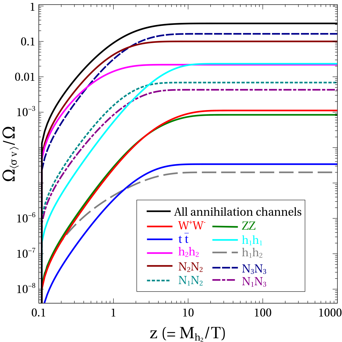
Figure 5: Left Panel: Relative contributions of two decay modes in relic density. Right Panel: Relative contributions of different annihilation channels towards $\Omega h^{2}$. Other parameters are kept fixed at $M_{Z_{\mu\tau}}=0.1$ GeV, $g_{\mu\tau}=9.0\times 10^{-4}$, $\alpha=0.01$, $\lambda_{Dh}=9.8\times 10^{-13}$, $\lambda_{DH}=1.3\times 10^{-11}$, $M_{DM}=50.0$ GeV, $n_{\mu\tau}=5.5\times 10^{-5}$.

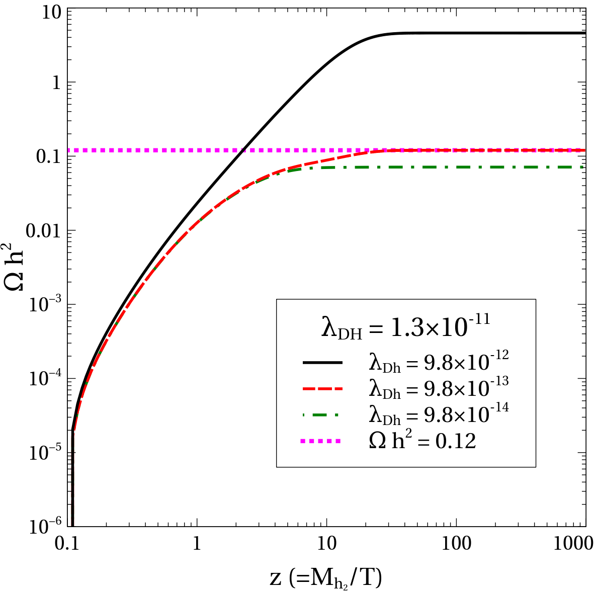
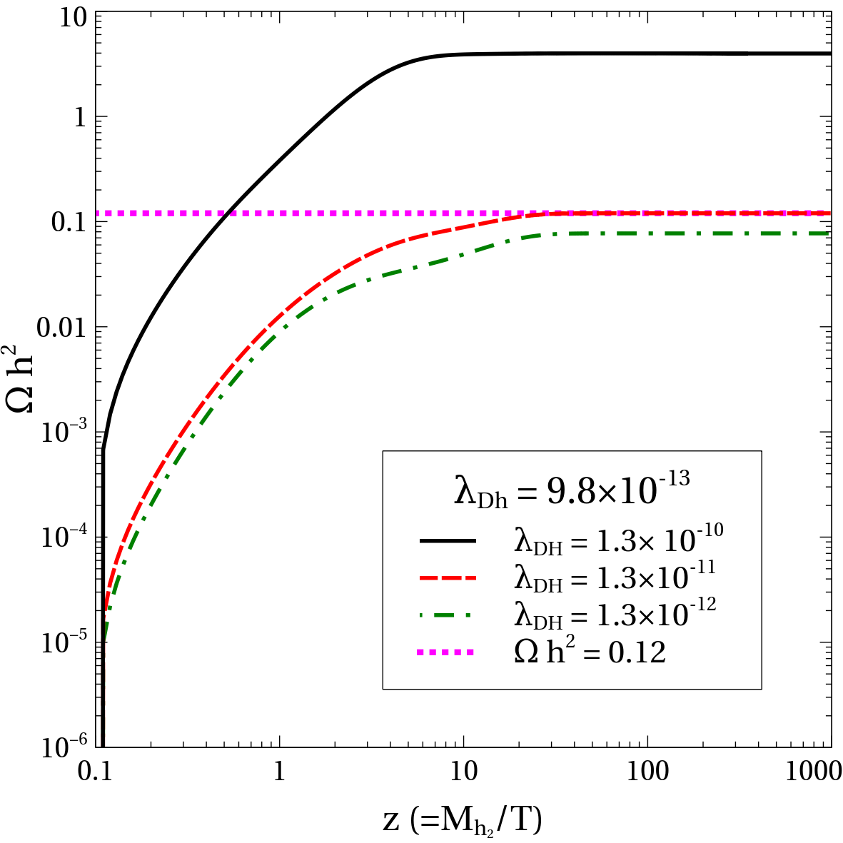
Figure 6: Left (Right) Panel: Variation of relic density with $z$ for three different values of $\lambda_{Dh}$ ($\lambda_{DH}$). Other parameters are kept fixed at $M_{Z_{\mu\tau}}=0.1$ GeV, $g_{\mu\tau}=9.0\times 10^{-4}$, $\alpha=0.01$, $\lambda_{Dh}=9.8\times 10^{-13}$, $\lambda_{DH}=1.3\times 10^{-11}$, $M_{DM}=50.0$ GeV, $n_{\mu\tau}=5.5\times 10^{-5}$.

The contributions to $\Omega h^{2}$ arising from the decays of $h_{1}$, $h_{2}$ and the annihilations of SM as well as BSM particles are shown respectively in left and right panels of Fig. 5. Here we define a quantity $\frac{\Omega_{\langle\Gamma\rangle}}{\Omega}$ ($\frac{\Omega_{\langle\sigma{\rm v}\rangle}}{\Omega}$) which represents the fractional contribution of a particular decay (annihilation) channel to dark matter relic density. In the left-panel of Fig. 5, the contribution from h₂ decay has been shown by the green dashed-dotted line and that from h₁ decay has been shown by the red dashed line, while the total decay contribution to the dark matter relic density is represented by the black solid line. From this plot one can see that, initially for low values of $z$ ($z<10$, corresponding to higher temperatures), the extra Higgs contribution to $\Omega h^{2}$ is more because of its high mass. On the other hand, for higher values of $z$ ($z>10$), the SM-like Higgs decay contribution starts dominating. In the right panel of Fig. 5, we show the contribution coming from different annihilation channels. The total contribution from all the annihilation channels is represented by the black solid line while the other lines show the contribution of individual channels. From this plot it is clearly seen that, the two dominating annihilation channels are $N_{2}\,N_{2}$ and $N_{3}\,N_{3}$. Annihilation channels $h_{1}\,h_{1}$ and $h_{2}\,h_{2}$ also have significant role in the production processes of dark matter, while the effect of other channels are sub dominant. In the left-panel of Fig. 6, variation of relic density with $z$ for three different value of $\lambda_{Dh}$ have been shown. The red dashed line for $\lambda_{Dh}=9.8\times 10^{-13}$ gives the correct relic density. In the right-panel of Fig. 6 we show the variation of relic density for different values of the other quartic coupling $\lambda_{DH}$. It is clear from Fig. 6 that the relic density increases with both $\lambda_{Dh}$ and $\lambda_{DH}$ as the production modes of $\phi_{DM}$ are proportional to these quartic couplings. However, the increment of $\Omega h^{2}$ with respect to increasing $\lambda_{Dh}$ or $\lambda_{DH}$ is not uniform. When we decrease $\lambda_{Dh}$ ($\lambda_{DH}$) from $9.8\times 10^{-13}$ ($1.3\times 10^{-11}$) by one order of magnitude, the decrease in $\Omega h^{2}$ is very small because in this regime we have dominant contribution from the $Z_{\mu\tau}$ mediated right-handed neutrino annihilation channel. However, if we increase $\lambda_{Dh}$ ($\lambda_{DH}$) from $9.8\times 10^{-13}$ ($1.3\times 10^{-11}$) by one order of magnitude, $\Omega h^{2}$ increases by more than order of magnitude since in this case the contribution from decay channels become dominant.

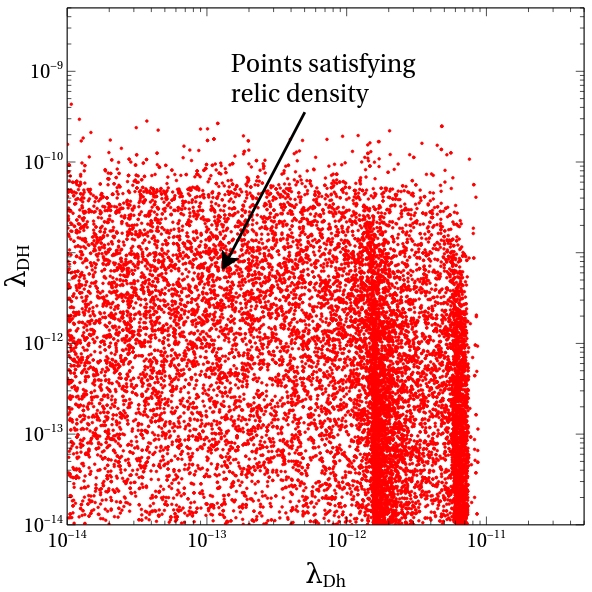
Figure 7: Left panel: Allowed parameter space in $\lambda_{Dh}$ - $\lambda_{DH}$ plane. Right panel: Allowed parameter space in $M_{DM}$ - $g_{\mu\tau}$ plane. In both the plots red points satisfy the relic density bound.

In the left-panel of Fig. 7, we have shown the allowed regions in the $\lambda_{Dh}$ - $\lambda_{DH}$ plane. The red points in the plane satisfy the relic density bound. Both the parameters $\lambda_{Dh}$ and $\lambda_{DH}$ have been varied from 10^-14 to 10^-8. We see from the figure that for $\lambda_{Dh}\geq 8\times 10^{-11}$ and $\lambda_{Dh}\geq 3\times 10^{-10}$ no red points exist, and therefore these regions are disallowed by the relic density bound. One can also notice that there is no lower bound on $\lambda_{Dh}$ and $\lambda_{DH}$. This is because for lower values of $\lambda_{Dh}$ and $\lambda_{DH}$, even though the Higgs mediated annihilation and decay contributions become very less, the $Z_{\mu\tau}$ mediated annihilation channels ($N_{i}\,{N_{i}}\rightarrow\phi_{DM}^{\dagger}\,\phi_{DM}$, $i=2,3$ see Appendix A) contribute fully and hence can explain the relic density bound. In the right-panel of Fig. 7, we show the allowed regions in the $M_{DM}$ - $g_{\mu\tau}$ plane. Here we have varied dark matter mass $M_{DM}$ from 1 GeV to 100 GeV and the ${\rm U(1)}_{L_{\mu}-L_{\tau}}$ gauge coupling $g_{\mu\tau}$ from 10^-6 to 0.1. The figure shows that the whole range of dark matter mass $M_{DM}$ can satisfy the relic density bound. However, the gauge coupling $g_{\mu\tau}\geq 3\times 10^{-3}$ does not satisfy the relic density bound as over production of $\phi_{DM}$ occurs through the annihilation channel $N_{i}\,{N_{i}}\rightarrow\phi_{DM}^{\dagger}\,\phi_{DM}$, $i=2,3$.

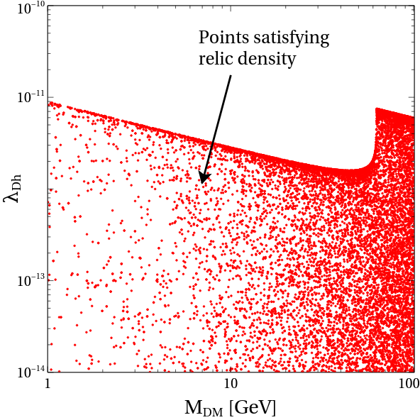
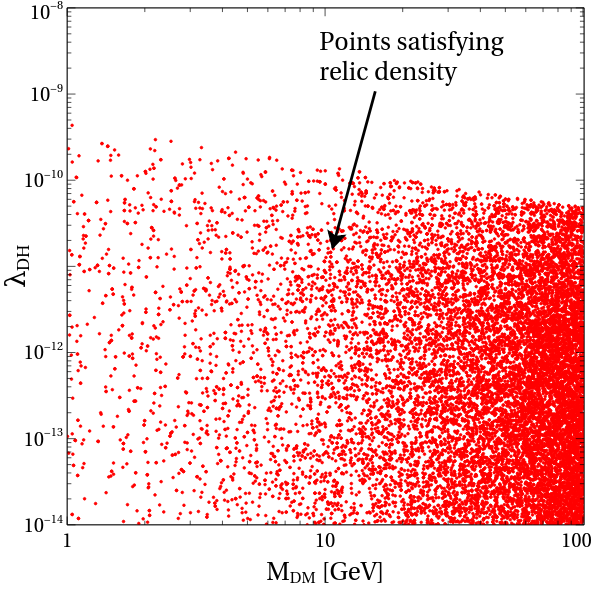
Figure 8: Left panel: Allowed parameter space in $M_{DM}$ - $\lambda_{Dh}$ plane. Right panel: Allowed parameter space in $M_{DM}$ - $\lambda_{DH}$ space. In both the plots red points satisfy the relic density bound.

In Fig. 8, we show the allowed parameter space in the $M_{DM}-\lambda_{Dh}$ and $M_{DM}-\lambda_{DH}$ planes in the left and right panels respectively. As it was seen earlier, here too the whole range of considered dark matter mass is allowed. However, there is an upper limit on both $\lambda_{Dh}$ and $\lambda_{DH}$. In both the panels, there exist an anti-correlation between the dark matter mass and the quartic coupling $\lambda_{Dh(H)}$ since the relic density is proportional to the dark matter mass $M_{DM}$ as well as the coupling constant. Hence, if we increase $M_{DM}$ then to satisfy the relic density, $\lambda_{Dh(H)}$ must decrease. In the left-panel we observe that around $M_{DM}\sim 62$ GeV, there is a rise in $\lambda_{Dh}$. This happens because this is the resonance region for the SM-like Higgs and as a result there is little contribution from the decay of SM-like Higgs (phase space suppression). Hence, to satisfy the relic density bound, there is a sudden rise in $\lambda_{Dh}$ to increase the contribution arising from the decay as well as annihilation processes involving $h_{1}$. Beyond $M_{DM}\sim 62.5$ GeV, there is no contribution from the SM-like Higgs. Hence, the coupling $\lambda_{Dh}$ again starts behaving in the normal way (anti-correlation). No such peculiar behaviour is seen for $\lambda_{DH}$ because this parameter is important for the decay of $h_{2}$ and the chosen mass range of the dark matter is not in the resonance region of the extra Higgs $h_{2}$ ($M_{h_{2}}\sim$ 500 GeV). Therefore, for the quartic coupling $\lambda_{DH}$, the anti-correlation exists for the entire range of dark matter mass $M_{DM}$ (1-100 GeV).

VI Conclusion

In this work, we propose a framework for non-thermal production of a FIMP type dark matter in the gauged U(1)${}_{L_{\mu}-L_{\tau}}$ extension of the SM. The particle content of our model includes two SM gauge singlet scalars and three right-handed neutrinos. Both the SM singlet scalars carry U(1)${}_{L_{\mu}-L_{\tau}}$ charge. One of them picks up a VEV, breaking U(1)${}_{L_{\mu}-L_{\tau}}$ spontaneously, thereby giving the new gauge boson $Z_{\mu\tau}$ mass. The new boson $Z_{\mu\tau}$ gives additional contribution to muon $(g-2)$ which can explain its measured value. The U(1)${}_{L_{\mu}-L_{\tau}}$ breaking also leads to additional terms in the light neutrino mass matrix which has its origin via the Type-I seesaw mechanism. This model can therefore explain consistently the neutrino masses and mixing patterns observed in neutrino oscillation experiments. Finally, the other SM singlet scalar $\phi_{DM}$ does not acquire any VEV and remains stable due to a remnant $Z_{2}$ symmetry even after the breaking of U(1)${}_{L_{\mu}-L_{\tau}}$ due to our choice of its $L_{\mu}-L_{\tau}$ charge ($n_{\mu\tau}$). This scalar can therefore serve as a dark matter candidate.

In this model, $\phi_{DM}$ can interact with the visible sector (including both SM as well as BSM particles) only through the scalar bosons $h_{1}$, $h_{2}$ and $L_{\mu}-L_{\tau}$ gauge boson $Z_{\mu\tau}$. Hence, in order to keep $\phi_{DM}$ out of thermal equilibrium we have considered the corresponding couplings of $\phi_{DM}$ to be extremely feeble. All other particles (both SM and BSM) in the early Universe, however remain in equilibrium with the thermal soup. We have numerically solved the Boltzmann equation containing all possible production modes of $\phi_{DM}$ from decays and annihilations of SM and BSM particles. We have found that, among all of its production modes, $\phi_{DM}$ is mainly produced from the decays of $h_{1}$, $h_{2}$ and the pair annihilations of right handed neutrinos mediated by $Z_{\mu\tau}$. The latter process beautifully sets the interplay between the dark matter sector, neutrino masses and muon $(g-2)$. The solution of Boltzmann equation also indicates that, for our chosen set of model parameters, decay processes of $h_{1}$ and $h_{2}$ contribute $\sim 67\%$ of the total dark matter relic abundance while rest $\sim 33\%$ contribution is coming from the annihilation of particles (mainly right-handed neutrinos) in the thermal bath. We have shown that, the relic abundance of our FIMP type dark matter candidate $\phi_{DM}$ lies within the Planck Limit (0.1172 $\leq\Omega h^{2}\leq 0.1224$) only when the relevant parameters satisfy the following bounds: $\lambda_{Dh}\mathrel{\mathchoice{\vbox{\offinterlineskip\halign{\hfil$\displaystyle#$\hfil\cr<\cr\sim\cr}}}{\vbox{\offinterlineskip\halign{\hfil$\textstyle#$\hfil\cr<\cr\sim\cr}}}{\vbox{\offinterlineskip\halign{\hfil$\scriptstyle#$\hfil\cr<\cr\sim\cr}}}{\vbox{\offinterlineskip\halign{\hfil$\scriptscriptstyle#$\hfil\cr<\cr\sim\cr}}}}10^{-11}$, $\lambda_{DH}\mathrel{\mathchoice{\vbox{\offinterlineskip\halign{\hfil$\displaystyle#$\hfil\cr<\cr\sim\cr}}}{\vbox{\offinterlineskip\halign{\hfil$\textstyle#$\hfil\cr<\cr\sim\cr}}}{\vbox{\offinterlineskip\halign{\hfil$\scriptstyle#$\hfil\cr<\cr\sim\cr}}}{\vbox{\offinterlineskip\halign{\hfil$\scriptscriptstyle#$\hfil\cr<\cr\sim\cr}}}}10^{-10}$ and $g_{\mu\tau}\leq 3\times 10^{-3}$ for the dark matter mass range of 1 GeV to 100 GeV and $n_{\mu\tau}=5.5\times 10^{-5}$. Consequently, due to the low coupling strength there does not exist any bound on dark matter spin independent scattering cross section from direct detection experiments.

In conclusion, our proposed U(1)${}_{L_{\mu}-L_{\tau}}$ extension of the SM can explain the three main puzzles that demand beyond Standard Model physics. First, it can successfully explain the smallness of neutrino masses via the Type-I seesaw mechanism as well as the peculiar mixing pattern of the neutrinos via the U(1)${}_{L_{\mu}-L_{\tau}}$ gauge symmetry that also acts on the lepton flavours, thereby giving a pattern to the light neutrino mass matrix. Second, the additional one loop contribution of the extra neutral gauge boson $Z_{\mu\tau}$ can successfully satisfy the muon ($g-2$) data. And finally, the model has a SM singlet scalar with non-zero U(1)${}_{L_{\mu}-L_{\tau}}$, that makes it stable and which acts as a non-thermal dark matter candidate, thereby satisfying constraint on the relic abundance and at the same time evading all bounds coming from direct and indirect dark matter detection experiments.

VII Acknowledgements

The authors would like to thank the Department of Atomic Energy (DAE) Neutrino Project under the XII plan of Harish-Chandra Research Institute. SK and AB also acknowledge the cluster computing facility at HRI (http://cluster.hri.res.in). This project has received funding from the European Union’s Horizon 2020 research and innovation programme InvisiblesPlus RISE under the Marie Sklodowska-Curie grant agreement No 690575. This project has received funding from the European Union’s Horizon 2020 research and innovation programme Elusives ITN under the Marie Sklodowska- Curie grant agreement No 674896.

Appendix

Appendix A Analytical Expression of relevant Cross sections

In this section we have given all the relevant cross sections which are required to solve the Boltzmann equation (Eq. (30)) numerically. We have expressed all the cross sections in terms of three Mandelstam variables. Here, we have used the usual particle notation as we have given in the model section. The vertex factors which are common to the most of the annihilation diagrams are,

$$g_{h_{1}\phi_{DM}\phi_{DM}} = -\left(v\lambda_{Dh}\cos\alpha+v_{\mu\tau}\lambda_{DH}\sin\alpha\right)\,,$$

$$g_{h_{2}\phi_{DM}\phi_{DM}} = \left(v\lambda_{Dh}\sin\alpha-v_{\mu\tau}\lambda_{DH}\cos\alpha\right)\,.$$ (36)

• $W^{+}$ $W^{-}$ $\rightarrow\phi_{DM}^{\dagger}\,\phi_{DM}$ :
  
  The annihilation of the vector bosons $W^{+}$ and $W^{-}$ into the dark matter $\phi_{DM}$ and $\phi_{DM}^{\dagger}$ are occurred by the two s channel diagrams which are mediated by the SM-like Higgs $h_{1}$ and the SM extra Higgs boson $h_{2}$. Expression of this annihilation cross section is,

  $$g_{h_{1}WW} = \dfrac{2M_{W}^{2}\cos\alpha}{v}\,,$$

  $$g_{h_{2}WW} = -\dfrac{2M_{W}^{2}\sin\alpha}{v},$$

  $$A_{WW} = \dfrac{g_{h_{1}WW}\,\,g_{h_{1}\phi_{DM}^{\dagger}\phi_{DM}}}{(s-M_{h_{1}}^{2})+iM_{h_{1}}\Gamma_{h_{1}}}+\dfrac{g_{h_{2}WW}\,g_{h_{2}\phi_{DM}^{\dagger}\phi_{DM}}}{(s-M_{h_{2}}^{2})+iM_{h_{2}}\Gamma_{h_{2}}},$$

  $$M_{WW} = \dfrac{2}{9}\,\left(1+\dfrac{(s-2M_{W}^{2})^{2}}{8M_{W}^{4}}\right)\,A_{WW},$$

  $$\sigma_{WW\rightarrow\phi_{DM}^{\dagger}\phi_{DM}} = \dfrac{1}{16\pi s}\,\,\sqrt{\dfrac{s-4M_{DM}^{2}}{s-4M_{W}^{2}}}\,\,\,|M_{WW}|^{2}\,.$$ (37)

  where $|M_{WW}|^{2}$ represents the square of the absolute value of $M_{WW}$. The couplings $g_{h_{1}\phi_{DM}^{\dagger}\phi_{DM}}$ and $g_{h_{2}\phi_{DM}^{\dagger}\phi_{DM}}$ are given in Eq. (36) while $\Gamma_{h_{1}}$ and $\Gamma_{h_{2}}$ are the total decay widths of the SM-like Higgs and the extra Higgs respectively (see Appendix B for more details). In the expression of $M_{WW}$ the extra factor 1/9 comes due to average of the polarisation vectors of two initial state $W$ bosons.

• $Z\,Z\rightarrow\phi_{DM}^{\dagger}\,\phi_{DM}$ :
  
  The self annihilation of $Z$ boson to dark matter particles $\phi_{DM}$ and $\phi_{DM}^{\dagger}$ has two $s$ channel diagrams, one of them is mediated by the SM-like Higgs $h_{1}$ while another one is mediated by the extra Higgs $h_{2}$. Cross section structure for the $Z\,Z$ annihilation is similar to $W^{+}\,W^{-}$ annihilation and has the following form,

  $$g_{h_{1}ZZ} = \dfrac{2M_{Z}^{2}\cos\alpha}{v}\,,$$

  $$g_{h_{2}ZZ} = -\dfrac{2M_{Z}^{2}\sin\alpha}{v},$$

  $$A_{ZZ} = \dfrac{g_{h_{1}ZZ}\,g_{h_{1}\phi_{DM}^{\dagger}\phi_{DM}}}{(s-M_{h_{1}}^{2})+iM_{h_{1}}\Gamma_{h_{1}}}+\dfrac{g_{h_{2}ZZ}\,g_{h_{2}\phi_{DM}^{\dagger}\phi_{DM}}}{(s-M_{h_{2}}^{2})+iM_{h_{2}}\Gamma_{h_{2}}},$$

  $$M_{ZZ} = \dfrac{2}{9}\,\,\left(1+\dfrac{(s-2M_{Z}^{2})^{2}}{8M_{Z}^{4}}\right)\,A_{ZZ},$$

  $$\sigma_{ZZ\rightarrow\phi_{DM}^{\dagger}\phi_{DM}} = \dfrac{1}{16\pi s}\,\,\sqrt{\dfrac{s-4M_{DM}^{2}}{s-4M_{Z}^{2}}}\,\,\,|M_{ZZ}|^{2}\,.$$ (38)

• $h_{1}$ $h_{1}$ $\rightarrow\phi_{DM}^{\dagger}\,\phi_{DM}$ :
  
  The annihilation of two $h_{1}$ to $\phi_{DM}^{\dagger}\,\phi_{DM}$ occurs through one four points interaction process as well as two $s$ channel processes mediated by the SM-like Higgs $h_{1}$ and extra Higgs $h_{2}$. The expression of the cross section is the following,

  $$g_{h_{1}h_{1}h_{1}}=-3\,[2\,v\lambda_{h_{1}}\cos^{3}\alpha+2\,v_{\mu\tau}\,\lambda_{h_{2}}\sin^{3}\alpha+\lambda_{h_{1}h_{2}}\sin\alpha\,\cos\alpha\,(v\sin\alpha+v_{\mu\tau}\cos\alpha)],$$

  $$g_{h_{1}h_{1}h_{2}}=[6\,v\lambda_{h_{1}}\cos^{2}\alpha\sin\alpha-6\,v_{\mu\tau}\lambda_{h_{2}}\sin^{2}\alpha\,\cos\alpha-(2-3\,\sin^{2}\alpha)\,v\,\lambda_{h_{1}h_{2}}\,\sin\alpha$$

  $$\leavevmode\nobreak\ \leavevmode\nobreak\ \leavevmode\nobreak\ \leavevmode\nobreak\ \leavevmode\nobreak\ \leavevmode\nobreak\ \leavevmode\nobreak\ \leavevmode\nobreak\ \leavevmode\nobreak\ -(1-3\sin^{2}\alpha)v_{\mu\tau}\,\lambda_{h_{1}h_{2}}\cos\alpha]\,,$$ (39)

  $$g_{h_{1}h_{1}\phi_{DM}^{\dagger}\phi_{DM}}=-(\lambda_{Dh}\cos^{2}\alpha+\lambda_{DH}\sin^{2}\alpha)\,,$$

  $$M_{h_{1}h_{1}}=\dfrac{g_{h_{1}h_{1}h_{1}}\,\,g_{h_{1}\phi_{DM}^{\dagger}\phi_{DM}}}{(s-M_{h_{1}}^{2})+iM_{h_{1}}\Gamma_{h_{1}}}+\dfrac{g_{h_{1}h_{1}h_{2}}\,\,g_{h_{2}\phi_{DM}^{\dagger}\phi_{DM}}}{(s-M_{h_{2}}^{2})+iM_{h_{2}}\Gamma_{h_{2}}}-g_{h_{1}h_{1}\phi_{DM}^{\dagger}\phi_{DM}},$$

  $$\sigma_{h_{1}h_{1}\rightarrow\phi_{DM}^{\dagger}\phi_{DM}}=\dfrac{1}{16\pi s}\,\,\sqrt{\dfrac{s-4M_{DM}^{2}}{s-4M_{h_{1}}^{2}}}\,\,\,|M_{h_{1}h_{1}}|^{2}\,.$$ (40)

• $h_{2}$ $h_{2}$ $\rightarrow\phi_{DM}^{\dagger}\,\phi_{DM}$ :
  
  Similarly, the annihilation of two $h_{2}$ to $\phi_{DM}^{\dagger}\,\phi_{DM}$ also occurs through one four points interaction process as well as two $s$ channel processes mediated by the SM like Higgs $h_{1}$ and extra Higgs $h_{2}$. The expression of annihilation cross section for $h_{2}$ $h_{2}$ $\rightarrow\phi_{DM}^{\dagger}\,\phi_{DM}$ is given by

  $$g_{h_{2}h_{2}h_{2}}=3\,[2\,v\lambda_{h_{1}}\sin^{3}\alpha-2\,v_{\mu\tau}\lambda_{h_{2}}\cos^{3}\alpha+\lambda_{h_{1}h_{2}}\sin\alpha\cos\alpha\,(v\cos\alpha-v_{\mu\tau}\sin\alpha)],$$

  $$g_{h_{2}h_{2}h_{1}}=-[6\,v\lambda_{h_{1}}\sin^{2}\alpha\cos\alpha+6\,v_{\mu\tau}\lambda_{h_{2}}\cos^{2}\alpha\sin\alpha-(2-3\,\sin^{2}\alpha)v_{\mu\tau}\lambda_{h_{1}h_{2}}\sin\alpha\,\,$$

  $$\leavevmode\nobreak\ \leavevmode\nobreak\ \leavevmode\nobreak\ \leavevmode\nobreak\ \leavevmode\nobreak\ \leavevmode\nobreak\ \leavevmode\nobreak\ \leavevmode\nobreak\ \leavevmode\nobreak\ +(1-3\sin^{2}\alpha)v\lambda_{h_{1}h_{2}}\cos\alpha]\,,$$

  $$g_{h_{2}h_{2}\phi_{DM}^{\dagger}\phi_{DM}}=-(\lambda_{Dh}\sin^{2}\alpha+\lambda_{DH}\cos^{2}\alpha)\,,$$

  $$M_{h_{2}h_{2}}=\dfrac{g_{h_{2}h_{2}h_{1}}\,\,g_{h_{1}\phi_{DM}^{\dagger}\phi_{DM}}}{(s-M_{h_{1}}^{2})+iM_{h_{1}}\Gamma_{h_{1}}}+\dfrac{g_{h_{2}h_{2}h_{2}}\,\,g_{h_{2}\phi_{DM}^{\dagger}\phi_{DM}}}{(s-M_{h_{2}}^{2})+iM_{h_{2}}\Gamma_{h_{2}}}-g_{h_{2}h_{2}\phi_{DM}^{\dagger}\phi_{DM}},$$

  $$\sigma_{h_{2}h_{2}\rightarrow\phi_{DM}^{\dagger}\phi_{DM}}=\dfrac{1}{16\pi s}\,\,\sqrt{\dfrac{s-4M_{DM}^{2}}{s-4M_{h_{2}}^{2}}}\,\,\,|M_{h_{2}h_{2}}|^{2}\,.$$ (41)

  
  

• $h_{1}$ $h_{2}$ $\rightarrow\phi_{DM}^{\dagger}\,\phi_{DM}$ :
  
  Like the previous two cases, here we also have three processes (one four points interaction and two $s$ channels) contributing to the annihilation of $h_{1}$ $h_{2}$ $\rightarrow\phi_{DM}^{\dagger}\,\phi_{DM}$. The expression of $h_{1}$ $h_{2}$ $\rightarrow\phi_{DM}^{\dagger}\,\phi_{DM}$ has the following form

  $$g_{h_{1}h_{1}h_{2}}=[6\,v\lambda_{h_{1}}\cos^{2}\alpha\,\sin\alpha-6\,v_{\mu\tau}\,\lambda_{h_{2}}\sin^{2}\alpha\,\cos\alpha-(2-3\,\sin^{2}\alpha)\,v\,\lambda_{h_{1}h_{2}}\sin\alpha$$

  $$\leavevmode\nobreak\ \leavevmode\nobreak\ \leavevmode\nobreak\ \leavevmode\nobreak\ \leavevmode\nobreak\ \leavevmode\nobreak\ \leavevmode\nobreak\ \leavevmode\nobreak\ \leavevmode\nobreak\ -(1-3\sin^{2}\alpha)v_{\mu\tau}\,\lambda_{h_{1}h_{2}}\cos\alpha]$$

  $$g_{h_{2}h_{2}h_{1}}=-[6\,v\lambda_{h_{1}}\sin^{2}\alpha\,\cos\alpha+6\,v_{\mu\tau}\lambda_{h_{2}}\cos^{2}\alpha\sin\alpha-(2-3\,\sin^{2}\alpha)\,v_{\mu\tau}\,\lambda_{h_{1}h_{2}}\sin\alpha$$

  $$\leavevmode\nobreak\ \leavevmode\nobreak\ \leavevmode\nobreak\ \leavevmode\nobreak\ \leavevmode\nobreak\ \leavevmode\nobreak\ \leavevmode\nobreak\ \leavevmode\nobreak\ \leavevmode\nobreak\ +(1-3\sin^{2}\alpha)v\lambda_{h_{1}h_{2}}\cos\alpha]\,,$$

  $$g_{h_{1}h_{2}\phi_{DM}^{\dagger}\phi_{DM}}=\sin\alpha\cos\alpha(\lambda_{Dh}-\lambda_{DH})\,,$$

  $$M_{h_{1}h_{2}}=\dfrac{g_{h_{1}h_{1}h_{2}}\,\,g_{h_{1}\phi_{DM}^{\dagger}\phi_{DM}}}{(s-M_{h_{1}}^{2})+iM_{h_{1}}\Gamma_{h_{1}}}+\dfrac{g_{h_{2}h_{2}h_{1}}\,\,g_{h_{2}\phi_{DM}^{\dagger}\phi_{DM}}}{(s-M_{h_{2}}^{2})+iM_{h_{2}}\Gamma_{h_{2}}}-g_{h_{1}h_{2}\phi_{DM}^{\dagger}\phi_{DM}},$$

  $$\sigma_{h_{1}h_{2}\rightarrow\phi_{DM}^{\dagger}\phi_{DM}}=\dfrac{1}{16\pi s}\,\,\sqrt{\dfrac{s(s-4M_{DM}^{2})}{(s-(M_{h_{1}}+M_{h_{2}})^{2})(s-(M_{h_{2}}-M_{h_{1}})^{2})}}\,\,\,|M_{h_{1}h_{2}}|^{2}\,.$$ (42)

• $t\bar{t}$  $\rightarrow\phi_{DM}^{\dagger}\,\phi_{DM}$ :
  
  Here, the annihilating particles are $t$,  $\bar{t}$ and the final particles are $\phi_{DM}$,  $\phi_{DM}^{\dagger}$. This annihilation is occurred only by the two $s$ channel diagrams mediated via $h_{1}$ and $h_{2}$ respectively. The expression of the cross section for this process is,

  $$g_{h_{1}tt} = -\dfrac{M_{t}}{v}\cos\alpha\,,$$

  $$g_{h_{2}tt} = \dfrac{M_{t}}{v}\sin\alpha\,,$$

  $$M_{tt} = \dfrac{g_{h_{1}tt}\,\,g_{h_{1}\phi_{DM}^{\dagger}\phi_{DM}}}{(s-M_{h_{1}}^{2})+iM_{h_{1}}\Gamma_{h_{1}}}+\dfrac{g_{h_{2}tt}\,\,g_{h_{2}\phi_{DM}^{\dagger}\phi_{DM}}}{(s-M_{h_{2}}^{2})+iM_{h_{2}}\Gamma_{h_{2}}},$$

  $$\sigma_{{\rm t}{\rm\bar{t}}\rightarrow\phi_{DM}^{\dagger}\phi_{DM}} = \dfrac{1}{32\pi sn_{c}}\,\,(s-4M_{t}^{2})\,\,\sqrt{\dfrac{s-4M_{DM}^{2}}{s-4M_{t}^{2}}}\,\,\,|M_{tt}|^{2}\,,$$ (43)

  where $M_{t}$ is the mass of the top quark and $n_{c}=3$ is its color charge.

• $N_{1}$ $N_{j}$ $\rightarrow\phi_{DM}^{\dagger}\,\phi_{DM}\,\,(j=2,\,3)$ :
  
  The annihilation of $N_{1}$ and $N_{j}$ to $\phi_{DM}^{\dagger}\,\phi_{DM}$ has two $s$ channel diagrams mediated by $h_{1}$ and $h_{2}$ respectively. The corresponding expression of the cross section is,

  $$g_{h_{1}N_{1}N_{2\,(3)}} = \sqrt{2}\,h_{e\mu\,(\tau)}\sin\alpha\,,$$

  $$g_{h_{2}N_{1}N_{2\,(3)}} = \sqrt{2}\,h_{e\mu\,(\tau)}\cos\alpha\,,$$

  $$M_{N_{1}N_{j}} = \dfrac{g_{h_{1}N_{1}N_{j}}\,\,g_{h_{1}\phi_{DM}^{\dagger}\phi_{DM}}}{(s-M_{h_{1}}^{2})+iM_{h_{1}}\Gamma_{h_{1}}}+\dfrac{g_{h_{2}N_{1}N_{j}}\,\,g_{h_{2}\phi_{DM}^{\dagger}\phi_{DM}}}{(s-M_{h_{2}}^{2})+iM_{h_{2}}\Gamma_{h_{2}}}\,,$$

  $$\sigma_{N_{1}N_{j}\rightarrow\phi_{DM}^{\dagger}\phi_{DM}} = \dfrac{(s-(M_{N_{1}}+M_{N_{j}})^{2})}{32\pi s}\times$$

  $$\sqrt{\dfrac{s(s-4M_{DM}^{2})}{(s-(M_{N_{j}}+M_{N_{1}})^{2})(s-(M_{N_{j}}-M_{N_{1}})^{2})}}\,\,\,|M_{N_{1}N_{j}}|^{2}\,.$$

• $N_{j}$ $N_{j}$  $\rightarrow\phi_{DM}^{\dagger}\,\phi_{DM}\,\,(j=2,\,3)$ :
  
  Unlike the previous cases, here the annihilation of $N_{j}$ $N_{j}$ occurs only through a $s$ channel process mediated by the extra neutral gauge boson $Z_{\mu\tau}$. The expression of the cross section is,

  $$\sigma_{N_{j}N_{j}\rightarrow\phi_{DM}^{\dagger}\phi_{DM}}=\dfrac{g_{\mu\tau}^{4}n_{\mu\tau}^{2}}{192\pi s}\,\sqrt{\dfrac{s-4M_{DM}^{2}}{s-4M_{N_{j}}^{2}}}\dfrac{(s-4M_{DM}^{2})(s-4M_{N_{j}}^{2})}{[(s-M_{Z_{\mu\tau}}^{2})^{2}+\Gamma_{Z_{\mu\tau}}^{2}M_{Z_{\mu\tau}}^{2}]}\,.$$ (45)

Appendix B Expressions of decay widths of $h_{2}$, $h_{1}$ and $Z_{\mu\tau}$

Total decay width of $h_{2}$ :
Decay width for a particular process is generally calculated in the rest frame of the corresponding decaying particle. In the present work, the BSM Higgs $h_{2}$ can decay to all the SM particles and also to other BSM particles like $Z_{\mu\tau}$, $\phi_{DM}$ and $N_{j}$. Here, we have given the expressions of all partial decay widths as well as the total decay width of $h_{2}$.

• $h_{2}$ $\rightarrow VV$ ($V=W^{\pm},Z$):
  The width of this decay process is given as follows

  $$g_{h_{2}VV} = -\dfrac{2M_{V}^{2}}{v}\,\sin\alpha\,,$$

  $$\Gamma(h_{2}\rightarrow VV) = \dfrac{M_{h_{2}}^{3}\,g_{h_{2}VV}^{2}}{64\,\pi M_{V}^{4}\,S_{V}}\sqrt{1-\dfrac{4M_{V}^{2}}{M_{h_{2}}^{2}}}\,\,\left(1-\dfrac{4M_{V}^{2}}{M_{h_{2}}^{2}}+\dfrac{12M_{V}^{4}}{M_{h_{2}}^{4}}\right)\,.$$ (46)

  In the above decay expression $S_{V}$ is the statistical factor. It is 1 for $W^{\pm}$ boson and 2 for $Z$ boson.
  

• $h_{2}$ $\rightarrow Z_{\mu\tau}Z_{\mu\tau}$:
  The expression of decay width of $h_{2}$ $\rightarrow Z_{\mu\tau}Z_{\mu\tau}$ is,

  $$g_{h_{2}Z_{\mu\tau}Z_{\mu\tau}} = \dfrac{2\,M_{Z_{\mu\tau}}^{2}}{v_{\mu\tau}}\,\cos\alpha\,,$$

  $$\Gamma(h_{2}\rightarrow Z_{\mu\tau}Z_{\mu\tau}) = \dfrac{M_{h_{2}}^{3}\,g_{h_{2}Z_{\mu\tau}Z_{\mu\tau}}^{2}}{128\,\pi M_{Z_{\mu\tau}}^{4}}\sqrt{1-\dfrac{4M_{Z_{\mu\tau}}^{2}}{M_{h_{2}}^{2}}}\,\,\left(1-\dfrac{4M_{Z_{\mu\tau}}^{2}}{M_{h_{2}}^{2}}+\dfrac{12M_{Z_{\mu\tau}}^{4}}{M_{h_{2}}^{4}}\right)\,.$$ (47)

• $h_{2}$ $\rightarrow$ $h_{1}$ $h_{1}$:
  The expression of the decay width is,

  $$\Gamma({h_{2}}\rightarrow{h_{1}}{h_{1}})=\dfrac{g_{h_{1}h_{1}h_{2}}^{2}}{16\,\pi\,M_{h_{2}}S}\,\sqrt{1-\dfrac{4M_{h_{1}}^{2}}{M_{h_{2}}^{2}}}\,.$$ (48)

  Here the statistical factor $S=2$. The expression of the coupling constant $g_{h_{1}h_{1}h_{2}}$ is given in Eq. (39).

• $h_{2}$ $\rightarrow$ $\phi_{DM}^{\dagger}$  $\phi_{DM}$:
  Similarly, the expression of the decay width of $h_{2}$ $\rightarrow$ $\phi_{DM}^{\dagger}\,\phi_{DM}$ can be written as,

  $$\Gamma({h_{2}}\rightarrow\phi_{DM}^{\dagger}\phi_{DM}) = \dfrac{g_{h_{2}\phi_{DM}^{\dagger}\phi_{DM}}^{2}}{16\,\pi\,M_{h_{2}}}\,\sqrt{1-\dfrac{4M_{DM}^{2}}{M_{h_{2}}^{2}}}\,,$$ (49)

  where the expression of the coupling $g_{h_{2}\phi_{DM}^{\dagger}\phi_{DM}}$ is given in Eq. (36).

• $h_{2}$ $\rightarrow$ $f\bar{f}$:
  Here $f$ represents all SM fermions and the corresponding expression decay width is,

  $$g_{h_{2}ff} = \dfrac{M_{f}}{v}\,\sin\alpha\,,$$

  $$\Gamma(h_{2}\rightarrow{\rm f}\,\bar{\rm f}) = \dfrac{n_{c}\,M_{h_{2}}\,g_{h_{2}ff}}{8\pi}\,\left(1-\dfrac{4M_{f}^{2}}{M_{h_{2}}^{2}}\right)^{\frac{3}{2}}\,,$$ (50)

  where $n_{c}$ is the color charge, it is 1 for leptons and 3 for quarks.

• $h_{2}$ $\rightarrow$ $N_{1}$ ${N_{j}}\,\,(j=2,\,3)$:
  The partial decay width of $h_{2}$ to $N_{1}$ ${N_{j}}$ is given as,

  $$g_{h_{2}N_{1}N_{2\,(3)}} = \sqrt{2}\,\sin\alpha\,h_{e\,\mu(\tau)}\,,$$

  $$\Gamma(h_{2}\rightarrow{N_{1}}\,{N_{j}}) = \dfrac{M_{h_{2}}\,g_{h_{2}N_{1}N_{j}}}{8\pi}\,\left(1-\dfrac{(M_{N_{1}}+M_{N_{j}})^{2}}{M_{h_{2}}^{2}}\right)^{\frac{3}{2}}\,.$$ (51)

Finally, the total decay width of the BSM Higgs $h_{2}$ is thus the sum of all partial decay widths mentioned above , which is

$$\Gamma_{h_{2}}=\sum_{V=W,Z}\Gamma(h_{2}\rightarrow VV)+\Gamma(h_{2}\rightarrow Z_{\mu\tau}Z_{\mu\tau})+\Gamma({h_{2}}\rightarrow{h_{1}}{h_{1}})+\Gamma({h_{2}}\rightarrow\phi_{DM}^{\dagger}\phi_{DM})$$

$$\leavevmode\nobreak\ \leavevmode\nobreak\ \leavevmode\nobreak\ \leavevmode\nobreak\ \leavevmode\nobreak\ \leavevmode\nobreak\ \leavevmode\nobreak\ \leavevmode\nobreak\ \leavevmode\nobreak\ +\sum_{f}\Gamma(h_{2}\rightarrow{f}\,\bar{f})+\sum_{j=2,\,3}\Gamma(h_{2}\rightarrow{N_{1}}\,{N_{j}})\,.$$ (52)

Decay width of h₁:
Besides decaying to SM particles, $h_{1}$ has extra decay modes to a pair of $Z_{\mu\tau}$ and $\phi_{DM}$ respectively. The expressions of these decay channels are,

$$g_{h_{1}Z_{\mu\tau}Z_{\mu\tau}} = \dfrac{2\,M_{Z_{\mu\tau}}^{2}}{v_{\mu\tau}}\,\sin\alpha\,,$$

$$\Gamma(h_{1}\rightarrow Z_{\mu\tau}Z_{\mu\tau}) = \dfrac{M_{h_{1}}^{3}\,g_{h_{1}Z_{\mu\tau}Z_{\mu\tau}}^{2}}{128\,\pi M_{Z_{\mu\tau}}^{4}}\sqrt{1-\dfrac{4M_{Z_{\mu\tau}}^{2}}{M_{h_{1}}^{2}}}\,\,\left(1-\dfrac{4M_{Z_{\mu\tau}}^{2}}{M_{h_{1}}^{2}}+\dfrac{12M_{Z_{\mu\tau}}^{4}}{M_{h_{1}}^{4}}\right)\,,$$ (53)

$$\Gamma({h_{1}}\rightarrow\phi_{DM}^{\dagger}\phi_{DM}) = \dfrac{g_{h_{1}\phi_{DM}^{\dagger}\phi_{DM}}^{2}}{32\,\pi\,M_{h_{1}}}\,\sqrt{1-\dfrac{4M_{DM}^{2}}{M_{h_{1}}^{2}}}\,,$$ (54)

where the expression of $g_{h_{1}\phi_{DM}^{\dagger}\phi_{DM}}$ is given in Eq. (36). Therefore, total decay width of the SM-like Higgs $h_{1}$ can be written as,

$$\Gamma_{h_{1}}=\cos^{2}\alpha\,\Gamma_{SM}+\Gamma(h_{1}\rightarrow Z_{\mu\tau}Z_{\mu\tau})+\Gamma({h_{1}}\rightarrow\phi_{DM}^{\dagger}\phi_{DM})\,\,.$$ (55)

Decay width of Z_μτ:
Since in this work we have considered the low mass of $Z_{\mu\tau}$ ($M_{Z_{\mu\tau}}\sim 100$ MeV) and also it has no couplings to quarks, hence it can only decay to neutrinos. Therefore expression of total decay width of $Z_{\mu\tau}$ is given by

$$\Gamma_{Z_{\mu\tau}}=\sum_{j=1,2,3}\dfrac{g_{\mu\tau}^{2}M_{Z_{\mu\tau}}}{96\,\pi}\left(1-\dfrac{4M_{\nu_{j}}^{2}}{M_{Z_{\mu\tau}}}\right)^{\dfrac{3}{2}}\,.$$ (56)

References

- (1) Y. Sofue and V. Rubin, “Rotation curves of spiral galaxies” Ann. Rev. Astron. Astrophys. 39, 137 (2001) [astro-ph/0010594].
- (2) M. Bartelmann and P. Schneider, “Weak gravitational lensing” Phys. Rept. 340, 291 (2001) [astro-ph/9912508].
- (3) D. Clowe, A. Gonzalez and M. Markevitch, “Weak lensing mass reconstruction of the interacting cluster 1E0657-558: Direct evidence for the existence of dark matter” Astrophys. J. 604, 596 (2004) [astro-ph/0312273].
- (4) G. Hinshaw et al. [WMAP Collaboration], “Nine-Year Wilkinson Microwave Anisotropy Probe (WMAP) Observations: Cosmological Parameter Results”, Astrophys. J. Suppl. 208, 19 (2013) [arXiv:1212.5226 [astro-ph.CO]].
- (5) P. A. R. Ade et al. [Planck Collaboration], “Planck 2015 results. XIII. Cosmological parameters” Astron. Astrophys. 594, A13 (2016) [arXiv:1502.01589 [astro-ph.CO]].
- (6) P. Gondolo and G. Gelmini, “Cosmic abundances of stable particles: Improved analysis”, Nucl. Phys. B 360, 145 (1991).
- (7) M. Srednicki, R. Watkins and K. A. Olive, “Calculations of Relic Densities in the Early Universe”, Nucl. Phys. B 310, 693 (1988).
- (8) D. S. Akerib et al., “Results from a search for dark matter in the complete LUX exposure”, arXiv:1608.07648 [astro-ph.CO].
- (9) D. S. Akerib et al. [LUX Collaboration], “Improved Limits on Scattering of Weakly Interacting Massive Particles from Reanalysis of 2013 LUX Data”, Phys. Rev. Lett. 116, no. 16, 161301 (2016) [arXiv:1512.03506 [astro-ph.CO]].
- (10) E. Aprile et al. [XENON Collaboration], “Physics reach of the XENON1T dark matter experiment”, JCAP 1604, no. 04, 027 (2016) [arXiv:1512.07501 [physics.ins-det]].
- (11) L. J. Hall, K. Jedamzik, J. March-Russell and S. M. West, “Freeze-In Production of FIMP Dark Matter” JHEP 1003, 080 (2010) [arXiv:0911.1120 [hep-ph]].
- (12) C. E. Yaguna, “The Singlet Scalar as FIMP Dark Matter” JHEP 1108, 060 (2011) [arXiv:1105.1654 [hep-ph]].
- (13) E. Molinaro, C. E. Yaguna and O. Zapata, “FIMP realization of the scotogenic model” JCAP 1407, 015 (2014) [arXiv:1405.1259 [hep-ph]].
- (14) A. Biswas, D. Majumdar and P. Roy, “Nonthermal two component dark matter model for Fermi-LAT -ray excess and keV X-ray line” JHEP 1504, 065 (2015) [arXiv:1501.02666 [hep-ph]].
- (15) A. Merle and M. Totzauer, “keV Sterile Neutrino Dark Matter from Singlet Scalar Decays: Basic Concepts and Subtle Features” JCAP 1506, 011 (2015) [arXiv:1502.01011 [hep-ph]].
- (16) B. Shakya, “Sterile Neutrino Dark Matter from Freeze-In” Mod. Phys. Lett. A 31, no. 06, 1630005 (2016) [arXiv:1512.02751 [hep-ph]].
- (17) A. Biswas and A. Gupta, “Freeze-in Production of Sterile Neutrino Dark Matter in U(1)B-L Model” JCAP 1609, no. 09, 044 (2016) [arXiv:1607.01469 [hep-ph]].
- (18) J. König, A. Merle and M. Totzauer, “keV Sterile Neutrino Dark Matter from Singlet Scalar Decays: The Most General Case” JCAP 1611, no. 11, 038 (2016) [arXiv:1609.01289 [hep-ph]].
- (19) Q. R. Ahmad et al. [SNO Collaboration], “Direct evidence for neutrino flavor transformation from neutral current interactions in the Sudbury Neutrino Observatory”, Phys. Rev. Lett. 89, 011301 (2002) [nucl-ex/0204008].
- (20) G. W. Bennett et al. [Muon g-2 Collaboration], “Final Report of the Muon E821 Anomalous Magnetic Moment Measurement at BNL” Phys. Rev. D 73, 072003 (2006) [hep-ex/0602035].
- (21) M. Fukugita and T. Yanagida, “Baryogenesis Without Grand Unification” Phys. Lett. B 174, 45 (1986).
- (22) Y. Fukuda et al. [Super-Kamiokande Collaboration], Phys. Rev. Lett. 81, 1562 (1998) doi:10.1103/PhysRevLett.81.1562 [hep-ex/9807003].
- (23) K. Eguchi et al. [KamLAND Collaboration], “First results from KamLAND: Evidence for reactor anti-neutrino disappearance”, Phys. Rev. Lett. 90, 021802 (2003) [hep-ex/0212021].
- (24) F. P. An et al. [Daya Bay Collaboration], “Measurement of the Reactor Antineutrino Flux and Spectrum at Daya Bay”, Phys. Rev. Lett. 116, no. 6, 061801 (2016) [arXiv:1508.04233 [hep-ex]].
- (25) J. H. Choi et al. [RENO Collaboration], “Observation of Energy and Baseline Dependent Reactor Antineutrino Disappearance in the RENO Experiment”, Phys. Rev. Lett. 116, no. 21, 211801 (2016) [arXiv:1511.05849 [hep-ex]].
- (26) Y. Abe et al. [Double Chooz Collaboration], “Improved measurements of the neutrino mixing angle with the Double Chooz detector”, JHEP 1410, 086 (2014) Erratum: [JHEP 1502, 074 (2015)] [arXiv:1406.7763 [hep-ex]].
- (27) K. Abe et al. [T2K Collaboration], “Measurements of neutrino oscillation in appearance and disappearance channels by the T2K experiment with 6.61020 protons on target”, Phys. Rev. D 91, no. 7, 072010 (2015) [arXiv:1502.01550 [hep-ex]].
- (28) M. Ravonel Salzgeber [T2K Collaboration], “Anti-neutrino oscillations with T2K”, arXiv:1508.06153 [hep-ex].
- (29) P. Adamson et al. [NOvA Collaboration], “First measurement of electron neutrino appearance in NOvA”, Phys. Rev. Lett. 116, no. 15, 151806 (2016) [arXiv:1601.05022 [hep-ex]].
- (30) P. Adamson et al. [NOvA Collaboration], “First measurement of muon-neutrino disappearance in NOvA”, Phys. Rev. D 93, no. 5, 051104 (2016) [arXiv:1601.05037 [hep-ex]].
- (31) S. Choubey and W. Rodejohann, “A Flavor symmetry for quasi-degenerate neutrinos: L(mu) - L(tau)” Eur. Phys. J. C 40, 259 (2005) [hep-ph/0411190].
- (32) A. Biswas, S. Choubey and S. Khan, “Neutrino Mass, Dark Matter and Anomalous Magnetic Moment of Muon in a Model” JHEP 1609, 147 (2016) [arXiv:1608.04194 [hep-ph]].
- (33) W. Altmannshofer, S. Gori, S. Profumo and F. S. Queiroz, “Explaining Dark Matter and Decay Anomalies with an Model” arXiv:1609.04026 [hep-ph].
- (34) S. L. Adler, “Axial vector vertex in spinor electrodynamics”, Phys. Rev. 177, 2426 (1969).
- (35) W. A. Bardeen, “Anomalous Ward identities in spinor field theories”, Phys. Rev. 184, 1848 (1969).
- (36) R. Delbourgo and A. Salam, “The gravitational correction to pcac”, Phys. Lett. B 40, 381 (1972).
- (37) T. Eguchi and P. G. O. Freund, “Quantum Gravity and World Topology”, Phys. Rev. Lett. 37, 1251 (1976).
- (38) X. G. He, G. C. Joshi, H. Lew and R. R. Volkas, “NEW Z-prime PHENOMENOLOGY”, Phys. Rev. D 43, 22 (1991).
- (39) X. G. He, G. C. Joshi, H. Lew and R. R. Volkas, “Simplest Z-prime model”, Phys. Rev. D 44, 2118 (1991).
- (40) E. Ma, D. P. Roy and S. Roy, “Gauged L(mu) - L(tau) with large muon anomalous magnetic moment and the bimaximal mixing of neutrinos”, Phys. Lett. B 525, 101 (2002) [hep-ph/0110146].
- (41) G. Arcadi and L. Covi, “Minimal Decaying Dark Matter and the LHC”, JCAP 1308 (2013) 005 [arXiv:1305.6587 [hep-ph]].
- (42) F. Jegerlehner and A. Nyffeler, “The Muon g-2”, Phys. Rept. 477, 1 (2009) [arXiv:0902.3360 [hep-ph]].
- (43) A. Biswas, S. Choubey and S. Khan, “Galactic gamma ray excess and dark matter phenomenology in a model” JHEP 1608, 114 (2016) [arXiv:1604.06566 [hep-ph]].
- (44) W. Altmannshofer, S. Gori, M. Pospelov and I. Yavin, “Neutrino Trident Production: A Powerful Probe of New Physics with Neutrino Beams”, Phys. Rev. Lett. 113, 091801 (2014) [arXiv:1406.2332 [hep-ph]].
- (45) D. Geiregat et al. [CHARM-II Collaboration], “First observation of neutrino trident production”, Phys. Lett. B 245, 271 (1990).
- (46) S. R. Mishra et al. [CCFR Collaboration], “Neutrino tridents and W Z interference”, Phys. Rev. Lett. 66, 3117 (1991).
- (47) G. Aad et al. [ATLAS and CMS Collaborations], “Measurements of the Higgs boson production and decay rates and constraints on its couplings from a combined ATLAS and CMS analysis of the LHC pp collision data at and 8 TeV” JHEP 1608, 045 (2016) [arXiv:1606.02266 [hep-ex]].
- (48) S. N. Gninenko and N. V. Krasnikov, “The Muon anomalous magnetic moment and a new light gauge boson” Phys. Lett. B 513, 119 (2001) [hep-ph/0102222].
- (49) S. Baek, N. G. Deshpande, X. G. He and P. Ko, “Muon anomalous g-2 and gauged L(muon) - L(tau) models”, Phys. Rev. D 64, 055006 (2001) [hep-ph/0104141].
- (50) K. Harigaya, T. Igari, M. M. Nojiri, M. Takeuchi and K. Tobe, “Muon g-2 and LHC phenomenology in the gauge symmetric model”, JHEP 1403, 105 (2014) [arXiv:1311.0870 [hep-ph]].
- (51) F. Elahi and A. Martin, “Constraints on interactions at the LHC and beyond”, Phys. Rev. D 93, no. 1, 015022 (2016) [arXiv:1511.04107 [hep-ph]].
- (52) S. Baek, H. Okada and K. Yagyu, “Flavour Dependent Gauged Radiative Neutrino Mass Model”, JHEP 1504, 049 (2015) [arXiv:1501.01530 [hep-ph]].
- (53) F. Capozzi, E. Lisi, A. Marrone, D. Montanino and A. Palazzo, “Neutrino masses and mixings: Status of known and unknown parameters” Nucl. Phys. B 908, 218 (2016) [arXiv:1601.07777 [hep-ph]].
- (54) J. Edsjo and P. Gondolo, “Neutralino relic density including coannihilations” Phys. Rev. D 56, 1879 (1997) [hep-ph/9704361].
- (55) A. Biswas and D. Majumdar, “The Real Gauge Singlet Scalar Extension of Standard Model: A Possible Candidate of Cold Dark Matter” Pramana 80, 539 (2013) [arXiv:1102.3024 [hep-ph]].
- (56) A. Semenov, “LanHEP - a package for automatic generation of Feynman rules from the Lagrangian. Updated version 3.1”, arXiv:1005.1909 [hep-ph].