Relativistic analysis of stochastic kinematics

Massimiliano Giona Dipartimento di Ingegneria Chimica, Materiali, Ambiente
La Sapienza UniversitΓ  di Roma
Via Eudossiana 18, 00184 Roma, Italy
E-mail: massimiliano.giona@uniroma1.it
Abstract

The relativistic analysis of stochastic kinematics is developed in order to determine the transformation of the effective diffusivity tensor in inertial frames. Poisson-Kac stochastic processes are initially considered. For one-dimensional spatial models, the effective diffusion coefficient D𝐷D measured in a frame ΣΣ\Sigma moving with velocity w𝑀w with respect to the rest frame of the stochastic process can be expressed as D=D0β€‹Ξ³βˆ’3​(w)𝐷subscript𝐷0superscript𝛾3𝑀D=D_{0}\,\gamma^{-3}(w). Subsequently, higher dimensional processes are analyzed, and it is shown that the diffusivity tensor in a moving frame becomes non-isotropic with Dβˆ₯=D0β€‹Ξ³βˆ’3​(w)subscript𝐷parallel-tosubscript𝐷0superscript𝛾3𝑀D_{\parallel}=D_{0}\,\gamma^{-3}(w), and DβŸ‚=D0β€‹Ξ³βˆ’1​(w)subscript𝐷perpendicular-tosubscript𝐷0superscript𝛾1𝑀D_{\perp}=D_{0}\,\gamma^{-1}(w), where Dβˆ₯subscript𝐷parallel-toD_{\parallel} and DβŸ‚subscript𝐷perpendicular-toD_{\perp} are the diffusivities parallel and orthogonal to the velocity of the moving frame. The analysis of discrete Space-Time Diffusion processes permits to obtain a general transformation theory of the tensor diffusivity, confirmed by several different simulation experiments. Several implications of the theory are also addressed and discussed.

1 Introduction

Merging stochastic dynamics within the formal structure of relativity (special or general) is a relevant issue in theoretical physics (field theory) with important implication in high-energy physics and cosmology [1, 2]. It is a challenging issue, due to causality and to the formal constraints of the Minkowskian structure of the space-time, imposed by the boundedness of the propagation velocity of physical processes, that forces to consider space and time variable on equal footing.

The limit imposed by the constant value of the velocity of light in vacuo, implies the any consistent relativistic stochastic process should possess bounded propagation velocity and, as a consequence of this, an almost everywhere smooth structure of the space-time trajectories.

The works by Dudley [3, 4, 5] and Hakim [6, 7, 8] elucidated further the subtleties of the relativistic formulation of stochastic processes. The most relevant constraint is the impossibility of a strictly Markovian process in the Minkowski space-time. As observed by Dudley [4], the structure of the Minkowsky space-time forces to include information on the velocity in specifying the state of a stochastic process. This general and significant observation can be interpreted and followed in two conceptually different ways in order to define relativistic models of Brownian motion.

The first strategy is to build up a relativistic version of Ornstein-Uhlenbeck processes in the ΞΌπœ‡\mu-space [6], that is the Cartesian product of the Minkowski space-time β„³4subscriptβ„³4{\mathcal{M}}_{4} times the ℝ4superscriptℝ4{\mathbb{R}}^{4} space of the 4-velocities. This is the strategy adopted in defining the so-called Relativistic Ornstein-Uhlenbeck process by Debbasch et al. [9, 10], and the Relativistic Brownian Motion by Dunkel and HΓ€nggi [11, 12]. These classes of models represent Ornstein-Uhlenbeck processes, i.e., Langevin equations for the position and the momentum of a particle driven by a stochastic force in the presence of a friction contribution. The stochastic force is modelled in the form of a Wiener process, and the momentum-dependent prefactors accounting for the Lorentz covariance, modulating both the friction and the intensity of the stochastic perturbations, can be derived from the stationary relativistic velocity distribution, expressed by the Juttner distribution [13] (or by the modified Juttner distribution), corresponding to the stationary solution of the relativistic Boltzmann equation [14, 15, 16]. A central limit theorem for these families of relativistic processes is developed in [17].

All these models describe a stochastic dynamics but not a stochastic kinematics, i.e., a stochastic process involving exclusively space-time coordinates that, according to the above observation by Dudley and Hakim cannot be grounded on a strict Markovian model. The way for approaching a relativistically consistent stochastic kinematic model, is to consider a system of bounded velocities, the selection of which is controlled by a Markov-chain process. This is the essence of Poisson-Kac processes, introduced by Marc Kac [18] and further elaborated by many authors [19, 20, 21, 22]. For a general review of the different approaches in relativistic stochastic analysis see [23].

The aim of this article is to analyze the (special) relativistic transformation of stochastic kinematics, and specifically the transformation of the tensor diffusivity induced by a Lorentz boost. Albeit this issue is of general relevance both in theory and applications, it has never been addressed in the literature, to the best of the author’s knowledge. A possible explanation of this lack stems from the fact that for relativistic stochastic processes a ΞΌπœ‡\mu-space formulation has been followed, and the resulting nonlinear Langevin equations in β„³4×ℝ4subscriptβ„³4superscriptℝ4{\mathcal{M}}_{4}\times{\mathbb{R}}^{4} are fairly complex and not easily amenable to a closed-form analysis of the associated diffusivity tensor.

In this article, using different approaches and relativistic stochastic processes (Poisson-Kac processes, discrete Space-Time Diffusion models recently studied in [24, 25], etc.) the relativistic transformation of the tensor diffusivity is derived and some of its implications explored.

The article is organized as follows. Section 2 reviews briefly the class of Poisson-Kac processes, and Section 3 their relativistic transformation. Section 4 develops the moment analysis of the spatial one-dimensional Poisson-Kac process in order to obtain the expression for the effective diffusivity measured in two inertial frames in relative motion. Section 5 extends the analysis to higher dimensions, showing the occurrence of two different scalings for the longitudinal and transversal diffusivities. Scaling analysis and numerical simulations are developed in Sections 6 and 7, respectively. Section 8 discusses a by-product of the transformation analysis of tensor diffusivity, associated with the relativistic invariance of the stochastic action. Section 9 addresses the general transformation theory of tensor diffusivity, by considering discrete Space-Time Diffusion models as a prototypical example of stochastic processes amenable to closed-form analysis due to the homogenization theory developed in [24]. Finally, Section 10 discusses some implications of the theory, including also a brief analysis of the concept of deterministic vs stochastic motion in a Minkowskian space-time.

2 Poisson-Kac processes

Let Ξ£β€²superscriptΞ£β€²\Sigma^{\prime}, (space-time coordinates xβ€²superscriptπ‘₯β€²x^{\prime}, tβ€²superscript𝑑′t^{\prime}) be a frame in which a Poisson-Kac process is β€œat rest”, i.e., it possesses vanishing effective (long-term) velocity. Ξ£β€²superscriptΞ£β€²\Sigma^{\prime} can be referred to as the rest frame of the process. In Ξ£β€²superscriptΞ£β€²\Sigma^{\prime} the free Poisson-Kac process is described by the stochastic equation

d​x′​(tβ€²)=b0′​(βˆ’1)χ​(tβ€²)​d​t′𝑑superscriptπ‘₯β€²superscript𝑑′subscriptsuperscript𝑏′0superscript1πœ’superscript𝑑′𝑑superscript𝑑′dx^{\prime}(t^{\prime})=b^{\prime}_{0}(-1)^{\chi(t^{\prime})}\,dt^{\prime} (1)

where χ​(tβ€²)πœ’superscript𝑑′\chi(t^{\prime}) is the realization of a Poisson process possessing transition rate a0subscriptπ‘Ž0a_{0}, i.e., such that the probability density function pτ′​(Ο„β€²)subscript𝑝superscriptπœβ€²superscriptπœβ€²p_{\tau^{\prime}}(\tau^{\prime}) for the switching times of the Poisson process is given by the exponential distribution pτ′​(Ο„β€²)=a0′​eβˆ’a0′​τ′subscript𝑝superscriptπœβ€²superscriptπœβ€²superscriptsubscriptπ‘Ž0β€²superscript𝑒superscriptsubscriptπ‘Ž0β€²superscriptπœβ€²p_{\tau^{\prime}}(\tau^{\prime})=a_{0}^{\prime}\,e^{-a_{0}^{\prime}\,\tau^{\prime}}, Ο„β€²βˆˆ[0,∞)superscriptπœβ€²0\tau^{\prime}\in[0,\infty).

The parameter b0β€²subscriptsuperscript𝑏′0b^{\prime}_{0} is the characteristic local velocity of the Poisson-Kac perturbation, 0<b′≀c0superscript𝑏′𝑐0<b^{\prime}\leq c, where c𝑐c is the light velocity in vacuo.

Let p′​(xβ€²,tβ€²)superscript𝑝′superscriptπ‘₯β€²superscript𝑑′p^{\prime}(x^{\prime},t^{\prime}) be the probability density function associated with the stochastic evolution (1), and pβ€²,±​(xβ€²,tβ€²)superscript𝑝′plus-or-minussuperscriptπ‘₯β€²superscript𝑑′p^{\prime,\pm}(x^{\prime},t^{\prime}) the partial probabilities characterizing the statistical evolution of the Poisson-Kac process (also referred to as partial probability waves). In Ξ£β€²superscriptΞ£β€²\Sigma^{\prime}, the equations for pβ€²,±​(xβ€²,tβ€²)superscript𝑝′plus-or-minussuperscriptπ‘₯β€²superscript𝑑′p^{\prime,\pm}(x^{\prime},t^{\prime}) read

βˆ‚pβ€²,+βˆ‚tβ€²superscript𝑝′superscript𝑑′\displaystyle\frac{\partial p^{\prime,+}}{\partial t^{\prime}} =\displaystyle= βˆ’b0β€²β€‹βˆ‚pβ€²,+βˆ‚xβ€²βˆ’a0′​pβ€²,++a0′​pβ€²,βˆ’subscriptsuperscript𝑏′0superscript𝑝′superscriptπ‘₯β€²superscriptsubscriptπ‘Ž0β€²superscript𝑝′superscriptsubscriptπ‘Ž0β€²superscript𝑝′\displaystyle-b^{\prime}_{0}\,\frac{\partial p^{\prime,+}}{\partial x^{\prime}}-a_{0}^{\prime}\,p^{\prime,+}+a_{0}^{\prime}\,p^{\prime,-}
βˆ‚pβ€²,βˆ’βˆ‚tβ€²superscript𝑝′superscript𝑑′\displaystyle\frac{\partial p^{\prime,-}}{\partial t^{\prime}} =\displaystyle= b0β€²β€‹βˆ‚pβ€²,βˆ’βˆ‚xβ€²+a0′​pβ€²,+βˆ’a0′​pβ€²,βˆ’subscriptsuperscript𝑏′0superscript𝑝′superscriptπ‘₯β€²superscriptsubscriptπ‘Ž0β€²superscript𝑝′superscriptsubscriptπ‘Ž0β€²superscript𝑝′\displaystyle b^{\prime}_{0}\,\frac{\partial p^{\prime,-}}{\partial x^{\prime}}+a_{0}^{\prime}\,p^{\prime,+}-a_{0}^{\prime}\,p^{\prime,-} (2)

where pβ€²=pβ€²,++pβ€²,βˆ’superscript𝑝′superscript𝑝′superscript𝑝′p^{\prime}=p^{\prime,+}+p^{\prime,-}. The parameter D0subscript𝐷0D_{0} given by

D0=(b0β€²)22​a0β€²subscript𝐷0superscriptsubscriptsuperscript𝑏′022superscriptsubscriptπ‘Ž0β€²D_{0}=\frac{(b^{\prime}_{0})^{2}}{2\,a_{0}^{\prime}} (3)

represents the diffusion coefficient of the Poisson-Kac process in the rest frame (rest diffusion coefficient). It is well known from the work by Kac [18] that in the limit of b0β€²subscriptsuperscript𝑏′0b^{\prime}_{0} and a0β€²superscriptsubscriptπ‘Ž0β€²a_{0}^{\prime} tending to infinity, keeping fixed the ratio D0subscript𝐷0D_{0}, the solution of eq. (2) converges in the long-term limit to that of a pure diffusion equation for p′​(xβ€²,tβ€²)superscript𝑝′superscriptπ‘₯β€²superscript𝑑′p^{\prime}(x^{\prime},t^{\prime}) characterized by the diffusivity D0subscript𝐷0D_{0}.

3 Inertial transformations

Let ΣΣ\Sigma be an inertial frame moving with constant velocity w𝑀w, |w|≀c𝑀𝑐|w|\leq c with respect to Ξ£β€²superscriptΞ£β€²\Sigma^{\prime} and (x,t)π‘₯𝑑(x,t) its space-time coordinates. Enforcing the Lorentz transformation between ΣΣ\Sigma and Ξ£β€²superscriptΞ£β€²\Sigma^{\prime},

x=γ​(w)​(xβ€²βˆ’w​tβ€²),t=γ​(w)​(tβˆ’w​xβ€²/c2)formulae-sequenceπ‘₯𝛾𝑀superscriptπ‘₯′𝑀superscript𝑑′𝑑𝛾𝑀𝑑𝑀superscriptπ‘₯β€²superscript𝑐2x=\gamma(w)\left(x^{\prime}-w\,t^{\prime}\right)\;,\qquad t=\gamma(w)\left(t-w\,x^{\prime}/c^{2}\right) (4)

where γ​(w)=(1βˆ’w2/c2)βˆ’1/2𝛾𝑀superscript1superscript𝑀2superscript𝑐212\gamma(w)=(1-w^{2}/c^{2})^{-1/2} is the Lorentz factor, eqs. (1) become

γ​(w)​(1βˆ’b0′​wc2)β€‹βˆ‚pβ€²,+βˆ‚t𝛾𝑀1subscriptsuperscript𝑏′0𝑀superscript𝑐2superscript𝑝′𝑑\displaystyle\gamma(w)\,\left(1-\frac{b^{\prime}_{0}\,w}{c^{2}}\right)\,\frac{\partial p^{\prime,+}}{\partial t} =\displaystyle= βˆ’Ξ³β€‹(w)​(b0β€²βˆ’w)β€‹βˆ‚pβ€²,+βˆ‚xβˆ’a0′​pβ€²,++a0′​pβ€²,βˆ’π›Ύπ‘€subscriptsuperscript𝑏′0𝑀superscript𝑝′π‘₯superscriptsubscriptπ‘Ž0β€²superscript𝑝′superscriptsubscriptπ‘Ž0β€²superscript𝑝′\displaystyle-\gamma(w)\,(b^{\prime}_{0}-w)\,\frac{\partial p^{\prime,+}}{\partial x}-a_{0}^{\prime}\,p^{\prime,+}+a_{0}^{\prime}\,p^{\prime,-}
γ​(w)​(1+b0′​wc2)β€‹βˆ‚pβ€²,βˆ’βˆ‚t𝛾𝑀1subscriptsuperscript𝑏′0𝑀superscript𝑐2superscript𝑝′𝑑\displaystyle\gamma(w)\,\left(1+\frac{b^{\prime}_{0}\,w}{c^{2}}\right)\,\frac{\partial p^{\prime,-}}{\partial t} =\displaystyle= γ​(w)​(b0β€²+w)β€‹βˆ‚pβ€²,βˆ’βˆ‚x+a0′​pβ€²,+βˆ’a0′​pβ€²,βˆ’π›Ύπ‘€subscriptsuperscript𝑏′0𝑀superscript𝑝′π‘₯superscriptsubscriptπ‘Ž0β€²superscript𝑝′superscriptsubscriptπ‘Ž0β€²superscript𝑝′\displaystyle\gamma(w)\,(b^{\prime}_{0}+w)\,\frac{\partial p^{\prime,-}}{\partial x}+a_{0}^{\prime}\,p^{\prime,+}-a_{0}^{\prime}\,p^{\prime,-} (5)

Let us define the transformed partial probability densities p+​(x,t)superscript𝑝π‘₯𝑑p^{+}(x,t), pβˆ’β€‹(x,t)superscript𝑝π‘₯𝑑p^{-}(x,t) in ΣΣ\Sigma as

p+=γ​(w)​(1βˆ’b0′​wc2)​pβ€²,+,pβˆ’=γ​(w)​(1+b0′​wc2)​pβ€²,βˆ’formulae-sequencesuperscript𝑝𝛾𝑀1subscriptsuperscript𝑏′0𝑀superscript𝑐2superscript𝑝′superscript𝑝𝛾𝑀1subscriptsuperscript𝑏′0𝑀superscript𝑐2superscript𝑝′p^{+}=\gamma(w)\,\left(1-\frac{b^{\prime}_{0}\,w}{c^{2}}\right)\,p^{\prime,+}\;,\qquad p^{-}=\gamma(w)\,\left(1+\frac{b^{\prime}_{0}\,w}{c^{2}}\right)\,p^{\prime,-} (6)

The quantities p+​(x,t)superscript𝑝π‘₯𝑑p^{+}(x,t) and pβˆ’β€‹(x,t)superscript𝑝π‘₯𝑑p^{-}(x,t) are the representation of the partial probability densities for the stochastic process eq. (1) in ΣΣ\Sigma, and their balance equations read as

βˆ‚p+βˆ‚tsuperscript𝑝𝑑\displaystyle\frac{\partial p^{+}}{\partial t} =\displaystyle= βˆ’b+β€‹βˆ‚p+βˆ‚xβˆ’a+​p++aβˆ’β€‹pβˆ’superscript𝑏superscript𝑝π‘₯superscriptπ‘Žsuperscript𝑝superscriptπ‘Žsuperscript𝑝\displaystyle-b^{+}\,\frac{\partial p^{+}}{\partial x}-a^{+}\,p^{+}+a^{-}\,p^{-}
βˆ‚pβˆ’βˆ‚tsuperscript𝑝𝑑\displaystyle\frac{\partial p^{-}}{\partial t} =\displaystyle= bβˆ’β€‹βˆ‚p+βˆ‚x+a+​p+βˆ’aβˆ’β€‹pβˆ’superscript𝑏superscript𝑝π‘₯superscriptπ‘Žsuperscript𝑝superscriptπ‘Žsuperscript𝑝\displaystyle b^{-}\,\frac{\partial p^{+}}{\partial x}+a^{+}\,p^{+}-a^{-}\,p^{-} (7)

where

b+=b0β€²βˆ’w1βˆ’b0′​w/c2,bβˆ’=b0β€²+w1+b0′​w/c2formulae-sequencesuperscript𝑏subscriptsuperscript𝑏′0𝑀1subscriptsuperscript𝑏′0𝑀superscript𝑐2superscript𝑏subscriptsuperscript𝑏′0𝑀1subscriptsuperscript𝑏′0𝑀superscript𝑐2b^{+}=\frac{b^{\prime}_{0}-w}{1-b^{\prime}_{0}\,w/c^{2}}\;,\qquad b^{-}=\frac{b^{\prime}_{0}+w}{1+b^{\prime}_{0}\,w/c^{2}} (8)

and

a+=a0′γ​(w)​(1βˆ’b0′​w/c2),aβˆ’=a0′γ​(w)​(1+b0′​w/c2)formulae-sequencesuperscriptπ‘Žsuperscriptsubscriptπ‘Ž0′𝛾𝑀1subscriptsuperscript𝑏′0𝑀superscript𝑐2superscriptπ‘Žsuperscriptsubscriptπ‘Ž0′𝛾𝑀1subscriptsuperscript𝑏′0𝑀superscript𝑐2a^{+}=\frac{a_{0}^{\prime}}{\gamma(w)\,(1-b^{\prime}_{0}\,w/c^{2})}\;,\qquad a^{-}=\frac{a_{0}^{\prime}}{\gamma(w)\,(1+b^{\prime}_{0}\,w/c^{2})} (9)

The physical interpretation of eq. (6) based on the covariance of the Poisson-Kac process is given in [26].

From eq. (7), the overall probability density p=p++pβˆ’π‘superscript𝑝superscript𝑝p=p^{+}+p^{-} in ΣΣ\Sigma is a conserved quantity. Moreover, from the definition (6) it follows that the transformation for the probability densities/fluxes in the two systems is given by

p=γ​(w)​(pβ€²βˆ’wc2​Jβ€²)J=γ​(w)​(Jβ€²βˆ’w​pβ€²)formulae-sequence𝑝𝛾𝑀superscript𝑝′𝑀superscript𝑐2superscript𝐽′𝐽𝛾𝑀superscript𝐽′𝑀superscript𝑝′p=\gamma(w)\,\left(p^{\prime}-\frac{w}{c^{2}}\,J^{\prime}\right)\,\qquad J=\gamma(w)\,\left(J^{\prime}-wp^{\prime}\right) (10)

where Jβ€²=b0′​(p′⁣+βˆ’pβ€²β£βˆ’)superscript𝐽′superscriptsubscript𝑏0β€²superscript𝑝′superscript𝑝′J^{\prime}=b_{0}^{\prime}\,(p^{\prime+}-p^{\prime-}), J=b+​p+βˆ’bβˆ’β€‹pβˆ’π½superscript𝑏superscript𝑝superscript𝑏superscript𝑝J=b^{+}p^{+}-b^{-}p^{-} are the probability fluxes in the two reference systems. Eq. (10) corresponds to the Lorentz boost for the two-dimensional (as we consider a 1+1111+1 Minkowski space-time) 4-vector jΞ½β€²=(c​pβ€²,Jβ€²)superscriptsubscriptπ‘—πœˆβ€²π‘superscript𝑝′superscript𝐽′j_{\nu}^{\prime}=(c\,p^{\prime},J^{\prime}). Observe from eq. (8) that the transformations for the coefficient b+superscript𝑏b^{+}, bβˆ’superscript𝑏b^{-} are consistent with the relativistic composition of the velocities.

4 Moment analysis and diffusivity transformation

The statistical properties of the stochastic process considered in the moving reference system ΣΣ\Sigma can be conveniently approached by considering the associated moment hierarchy

mn​(t)=βˆ«βˆ’βˆžβˆžxn​p​(x,t)​𝑑x=mn+​(t)+mnβˆ’β€‹(t)subscriptπ‘šπ‘›π‘‘superscriptsubscriptsuperscriptπ‘₯𝑛𝑝π‘₯𝑑differential-dπ‘₯superscriptsubscriptπ‘šπ‘›π‘‘superscriptsubscriptπ‘šπ‘›π‘‘m_{n}(t)=\int_{-\infty}^{\infty}x^{n}\,p(x,t)\,dx=m_{n}^{+}(t)+m_{n}^{-}(t) (11)

where the partial moments

mn±​(t)=βˆ«βˆ’βˆžβˆžxn​p±​(x,t)​𝑑xsuperscriptsubscriptπ‘šπ‘›plus-or-minus𝑑superscriptsubscriptsuperscriptπ‘₯𝑛superscript𝑝plus-or-minusπ‘₯𝑑differential-dπ‘₯m_{n}^{\pm}(t)=\int_{-\infty}^{\infty}x^{n}\,p^{\pm}(x,t)\,dx (12)

satisfy the system of equations

d​mn+d​t𝑑subscriptsuperscriptπ‘šπ‘›π‘‘π‘‘\displaystyle\frac{dm^{+}_{n}}{dt} =\displaystyle= n​b+​mnβˆ’1+βˆ’a+​mn++aβˆ’β€‹mnβˆ’π‘›superscript𝑏superscriptsubscriptπ‘šπ‘›1superscriptπ‘Žsuperscriptsubscriptπ‘šπ‘›superscriptπ‘Žsuperscriptsubscriptπ‘šπ‘›\displaystyle n\,b^{+}\,m_{n-1}^{+}-a^{+}\,m_{n}^{+}+a^{-}m_{n}^{-}
d​mnβˆ’d​t𝑑subscriptsuperscriptπ‘šπ‘›π‘‘π‘‘\displaystyle\frac{dm^{-}_{n}}{dt} =\displaystyle= βˆ’n​bβˆ’β€‹mnβˆ’1βˆ’+a+​mn+βˆ’aβˆ’β€‹mnβˆ’π‘›superscript𝑏superscriptsubscriptπ‘šπ‘›1superscriptπ‘Žsuperscriptsubscriptπ‘šπ‘›superscriptπ‘Žsuperscriptsubscriptπ‘šπ‘›\displaystyle-n\,b^{-}\,m_{n-1}^{-}+a^{+}\,m_{n}^{+}-a^{-}m_{n}^{-} (13)

For n=0𝑛0n=0 (zero-th order moment) eqs. (13) reduce to:

d​m0Β±d​t=βˆ“a+​m0+Β±aβˆ’β€‹m0βˆ’π‘‘superscriptsubscriptπ‘š0plus-or-minus𝑑𝑑plus-or-minusminus-or-plussuperscriptπ‘Žsubscriptsuperscriptπ‘š0superscriptπ‘Žsuperscriptsubscriptπ‘š0\frac{dm_{0}^{\pm}}{dt}=\mp a^{+}\,m^{+}_{0}\pm a^{-}\,m_{0}^{-} (14)

In the long-term limit, (here the concept of long-term or asymptotic property refers to times larger than the characteristic timescale characterizing the recombination dynamics between the two probability waves p+superscript𝑝p^{+} and pβˆ’superscript𝑝p^{-} describing statistically the Poisson-Kac process, and corresponds to timescales t≫max⁑{1/a+,1/aβˆ’}much-greater-than𝑑1superscriptπ‘Ž1superscriptπ‘Žt\gg\max\{1/a^{+},1/a^{-}\}), the zero-th order moments converge to steady values satisfying the relation

m0+=aβˆ’a+​m0βˆ’superscriptsubscriptπ‘š0superscriptπ‘Žsuperscriptπ‘Žsuperscriptsubscriptπ‘š0m_{0}^{+}=\frac{a^{-}}{a^{+}}\,m_{0}^{-} (15)

Enforcing the consistency condition m0++m0βˆ’=1superscriptsubscriptπ‘š0superscriptsubscriptπ‘š01m_{0}^{+}+m_{0}^{-}=1, one thus obtains

m0Β±=aβˆ“a++aβˆ’=1βˆ“b0′​w/c22superscriptsubscriptπ‘š0plus-or-minussuperscriptπ‘Žminus-or-plussuperscriptπ‘Žsuperscriptπ‘Žminus-or-plus1subscriptsuperscript𝑏′0𝑀superscript𝑐22m_{0}^{\pm}=\frac{a^{\mp}}{a^{+}\,+\,a^{-}}=\frac{1\mp b^{\prime}_{0}\,w/c^{2}}{2} (16)

Next, consider the first-order moments, i.e., n=1𝑛1n=1, for which eqs. (13) provide

d​m1+d​t𝑑superscriptsubscriptπ‘š1𝑑𝑑\displaystyle\frac{dm_{1}^{+}}{dt} =\displaystyle= b+​m0+βˆ’a+​m1++aβˆ’β€‹m1βˆ’superscript𝑏superscriptsubscriptπ‘š0superscriptπ‘Žsuperscriptsubscriptπ‘š1superscriptπ‘Žsuperscriptsubscriptπ‘š1\displaystyle b^{+}\,m_{0}^{+}-a^{+}\,m_{1}^{+}+a^{-}\,m_{1}^{-}
d​m1βˆ’d​t𝑑superscriptsubscriptπ‘š1𝑑𝑑\displaystyle\frac{dm_{1}^{-}}{dt} =\displaystyle= βˆ’bβˆ’β€‹m0βˆ’+a+​m1+βˆ’aβˆ’β€‹m1βˆ’superscript𝑏superscriptsubscriptπ‘š0superscriptπ‘Žsuperscriptsubscriptπ‘š1superscriptπ‘Žsuperscriptsubscriptπ‘š1\displaystyle-b^{-}\,m_{0}^{-}+a^{+}\,m_{1}^{+}-a^{-}\,m_{1}^{-} (17)

The long-term behavior of m1±​(t)subscriptsuperscriptπ‘šplus-or-minus1𝑑m^{\pm}_{1}(t) is at most linear in time, i.e.,

m1±​(t)=ΞΌ1±​t+Ξ΄1Β±subscriptsuperscriptπ‘šplus-or-minus1𝑑superscriptsubscriptπœ‡1plus-or-minus𝑑superscriptsubscript𝛿1plus-or-minusm^{\pm}_{1}(t)=\mu_{1}^{\pm}\,t+\delta_{1}^{\pm} (18)

Substituting these expressions into eqs. (17), and equating the coefficients of equal powers of tpsuperscript𝑑𝑝t^{p}, p=0,1𝑝01p=0,1, one obtains the algebraic relations

a+​μ1+βˆ’aβˆ’β€‹ΞΌ1βˆ’=0superscriptπ‘Žsuperscriptsubscriptπœ‡1superscriptπ‘Žsuperscriptsubscriptπœ‡10a^{+}\,\mu_{1}^{+}-a^{-}\,\mu_{1}^{-}=0 (19)

and

ΞΌ1+superscriptsubscriptπœ‡1\displaystyle\mu_{1}^{+} =\displaystyle= b+​m0+βˆ’a+​δ1++aβˆ’β€‹Ξ΄1βˆ’superscript𝑏superscriptsubscriptπ‘š0superscriptπ‘Žsuperscriptsubscript𝛿1superscriptπ‘Žsuperscriptsubscript𝛿1\displaystyle b^{+}\,m_{0}^{+}-a^{+}\,\delta_{1}^{+}+a^{-}\,\delta_{1}^{-}
ΞΌ1βˆ’superscriptsubscriptπœ‡1\displaystyle\mu_{1}^{-} =\displaystyle= βˆ’bβˆ’β€‹m0βˆ’+a+​δ1+βˆ’aβˆ’β€‹Ξ΄1βˆ’superscript𝑏superscriptsubscriptπ‘š0superscriptπ‘Žsuperscriptsubscript𝛿1superscriptπ‘Žsuperscriptsubscript𝛿1\displaystyle-b^{-}\,m_{0}^{-}+a^{+}\,\delta_{1}^{+}-a^{-}\,\delta_{1}^{-} (20)

Summing the two expressions (20), a further linear equation in ΞΌ1Β±superscriptsubscriptπœ‡1plus-or-minus\mu_{1}^{\pm} is obtained,

ΞΌ1++ΞΌ1βˆ’=b+​m0+βˆ’bβˆ’β€‹m0βˆ’superscriptsubscriptπœ‡1superscriptsubscriptπœ‡1superscript𝑏superscriptsubscriptπ‘š0superscript𝑏superscriptsubscriptπ‘š0\mu_{1}^{+}+\mu_{1}^{-}=b^{+}\,m_{0}^{+}-b^{-}\,m_{0}^{-} (21)

Enforcing eq. (16), it follows readily that

ΞΌ1=ΞΌ1++ΞΌ1βˆ’=βˆ’wsubscriptπœ‡1superscriptsubscriptπœ‡1superscriptsubscriptπœ‡1𝑀\mu_{1}=\mu_{1}^{+}+\mu_{1}^{-}=-w (22)

where ΞΌ1subscriptπœ‡1\mu_{1} is the effective velocity measured in the moving reference system, m1​(t)∼μ1​tsimilar-tosubscriptπ‘š1𝑑subscriptπœ‡1𝑑m_{1}(t)\sim\mu_{1}\,t. Eq. (22) is physically straightforward, implying that the effective mean velocity of the stochastic process measured in the moving system is just the reverse velocity -w𝑀w. Eqs. (19) and (21) provide a linear system in the two unknown ΞΌ1Β±superscriptsubscriptπœ‡1plus-or-minus\mu_{1}^{\pm}, yielding as a solution

ΞΌ1Β±=aβˆ“β€‹(b+​m0+βˆ’bβˆ’β€‹m0βˆ’)a++aβˆ’superscriptsubscriptπœ‡1plus-or-minussuperscriptπ‘Žminus-or-plussuperscript𝑏superscriptsubscriptπ‘š0superscript𝑏superscriptsubscriptπ‘š0superscriptπ‘Žsuperscriptπ‘Ž\mu_{1}^{\pm}=\frac{a^{\mp}\,(b^{+}\,m_{0}^{+}-b^{-}\,m_{0}^{-})}{a^{+}+a^{-}} (23)

Finally, in order to derive dispersion properties, consider the second-order moments m2Β±superscriptsubscriptπ‘š2plus-or-minusm_{2}^{\pm}, which satisfy the system of equations

d​m2+d​t𝑑subscriptsuperscriptπ‘š2𝑑𝑑\displaystyle\frac{dm^{+}_{2}}{dt} =\displaystyle= 2​b+​m1+βˆ’a+​m2++aβˆ’β€‹m2βˆ’2superscript𝑏superscriptsubscriptπ‘š1superscriptπ‘Žsuperscriptsubscriptπ‘š2superscriptπ‘Žsuperscriptsubscriptπ‘š2\displaystyle 2\,b^{+}\,m_{1}^{+}-a^{+}\,m_{2}^{+}+a^{-}\,m_{2}^{-}
d​m2βˆ’d​t𝑑subscriptsuperscriptπ‘š2𝑑𝑑\displaystyle\frac{dm^{-}_{2}}{dt} =\displaystyle= βˆ’2​bβˆ’β€‹m1βˆ’+a+​m2+βˆ’aβˆ’β€‹m2βˆ’2superscript𝑏superscriptsubscriptπ‘š1superscriptπ‘Žsuperscriptsubscriptπ‘š2superscriptπ‘Žsuperscriptsubscriptπ‘š2\displaystyle-2\,b^{-}\,m_{1}^{-}+a^{+}\,m_{2}^{+}-a^{-}\,m_{2}^{-} (24)

In the long-term limit, m2±​(t)superscriptsubscriptπ‘š2plus-or-minus𝑑m_{2}^{\pm}(t) attains a quadratic expression in t𝑑t,

m2±​(t)=Οƒ2±​t2+ΞΆ2±​t+Ξ·2Β±.superscriptsubscriptπ‘š2plus-or-minus𝑑superscriptsubscript𝜎2plus-or-minussuperscript𝑑2superscriptsubscript𝜁2plus-or-minus𝑑superscriptsubscriptπœ‚2plus-or-minusm_{2}^{\pm}(t)=\sigma_{2}^{\pm}\,t^{2}+\zeta_{2}^{\pm}\,t+\eta_{2}^{\pm}\;. (25)

The substitution of eq. (25) into eq. (24) provides the system of linear relations in the long-term coefficients

a+​σ2+βˆ’aβˆ’β€‹Οƒ2βˆ’=0superscriptπ‘Žsuperscriptsubscript𝜎2superscriptπ‘Žsuperscriptsubscript𝜎20a^{+}\,\sigma_{2}^{+}-a^{-}\,\sigma_{2}^{-}=0 (26)
2​σ2+2superscriptsubscript𝜎2\displaystyle 2\sigma_{2}^{+} =\displaystyle= 2​b+​μ1+βˆ’a+​΢2++aβˆ’β€‹ΞΆ2βˆ’2superscript𝑏superscriptsubscriptπœ‡1superscriptπ‘Žsuperscriptsubscript𝜁2superscriptπ‘Žsuperscriptsubscript𝜁2\displaystyle 2b^{+}\,\mu_{1}^{+}-a^{+}\,\zeta_{2}^{+}+a^{-}\,\zeta_{2}^{-}
2​σ2βˆ’2superscriptsubscript𝜎2\displaystyle 2\sigma_{2}^{-} =\displaystyle= βˆ’2​bβˆ’β€‹ΞΌ1βˆ’+a+​΢2+βˆ’aβˆ’β€‹ΞΆ2βˆ’2superscript𝑏superscriptsubscriptπœ‡1superscriptπ‘Žsuperscriptsubscript𝜁2superscriptπ‘Žsuperscriptsubscript𝜁2\displaystyle-2b^{-}\,\mu_{1}^{-}+a^{+}\,\zeta_{2}^{+}-a^{-}\,\zeta_{2}^{-} (27)

and,

ΞΆ2+superscriptsubscript𝜁2\displaystyle\zeta_{2}^{+} =\displaystyle= 2​b+​δ1+βˆ’a+​η2++aβˆ’β€‹Ξ·2βˆ’2superscript𝑏superscriptsubscript𝛿1superscriptπ‘Žsuperscriptsubscriptπœ‚2superscriptπ‘Žsuperscriptsubscriptπœ‚2\displaystyle 2b^{+}\,\delta_{1}^{+}-a^{+}\,\eta_{2}^{+}+a^{-}\,\eta_{2}^{-}
ΞΆ2βˆ’superscriptsubscript𝜁2\displaystyle\zeta_{2}^{-} =\displaystyle= βˆ’2​bβˆ’β€‹Ξ΄1βˆ’+a+​η2+βˆ’aβˆ’β€‹Ξ·2βˆ’2superscript𝑏superscriptsubscript𝛿1superscriptπ‘Žsuperscriptsubscriptπœ‚2superscriptπ‘Žsuperscriptsubscriptπœ‚2\displaystyle-2b^{-}\,\delta_{1}^{-}+a^{+}\,\eta_{2}^{+}-a^{-}\,\eta_{2}^{-} (28)

Summing together the two expressions (27), and using eq. (26), a system of two linear equations for Οƒ2Β±superscriptsubscript𝜎2plus-or-minus\sigma_{2}^{\pm} is obtained, the solution of which is

Οƒ2Β±=aβˆ“a++aβˆ’β€‹(b+​μ1+βˆ’bβˆ’β€‹ΞΌ1βˆ’)superscriptsubscript𝜎2plus-or-minussuperscriptπ‘Žminus-or-plussuperscriptπ‘Žsuperscriptπ‘Žsuperscript𝑏superscriptsubscriptπœ‡1superscript𝑏superscriptsubscriptπœ‡1\sigma_{2}^{\pm}=\frac{a^{\mp}}{a^{+}+a^{-}}\,\left(b^{+}\mu_{1}^{+}-b^{-}\,\mu_{1}^{-}\right) (29)

We are mainly interested in the scaling of the mean square displacement Οƒ2​(t)superscript𝜎2𝑑\sigma^{2}(t),

Οƒ2​(t)superscript𝜎2𝑑\displaystyle\sigma^{2}(t) =\displaystyle= m2​(t)βˆ’[m1​(t)]2subscriptπ‘š2𝑑superscriptdelimited-[]subscriptπ‘š1𝑑2\displaystyle m_{2}(t)-[m_{1}(t)]^{2} (30)
=\displaystyle= m2+​(t)+m2βˆ’β€‹(t)βˆ’[m1+​(t)+m1βˆ’β€‹(t)]2superscriptsubscriptπ‘š2𝑑superscriptsubscriptπ‘š2𝑑superscriptdelimited-[]superscriptsubscriptπ‘š1𝑑superscriptsubscriptπ‘š1𝑑2\displaystyle m_{2}^{+}(t)+m_{2}^{-}(t)-\left[m_{1}^{+}(t)+m_{1}^{-}(t)\right]^{2}

Asymptotically, i.e., for time-scales in which the recombination process between backward and forward probability waves has reached a stationary behavior, the expression for Οƒ2​(t)superscript𝜎2𝑑\sigma^{2}(t) attains the form

Οƒ2​(t)=A2​t2+Σ​(v)​t+Ξ”superscript𝜎2𝑑subscript𝐴2superscript𝑑2Σ𝑣𝑑Δ\sigma^{2}(t)=A_{2}\,t^{2}+\Sigma(v)\,t+\Delta (31)

where

A2subscript𝐴2\displaystyle A_{2} =\displaystyle= Οƒ2++Οƒ2βˆ’(ΞΌ1++ΞΌ1βˆ’)2superscriptsubscript𝜎2subscript𝜎2superscriptsuperscriptsubscriptπœ‡1superscriptsubscriptπœ‡12\displaystyle\sigma_{2}^{+}+\sigma_{2}-(\mu_{1}^{+}+\mu_{1}^{-})^{2}
Σ​(v)Σ𝑣\displaystyle\Sigma(v) =\displaystyle= (ΞΆ2++ΞΆ2βˆ’)βˆ’2​(ΞΌ1++ΞΌ1βˆ’)​(Ξ΄1++Ξ΄1βˆ’)superscriptsubscript𝜁2superscriptsubscript𝜁22superscriptsubscriptπœ‡1superscriptsubscriptπœ‡1superscriptsubscript𝛿1superscriptsubscript𝛿1\displaystyle(\zeta_{2}^{+}+\zeta_{2}^{-})-2(\mu_{1}^{+}+\mu_{1}^{-})(\delta_{1}^{+}+\delta_{1}^{-}) (32)
ΔΔ\displaystyle\Delta =\displaystyle= (Ξ·2++Ξ·2βˆ’)βˆ’(Ξ΄1++Ξ΄1βˆ’)2superscriptsubscriptπœ‚2superscriptsubscriptπœ‚2superscriptsuperscriptsubscript𝛿1superscriptsubscript𝛿12\displaystyle(\eta_{2}^{+}+\eta_{2}^{-})-(\delta_{1}^{+}+\delta_{1}^{-})^{2}

From the expressions obtained for Οƒ2Β±subscriptsuperscript𝜎plus-or-minus2\sigma^{\pm}_{2} and ΞΌ1Β±superscriptsubscriptπœ‡1plus-or-minus\mu_{1}^{\pm} it follows identically that A2=0subscript𝐴20A_{2}=0, so that, as expected,

Οƒ2​(t)βˆΌΞ£β€‹(w)​tsimilar-tosuperscript𝜎2𝑑Σ𝑀𝑑\sigma^{2}(t)\sim\Sigma(w)\,t (33)

Summing together the two equations (28) one obtains

ΞΆ2++ΞΆ2βˆ’=2​(b+​δ1+βˆ’bβˆ’β€‹Ξ΄1βˆ’).subscriptsuperscript𝜁2superscriptsubscript𝜁22superscript𝑏superscriptsubscript𝛿1superscript𝑏superscriptsubscript𝛿1\zeta^{+}_{2}+\zeta_{2}^{-}=2\left(b^{+}\,\delta_{1}^{+}-b^{-}\,\delta_{1}^{-}\right)\;. (34)

This equation, together with eq. (21) provide, after some algebra, the following expression for Σ​(w)Σ𝑀\Sigma(w)

Σ​(w)=2​(b+βˆ’ΞΌ1+βˆ’ΞΌ1βˆ’)​(ΞΌ1βˆ’+bβˆ’β€‹m0βˆ’a+)Σ𝑀2superscript𝑏superscriptsubscriptπœ‡1superscriptsubscriptπœ‡1superscriptsubscriptπœ‡1superscript𝑏superscriptsubscriptπ‘š0superscriptπ‘Ž\Sigma(w)=2\,\left(b^{+}-\mu_{1}^{+}-\mu_{1}^{-}\right)\,\left(\frac{\mu_{1}^{-}+b^{-}\,m_{0}^{-}}{a^{+}}\right) (35)

Substituting the expressions for ΞΌ1Β±superscriptsubscriptπœ‡1plus-or-minus\mu_{1}^{\pm}, m0βˆ’superscriptsubscriptπ‘š0m_{0}^{-}, bΒ±superscript𝑏plus-or-minusb^{\pm} and a+superscriptπ‘Ža^{+} into eq. (35), one finally arrives to the compact expression

Σ​(w)2=(b0β€²)22​a0′​(1βˆ’w2c2)3/2Σ𝑀2superscriptsubscriptsuperscript𝑏′022superscriptsubscriptπ‘Ž0β€²superscript1superscript𝑀2superscript𝑐232\frac{\Sigma(w)}{2}=\frac{(b^{\prime}_{0})^{2}}{2\,a_{0}^{\prime}}\,\left(1-\frac{w^{2}}{c^{2}}\right)^{3/2} (36)

But Σ​(v)/2Σ𝑣2\Sigma(v)/2 is the diffusion coefficient D𝐷D in the moving reference frame, while, from eq. (3), (b0β€²)2/2​a0β€²superscriptsubscriptsuperscript𝑏′022superscriptsubscriptπ‘Ž0β€²(b^{\prime}_{0})^{2}/2a_{0}^{\prime} is the rest diffusion coefficient D0subscript𝐷0D_{0}. Consequently, eq. (36) can be expressed in a compact way as

D=D0​(1βˆ’w2c2)3/2=D0β€‹Ξ³βˆ’3​(w)𝐷subscript𝐷0superscript1superscript𝑀2superscript𝑐232subscript𝐷0superscript𝛾3𝑀D=D_{0}\left(1-\frac{w^{2}}{c^{2}}\right)^{3/2}=D_{0}\gamma^{-3}(w) (37)

which is the transformation connecting the diffusion coefficients in the two inertial frames.

5 Extension to higher spatial dimensions

The analysis developed in the previous Section is extended to higher spatial dimensions. Without loss of generality, two spatial coordinates are considered.

5.1 Kolesnik-Kac stochastic process

As a two-dimensional model of a Poisson-Kac stochastic process we consider that proposed by Kolesnik and Turbin [27] and Kolesnik [28], and therefore referred to as the Kolesnik-Kac model. It is a particular case of the class of Generalized Poisson-Kac processes introduced in [29].

Consider a system of N>2𝑁2N>2 uniform velocity vectors

𝐛′,(Ξ±)=b0′​(cos⁑(2​π​α/N),sin⁑(2​π​α/N))=(bxβ€²,(Ξ±),byβ€²,(Ξ±)),Ξ±=0,…,Nβˆ’1formulae-sequencesuperscript𝐛′𝛼superscriptsubscript𝑏0β€²2πœ‹π›Όπ‘2πœ‹π›Όπ‘superscriptsubscript𝑏π‘₯′𝛼superscriptsubscript𝑏𝑦′𝛼𝛼0…𝑁1{\bf b}^{\prime,(\alpha)}=b_{0}^{\prime}\,\left(\cos(2\pi\alpha/N),\sin(2\pi\alpha/N)\right)=(b_{x}^{\prime,(\alpha)},b_{y}^{\prime,(\alpha)})\;,\qquad\alpha=0,\dots,N-1 (38)

where b0subscript𝑏0b_{0} is the reference velocity, since |𝐛′,(Ξ±)|=b0superscript𝐛′𝛼subscript𝑏0|{\bf b}^{\prime,(\alpha)}|=b_{0} for any α𝛼\alpha, and the stochastic process

d​𝐱′​(tβ€²)=𝐰​(tβ€²)​d​t′𝑑superscript𝐱′superscript𝑑′𝐰superscript𝑑′𝑑superscript𝑑′d{\bf x}^{\prime}(t^{\prime})={\bf w}(t^{\prime})\,dt^{\prime} (39)

𝐱′=(xβ€²,yβ€²)superscript𝐱′superscriptπ‘₯β€²superscript𝑦′{\bf x}^{\prime}=(x^{\prime},y^{\prime}), where 𝐰​(tβ€²)𝐰superscript𝑑′{\bf w}(t^{\prime}) is a stochastic velocity vector that change its value, amongs the N𝑁N possible states 𝐛′′(Ξ±){\bf b}^{\prime^{\prime}(\alpha)} in a equiprobable way, at random time intervals characterized by an exponential distribution defined by the transition rate a0β€²>0superscriptsubscriptπ‘Ž0β€²0a_{0}^{\prime}>0. The mathematical properties of this process have been studied by Kolesnik [27].

In the stationary system Ξ£β€²superscriptΞ£β€²\Sigma^{\prime} (space-time coordinates xβ€²superscriptπ‘₯β€²x^{\prime}, yβ€²superscript𝑦′y^{\prime}, tβ€²superscript𝑑′t^{\prime}), a system of N𝑁N partial probability density functions pβ€²,(Ξ±)​(xβ€²,yβ€²,tβ€²)superscript𝑝′𝛼superscriptπ‘₯β€²superscript𝑦′superscript𝑑′p^{\prime,(\alpha)}(x^{\prime},y^{\prime},t^{\prime}), Ξ±=0,…,N𝛼0…𝑁\alpha=0,\dots,N, fully describes the statistical properties of the Kolesnik-Kac model, and the overall probability density function of the process is p′​(xβ€²,yβ€²,tβ€²)=βˆ‘Ξ±=0Nβˆ’1pβ€²,(Ξ±)​(xβ€²,yβ€²,tβ€²)superscript𝑝′superscriptπ‘₯β€²superscript𝑦′superscript𝑑′superscriptsubscript𝛼0𝑁1superscript𝑝′𝛼superscriptπ‘₯β€²superscript𝑦′superscript𝑑′p^{\prime}(x^{\prime},y^{\prime},t^{\prime})=\sum_{\alpha=0}^{N-1}p^{\prime,(\alpha)}(x^{\prime},y^{\prime},t^{\prime}).

In the stationary frame the partial probabilities satisfy the system of hyperbolic equations

βˆ‚pβ€²,(Ξ±)βˆ‚tβ€²=βˆ’bxβ€²,(Ξ±)β€‹βˆ‚pβ€²,(Ξ±)βˆ‚xβ€²βˆ’byβ€²,(Ξ±)β€‹βˆ‚pβ€²,(Ξ±)βˆ‚yβ€²βˆ’a0′​pβ€²,(Ξ±)+a0β€²Nβ€‹βˆ‘Ξ²=0Nβˆ’1pβ€²,(Ξ²)superscript𝑝′𝛼superscript𝑑′superscriptsubscript𝑏π‘₯′𝛼superscript𝑝′𝛼superscriptπ‘₯β€²superscriptsubscript𝑏𝑦′𝛼superscript𝑝′𝛼superscript𝑦′superscriptsubscriptπ‘Ž0β€²superscript𝑝′𝛼superscriptsubscriptπ‘Ž0′𝑁superscriptsubscript𝛽0𝑁1superscript𝑝′𝛽\frac{\partial p^{\prime,(\alpha)}}{\partial t^{\prime}}=-b_{x}^{\prime,(\alpha)}\,\frac{\partial p^{\prime,(\alpha)}}{\partial x^{\prime}}-b_{y}^{\prime,(\alpha)}\,\frac{\partial p^{\prime,(\alpha)}}{\partial y^{\prime}}-a_{0}^{\prime}\,p^{\prime,(\alpha)}+\frac{a_{0}^{\prime}}{N}\sum_{\beta=0}^{N-1}p^{\prime,(\beta)} (40)

Ξ±=0,…,Nβˆ’1𝛼0…𝑁1\alpha=0,\dots,N-1. In an inertial frame ΣΣ\Sigma (space-time coordinates xπ‘₯x, y𝑦y, t𝑑t) moving with respect to Ξ£β€²superscriptΞ£β€²\Sigma^{\prime} at constant velocity wβ€‹πžx𝑀subscript𝐞π‘₯w\,{\bf e}_{x} along the xπ‘₯x-axis, the process is characterized by the N𝑁N partial probability densities p(Ξ±)​(x,y,t)superscript𝑝𝛼π‘₯𝑦𝑑p^{(\alpha)}(x,y,t), Ξ±=0,…,Nβˆ’1𝛼0…𝑁1\alpha=0,\dots,N-1, defined as

p(Ξ±)=γ​(w)​κ​(Ξ±)​pβ€²,(Ξ±),Ξ±=0,…,Nβˆ’1,formulae-sequencesuperscriptπ‘π›Όπ›Ύπ‘€πœ…π›Όsuperscript𝑝′𝛼𝛼0…𝑁1p^{(\alpha)}=\gamma(w)\,\kappa(\alpha)\,p^{\prime,(\alpha)}\;,\qquad\alpha=0,\dots,N-1\,, (41)

where

κ​(Ξ±)=1βˆ’bxβ€²,(Ξ±)​wc2πœ…π›Ό1superscriptsubscript𝑏π‘₯′𝛼𝑀superscript𝑐2\kappa(\alpha)=1-\frac{b_{x}^{\prime,(\alpha)}\,w}{c^{2}} (42)

The balance equation for the partial probability system {p(Ξ±)}Ξ±=0Nβˆ’1superscriptsubscriptsuperscript𝑝𝛼𝛼0𝑁1\{p^{(\alpha)}\}_{\alpha=0}^{N-1} is obtained from eq. (40) enforcing the Lorentz transform (4) and y=y′𝑦superscript𝑦′y=y^{\prime}, leading to

βˆ‚p(Ξ±)βˆ‚t=βˆ’bx(Ξ±)β€‹βˆ‚p(Ξ±)βˆ‚xβˆ’by(Ξ±)β€‹βˆ‚p(Ξ±)βˆ‚yβˆ’a(Ξ±)​p(Ξ±)+1Nβ€‹βˆ‘Ξ²=0Nβˆ’1a(Ξ²)​p(Ξ²)superscript𝑝𝛼𝑑superscriptsubscript𝑏π‘₯𝛼superscript𝑝𝛼π‘₯superscriptsubscript𝑏𝑦𝛼superscript𝑝𝛼𝑦superscriptπ‘Žπ›Όsuperscript𝑝𝛼1𝑁superscriptsubscript𝛽0𝑁1superscriptπ‘Žπ›½superscript𝑝𝛽\frac{\partial p^{(\alpha)}}{\partial t}=-b_{x}^{(\alpha)}\,\frac{\partial p^{(\alpha)}}{\partial x}-b_{y}^{(\alpha)}\,\frac{\partial p^{(\alpha)}}{\partial y}-a^{(\alpha)}\,p^{(\alpha)}+\frac{1}{N}\sum_{\beta=0}^{N-1}a^{(\beta)}\,p^{(\beta)} (43)

Ξ±=0,…,Nβˆ’1𝛼0…𝑁1\alpha=0,\dots,N-1. The coefficients entering these equations are defined by

bx(Ξ±)=bxβ€²,(Ξ±)βˆ’wκ​(Ξ±),by(Ξ±)=byβ€²,(Ξ±)γ​(w)​κ​(Ξ±),a(Ξ±)=a0′γ​(w)​κ​(Ξ±)formulae-sequencesuperscriptsubscript𝑏π‘₯𝛼superscriptsubscript𝑏π‘₯β€²π›Όπ‘€πœ…π›Όformulae-sequencesuperscriptsubscript𝑏𝑦𝛼superscriptsubscriptπ‘π‘¦β€²π›Όπ›Ύπ‘€πœ…π›Όsuperscriptπ‘Žπ›Όsuperscriptsubscriptπ‘Ž0β€²π›Ύπ‘€πœ…π›Όb_{x}^{(\alpha)}=\frac{b_{x}^{\prime,(\alpha)}-w}{\kappa(\alpha)}\;,\qquad b_{y}^{(\alpha)}=\frac{b_{y}^{\prime,(\alpha)}}{\gamma(w)\,\kappa(\alpha)}\;,\qquad a^{(\alpha)}=\frac{a_{0}^{\prime}}{\gamma(w)\,\kappa(\alpha)} (44)

Ξ±=0,…,Nβˆ’1𝛼0…𝑁1\alpha=0,\dots,N-1.

5.2 Moment hierarchy

As in the one-dimensional spatial case previously analyzed, moment analysis provides the simplest tool to extract the statistical properties associated with eqs. (43). Let

mm,n(Ξ±)​(t)=βˆ«βˆ’βˆžβˆžβˆ«βˆ’βˆžβˆžxm​yn​p(Ξ±)​(x,y,t)​𝑑x​𝑑ysuperscriptsubscriptπ‘šπ‘šπ‘›π›Όπ‘‘superscriptsubscriptsuperscriptsubscriptsuperscriptπ‘₯π‘šsuperscript𝑦𝑛superscript𝑝𝛼π‘₯𝑦𝑑differential-dπ‘₯differential-d𝑦m_{m,n}^{(\alpha)}(t)=\int_{-\infty}^{\infty}\int_{-\infty}^{\infty}x^{m}\,y^{n}\,p^{(\alpha)}(x,y,t)\,dx\,dy (45)

m,n=0,1,…formulae-sequenceπ‘šπ‘›01…m,n=0,1,\dots, Ξ±=0,…,Nβˆ’1𝛼0…𝑁1\alpha=0,\dots,N-1 be the (m,n)π‘šπ‘›(m,n)-th partial moment. The global moment hierarchy {mm,n​(t)}m,n=0∞superscriptsubscriptsubscriptπ‘šπ‘šπ‘›π‘‘π‘šπ‘›0\{m_{m,n}(t)\}_{m,n=0}^{\infty} defined with respect to p​(x,y,t)𝑝π‘₯𝑦𝑑p(x,y,t) is readily given by the sum over α𝛼\alpha of the (m,n)π‘šπ‘›(m,n)-th partial moments. From the definition (45) and from eqs. (43), it follows that the partial moments satisfy the linear system of differential equations

d​mm,n(Ξ±)d​t=m​bx(Ξ±)​mmβˆ’1,n(Ξ±)+n​by(Ξ±)​mm,nβˆ’1(Ξ±)βˆ’a(Ξ±)​mm,n(Ξ±)+1Nβ€‹βˆ‘Ξ²=0Nβˆ’1a(Ξ²)​mm,n(Ξ²)𝑑superscriptsubscriptπ‘šπ‘šπ‘›π›Όπ‘‘π‘‘π‘šsuperscriptsubscript𝑏π‘₯𝛼superscriptsubscriptπ‘šπ‘š1𝑛𝛼𝑛superscriptsubscript𝑏𝑦𝛼superscriptsubscriptπ‘šπ‘šπ‘›1𝛼superscriptπ‘Žπ›Όsuperscriptsubscriptπ‘šπ‘šπ‘›π›Ό1𝑁superscriptsubscript𝛽0𝑁1superscriptπ‘Žπ›½superscriptsubscriptπ‘šπ‘šπ‘›π›½\frac{dm_{m,n}^{(\alpha)}}{dt}=m\,b_{x}^{(\alpha)}m_{m-1,n}^{(\alpha)}+n\,b_{y}^{(\alpha)}\,m_{m,n-1}^{(\alpha)}-a^{(\alpha)}\,m_{m,n}^{(\alpha)}+\frac{1}{N}\sum_{\beta=0}^{N-1}a^{(\beta)}\,m_{m,n}^{(\beta)} (46)

where the regularity condition at infinity for p(Ξ±)​(x,y,t)superscript𝑝𝛼π‘₯𝑦𝑑p^{(\alpha)}(x,y,t) has been enforced.

5.3 Zero-th and first-order moments

To begin with, consider the zero-th order moments m0,0(Ξ±)superscriptsubscriptπ‘š00𝛼m_{0,0}^{(\alpha)}, satisfying the system of equations

d​m0,0(Ξ±)d​t=βˆ’a(Ξ±)​m0,0(Ξ±)+1Nβ€‹βˆ‘Ξ²=0Nβˆ’1a(Ξ²)​m0,0(Ξ²)𝑑superscriptsubscriptπ‘š00𝛼𝑑𝑑superscriptπ‘Žπ›Όsuperscriptsubscriptπ‘š00𝛼1𝑁superscriptsubscript𝛽0𝑁1superscriptπ‘Žπ›½superscriptsubscriptπ‘š00𝛽\frac{dm_{0,0}^{(\alpha)}}{dt}=-a^{(\alpha)}\,m_{0,0}^{(\alpha)}+\frac{1}{N}\sum_{\beta=0}^{N-1}a^{(\beta)}\,m_{0,0}^{(\beta)} (47)

Ξ±=0,…,Nβˆ’1𝛼0…𝑁1\alpha=0,\dots,N-1. In the long-term (asymptotic) limit, i.e., once the recombination amongst the partial waves has reached a steady-state, d​m0,0(Ξ±)/d​t=0𝑑superscriptsubscriptπ‘š00𝛼𝑑𝑑0dm_{0,0}^{(\alpha)}/dt=0, which implies m0,0(Ξ±)=Cβ€²/a(Ξ±)=C​κ​(Ξ±)superscriptsubscriptπ‘š00𝛼superscript𝐢′superscriptπ‘Žπ›ΌπΆπœ…π›Όm_{0,0}^{(\alpha)}=C^{\prime}/a^{(\alpha)}=C\kappa(\alpha), where the constant C𝐢C is determined by the probabilistic consistency condition βˆ‘Ξ±=0Nβˆ’1m0,0(Ξ±)=1superscriptsubscript𝛼0𝑁1superscriptsubscriptπ‘š00𝛼1\sum_{\alpha=0}^{N-1}m_{0,0}^{(\alpha)}=1, leading to the expression

m0,0(Ξ±)=κ​(Ξ±)N,Ξ±=0,…,Nβˆ’1formulae-sequencesuperscriptsubscriptπ‘š00π›Όπœ…π›Όπ‘π›Ό0…𝑁1m_{0,0}^{(\alpha)}=\frac{\kappa(\alpha)}{N}\;,\qquad\alpha=0,\dots,N-1 (48)

Next, consider the first-order moments. For m=1π‘š1m=1, n=0𝑛0n=0, eqs. (46) become

d​m1,0(Ξ±)d​t=bx(Ξ±)​m0,0(Ξ±)βˆ’a(Ξ±)​m1,0(Ξ±)+1Nβ€‹βˆ‘Ξ²=0Nβˆ’1a(Ξ²)​m1,0(Ξ²)𝑑superscriptsubscriptπ‘š10𝛼𝑑𝑑superscriptsubscript𝑏π‘₯𝛼superscriptsubscriptπ‘š00𝛼superscriptπ‘Žπ›Όsuperscriptsubscriptπ‘š10𝛼1𝑁superscriptsubscript𝛽0𝑁1superscriptπ‘Žπ›½superscriptsubscriptπ‘š10𝛽\frac{dm_{1,0}^{(\alpha)}}{dt}=b_{x}^{(\alpha)}\,m_{0,0}^{(\alpha)}-a^{(\alpha)}\,m_{1,0}^{(\alpha)}+\frac{1}{N}\sum_{\beta=0}^{N-1}a^{(\beta)}\,m_{1,0}^{(\beta)} (49)

Ξ±=0,…,Nβˆ’1𝛼0…𝑁1\alpha=0,\dots,N-1. In the long-term limit eqs. (48) become a non-homogeneous linear system driven by a constant contribution bx(Ξ±)​m0,0(Ξ±)superscriptsubscript𝑏π‘₯𝛼superscriptsubscriptπ‘š00𝛼b_{x}^{(\alpha)}\,m_{0,0}^{(\alpha)}, where m0,0(Ξ±)superscriptsubscriptπ‘š00𝛼m_{0,0}^{(\alpha)} is given by eq. (48). Consequently, the asymptotic solution for m1,0(Ξ±)superscriptsubscriptπ‘š10𝛼m_{1,0}^{(\alpha)} grows linearly in time, i.e.,

m1,0(Ξ±)=ΞΌx(Ξ±)​t+Ξ΄x(Ξ±)superscriptsubscriptπ‘š10𝛼superscriptsubscriptπœ‡π‘₯𝛼𝑑superscriptsubscript𝛿π‘₯𝛼m_{1,0}^{(\alpha)}=\mu_{x}^{(\alpha)}\,t+\delta_{x}^{(\alpha)} (50)

Ξ±=0,…,Nβˆ’1𝛼0…𝑁1\alpha=0,\dots,N-1. Substituting, these expressions into eqs. (49) and equating the coefficients of equal powers of t𝑑t, one obtains the system of relations for the asymptotic coefficients ΞΌx(Ξ±)superscriptsubscriptπœ‡π‘₯𝛼\mu_{x}^{(\alpha)}, Ξ΄x(Ξ±)superscriptsubscript𝛿π‘₯𝛼\delta_{x}^{(\alpha)}

a(Ξ±)​μx(Ξ±)=1Nβ€‹βˆ‘Ξ²=0Nβˆ’1a(Ξ²)​μx(Ξ²)superscriptπ‘Žπ›Όsuperscriptsubscriptπœ‡π‘₯𝛼1𝑁superscriptsubscript𝛽0𝑁1superscriptπ‘Žπ›½superscriptsubscriptπœ‡π‘₯𝛽a^{(\alpha)}\,\mu_{x}^{(\alpha)}=\frac{1}{N}\sum_{\beta=0}^{N-1}a^{(\beta)}\mu_{x}^{(\beta)} (51)
ΞΌx(Ξ±)=bx(Ξ±)​m0,0(Ξ±)βˆ’a(Ξ±)​δx(Ξ±)+1Nβ€‹βˆ‘Ξ²=0Nβˆ’1a(Ξ²)​δx(Ξ²)superscriptsubscriptπœ‡π‘₯𝛼superscriptsubscript𝑏π‘₯𝛼superscriptsubscriptπ‘š00𝛼superscriptπ‘Žπ›Όsuperscriptsubscript𝛿π‘₯𝛼1𝑁superscriptsubscript𝛽0𝑁1superscriptπ‘Žπ›½superscriptsubscript𝛿π‘₯𝛽\mu_{x}^{(\alpha)}=b_{x}^{(\alpha)}\,m_{0,0}^{(\alpha)}-a^{(\alpha)}\,\delta_{x}^{(\alpha)}+\frac{1}{N}\sum_{\beta=0}^{N-1}a^{(\beta)}\,\delta_{x}^{(\beta)} (52)

Ξ±=0,…,Nβˆ’1𝛼0…𝑁1\alpha=0,\dots,N-1, where m0,0(Ξ±)superscriptsubscriptπ‘š00𝛼m_{0,0}^{(\alpha)} equals its long-term expression (48).

Summing over α𝛼\alpha in eq. (52) the expression for the effective velocity Vxsubscript𝑉π‘₯V_{x},

m1,0​(t)∼Vx​tsimilar-tosubscriptπ‘š10𝑑subscript𝑉π‘₯𝑑m_{1,0}(t)\sim V_{x}\,t (53)

is obtained

Vx=βˆ‘Ξ±=0Nβˆ’1ΞΌx(Ξ±)=βˆ‘Ξ±=0Nβˆ’1bx(Ξ±)​m0,0(Ξ±)=βˆ’wsubscript𝑉π‘₯superscriptsubscript𝛼0𝑁1superscriptsubscriptπœ‡π‘₯𝛼superscriptsubscript𝛼0𝑁1superscriptsubscript𝑏π‘₯𝛼superscriptsubscriptπ‘š00𝛼𝑀V_{x}=\sum_{\alpha=0}^{N-1}\mu_{x}^{(\alpha)}=\sum_{\alpha=0}^{N-1}b_{x}^{(\alpha)}\,m_{0,0}^{(\alpha)}=-w (54)

and from eqs. (51), (54) it follows that the expression for ΞΌx(Ξ±)superscriptsubscriptπœ‡π‘₯𝛼\mu_{x}^{(\alpha)} takes the form

ΞΌx(Ξ±)=βˆ’w​κ​(Ξ±)Nsuperscriptsubscriptπœ‡π‘₯π›Όπ‘€πœ…π›Όπ‘\mu_{x}^{(\alpha)}=-\frac{w\,\kappa(\alpha)}{N} (55)

Ξ±=0,…,Nβˆ’1𝛼0…𝑁1\alpha=0,\dots,N-1. From eqs. (52) one also obtains the functional form of Ξ΄x(Ξ±)superscriptsubscript𝛿π‘₯𝛼\delta_{x}^{(\alpha)}, that plays a central role in the estimate of diffusional properties. Let Cx=βˆ‘Ξ±=0N1a(Ξ±)​δx(Ξ±)subscript𝐢π‘₯superscriptsubscript𝛼0subscript𝑁1superscriptπ‘Žπ›Όsuperscriptsubscript𝛿π‘₯𝛼C_{x}=\sum_{\alpha=0}^{N_{1}}a^{(\alpha)}\,\delta_{x}^{(\alpha)}, eqs. (52) can be rewitten as

Ξ΄x(Ξ±)=1a(Ξ±)​[bx(Ξ±)​m0,0(Ξ±)βˆ’ΞΌx(Ξ±)+CxN]superscriptsubscript𝛿π‘₯𝛼1superscriptπ‘Žπ›Όdelimited-[]superscriptsubscript𝑏π‘₯𝛼superscriptsubscriptπ‘š00𝛼superscriptsubscriptπœ‡π‘₯𝛼subscript𝐢π‘₯𝑁\delta_{x}^{(\alpha)}=\frac{1}{a^{(\alpha)}}\,\left[b_{x}^{(\alpha)}\,m_{0,0}^{(\alpha)}-\mu_{x}^{(\alpha)}+\frac{C_{x}}{N}\right] (56)

Ξ±=0,…,Nβˆ’1𝛼0…𝑁1\alpha=0,\dots,N-1. Substituting the long-term expressions (48), (55) one finally arrive to

Ξ΄x(Ξ±)=γ​(w)N​a0​(bxβ€²,(Ξ±)βˆ’w)​κ​(Ξ±)+w​γ​(w)N​a0​κ2​(Ξ±)+γ​(w)​CxN​a0​κ​(Ξ±)superscriptsubscript𝛿π‘₯𝛼𝛾𝑀𝑁subscriptπ‘Ž0superscriptsubscript𝑏π‘₯β€²π›Όπ‘€πœ…π›Όπ‘€π›Ύπ‘€π‘subscriptπ‘Ž0superscriptπœ…2𝛼𝛾𝑀subscript𝐢π‘₯𝑁subscriptπ‘Ž0πœ…π›Ό\delta_{x}^{(\alpha)}=\frac{\gamma(w)}{N\,a_{0}}\,\left(b_{x}^{\prime,(\alpha)}-w\right)\,\kappa(\alpha)+\frac{w\,\gamma(w)}{N\,a_{0}}\,\kappa^{2}(\alpha)+\frac{\gamma(w)\,C_{x}}{N\,a_{0}}\,\kappa(\alpha) (57)

Ξ±=0,…,Nβˆ’1𝛼0…𝑁1\alpha=0,\dots,N-1. The expressions for Ξ΄x(Ξ±)superscriptsubscript𝛿π‘₯𝛼\delta_{x}^{(\alpha)} contain the unknown constant Cxsubscript𝐢π‘₯C_{x}. As we shall see in the next paragraph, this constant is totally immaterial in the estimate of the diffusional properties.

Finally, consider the other family of first-order partial moments m0,1(Ξ±)superscriptsubscriptπ‘š01𝛼m_{0,1}^{(\alpha)}. The analysis is completely specular to that developed above for m1,0(Ξ±)superscriptsubscriptπ‘š10𝛼m_{1,0}^{(\alpha)} so that solely the final results are reported.

In the long-term limit, m0,1(Ξ±)​(t)superscriptsubscriptπ‘š01𝛼𝑑m_{0,1}^{(\alpha)}(t) attains a linear expression analogous to eq. (50), namely,

m0,1(Ξ±)​(t)=ΞΌy(Ξ±)​t+Ξ΄y(Ξ±)superscriptsubscriptπ‘š01𝛼𝑑superscriptsubscriptπœ‡π‘¦π›Όπ‘‘superscriptsubscript𝛿𝑦𝛼m_{0,1}^{(\alpha)}(t)=\mu_{y}^{(\alpha)}\,t+\delta_{y}^{(\alpha)} (58)

Ξ±=0,…,Nβˆ’1𝛼0…𝑁1\alpha=0,\dots,N-1. From the balance equations it follows that

ΞΌy(Ξ±)=0superscriptsubscriptπœ‡π‘¦π›Ό0\mu_{y}^{(\alpha)}=0 (59)

Ξ±=0,…,Nβˆ’1𝛼0…𝑁1\alpha=0,\dots,N-1, which implies for Vysubscript𝑉𝑦V_{y}, m0,1​(t)∼Vy​tsimilar-tosubscriptπ‘š01𝑑subscript𝑉𝑦𝑑m_{0,1}(t)\sim V_{y}t that

Vy=0subscript𝑉𝑦0V_{y}=0 (60)

As it regards the factors Ξ΄y(Ξ±)superscriptsubscript𝛿𝑦𝛼\delta_{y}^{(\alpha)} entering the asymptotic functional form of these first-order partial moments, one obtains

Ξ΄y(Ξ±)=1a(Ξ±)​[by(Ξ±)​m0,0(Ξ±)+CyN]=1N​a0​βy(Ξ±)​κ​(Ξ±)+γ​(w)​CyN​a0​κ​(Ξ±)superscriptsubscript𝛿𝑦𝛼1superscriptπ‘Žπ›Όdelimited-[]superscriptsubscript𝑏𝑦𝛼superscriptsubscriptπ‘š00𝛼subscript𝐢𝑦𝑁1𝑁subscriptπ‘Ž0superscriptsubscriptπ›½π‘¦π›Όπœ…π›Όπ›Ύπ‘€subscript𝐢𝑦𝑁subscriptπ‘Ž0πœ…π›Ό\delta_{y}^{(\alpha)}=\frac{1}{a^{(\alpha)}}\,\left[b_{y}^{(\alpha)}\,m_{0,0}^{(\alpha)}+\frac{C_{y}}{N}\right]=\frac{1}{N\,a_{0}}\beta_{y}^{(\alpha)}\,\kappa(\alpha)+\frac{\gamma(w)\,C_{y}}{N\,a_{0}}\,\kappa(\alpha) (61)

Ξ±=0,…,Nβˆ’1𝛼0…𝑁1\alpha=0,\dots,N-1. In deriving eqs. (61), eqs. (59) have been used. The coefficients Ξ΄y(Ξ±)superscriptsubscript𝛿𝑦𝛼\delta_{y}^{(\alpha)} contain the constant Cy=βˆ‘Ξ±=0Nβˆ’1a(Ξ±)​δy(Ξ±)subscript𝐢𝑦superscriptsubscript𝛼0𝑁1superscriptπ‘Žπ›Όsuperscriptsubscript𝛿𝑦𝛼C_{y}=\sum_{\alpha=0}^{N-1}a^{(\alpha)}\,\delta_{y}^{(\alpha)}, which is immaterial in the estimate of the long-term diffusional properties, that are addressed in the next paragraph.

5.4 Second-order moments and diffusion tensor

To begin with, consider m2,0(Ξ±)superscriptsubscriptπ‘š20𝛼m_{2,0}^{(\alpha)}, i.e., m=2π‘š2m=2 and n=0𝑛0n=0. Eqs. (46) specialize into

d​m2,0(Ξ±)d​t=2​bx(Ξ±)​m1,0(Ξ±)βˆ’a(Ξ±)​m2,0(Ξ±)+1Nβ€‹βˆ‘Ξ²=0Nβˆ’1a(Ξ²)​m2,0(Ξ²)𝑑superscriptsubscriptπ‘š20𝛼𝑑𝑑2superscriptsubscript𝑏π‘₯𝛼superscriptsubscriptπ‘š10𝛼superscriptπ‘Žπ›Όsuperscriptsubscriptπ‘š20𝛼1𝑁superscriptsubscript𝛽0𝑁1superscriptπ‘Žπ›½superscriptsubscriptπ‘š20𝛽\frac{dm_{2,0}^{(\alpha)}}{dt}=2\,b_{x}^{(\alpha)}\,m_{1,0}^{(\alpha)}-a^{(\alpha)}\,m_{2,0}^{(\alpha)}+\frac{1}{N}\sum_{\beta=0}^{N-1}a^{(\beta)}\,m_{2,0}^{(\beta)} (62)

Ξ±=0,…,Nβˆ’1𝛼0…𝑁1\alpha=0,\dots,N-1. In the long-term limit, since the forcing term bx(Ξ±)​m1,0(Ξ±)superscriptsubscript𝑏π‘₯𝛼superscriptsubscriptπ‘š10𝛼b_{x}^{(\alpha)}\,m_{1,0}^{(\alpha)} is linear in time, m2,0(Ξ±)​(t)superscriptsubscriptπ‘š20𝛼𝑑m_{2,0}^{(\alpha)}(t) should be, at most, a quadratic function of t𝑑t

m2,0(Ξ±)​(t)=Kx,x(Ξ±)​t2+gx,x(Ξ±)​t+ΞΆx,x(Ξ±)superscriptsubscriptπ‘š20𝛼𝑑superscriptsubscript𝐾π‘₯π‘₯𝛼superscript𝑑2superscriptsubscript𝑔π‘₯π‘₯𝛼𝑑superscriptsubscript𝜁π‘₯π‘₯𝛼m_{2,0}^{(\alpha)}(t)=K_{x,x}^{(\alpha)}\,t^{2}+g_{x,x}^{(\alpha)}\,t+\zeta_{x,x}^{(\alpha)} (63)

Ξ±=0,…,Nβˆ’1𝛼0…𝑁1\alpha=0,\dots,N-1. Substituted into eq. (62), it provides the following relations amongst the expansion coefficients

a(Ξ±)​Kx,x(Ξ±)=1Nβ€‹βˆ‘Ξ²=0Nβˆ’1a(Ξ²)​Kx,x(Ξ²)superscriptπ‘Žπ›Όsuperscriptsubscript𝐾π‘₯π‘₯𝛼1𝑁superscriptsubscript𝛽0𝑁1superscriptπ‘Žπ›½superscriptsubscript𝐾π‘₯π‘₯𝛽a^{(\alpha)}\,K_{x,x}^{(\alpha)}=\frac{1}{N}\sum_{\beta=0}^{N-1}a^{(\beta)}\,K_{x,x}^{(\beta)} (64)
2​Kx,x(Ξ±)=2​bx(Ξ±)​μx(Ξ±)βˆ’a(Ξ±)​gx,x(Ξ±)+1Nβ€‹βˆ‘Ξ²=0Nβˆ’1a(Ξ²)​gx,x(Ξ²)2superscriptsubscript𝐾π‘₯π‘₯𝛼2superscriptsubscript𝑏π‘₯𝛼superscriptsubscriptπœ‡π‘₯𝛼superscriptπ‘Žπ›Όsuperscriptsubscript𝑔π‘₯π‘₯𝛼1𝑁superscriptsubscript𝛽0𝑁1superscriptπ‘Žπ›½superscriptsubscript𝑔π‘₯π‘₯𝛽2K_{x,x}^{(\alpha)}=2b_{x}^{(\alpha)}\,\mu_{x}^{(\alpha)}-a^{(\alpha)}\,g_{x,x}^{(\alpha)}+\frac{1}{N}\sum_{\beta=0}^{N-1}a^{(\beta)}\,g_{x,x}^{(\beta)} (65)
gx,x(Ξ±)=2​bx(Ξ±)​δx(Ξ±)βˆ’a(Ξ±)​΢x,x(Ξ±)+1Nβ€‹βˆ‘Ξ²=0Nβˆ’1a(Ξ²)​΢x,x(Ξ²)superscriptsubscript𝑔π‘₯π‘₯𝛼2superscriptsubscript𝑏π‘₯𝛼superscriptsubscript𝛿π‘₯𝛼superscriptπ‘Žπ›Όsuperscriptsubscript𝜁π‘₯π‘₯𝛼1𝑁superscriptsubscript𝛽0𝑁1superscriptπ‘Žπ›½superscriptsubscript𝜁π‘₯π‘₯𝛽g_{x,x}^{(\alpha)}=2b_{x}^{(\alpha)}\,\delta_{x}^{(\alpha)}-a^{(\alpha)}\,\zeta_{x,x}^{(\alpha)}+\frac{1}{N}\sum_{\beta=0}^{N-1}a^{(\beta)}\,\zeta_{x,x}^{(\beta)} (66)

Ξ±=0,…,Nβˆ’1𝛼0…𝑁1\alpha=0,\dots,N-1. Summing over α𝛼\alpha in eq. (65), and enforcing eqs. (55), it follows that

βˆ‘Ξ±=0Nβˆ’1Kx,x(Ξ±)=βˆ‘Ξ±=0Nβˆ’1bxα​μx(Ξ±)=w2superscriptsubscript𝛼0𝑁1superscriptsubscript𝐾π‘₯π‘₯𝛼superscriptsubscript𝛼0𝑁1superscriptsubscript𝑏π‘₯𝛼superscriptsubscriptπœ‡π‘₯𝛼superscript𝑀2\sum_{\alpha=0}^{N-1}K_{x,x}^{(\alpha)}=\sum_{\alpha=0}^{N-1}b_{x}^{\alpha}\,\mu_{x}^{(\alpha)}=w^{2} (67)

that, together with eqs. (64), provides for Kx,x(Ξ±)superscriptsubscript𝐾π‘₯π‘₯𝛼K_{x,x}^{(\alpha)} the expression

Kx,x(Ξ±)=w2​κ​(Ξ±)Nsuperscriptsubscript𝐾π‘₯π‘₯𝛼superscript𝑀2πœ…π›Όπ‘K_{x,x}^{(\alpha)}=\frac{w^{2}\,\kappa(\alpha)}{N} (68)

Ξ±=0,…,Nβˆ’1𝛼0…𝑁1\alpha=0,\dots,N-1. The variance Οƒx,x2​(t)superscriptsubscript𝜎π‘₯π‘₯2𝑑\sigma_{x,x}^{2}(t) along the xπ‘₯x-coordinate is given by

Οƒx,x2​(t)=βˆ‘Ξ±=0Nβˆ’1m2,0(Ξ±)​(t)βˆ’[βˆ‘Ξ±=0Nβˆ’1m1,0(Ξ±)​(t)]2superscriptsubscript𝜎π‘₯π‘₯2𝑑superscriptsubscript𝛼0𝑁1superscriptsubscriptπ‘š20𝛼𝑑superscriptdelimited-[]superscriptsubscript𝛼0𝑁1superscriptsubscriptπ‘š10𝛼𝑑2\sigma_{x,x}^{2}(t)=\sum_{\alpha=0}^{N-1}m_{2,0}^{(\alpha)}(t)-\left[\sum_{\alpha=0}^{N-1}m_{1,0}^{(\alpha)}(t)\right]^{2} (69)

Substituting the long-term expressions and enforcing eqs. (55) and (68), it follows that Οƒx,x2​(t)superscriptsubscript𝜎π‘₯π‘₯2𝑑\sigma_{x,x}^{2}(t) is asymptotically a linear function of time

Οƒx,x2​(t)∼2​Dx,x​tsimilar-tosuperscriptsubscript𝜎π‘₯π‘₯2𝑑2subscript𝐷π‘₯π‘₯𝑑\sigma_{x,x}^{2}(t)\sim 2\,D_{x,x}\,t (70)

where the diffusivity along xπ‘₯x is given by the expression

2​Dx,x=βˆ‘Ξ±=0Nβˆ’1gx,x(Ξ±)+2​wβ€‹βˆ‘Ξ±=0Nβˆ’1Ξ΄x(Ξ±).2subscript𝐷π‘₯π‘₯superscriptsubscript𝛼0𝑁1superscriptsubscript𝑔π‘₯π‘₯𝛼2𝑀superscriptsubscript𝛼0𝑁1superscriptsubscript𝛿π‘₯𝛼2\,D_{x,x}=\sum_{\alpha=0}^{N-1}g_{x,x}^{(\alpha)}+2\,w\,\sum_{\alpha=0}^{N-1}\delta_{x}^{(\alpha)}\;. (71)

The first sum entering eq. (71) can be explicited by summing eqs. (66) over α𝛼\alpha, providing the compact expression for Dx,xsubscript𝐷π‘₯π‘₯D_{x,x}

Dx,x=βˆ‘Ξ±=0Nβˆ’1(bx(Ξ±)+w)​δx(Ξ±)subscript𝐷π‘₯π‘₯superscriptsubscript𝛼0𝑁1superscriptsubscript𝑏π‘₯𝛼𝑀superscriptsubscript𝛿π‘₯𝛼D_{x,x}=\sum_{\alpha=0}^{N-1}\left(b_{x}^{(\alpha)}+w\right)\,\delta_{x}^{(\alpha)} (72)

where

bx(Ξ±)+w=bxβ€²,(Ξ±)Ξ³2​(w)​κ​(Ξ±)superscriptsubscript𝑏π‘₯𝛼𝑀superscriptsubscript𝑏π‘₯′𝛼superscript𝛾2π‘€πœ…π›Όb_{x}^{(\alpha)}+w=\frac{b_{x}^{\prime,(\alpha)}}{\gamma^{2}(w)\,\kappa(\alpha)} (73)

Ξ±=0,…,Nβˆ’1𝛼0…𝑁1\alpha=0,\dots,N-1. From the latter expression, and from the expression (72), it follows that the term containg the unknown constant Cxsubscript𝐢π‘₯C_{x} in the expression (56) gives a vanishing contribution in the estimate of Dx,xsubscript𝐷π‘₯π‘₯D_{x,x}. Therefore,

Dx,xsubscript𝐷π‘₯π‘₯\displaystyle D_{x,x} =\displaystyle= 1Ξ³2​(w)β€‹βˆ‘Ξ±=0Nβˆ’1bxβ€²,(Ξ±)κ​(Ξ±)​[γ​(w)N​a0​(bxβ€²,(Ξ±)βˆ’w)​κ​(Ξ±)+w​γ​(w)N​a0​κ2​(Ξ±)]1superscript𝛾2𝑀superscriptsubscript𝛼0𝑁1superscriptsubscript𝑏π‘₯β€²π›Όπœ…π›Όdelimited-[]𝛾𝑀𝑁subscriptπ‘Ž0superscriptsubscript𝑏π‘₯β€²π›Όπ‘€πœ…π›Όπ‘€π›Ύπ‘€π‘subscriptπ‘Ž0superscriptπœ…2𝛼\displaystyle\frac{1}{\gamma^{2}(w)}\sum_{\alpha=0}^{N-1}\frac{b_{x}^{\prime,(\alpha)}}{\kappa(\alpha)}\left[\frac{\gamma(w)}{N\,a_{0}}\left(b_{x}^{\prime,(\alpha)}-w\right)\,\kappa(\alpha)+\frac{w\,\gamma(w)}{N\,a_{0}}\kappa^{2}(\alpha)\right] (74)
=\displaystyle= 1γ​(w)​N​a0′​[βˆ‘Ξ±=0Nβˆ’1bxβ€²,(Ξ±)​(bxβ€²,(Ξ±)βˆ’w)+wβ€‹βˆ‘Ξ±=0Nβˆ’1bxβ€²,(Ξ±)​κ​(Ξ±)]1𝛾𝑀𝑁superscriptsubscriptπ‘Ž0β€²delimited-[]superscriptsubscript𝛼0𝑁1superscriptsubscript𝑏π‘₯′𝛼superscriptsubscript𝑏π‘₯′𝛼𝑀𝑀superscriptsubscript𝛼0𝑁1superscriptsubscript𝑏π‘₯β€²π›Όπœ…π›Ό\displaystyle\frac{1}{\gamma(w)\,N\,a_{0}^{\prime}}\left[\sum_{\alpha=0}^{N-1}b_{x}^{\prime,(\alpha)}\,\left(b_{x}^{\prime,(\alpha)}-w\right)+w\,\sum_{\alpha=0}^{N-1}b_{x}^{\prime,(\alpha)}\,\kappa(\alpha)\right]
=\displaystyle= 1γ​(w)​N​a0′​(1βˆ’w2c2)β€‹βˆ‘Ξ±=0Nβˆ’1[bxβ€²,(Ξ±)]2=(b0)22​a0β€‹Ξ³βˆ’3​(w)1𝛾𝑀𝑁superscriptsubscriptπ‘Ž0β€²1superscript𝑀2superscript𝑐2superscriptsubscript𝛼0𝑁1superscriptdelimited-[]superscriptsubscript𝑏π‘₯′𝛼2superscriptsubscript𝑏022subscriptπ‘Ž0superscript𝛾3𝑀\displaystyle\frac{1}{\gamma(w)\,N\,a_{0}^{\prime}}\left(1-\frac{w^{2}}{c^{2}}\right)\,\sum_{\alpha=0}^{N-1}\left[b_{x}^{\prime,(\alpha)}\right]^{2}=\frac{(b_{0})^{2}}{2\,a_{0}}\,\gamma^{-3}(w)

where we have used the identities βˆ‘Ξ±=0Nβˆ’1bβ€²,(Ξ±)=0superscriptsubscript𝛼0𝑁1superscript𝑏′𝛼0\sum_{\alpha=0}^{N-1}b^{\prime,(\alpha)}=0, βˆ‘Ξ±=0Nβˆ’1[bxβ€²,(Ξ±)]2=(b0)2​N/2superscriptsubscript𝛼0𝑁1superscriptdelimited-[]superscriptsubscript𝑏π‘₯′𝛼2superscriptsubscript𝑏02𝑁2\sum_{\alpha=0}^{N-1}\left[b_{x}^{\prime,(\alpha)}\right]^{2}=(b_{0})^{2}N/2. Equation (74) implies the transformation of the diffusion coefficient Dx,xsubscript𝐷π‘₯π‘₯D_{x,x} parallel to the frame-velocity direction

Dx,x=Dβˆ₯=D0β€‹Ξ³βˆ’3​(w)subscript𝐷π‘₯π‘₯subscript𝐷parallel-tosubscript𝐷0superscript𝛾3𝑀D_{x,x}=D_{\parallel}=D_{0}\,\gamma^{-3}(w) (75)

consistently with the corresponding expression (37) derived for the one-dimensional spatial Poisson-Kac process.

Consider now the other family m0,2(Ξ±)superscriptsubscriptπ‘š02𝛼m_{0,2}^{(\alpha)}, corresponding to m=0π‘š0m=0 and n=2𝑛2n=2. Details are skipped as the algebra is identical to the m2,0(Ξ±)superscriptsubscriptπ‘š20𝛼m_{2,0}^{(\alpha)}-case. In the long-term regime, m0,2(Ξ±)superscriptsubscriptπ‘š02𝛼m_{0,2}^{(\alpha)} is quadratic in time

m0,2(Ξ±)=Ky,y(Ξ±)​t2+gy,y(Ξ±)​t+ΞΆy,y(Ξ±)superscriptsubscriptπ‘š02𝛼superscriptsubscript𝐾𝑦𝑦𝛼superscript𝑑2superscriptsubscript𝑔𝑦𝑦𝛼𝑑superscriptsubscriptπœπ‘¦π‘¦π›Όm_{0,2}^{(\alpha)}=K_{y,y}^{(\alpha)}\,t^{2}+g_{y,y}^{(\alpha)}\,t+\zeta_{y,y}^{(\alpha)} (76)

Ξ±=0,…,Nβˆ’1𝛼0…𝑁1\alpha=0,\dots,N-1. From the moment balance equation one obtains

Ky,y(Ξ±)=0superscriptsubscript𝐾𝑦𝑦𝛼0K_{y,y}^{(\alpha)}=0 (77)

Ξ±=0,…,Nβˆ’1𝛼0…𝑁1\alpha=0,\dots,N-1. As regards Οƒy,y2​(t)=m0,2​(t)βˆ’[m0,1​(t)]2superscriptsubscriptπœŽπ‘¦π‘¦2𝑑subscriptπ‘š02𝑑superscriptdelimited-[]subscriptπ‘š01𝑑2\sigma_{y,y}^{2}(t)=m_{0,2}(t)-\left[m_{0,1}(t)\right]^{2} one obtains

Οƒy,y2​(t)∼2​Dy,y​tsimilar-tosuperscriptsubscriptπœŽπ‘¦π‘¦2𝑑2subscript𝐷𝑦𝑦𝑑\sigma_{y,y}^{2}(t)\sim 2\,D_{y,y}\,t (78)

where the diffusion coefficient Dy,ysubscript𝐷𝑦𝑦D_{y,y} is given by

2​Dy,y=βˆ‘Ξ±=0Nβˆ’1gy,y(Ξ±)=2β€‹βˆ‘Ξ±=0Nβˆ’1by(Ξ±)​δy(Ξ±)2subscript𝐷𝑦𝑦superscriptsubscript𝛼0𝑁1superscriptsubscript𝑔𝑦𝑦𝛼2superscriptsubscript𝛼0𝑁1superscriptsubscript𝑏𝑦𝛼superscriptsubscript𝛿𝑦𝛼2\,D_{y,y}=\sum_{\alpha=0}^{N-1}g_{y,y}^{(\alpha)}=2\,\sum_{\alpha=0}^{N-1}b_{y}^{(\alpha)}\,\delta_{y}^{(\alpha)} (79)

Substituting the expressions (44) and (61) for by(Ξ±)superscriptsubscript𝑏𝑦𝛼b_{y}^{(\alpha)} and Ξ΄y(Ξ±)superscriptsubscript𝛿𝑦𝛼\delta_{y}^{(\alpha)} into eq. (79) one gets

Dy,ysubscript𝐷𝑦𝑦\displaystyle D_{y,y} =\displaystyle= βˆ‘Ξ±=0Nβˆ’1byβ€²,(Ξ±)γ​(w)​κ​(Ξ±)​[1N​a0​byβ€²,(Ξ±)​κ​(Ξ±)+γ​(w)​CyN​a0​κ​(Ξ±)]superscriptsubscript𝛼0𝑁1superscriptsubscriptπ‘π‘¦β€²π›Όπ›Ύπ‘€πœ…π›Όdelimited-[]1𝑁subscriptπ‘Ž0superscriptsubscriptπ‘π‘¦β€²π›Όπœ…π›Όπ›Ύπ‘€subscript𝐢𝑦𝑁subscriptπ‘Ž0πœ…π›Ό\displaystyle\sum_{\alpha=0}^{N-1}\frac{b_{y}^{\prime,(\alpha)}}{\gamma(w)\,\kappa(\alpha)}\,\left[\frac{1}{N\,a_{0}}\,b_{y}^{\prime,(\alpha)}\,\kappa(\alpha)+\frac{\gamma(w)\,C_{y}}{N\,a_{0}}\,\kappa(\alpha)\right] (80)
=\displaystyle= 1γ​(w)​N​a0β€²β€‹βˆ‘Ξ±=0Nβˆ’1[byβ€²,(Ξ±)]2=(b0)22​a0β€‹Ξ³βˆ’1​(w)1𝛾𝑀𝑁superscriptsubscriptπ‘Ž0β€²superscriptsubscript𝛼0𝑁1superscriptdelimited-[]superscriptsubscript𝑏𝑦′𝛼2superscriptsubscript𝑏022subscriptπ‘Ž0superscript𝛾1𝑀\displaystyle\frac{1}{\gamma(w)\,N\,a_{0}^{\prime}}\sum_{\alpha=0}^{N-1}\left[b_{y}^{\prime,(\alpha)}\right]^{2}=\frac{(b_{0})^{2}}{2\,a_{0}}\,\gamma^{-1}(w)

which implies that

Dy,y=DβŸ‚=D0β€‹Ξ³βˆ’1​(w)=D0​1βˆ’w2c2subscript𝐷𝑦𝑦subscript𝐷perpendicular-tosubscript𝐷0superscript𝛾1𝑀subscript𝐷01superscript𝑀2superscript𝑐2D_{y,y}=D_{\perp}=D_{0}\gamma^{-1}(w)=D_{0}\,\sqrt{1-\frac{w^{2}}{c^{2}}} (81)

i.e., the effective diffusion coefficient perpendicular to the frame direction of motion is proportional to the reciprocal of the Lorentz factor.

Finally, consider the mixed moments m1,1(Ξ±)superscriptsubscriptπ‘š11𝛼m_{1,1}^{(\alpha)}, i.e., m=n=1π‘šπ‘›1m=n=1. Also in this case, in the long-term

m1,1(Ξ±)=Kx,y(Ξ±)​t2+gx,y(Ξ±)​t+ΞΆx,y(Ξ±)superscriptsubscriptπ‘š11𝛼superscriptsubscript𝐾π‘₯𝑦𝛼superscript𝑑2superscriptsubscript𝑔π‘₯𝑦𝛼𝑑superscriptsubscript𝜁π‘₯𝑦𝛼m_{1,1}^{(\alpha)}=K_{x,y}^{(\alpha)}\,t^{2}+g_{x,y}^{(\alpha)}\,t+\zeta_{x,y}^{(\alpha)} (82)

Ξ±=0,…,Nβˆ’1𝛼0…𝑁1\alpha=0,\dots,N-1. From the moment balance equation it follows that

Kx,y(Ξ±)=0superscriptsubscript𝐾π‘₯𝑦𝛼0K_{x,y}^{(\alpha)}=0 (83)

Ξ±=0,…,Nβˆ’1𝛼0…𝑁1\alpha=0,\dots,N-1, and

Οƒx,y2​(t)=m1,1​(t)βˆ’m1,0​(t)​m0,1​(t)∼2​Dx,y​tsuperscriptsubscript𝜎π‘₯𝑦2𝑑subscriptπ‘š11𝑑subscriptπ‘š10𝑑subscriptπ‘š01𝑑similar-to2subscript𝐷π‘₯𝑦𝑑\sigma_{x,y}^{2}(t)=m_{1,1}(t)-m_{1,0}(t)\,m_{0,1}(t)\sim 2D_{x,y}\,t (84)

where

2​Dx,y2subscript𝐷π‘₯𝑦\displaystyle 2\,D_{x,y} =\displaystyle= βˆ‘Ξ±=0Nβˆ’1gx,y(Ξ±)βˆ’βˆ‘Ξ±=0Nβˆ’1ΞΌx(Ξ±)β€‹βˆ‘Ξ²=0Nβˆ’1Ξ΄x(Ξ²)superscriptsubscript𝛼0𝑁1superscriptsubscript𝑔π‘₯𝑦𝛼superscriptsubscript𝛼0𝑁1superscriptsubscriptπœ‡π‘₯𝛼superscriptsubscript𝛽0𝑁1superscriptsubscript𝛿π‘₯𝛽\displaystyle\sum_{\alpha=0}^{N-1}g_{x,y}^{(\alpha)}-\sum_{\alpha=0}^{N-1}\mu_{x}^{(\alpha)}\,\sum_{\beta=0}^{N-1}\delta_{x}^{(\beta)} (85)
=\displaystyle= βˆ‘Ξ±=0Nβˆ’1(bx(Ξ±)+w)​δy(Ξ±)+βˆ‘Ξ±=0Nβˆ’1by(Ξ±)​δx(Ξ±)superscriptsubscript𝛼0𝑁1superscriptsubscript𝑏π‘₯𝛼𝑀superscriptsubscript𝛿𝑦𝛼superscriptsubscript𝛼0𝑁1superscriptsubscript𝑏𝑦𝛼superscriptsubscript𝛿π‘₯𝛼\displaystyle\sum_{\alpha=0}^{N-1}\left(b_{x}^{(\alpha)}+w\right)\,\delta_{y}^{(\alpha)}+\sum_{\alpha=0}^{N-1}b_{y}^{(\alpha)}\,\delta_{x}^{(\alpha)}

Using the expressions previously derived for the quantities entering eq. (85), one derives after some algebra that

Dx,y=0subscript𝐷π‘₯𝑦0D_{x,y}=0 (86)

which completes the diffusional analysis of the Kolesnik-Kac process.

6 Scaling analysis

The transformations of the diffusion coefficient in inertial systems can be physically interpreted on the basis of time-dilation and length-contraction phenomena using the classical Einstein scaling for the diffusion coefficient. The analysis is not mathematically rigorous and it is aimed at highlighting the physical origin of the diffusivity transformations, at least in these simple cases. The diffusivity Dβ€²superscript𝐷′D^{\prime} is proportional to the ratio of the mean square displacement ⟨(Δ​xβ€²)2⟩delimited-⟨⟩superscriptΞ”superscriptπ‘₯β€²2\langle(\Delta x^{\prime})^{2}\rangle divided by the time-scale Δ​tβ€²Ξ”superscript𝑑′\Delta t^{\prime}

Dβ€²=12β€‹βŸ¨(Δ​xβ€²)2βŸ©Ξ”β€‹tβ€²=D0superscript𝐷′12delimited-⟨⟩superscriptΞ”superscriptπ‘₯β€²2Ξ”superscript𝑑′subscript𝐷0D^{\prime}=\frac{1}{2}\,\frac{\langle(\Delta x^{\prime})^{2}\rangle}{\Delta t^{\prime}}=D_{0} (87)

which is the Einstein equation for diffusion. Similarly, in the reference frame ΣΣ\Sigma, the diffusion coefficient is given by

D=12β€‹βŸ¨(Δ​x)2βŸ©Ξ”β€‹t𝐷12delimited-⟨⟩superscriptΞ”π‘₯2Δ𝑑D=\frac{1}{2}\,\frac{\langle(\Delta x)^{2}\rangle}{\Delta t} (88)

But Δ​tΔ𝑑\Delta t, and Δ​xΞ”π‘₯\Delta x are related to Δ​xβ€²Ξ”superscriptπ‘₯β€²\Delta x^{\prime} and Δ​tΔ𝑑\Delta t via the Lorentz transformation, which implies length contraction

Δ​x=Δ​x′​1βˆ’w2c2=Ξ³βˆ’1​(w)​Δ​xβ€²Ξ”π‘₯Ξ”superscriptπ‘₯β€²1superscript𝑀2superscript𝑐2superscript𝛾1𝑀Δsuperscriptπ‘₯β€²\Delta x=\Delta x^{\prime}\,\sqrt{1-\frac{w^{2}}{c^{2}}}=\gamma^{-1}(w)\,\Delta x^{\prime} (89)

and time dilation

Δ​t=Δ​tβ€²1βˆ’w2c2=γ​(w)​Δ​t′Δ𝑑Δsuperscript𝑑′1superscript𝑀2superscript𝑐2𝛾𝑀Δsuperscript𝑑′\Delta t=\frac{\Delta t^{\prime}}{\sqrt{1-\frac{w^{2}}{c^{2}}}}=\gamma(w)\,\Delta t^{\prime} (90)

Therefore,

⟨(Δ​x)2⟩=Ξ³βˆ’2​(w)β€‹βŸ¨(Δ​xβ€²)2⟩delimited-⟨⟩superscriptΞ”π‘₯2superscript𝛾2𝑀delimited-⟨⟩superscriptΞ”superscriptπ‘₯β€²2\langle(\Delta x)^{2}\rangle=\gamma^{-2}(w)\,\langle(\Delta x^{\prime})^{2}\rangle (91)

Substituting eqs. (90) and (91) into eq. (88), eq. (37) follows. Therefore, the scaling of D𝐷D with the third power of Ξ³βˆ’1​(w)superscript𝛾1𝑀\gamma^{-1}(w) can be viewed as a direct consequence of the space-time contraction/dilation properties of the Lorenz transformation.

In higher-dimensional spaces,

Dxi,xi=12β€‹βŸ¨(Δ​xi)2βŸ©Ξ”β€‹tβ€²subscript𝐷subscriptπ‘₯𝑖subscriptπ‘₯𝑖12delimited-⟨⟩superscriptΞ”subscriptπ‘₯𝑖2Ξ”superscript𝑑′D_{x_{i},x_{i}}=\frac{1}{2}\,\frac{\langle(\Delta x_{i})^{2}\rangle}{\Delta t^{\prime}} (92)

i=1,…​d𝑖1…𝑑i=1,\dots d, where d=2,3𝑑23d=2,3, two cases sould be considered separately depending whether xisubscriptπ‘₯𝑖x_{i} is a spatial coordinate in the direction of the frame velocity or not. In the first case, namely for a frame velocity directed along xisubscriptπ‘₯𝑖x_{i}, Dxi,xi=Dβˆ₯subscript𝐷subscriptπ‘₯𝑖subscriptπ‘₯𝑖subscript𝐷parallel-toD_{x_{i},x_{i}}=D_{\parallel}, ⟨(Δ​xi)2⟩delimited-⟨⟩superscriptΞ”subscriptπ‘₯𝑖2\langle(\Delta x_{i})^{2}\rangle satisfies eq. (91) and eq. (75) is recovered for Dβˆ₯subscript𝐷parallel-toD_{\parallel}. Conversely, if xisubscriptπ‘₯𝑖x_{i} is a coordinate in a direction orthogonal to the frame velocity, Dxi,xi=DβŸ‚subscript𝐷subscriptπ‘₯𝑖subscriptπ‘₯𝑖subscript𝐷perpendicular-toD_{x_{i},x_{i}}=D_{\perp}, then ⟨(Δ​xi)2⟩=⟨(Δ​xiβ€²)2⟩delimited-⟨⟩superscriptΞ”subscriptπ‘₯𝑖2delimited-⟨⟩superscriptΞ”superscriptsubscriptπ‘₯𝑖′2\langle(\Delta x_{i})^{2}\rangle=\langle(\Delta x_{i}^{\prime})^{2}\rangle, so that solely time dilation contributes to DβŸ‚subscript𝐷perpendicular-toD_{\perp}, returning DβŸ‚=D0β€‹Ξ³βˆ’1​(w)subscript𝐷perpendicular-tosubscript𝐷0superscript𝛾1𝑀D_{\perp}=D_{0}\gamma^{-1}(w) as derived in previous Section. For generic stochastic processes, scaling analysis is not sufficient to provide the expression for the complete transformation of the tensor diffusivity. This analysis is developed in Section 9.

7 Numerical examples

It is useful to illustrate the main results developed in the previous Sections with the aid of numerical examples of stochatic dynamics. Throughout this Section, a normalized light velocity is assumed, i.e., c=1𝑐1c=1.

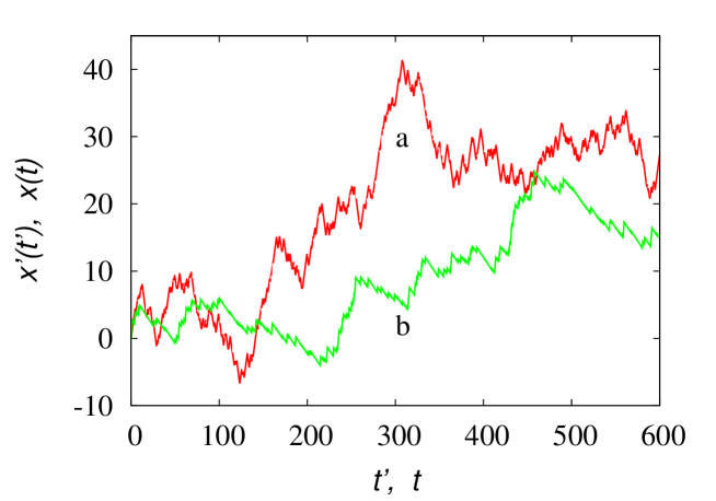
To begin with, consider the one-dimensional spatial (1d, for short) Poisson-Kac process eq. (1). Set b0β€²=c=1subscriptsuperscript𝑏′0𝑐1b^{\prime}_{0}=c=1, a0β€²=1superscriptsubscriptπ‘Ž0β€²1a_{0}^{\prime}=1, so that the rest diffusivity equals D0=1/2subscript𝐷012D_{0}=1/2. Figure 1 depicts a portion of a realization of this process in the rest frame Ξ£β€²superscriptΞ£β€²\Sigma^{\prime}, and in an inertial frame moving with respect to Ξ£β€²superscriptΞ£β€²\Sigma^{\prime} at constant velocity w𝑀w.

Refer to caption
Figure 1: Graph of the evolution of a realization of a Poisson-Kac process (b0β€²=c=1superscriptsubscript𝑏0′𝑐1b_{0}^{\prime}=c=1, a0β€²=1superscriptsubscriptπ‘Ž0β€²1a_{0}^{\prime}=1) in the rest frame Ξ£β€²superscriptΞ£β€²\Sigma^{\prime} (line a, i.e., xβ€²(tβ€²x^{\prime}(t^{\prime})), and in the inertial system ΣΣ\Sigma moving with constant velocity w/c=0.8𝑀𝑐0.8w/c=0.8 with respect to Ξ£β€²superscriptΞ£β€²\Sigma^{\prime} (line b, i.e., x​(t)π‘₯𝑑x(t)).

Consider an ensemble of Npsubscript𝑁𝑝N_{p} realizations of the Poisson-Kac process. Each realization can be viewed as a stochastic particle, the dynamics of which follows the microscopic dynamics eq. (1). At time tβ€²=t=0superscript𝑑′𝑑0t^{\prime}=t=0 set xβ€²=0superscriptπ‘₯β€²0x^{\prime}=0 for all the elements of the ensemble. Figure 2 depicts the overall probability density function p​(x,t)𝑝π‘₯𝑑p(x,t) vs the spatial coordinate xπ‘₯x of the moving inertial frame obtained numerically from the stochastic simulations over this ensemble for different values of t𝑑t and for two different relative velocity of the frame ΣΣ\Sigma: w/c=0.8𝑀𝑐0.8w/c=0.8 (panel a), w/c=0.95𝑀𝑐0.95w/c=0.95 (panel b). All the simulations refer to a statistics over Np=105subscript𝑁𝑝superscript105N_{p}=10^{5} particles.

Refer to caption

(a) Refer to caption (b)

Figure 2: Overall probability density function p​(x,t)𝑝π‘₯𝑑p(x,t) vs xπ‘₯x of a Poisson-Kac process (b0β€²=c=1superscriptsubscript𝑏0′𝑐1b_{0}^{\prime}=c=1, a0β€²=1superscriptsubscriptπ‘Ž0β€²1a_{0}^{\prime}=1) in the frame ΣΣ\Sigma at several time instants. Panel (a) refers to w/c=0.8𝑀𝑐0.8w/c=0.8, panel (b) to w/c=0.95𝑀𝑐0.95w/c=0.95. Lines (a) to (d) refer to t=30, 50, 70𝑑305070t=30,\,50,\,70 and 100100100, respectively.

As expected, the pdf’s p​(x,t)𝑝π‘₯𝑑p(x,t) are characterized by a mean values that equals βˆ’w​t𝑀𝑑-w\,t, and by a variance Οƒ2​(t)superscript𝜎2𝑑\sigma^{2}(t) that becomes narrower as w𝑀w increases up to the limit value c=1𝑐1c=1 (compare the corresponding curves in the two panels).

The graph of the variances Οƒ2​(t)superscript𝜎2𝑑\sigma^{2}(t) vs t𝑑t for different values of the relative frame velocity w𝑀w is depicted in figure 3. The arrow in this figure indicates increasing value of w𝑀w from w=0𝑀0w=0 (upper curve), up to w=0.8𝑀0.8w=0.8 (lower curve). For w=0𝑀0w=0, D0=1/2subscript𝐷012D_{0}=1/2 as expected from eq. (3), i.e. Οƒ2​(t)=tsuperscript𝜎2𝑑𝑑\sigma^{2}(t)=t, while as w𝑀w increases the diffusion coefficient D𝐷D, corresponding to half of the slope of the asymptotic linear plot of Οƒ2​(t)superscript𝜎2𝑑\sigma^{2}(t) vs t𝑑t, decreases.

Refer to caption
Figure 3: Οƒ2​(t)superscript𝜎2𝑑\sigma^{2}(t) vs t𝑑t for a 1d Poisson-Kac process (b0β€²=c=1superscriptsubscript𝑏0′𝑐1b_{0}^{\prime}=c=1, a0β€²=1superscriptsubscriptπ‘Ž0β€²1a_{0}^{\prime}=1) in the frame ΣΣ\Sigma for different values of the frame velocity w𝑀w. The arrow indicates increasing values of w/c=0, 0.2, 0.4, 0.6,,0.8w/c=0,\,0.2,\,0.4,\,0.6,,0.8.

Observe that the concept of long-term properties referred to the recombination dynamics amongst the partial probability waves p+superscript𝑝p^{+} and pβˆ’superscript𝑝p^{-} refers to time-scales t≫tminmuch-greater-than𝑑subscript𝑑mint\gg t_{\rm min}, where tmin=1/aβˆ’subscript𝑑min1superscriptπ‘Žt_{\rm min}=1/a^{-}. For instance at v=0.8𝑣0.8v=0.8, tmin=3subscript𝑑min3t_{\rm min}=3, corresponding to a very fast relaxation towards the asymptotic properties compared to the time-scales reported in the abscissa of figure 3.

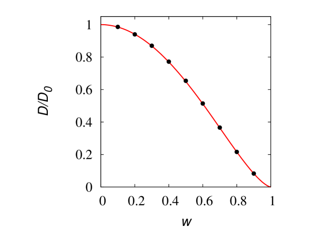
The behavior of the diffusion coefficient D𝐷D vs the relative frame velocity w𝑀w is depicted in figure 4 and it is in perfect agreement with eq. (37).
Refer to caption
Figure 4: D/D0𝐷subscript𝐷0D/D_{0} vs w𝑀w (c=1𝑐1c=1) for a 1d Poisson-Kac process (b0β€²=c=1superscriptsubscript𝑏0′𝑐1b_{0}^{\prime}=c=1, a0β€²=1superscriptsubscriptπ‘Ž0β€²1a_{0}^{\prime}=1). Symbols (βˆ™βˆ™\bullet) represent the results of stochastic simulations, solid line the curve D/D0=Ξ³βˆ’3​(w)=(1βˆ’w2)3/2𝐷subscript𝐷0superscript𝛾3𝑀superscript1superscript𝑀232D/D_{0}=\gamma^{-3}(w)=(1-w^{2})^{3/2}.

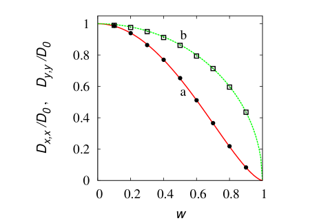
Next, consider higher dimensional stochastic processes. The first example is given by the two-dimensional Kolesnik-Kac model eqs. (38)-(39). We have chosen N=5𝑁5N=5, b0β€²=c=1superscriptsubscript𝑏0′𝑐1b_{0}^{\prime}=c=1, a0β€²=1superscriptsubscriptπ‘Ž0β€²1a_{0}^{\prime}=1, by considering an ensemble of Np=105subscript𝑁𝑝superscript105N_{p}=10^{5} stochastic particles. Figure 5 panel (a) shows the behavior of the diagonal entries Dx,xsubscript𝐷π‘₯π‘₯D_{x,x}, Dy,ysubscript𝐷𝑦𝑦D_{y,y}, obtained from stochastic simulations confirming the theoretical expressions eqs. (75) and (81). The off-diagonal entry is not depicted for the sake of brevity, but is vanishing for any value of the frame velocity w𝑀w.

Refer to caption

(a) Refer to caption (b)

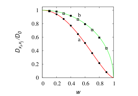
Figure 5: Panel (a): Dx,x/D0subscript𝐷π‘₯π‘₯subscript𝐷0D_{x,x}/D_{0} (symbols βˆ™βˆ™\bullet) and line (a)), and Dy,y/D0subscript𝐷𝑦𝑦subscript𝐷0D_{y,y}/D_{0} (symbols β–‘β–‘\square) and line (b)) vs the relative frame velocity w𝑀w for a two-dimensional Kolesnik-Kac process (N=5𝑁5N=5, b0β€²=c=1superscriptsubscript𝑏0′𝑐1b_{0}^{\prime}=c=1, a0β€²=1superscriptsubscriptπ‘Ž0β€²1a_{0}^{\prime}=1). Line (a) represents the function Ξ³βˆ’3​(w)superscript𝛾3𝑀\gamma^{-3}(w), eq. (75), line (b) the function Ξ³βˆ’1​(w)superscript𝛾1𝑀\gamma^{-1}(w), eq. (81). Symbols (βˆ™βˆ™\bullet) and (β–‘β–‘\square) depict the results of stochastic simulations for Dx,xsubscript𝐷π‘₯π‘₯D_{x,x} and Dy,ysubscript𝐷𝑦𝑦D_{y,y}, respectively. Panel (b): Diagonal diffusivities for the three-dimensional Poisson-Kac process eq. (93) with b0β€²=c=1subscript𝑏superscript0′𝑐1b_{0^{\prime}}=c=1, a0=1subscriptπ‘Ž01a_{0}=1. Symbols represent the results of stochastic simulations: (βˆ™βˆ™\bullet) refer to Dx1,x1subscript𝐷subscriptπ‘₯1subscriptπ‘₯1D_{x_{1},x_{1}}, (β–‘β–‘\square) and (β– β– \blacksquare) to Dx2,x2subscript𝐷subscriptπ‘₯2subscriptπ‘₯2D_{x_{2},x_{2}} and Dx3,x3subscript𝐷subscriptπ‘₯3subscriptπ‘₯3D_{x_{3},x_{3}}, respectively. Lines (a) and (b) are the same as in panel (a).

Finally, let us consider a three-dimensional model, namely the Poisson-Kac process

d​xi′​(tβ€²)=b0′​(βˆ’1)Ο‡i​(tβ€²)​d​tβ€²,i=1,2,3formulae-sequence𝑑superscriptsubscriptπ‘₯𝑖′superscript𝑑′superscriptsubscript𝑏0β€²superscript1subscriptπœ’π‘–superscript𝑑′𝑑superscript𝑑′𝑖123dx_{i}^{\prime}(t^{\prime})=b_{0}^{\prime}\,(-1)^{\chi_{i}(t^{\prime})}\,dt^{\prime}\;,\qquad i=1,2,3 (93)

where Ο‡i​(tβ€²)subscriptπœ’π‘–superscript𝑑′\chi_{i}(t^{\prime}), i=1,2,3𝑖123i=1,2,3 are three Poisson processes, statistically independent of each other, characterized by the same values of the reference velocity b0β€²superscriptsubscript𝑏0β€²b_{0}^{\prime} and of the transition rate a0β€²superscriptsubscriptπ‘Ž0β€²a_{0}^{\prime}. This model, statistically described by means of eight partial probability density functions, converges - for b0β€²,a0β€²β†’βˆžβ†’superscriptsubscript𝑏0β€²superscriptsubscriptπ‘Ž0β€²b_{0}^{\prime},a_{0}^{\prime}\rightarrow\infty, keeping fixed the ratio (b0β€²)2/a0β€²superscriptsuperscriptsubscript𝑏0β€²2superscriptsubscriptπ‘Ž0β€²(b_{0}^{\prime})^{2}/a_{0}^{\prime} - to an isotropic three-dimensional parabolic diffusion equation for the overall pdf p​(𝐱′,tβ€²)𝑝superscript𝐱′superscript𝑑′p({\bf x}^{\prime},t^{\prime}) with diffusion coefficient equal to D0subscript𝐷0D_{0} given by eq. (3).

Let ΣΣ\Sigma be an inertial frame moving with a constant velocity along the direction x1β€²superscriptsubscriptπ‘₯1β€²x_{1}^{\prime} with respect to Ξ£β€²superscriptΞ£β€²\Sigma^{\prime}. It is expected that eqs. (75) and (81) apply also in this case, providing for the diffusivity tensor Dxi,xjsubscript𝐷subscriptπ‘₯𝑖subscriptπ‘₯𝑗D_{x_{i},x_{j}} in ΣΣ\Sigma the following expression

(Dxi,xj)=D0​(Ξ³βˆ’3​(v)000Ξ³βˆ’1​(v)000Ξ³βˆ’1​(v))subscript𝐷subscriptπ‘₯𝑖subscriptπ‘₯𝑗subscript𝐷0superscript𝛾3𝑣000superscript𝛾1𝑣000superscript𝛾1𝑣(D_{x_{i},x_{j}})=D_{0}\,\left(\begin{array}[]{ccc}\gamma^{-3}(v)&\qquad 0&\qquad 0\\ \qquad 0&\gamma^{-1}(v)&0\\ 0&0&\gamma^{-1}(v)\end{array}\right) (94)

The results of stochastic simulations over an ensamble of Np=105subscript𝑁𝑝superscript105N_{p}=10^{5} particles are depicted in panel (b) of figure 5 confirming the theoretical prediction. Off-diagonal entries (not shown) prove to be vanishing.

8 Stochastic action invariance

There is a striking analogy between the results expressed by eq. (94) and the scaling of the longitudinal and transveral masses. Albeit the concepts of longitudinal and transversal masses, introduced by Einstein [30] in the early days of relativity theory (see also [31]), are nowadays considered obsolete, their use in the present context is convenient in order to derive an interesting by-product of eq. (94).

Consider the equation of motion of a particle of rest mass m0=E0/c2subscriptπ‘š0subscript𝐸0superscript𝑐2m_{0}=E_{0}/c^{2} in an intertial frame ΣΣ\Sigma moving with velocity w𝑀w along the x1subscriptπ‘₯1x_{1}-axis. Introduce the diagonal mass tensor 𝐦=diag​(mβŸ‚,mβˆ₯,mβˆ₯)𝐦diagsubscriptπ‘šperpendicular-tosubscriptπ‘šparallel-tosubscriptπ‘šparallel-to{\bf m}=\mbox{diag}(m_{\perp},m_{\parallel},m_{\parallel}), where mβŸ‚subscriptπ‘šperpendicular-tom_{\perp} and mβˆ₯subscriptπ‘šparallel-tom_{\parallel} are the longitudinal and transversal masses, respectively (the mass tensor enters the three-dimensional expression of the relativistic Newton equation). The relativistic scaling of 𝐦𝐦{\bf m} is expressed by

𝐦=m0​(Ξ³3​(w)000γ​(w)000γ​(w))𝐦subscriptπ‘š0superscript𝛾3𝑀000𝛾𝑀000𝛾𝑀{\bf m}=m_{0}\,\left(\begin{array}[]{ccc}\gamma^{3}(w)&0&0\\ 0&\gamma(w)&0\\ 0&0&\gamma(w)\end{array}\right) (95)

From eq. (94) it follows that the product 𝐦​𝐃𝐦𝐃{\bf m}\,{\bf D} of a particle performing purely diffusive stochastic motion is an isotropic tensor

𝐦​𝐃=m0​D0β€‹πˆπ¦πƒsubscriptπ‘š0subscript𝐷0𝐈{\bf m}\,{\bf D}=m_{0}\,D_{0}\,{\bf I} (96)

and the non-vanishing diagonal entries are relativistically invariant, i.e., they do not depend on the velocity w𝑀w.

This observation, can be expressed as follows: if a particle possessing rest mass m0subscriptπ‘š0m_{0} evolves according to a relativistically stochastic process admitting in a given inertial frame Ξ£β€²superscriptΞ£β€²\Sigma^{\prime} no convective contribution and an isotropic diffusivity tensor 𝐃′=D0β€‹πˆsuperscript𝐃′subscript𝐷0𝐈{\bf D}^{\prime}=D_{0}\,{\bf I} (this specific inertial frame can be referred to as the rest frame for the stochastic motion), then in all the inertial frames ΣΣ\Sigma moving with respect to Ξ£β€²superscriptΞ£β€²\Sigma^{\prime} at constant velocity w𝑀w, say along the x1subscriptπ‘₯1x_{1}-coordinate, the product 𝐦​𝐃𝐦𝐃{\bf m}\,{\bf D} of the mass tensor times the diffusivity tensor is invariant with respect to w𝑀w and equal to m0​D0β€‹πˆsubscriptπ‘š0subscript𝐷0𝐈m_{0}\,D_{0}\,{\bf I}.

The quantity hm=m0​D0subscriptβ„Žπ‘šsubscriptπ‘š0subscript𝐷0h_{m}=m_{0}\,D_{0} has the physical dimension of kg​m2​/skgsuperscriptm2/s\mbox{kg}\,\mbox{m}^{2}\mbox{/s}, i.e., it corresponds to an action, so that eq. (97) implies that the stochastic action hmsubscriptβ„Žπ‘šh_{m} is relativistically invariant. It does not depend on the relative frame velocity, but eventually it can depend on the particle rest mass.

We can develop further this concept by introducing quantum mechanical considerations. From the well known correspondence between the Schrâdinger equation and stochastic processes [32, 33], usually obtained via an analytic continuation of the time coordinate towards the imaginary axis, the quantum mechanical representation of the kinetic energy of a free particle corresponds to an effective quantum diffusivity Dquantumsubscript𝐷quantumD_{\rm quantum} expressed by

Dquantum=ℏ2​m0subscript𝐷quantumPlanck-constant-over-2-pi2subscriptπ‘š0D_{\rm quantum}=\frac{\hbar}{2\,m_{0}} (97)

Therefore, for a free quantum particle, D0=Dquantumsubscript𝐷0subscript𝐷quantumD_{0}=D_{\rm quantum}, and eqs. (96)-(97) provide

hm=ℏ2subscriptβ„Žπ‘šPlanck-constant-over-2-pi2h_{m}=\frac{\hbar}{2} (98)

i.e., the stochastic action is not only relativistically invariant but also independent of the particle rest mass. It indicates that in a stochastic representation of quantum motion, the basic constraint induced by quantization and by the Lorentz transformation is the relativistic invariance of the product of the mass tensor times the effective diffusivity tensor that, in any inertial frame, returns an isotropic tensor with eigenvalues equal to ℏ/2Planck-constant-over-2-pi2\hbar/2,

𝐦​𝐃=ℏ2β€‹πˆπ¦πƒPlanck-constant-over-2-pi2𝐈{\bf m}\,{\bf D}=\frac{\hbar}{2}\,{\bf I} (99)

Equation (99) can be viewed as a stochastic quantization rule emerging from special relativity. Its implication will be explored elsewhere. However, a qualitative indication emerging from eq. (99) is that, even in the low-energy limit, i.e., for the SchrΓΆdinger equation (not speaking of the Dirac counterpart), a stochastic interpretation of its formal structure could be properly grounded on a relativistic covariant framework. This implies that the source of stochasticity originating quantum uncertainty, should also possess covariant properties. The natural candidate possessing all these requirements is the zero-point energy fluctuations of the electromagnetic field [34]. A thorough analysis of this issue will be addressed in forthcoming works.

9 Analysis of the diffusivity tensor: Space-Time Diffusion

The results obtained for Poisson-Kac processes are confirmed and generalized by the study of discrete stochastic space-time dynamics which is addressed in this Section. This extension provides a general expression for the relativitic transformation of the diffusivity tensor.

9.1 Space-Time Diffusion

Discrete Space-Time Diffusion (henceforth STD) processes in ℝNsuperscriptℝ𝑁{\mathbb{R}}^{N} has been originally introduced in [24] in order to describe in a compact way particle transport in periodic arrays of obstacles or localized repulsive potentials. A STD process is defined by the quintuple (N,S,𝝅,{𝐀α}Ξ±=1S,𝝉)𝑁𝑆𝝅superscriptsubscriptsubscript𝐀𝛼𝛼1𝑆𝝉(N,S,\boldsymbol{\pi},\{{\bf A}_{\alpha}\}_{\alpha=1}^{S},\boldsymbol{\tau}), where N𝑁N is the space-dimension, S𝑆S the number of states the random space-time displacements can attain, 𝝅=(Ο€1,…,Ο€S)𝝅subscriptπœ‹1…subscriptπœ‹π‘†\boldsymbol{\pi}=(\pi_{1},\dots,\pi_{S}) a S𝑆S-dimensional probability vector, πα>0subscriptπœ‹π›Ό0\pi_{\alpha}>0, Ξ±=1,…,S𝛼1…𝑆\alpha=1,\dots,S, βˆ‘Ξ±=1Sπα=1superscriptsubscript𝛼1𝑆subscriptπœ‹π›Ό1\sum_{\alpha=1}^{S}\pi_{\alpha}=1, 𝐀αsubscript𝐀𝛼{\bf A}_{\alpha}, Ξ±=1,…,S𝛼1…𝑆\alpha=1,\dots,S, are given (constant) space-displacements in ℝNsuperscriptℝ𝑁{\mathbb{R}}^{N}, and 𝝉=(Ο„1,…,Ο„S)𝝉subscript𝜏1…subscriptπœπ‘†\boldsymbol{\tau}=(\tau_{1},\dots,\tau_{S}) the corresponding time intervals τα>0subscriptπœπ›Ό0\tau_{\alpha}>0.

Consider an inertial system ΣΣ\Sigma defined by the space-time coordinates (𝐱,t)𝐱𝑑({\bf x},t). The dynamics of a STD process in ΣΣ\Sigma is defined with respect to a discrete β€œiteration time” n=0,1,…𝑛01…n=0,1,\dots as

(𝐱n+1,tn)=(𝐱n+𝐀α,tn+τα)Prob. ​παsubscript𝐱𝑛1subscript𝑑𝑛subscript𝐱𝑛subscript𝐀𝛼subscript𝑑𝑛subscriptπœπ›ΌProb.Β subscriptπœ‹π›Ό({\bf x}_{n+1},t_{n})=({\bf x}_{n}+{\bf A}_{\alpha},t_{n}+\tau_{\alpha})\qquad\mbox{Prob. }\pi_{\alpha} (100)

Ξ±=1,…,S𝛼1…𝑆\alpha=1,\dots,S. Suppose that the process is defined at n=0𝑛0n=0 such that 𝐱0=0subscript𝐱00{\bf x}_{0}=0, t0=0subscript𝑑00t_{0}=0, so that no issues of simultaneity arise. Eq. (100) can be viewed as a stroboscopic sampling of a stochastic process in the reference system ΣΣ\Sigma.

From the theory of STD processes developed in [24], the long-term evolution for the probability density p​(𝐱,t)𝑝𝐱𝑑p({\bf x},t), 𝐱=(x1,…,xN)𝐱subscriptπ‘₯1…subscriptπ‘₯𝑁{\bf x}=(x_{1},\dots,x_{N}), associated with eq. (100) converges to the solution of an effective constant-coefficient advection-diffusion equation

βˆ‚tp​(𝐱,t)=βˆ’βˆ‘k=1Nvkβ€‹βˆ‚xkp​(𝐱,t)+βˆ‘h,k=1NDh,kβ€‹βˆ‚xhβˆ‚xkp​(𝐱,t)subscript𝑑𝑝𝐱𝑑superscriptsubscriptπ‘˜1𝑁subscriptπ‘£π‘˜subscriptsubscriptπ‘₯π‘˜π‘π±π‘‘superscriptsubscriptβ„Žπ‘˜1𝑁subscriptπ·β„Žπ‘˜subscriptsubscriptπ‘₯β„Žsubscriptsubscriptπ‘₯π‘˜π‘π±π‘‘\partial_{t}p({\bf x},t)=-\sum_{k=1}^{N}v_{k}\,\partial_{x_{k}}p({\bf x},t)+\sum_{h,k=1}^{N}D_{h,k}\,\partial_{x_{h}}\partial_{x_{k}}p({\bf x},t) (101)

where βˆ‚t=βˆ‚/βˆ‚tsubscript𝑑𝑑\partial_{t}=\partial/\partial t, βˆ‚xk=βˆ‚/βˆ‚xksubscriptsubscriptπ‘₯π‘˜subscriptπ‘₯π‘˜\partial_{x_{k}}=\partial/\partial x_{k}, and 𝐯=(v1,…,vN)𝐯subscript𝑣1…subscript𝑣𝑁{\bf v}=(v_{1},\dots,v_{N}), 𝐃=(Dh,k)h,k=1N𝐃superscriptsubscriptsubscriptπ·β„Žπ‘˜β„Žπ‘˜1𝑁{\bf D}=(D_{h,k})_{h,k=1}^{N} represent the constant effective velocity vector and tensor diffusivity, respectively.

Introducing the quantities

Vt(n)superscriptsubscript𝑉𝑑𝑛\displaystyle V_{t}^{(n)} =\displaystyle= βˆ‘Ξ±=1Sπα​τα,Vk(n)=βˆ‘Ξ±=1Sπα​AΞ±,k,k=1,…,Nformulae-sequencesuperscriptsubscript𝛼1𝑆subscriptπœ‹π›Όsubscriptπœπ›Όsuperscriptsubscriptπ‘‰π‘˜π‘›superscriptsubscript𝛼1𝑆subscriptπœ‹π›Όsubscriptπ΄π›Όπ‘˜π‘˜1…𝑁\displaystyle\sum_{\alpha=1}^{S}\pi_{\alpha}\,\tau_{\alpha}\,,\qquad V_{k}^{(n)}=\sum_{\alpha=1}^{S}\pi_{\alpha}\,A_{\alpha,k}\,,\;\;k=1,\dots,N
Dt(n)superscriptsubscript𝐷𝑑𝑛\displaystyle D_{t}^{(n)} =\displaystyle= 12​[βˆ‘Ξ±=1Sπα​τα2βˆ’(Vt(n))2],12delimited-[]superscriptsubscript𝛼1𝑆subscriptπœ‹π›Όsuperscriptsubscriptπœπ›Ό2superscriptsuperscriptsubscript𝑉𝑑𝑛2\displaystyle\frac{1}{2}\left[\sum_{\alpha=1}^{S}\pi_{\alpha}\,\tau_{\alpha}^{2}-\left(V_{t}^{(n)}\right)^{2}\right]\,,\qquad
Dt,k(n)superscriptsubscriptπ·π‘‘π‘˜π‘›\displaystyle D_{t,k}^{(n)} =\displaystyle= 12​[βˆ‘Ξ±=1Sπα​τα​AΞ±,kβˆ’Vt(n)​Vk(n)],k=1,…,Nformulae-sequence12delimited-[]superscriptsubscript𝛼1𝑆subscriptπœ‹π›Όsubscriptπœπ›Όsubscriptπ΄π›Όπ‘˜superscriptsubscript𝑉𝑑𝑛superscriptsubscriptπ‘‰π‘˜π‘›π‘˜1…𝑁\displaystyle\frac{1}{2}\left[\sum_{\alpha=1}^{S}\pi_{\alpha}\,\tau_{\alpha}\,A_{\alpha,k}-V_{t}^{(n)}\,V_{k}^{(n)}\right]\,,\;\;k=1,\dots,N
Dh,k(n)superscriptsubscriptπ·β„Žπ‘˜π‘›\displaystyle D_{h,k}^{(n)} =\displaystyle= 12​[βˆ‘Ξ±=1Sπα​AΞ±,h​AΞ±,kβˆ’Vh(n)​Vk(n)],h,k=1,…,Nformulae-sequence12delimited-[]superscriptsubscript𝛼1𝑆subscriptπœ‹π›Όsubscriptπ΄π›Όβ„Žsubscriptπ΄π›Όπ‘˜superscriptsubscriptπ‘‰β„Žπ‘›superscriptsubscriptπ‘‰π‘˜π‘›β„Žπ‘˜1…𝑁\displaystyle\frac{1}{2}\left[\sum_{\alpha=1}^{S}\pi_{\alpha}\,A_{\alpha,h}\,A_{\alpha,k}-V_{h}^{(n)}\,V_{k}^{(n)}\right]\,,\;\;h,k=1,\dots,N (102)

where AΞ±,ksubscriptπ΄π›Όπ‘˜A_{\alpha,k} is the kπ‘˜k-th entry of the space-displacement vector 𝐀αsubscript𝐀𝛼{\bf A}_{\alpha}, the effective transport parameters attain the expression

vk=Vk(n)Vt(n),k=1,…,Nformulae-sequencesubscriptπ‘£π‘˜superscriptsubscriptπ‘‰π‘˜π‘›superscriptsubscriptπ‘‰π‘‘π‘›π‘˜1…𝑁v_{k}=\frac{V_{k}^{(n)}}{V_{t}^{(n)}}\,,\;\;\;k=1,\dots,N (103)

and

Dh,k=Dt(n)​Vh(n)​Vk(n)(Vt(n))3βˆ’[Dt,h(n)​Vk(n)+Dt,k(n)​Vh(n)](Vt(n))2+Dh,k(n)Vt(n)subscriptπ·β„Žπ‘˜superscriptsubscript𝐷𝑑𝑛superscriptsubscriptπ‘‰β„Žπ‘›superscriptsubscriptπ‘‰π‘˜π‘›superscriptsuperscriptsubscript𝑉𝑑𝑛3delimited-[]superscriptsubscriptπ·π‘‘β„Žπ‘›superscriptsubscriptπ‘‰π‘˜π‘›superscriptsubscriptπ·π‘‘π‘˜π‘›superscriptsubscriptπ‘‰β„Žπ‘›superscriptsuperscriptsubscript𝑉𝑑𝑛2superscriptsubscriptπ·β„Žπ‘˜π‘›superscriptsubscript𝑉𝑑𝑛D_{h,k}=\frac{D_{t}^{(n)}\,V_{h}^{(n)}\,V_{k}^{(n)}}{\left(V_{t}^{(n)}\right)^{3}}-\frac{\left[D_{t,h}^{(n)}\,V_{k}^{(n)}+D_{t,k}^{(n)}\,V_{h}^{(n)}\right]}{\left(V_{t}^{(n)}\right)^{2}}+\frac{D_{h,k}^{(n)}}{V_{t}^{(n)}} (104)

h=k=1,…,Nformulae-sequenceβ„Žπ‘˜1…𝑁h=k=1,\dots,N. Observe that the quantities expressed by eqs. (102) represent the effective space-time velocity and diffusivities parametrized with respect to the discrete iteration time n𝑛n.

9.2 Relativistic analysis

Let eq. (100) be the dynamic description of a stochastic process in ΣΣ\Sigma, and let Ξ£β€²superscriptΞ£β€²\Sigma^{\prime} another inertial frame, the space-time coordinate of which are (𝐱′,tβ€²)superscript𝐱′superscript𝑑′({\bf x}^{\prime},t^{\prime}), moving with respect to ΣΣ\Sigma with constant relative velocity w𝑀w along the x1subscriptπ‘₯1x_{1}-axis. Set c=1𝑐1c=1 for the light speed in vacuo, so that w∈(βˆ’1,1)𝑀11w\in(-1,1).

By the requirements of special relativity, the velocities of the STD process (100) should be bounded by c𝑐c, which implies that

|𝐀|Ξ±<ταα=1,…,Sformulae-sequencesubscript𝐀𝛼subscriptπœπ›Όπ›Ό1…𝑆|{\bf A}|_{\alpha}<\tau_{\alpha}\qquad\alpha=1,\dots,S (105)

For simplicity, consider the case N=2𝑁2N=2, i.e., a spatial two-dimensional model. In Ξ£β€²superscriptΞ£β€²\Sigma^{\prime} the STD process (100) is described by the evolution equation

(𝐱n+1β€²,tnβ€²)=(𝐱nβ€²+𝐀α′,tn+τα′)Prob. ​παsuperscriptsubscript𝐱𝑛1β€²superscriptsubscript𝑑𝑛′superscriptsubscript𝐱𝑛′superscriptsubscript𝐀𝛼′subscript𝑑𝑛superscriptsubscriptπœπ›Όβ€²Prob.Β subscriptπœ‹π›Ό({\bf x}_{n+1}^{\prime},t_{n}^{\prime})=({\bf x}_{n}^{\prime}+{\bf A}_{\alpha}^{\prime},t_{n}+\tau_{\alpha}^{\prime})\qquad\mbox{Prob. }\pi_{\alpha} (106)

Ξ±=1,…,S𝛼1…𝑆\alpha=1,\dots,S, expressed with respect to the space-time coordinates of Ξ£β€²superscriptΞ£β€²\Sigma^{\prime}, where the displacements 𝐀α′superscriptsubscript𝐀𝛼′{\bf A}_{\alpha}^{\prime}, τα′superscriptsubscriptπœπ›Όβ€²\tau_{\alpha}^{\prime} are related to 𝐀αsubscript𝐀𝛼{\bf A}_{\alpha}, ταsubscriptπœπ›Ό\tau_{\alpha} by a Lorentz boost

τα′superscriptsubscriptπœπ›Όβ€²\displaystyle\tau_{\alpha}^{\prime} =\displaystyle= γ​(w)​(Ο„Ξ±βˆ’w​AΞ±,1)𝛾𝑀subscriptπœπ›Όπ‘€subscript𝐴𝛼1\displaystyle\gamma(w)\,(\tau_{\alpha}-w\,A_{\alpha,1})
AΞ±,1β€²superscriptsubscript𝐴𝛼1β€²\displaystyle A_{\alpha,1}^{\prime} =\displaystyle= γ​(w)​(AΞ±,1βˆ’w​τα)𝛾𝑀subscript𝐴𝛼1𝑀subscriptπœπ›Ό\displaystyle\gamma(w)\,(A_{\alpha,1}-w\,\tau_{\alpha}) (107)
AΞ±,2β€²superscriptsubscript𝐴𝛼2β€²\displaystyle A_{\alpha,2}^{\prime} =\displaystyle= AΞ±,2subscript𝐴𝛼2\displaystyle A_{\alpha,2}

Given 𝐀α′superscriptsubscript𝐀𝛼′{\bf A}_{\alpha}^{\prime} and τα′superscriptsubscriptπœπ›Όβ€²\tau_{\alpha}^{\prime}, Ξ±=1,…,S𝛼1…𝑆\alpha=1,\dots,S, eqs. (102)-(104) can be applied to derive the effective transport parameters measured in Ξ£β€²superscriptΞ£β€²\Sigma^{\prime}.

As regards the effective parameters with respect to the iteration time n𝑛n, elementary algebra provides

Vt′⁣(n)=γ​(w)​(Vt(n)βˆ’w​V1(n)),V1′⁣(n)=γ​(w)​(V1(n)βˆ’w​Vt(n)),V2′⁣(n)=V2(n)formulae-sequencesuperscriptsubscript𝑉𝑑′𝑛𝛾𝑀superscriptsubscript𝑉𝑑𝑛𝑀superscriptsubscript𝑉1𝑛formulae-sequencesuperscriptsubscript𝑉1′𝑛𝛾𝑀superscriptsubscript𝑉1𝑛𝑀superscriptsubscript𝑉𝑑𝑛superscriptsubscript𝑉2′𝑛superscriptsubscript𝑉2𝑛V_{t}^{\prime\,(n)}=\gamma(w)\,(V_{t}^{(n)}-w\,V_{1}^{(n)})\,,\qquad V_{1}^{\prime\,(n)}=\gamma(w)\,(V_{1}^{(n)}-w\,V_{t}^{(n)})\,,\qquad V_{2}^{\prime\,(n)}=V_{2}^{(n)} (108)

and

Dt′⁣(n)superscriptsubscript𝐷𝑑′𝑛\displaystyle D_{t}^{\prime\,(n)} =\displaystyle= Ξ³2​(w)​[Dt(n)βˆ’2​w​Dt,1(n)+w2​D1,1(n)]superscript𝛾2𝑀delimited-[]superscriptsubscript𝐷𝑑𝑛2𝑀superscriptsubscript𝐷𝑑1𝑛superscript𝑀2superscriptsubscript𝐷11𝑛\displaystyle\gamma^{2}(w)\,\left[D_{t}^{(n)}-2\,w\,D_{t,1}^{(n)}+w^{2}\,D_{1,1}^{(n)}\right]
Dt,1′⁣(n)superscriptsubscript𝐷𝑑1′𝑛\displaystyle D_{t,1}^{\prime\,(n)} =\displaystyle= Ξ³2​(w)​[(1+w2)​Dt,1(n)βˆ’w​(Dt(n)+D1,1(n))]superscript𝛾2𝑀delimited-[]1superscript𝑀2superscriptsubscript𝐷𝑑1𝑛𝑀superscriptsubscript𝐷𝑑𝑛superscriptsubscript𝐷11𝑛\displaystyle\gamma^{2}(w)\,\left[(1+w^{2})\,D_{t,1}^{(n)}-w\,\left(D_{t}^{(n)}+D_{1,1}^{(n)}\right)\right]
Dt,2′⁣(n)superscriptsubscript𝐷𝑑2′𝑛\displaystyle D_{t,2}^{\prime\,(n)} =\displaystyle= γ​(w)​[Dt,2(n)βˆ’w​D1,2(n)]𝛾𝑀delimited-[]superscriptsubscript𝐷𝑑2𝑛𝑀superscriptsubscript𝐷12𝑛\displaystyle\gamma(w)\,\left[D_{t,2}^{(n)}-w\,D_{1,2}^{(n)}\right] (109)
D1,1′⁣(n)superscriptsubscript𝐷11′𝑛\displaystyle D_{1,1}^{\prime\,(n)} =\displaystyle= Ξ³2​(w)​[D1,1(n)βˆ’2​w​Dt,1(n)+w2​Dt(n)]superscript𝛾2𝑀delimited-[]superscriptsubscript𝐷11𝑛2𝑀superscriptsubscript𝐷𝑑1𝑛superscript𝑀2superscriptsubscript𝐷𝑑𝑛\displaystyle\gamma^{2}(w)\,\left[D_{1,1}^{(n)}-2\,w\,D_{t,1}^{(n)}+w^{2}\,D_{t}^{(n)}\right]
D1,2′⁣(n)superscriptsubscript𝐷12′𝑛\displaystyle D_{1,2}^{\prime\,(n)} =\displaystyle= γ​(w)​[D1,2(n)βˆ’w​Dt,2(n)]𝛾𝑀delimited-[]superscriptsubscript𝐷12𝑛𝑀superscriptsubscript𝐷𝑑2𝑛\displaystyle\gamma(w)\,\left[D_{1,2}^{(n)}-w\,D_{t,2}^{(n)}\right]
D2,2′⁣(n)superscriptsubscript𝐷22′𝑛\displaystyle D_{2,2}^{\prime\,(n)} =\displaystyle= D2,2(n)superscriptsubscript𝐷22𝑛\displaystyle D_{2,2}^{(n)}

For the effective velocities vkβ€²superscriptsubscriptπ‘£π‘˜β€²v_{k}^{\prime} measured in Ξ£β€²superscriptΞ£β€²\Sigma^{\prime}, from eqs. (103) and (108) one obtains

v1β€²=V1′⁣(n)Vt′⁣(n)=v1βˆ’w1βˆ’w​v1v2β€²=V2′⁣(n)Vt′⁣(n)=v2​1βˆ’w21βˆ’w​v1formulae-sequencesuperscriptsubscript𝑣1β€²superscriptsubscript𝑉1′𝑛superscriptsubscript𝑉𝑑′𝑛subscript𝑣1𝑀1𝑀subscript𝑣1superscriptsubscript𝑣2β€²superscriptsubscript𝑉2′𝑛superscriptsubscript𝑉𝑑′𝑛subscript𝑣21superscript𝑀21𝑀subscript𝑣1v_{1}^{\prime}=\frac{V_{1}^{\prime\,(n)}}{V_{t}^{\prime\,(n)}}=\frac{v_{1}-w}{1-w\,v_{1}}\qquad v_{2}^{\prime}=\frac{V_{2}^{\prime\,(n)}}{V_{t}^{\prime\,(n)}}=\frac{v_{2}\,\sqrt{1-w^{2}}}{1-w\,v_{1}} (110)

that correspond to the velocity transformations of special relativity.

More interesting is the transformation of the effective tensor diffusivity, i.e., how 𝐃′superscript𝐃′{\bf D}^{\prime} measured in Ξ£β€²superscriptΞ£β€²\Sigma^{\prime} is related to 𝐃𝐃{\bf D}. To begin with, consider D1,1β€²superscriptsubscript𝐷11β€²D_{1,1}^{\prime}. Eq. (104), expressed in Ξ£β€²superscriptΞ£β€²\Sigma^{\prime}, can be written in the form of an Euclidean scalar product βŸ¨β‹…,β‹…βŸ©β‹…β‹…\langle\cdot,\cdot\rangle, as

D1,1β€²=1(Vt′⁣(n))3β€‹βŸ¨π•~β€²,𝐃~′​𝐕~β€²βŸ©superscriptsubscript𝐷11β€²1superscriptsuperscriptsubscript𝑉𝑑′𝑛3superscript~𝐕′superscript~𝐃′superscript~𝐕′D_{1,1}^{\prime}=\frac{1}{(V_{t}^{\prime\,(n)})^{3}}\,\langle\widetilde{\bf V}^{\prime},\widetilde{\bf D}^{\prime}\,\widetilde{\bf V}^{\prime}\rangle (111)

where

𝐕~β€²=(V1′⁣(n)Vt′⁣(n)),𝐃~β€²=(Dt′⁣(n)βˆ’Dt,1′⁣(n)βˆ’Dt,1′⁣(n)D1,1′⁣(n))formulae-sequencesuperscript~𝐕′superscriptsubscript𝑉1′𝑛superscriptsubscript𝑉𝑑′𝑛superscript~𝐃′superscriptsubscript𝐷𝑑′𝑛superscriptsubscript𝐷𝑑1′𝑛superscriptsubscript𝐷𝑑1′𝑛superscriptsubscript𝐷11′𝑛\widetilde{\bf V}^{\prime}=\left(\begin{array}[]{c}V_{1}^{\prime\,(n)}\\ V_{t}^{\prime\,(n)}\end{array}\right)\,,\qquad\widetilde{\bf D}^{\prime}=\left(\begin{array}[]{cc}D_{t}^{\prime\,(n)}&-D_{t,1}^{\prime\,(n)}\\ -D_{t,1}^{\prime\,(n)}&D_{1,1}^{\prime\,(n)}\end{array}\right) (112)

𝐕~β€²superscript~𝐕′\widetilde{\bf V}^{\prime} is related to 𝐕~=(V1(n),Vt(n))~𝐕superscriptsubscript𝑉1𝑛superscriptsubscript𝑉𝑑𝑛\widetilde{\bf V}=(V_{1}^{(n)},V_{t}^{(n)}) by a Lorentz boost 𝐕~β€²=β„’^w​V~superscript~𝐕′subscript^ℒ𝑀~𝑉\widetilde{\bf V}^{\prime}=\widehat{\mathcal{L}}_{w}\widetilde{V},

β„’^w=(Ξ³βˆ’Ξ³β€‹wβˆ’Ξ³β€‹wΞ³)subscript^ℒ𝑀𝛾𝛾𝑀𝛾𝑀𝛾\widehat{\mathcal{L}}_{w}=\left(\begin{array}[]{cc}\gamma&-\gamma\,w\\ -\gamma w&\gamma\end{array}\right) (113)

The transformation for the entries of 𝐃~β€²superscript~𝐃′\widetilde{\bf D}^{\prime} stemming from eq. (109) is compactly expressed by

(Dt′⁣(n)βˆ’Dt,1′⁣(n)βˆ’Dt,1′⁣(n)D1,1′⁣(n))=Ξ³2​(w)​(1www2w1+w221+w22ww1+w221+w22ww2ww1)​(Dt(n)βˆ’Dt,1(n)βˆ’Dt,1(n)D1,1(n))superscriptsubscript𝐷𝑑′𝑛superscriptsubscript𝐷𝑑1′𝑛superscriptsubscript𝐷𝑑1′𝑛superscriptsubscript𝐷11′𝑛superscript𝛾2𝑀1𝑀𝑀superscript𝑀2𝑀1superscript𝑀221superscript𝑀22𝑀𝑀1superscript𝑀221superscript𝑀22𝑀superscript𝑀2𝑀𝑀1superscriptsubscript𝐷𝑑𝑛superscriptsubscript𝐷𝑑1𝑛superscriptsubscript𝐷𝑑1𝑛superscriptsubscript𝐷11𝑛\left(\begin{array}[]{c}D_{t}^{\prime\,(n)}\\ -D_{t,1}^{\prime\,(n)}\\ -D_{t,1}^{\prime\,(n)}\\ D_{1,1}^{\prime\,(n)}\end{array}\right)=\gamma^{2}(w)\,\left(\begin{array}[]{cccc}1&w&w&w^{2}\\ w&\frac{1+w^{2}}{2}&\frac{1+w^{2}}{2}&w\\ w&\frac{1+w^{2}}{2}&\frac{1+w^{2}}{2}&w\\ w^{2}&w&w&1\end{array}\right)\,\left(\begin{array}[]{c}D_{t}^{(n)}\\ -D_{t,1}^{(n)}\\ -D_{t,1}^{(n)}\\ D_{1,1}^{(n)}\end{array}\right) (114)

The latter transformation can be expressed in tensorial form as D~h,kβ€²=Ξ›h,km,n​D~m,nsuperscriptsubscript~π·β„Žπ‘˜β€²superscriptsubscriptΞ›β„Žπ‘˜π‘šπ‘›subscript~π·π‘šπ‘›\widetilde{D}_{h,k}^{\prime}=\Lambda_{h,k}^{m,n}\,\widetilde{D}_{m,n}, where the fourth-order tensor Ξ›h,km,nsuperscriptsubscriptΞ›β„Žπ‘˜π‘šπ‘›\Lambda_{h,k}^{m,n} accounts for the transformation (114) and Einstein summation notation has been adopted. Consequently, eq. (111) becomes

D1,1β€²=1Ξ³3​(w)​(1βˆ’w​v1)3​Mh,kp,q​V~h​V~k​D~p,q(Vt(n))3superscriptsubscript𝐷11β€²1superscript𝛾3𝑀superscript1𝑀subscript𝑣13superscriptsubscriptπ‘€β„Žπ‘˜π‘π‘žsuperscript~π‘‰β„Žsuperscript~π‘‰π‘˜subscript~π·π‘π‘žsuperscriptsuperscriptsubscript𝑉𝑑𝑛3D_{1,1}^{\prime}=\frac{1}{\gamma^{3}(w)\,(1-w\,v_{1})^{3}}\,\frac{M_{h,k}^{p,q}\,\widetilde{V}^{h}\,\widetilde{V}^{k}\,\widetilde{D}_{p,q}}{\left(V_{t}^{(n)}\right)^{3}} (115)

where V~hsuperscript~π‘‰β„Ž\widetilde{V}^{h}, D~p,qsubscript~π·π‘π‘ž\widetilde{D}_{p,q} are the entries of 𝐕~~𝐕\widetilde{\bf V} and 𝐃~~𝐃\widetilde{\bf D}, above defined, and Mh,kp,q=β„’^w,hp​Λp,qh,k​ℒ^w,kqsuperscriptsubscriptπ‘€β„Žπ‘˜π‘π‘žsuperscriptsubscript^β„’π‘€β„Žπ‘superscriptsubscriptΞ›π‘π‘žβ„Žπ‘˜superscriptsubscript^β„’π‘€π‘˜π‘žM_{h,k}^{p,q}=\widehat{\mathcal{L}}_{w,h}^{p}\,\Lambda_{p,q}^{h,k}\,\widehat{\mathcal{L}}_{w,k}^{q}, β„’^w,hpsuperscriptsubscript^β„’π‘€β„Žπ‘\widehat{\mathcal{L}}_{w,h}^{p} being the entries of the Lorentz boost (113). Developing the algebra, eq. (115) yields the following expression for D1,1β€²superscriptsubscript𝐷11β€²D_{1,1}^{\prime}

D1,1β€²=1Ξ³3​(w)​(1βˆ’w​v1)3=[Dt(n)​(V1(n))2βˆ’2​Dt,1(n)​V1(n)​Vt(n)+D1,1(n)​(Vt(n))2(Vt(n))3]superscriptsubscript𝐷11β€²1superscript𝛾3𝑀superscript1𝑀subscript𝑣13delimited-[]superscriptsubscript𝐷𝑑𝑛superscriptsuperscriptsubscript𝑉1𝑛22superscriptsubscript𝐷𝑑1𝑛superscriptsubscript𝑉1𝑛superscriptsubscript𝑉𝑑𝑛superscriptsubscript𝐷11𝑛superscriptsuperscriptsubscript𝑉𝑑𝑛2superscriptsuperscriptsubscript𝑉𝑑𝑛3D_{1,1}^{\prime}=\frac{1}{\gamma^{3}(w)\,(1-w\,v_{1})^{3}}=\left[\frac{D_{t}^{(n)}\,(V_{1}^{(n)})^{2}-2\,D_{t,1}^{(n)}\,V_{1}^{(n)}\,V_{t}^{(n)}+D_{1,1}^{(n)}\,(V_{t}^{(n)})^{2}}{\left(V_{t}^{(n)}\right)^{3}}\right] (116)

The term under square bracket in eq. (116) is just D1,1subscript𝐷11D_{1,1} as measured in ΣΣ\Sigma, eq. (104) for h=k=1β„Žπ‘˜1h=k=1. Consequently, the trasformation for D1,1subscript𝐷11D_{1,1} attains the compact expression

D1,1β€²=D1,1Ξ³3​(w)​(1βˆ’w​v1)3superscriptsubscript𝐷11β€²subscript𝐷11superscript𝛾3𝑀superscript1𝑀subscript𝑣13D_{1,1}^{\prime}=\frac{D_{1,1}}{\gamma^{3}(w)\,(1-w\,v_{1})^{3}} (117)

Next, consider D1,2β€²superscriptsubscript𝐷12β€²D_{1,2}^{\prime} that in Ξ£β€²superscriptΞ£β€²\Sigma^{\prime} is given by

D1,2β€²=Dt′⁣(n)​V1′⁣(n)​V2′⁣(n)βˆ’Dt,1′⁣(n)​V2′⁣(n)​Vt′⁣(n)βˆ’Dt,2′⁣(n)​V1′⁣(n)​Vt′⁣(n)+D1,2′⁣(n)​(Vt′⁣(n))2(Vt′⁣(n))3superscriptsubscript𝐷12β€²superscriptsubscript𝐷𝑑′𝑛superscriptsubscript𝑉1′𝑛superscriptsubscript𝑉2′𝑛superscriptsubscript𝐷𝑑1′𝑛superscriptsubscript𝑉2′𝑛superscriptsubscript𝑉𝑑′𝑛superscriptsubscript𝐷𝑑2′𝑛superscriptsubscript𝑉1′𝑛superscriptsubscript𝑉𝑑′𝑛superscriptsubscript𝐷12′𝑛superscriptsuperscriptsubscript𝑉𝑑′𝑛2superscriptsuperscriptsubscript𝑉𝑑′𝑛3D_{1,2}^{\prime}=\frac{D_{t}^{\prime\,(n)}\,V_{1}^{\prime\,(n)}\,V_{2}^{\prime\,(n)}-D_{t,1}^{\prime\,(n)}\,V_{2}^{\prime\,(n)}\,V_{t}^{\prime\,(n)}-D_{t,2}^{\prime\,(n)}\,V_{1}^{\prime\,(n)}\,V_{t}^{\prime\,(n)}+D_{1,2}^{\prime\,(n)}\,(V_{t}^{\prime\,(n)})^{2}}{\left(V_{t}^{\prime\,(n)}\right)^{3}} (118)

Substituting the expressions (108)-(109) for the transport parameters in Ξ£β€²superscriptΞ£β€²\Sigma^{\prime} referred to the iteration time n𝑛n as a function of the corresponding quantities in ΣΣ\Sigma, elementary algebra provides the expression

D1,2β€²=D1,2+w​Q1,2Ξ³2​(w)​(1βˆ’w​v1)3superscriptsubscript𝐷12β€²subscript𝐷12𝑀subscript𝑄12superscript𝛾2𝑀superscript1𝑀subscript𝑣13D_{1,2}^{\prime}=\frac{D_{1,2}+w\,Q_{1,2}}{\gamma^{2}(w)\,(1-w\,v_{1})^{3}} (119)

where

Q1,2=D1,1(n)​V2(n)​Vt(n)βˆ’D1,2(n)​V1(n)​Vt(n)βˆ’Dt1(n)​V1(n)​V2(n)+Dt,2(n)​(V1(n))2(Vt′⁣(n))3subscript𝑄12superscriptsubscript𝐷11𝑛superscriptsubscript𝑉2𝑛superscriptsubscript𝑉𝑑𝑛superscriptsubscript𝐷12𝑛superscriptsubscript𝑉1𝑛superscriptsubscript𝑉𝑑𝑛superscriptsubscript𝐷subscript𝑑1𝑛superscriptsubscript𝑉1𝑛superscriptsubscript𝑉2𝑛superscriptsubscript𝐷𝑑2𝑛superscriptsuperscriptsubscript𝑉1𝑛2superscriptsuperscriptsubscript𝑉𝑑′𝑛3Q_{1,2}=\frac{D_{1,1}^{(n)}\,V_{2}^{(n)}\,V_{t}^{(n)}-D_{1,2}^{(n)}\,V_{1}^{(n)}\,V_{t}^{(n)}-D_{t_{1}}^{(n)}\,V_{1}^{(n)}\,V_{2}^{(n)}+D_{t,2}^{(n)}\,(V_{1}^{(n)})^{2}}{\left(V_{t}^{\prime\,(n)}\right)^{3}} (120)

Eq. (104) can be used to express D1,1(n)superscriptsubscript𝐷11𝑛D_{1,1}^{(n)} and D1,2(n)superscriptsubscript𝐷12𝑛D_{1,2}^{(n)} as a function of D1,1subscript𝐷11D_{1,1} and D1,2subscript𝐷12D_{1,2}. In this way, the expression for Q1,2subscript𝑄12Q_{1,2} greatly simplifies, providing Q1,2=D1,1​v2βˆ’D1,2​v1subscript𝑄12subscript𝐷11subscript𝑣2subscript𝐷12subscript𝑣1Q_{1,2}=D_{1,1}\,v_{2}-D_{1,2}\,v_{1}, and consequently the tranformation relation for D1,2β€²superscriptsubscript𝐷12β€²D_{1,2}^{\prime} becomes

D1,2β€²=D1,2+w​(D1,1​v2βˆ’D1,2​v1)Ξ³2​(w)​(1βˆ’w​v1)3superscriptsubscript𝐷12β€²subscript𝐷12𝑀subscript𝐷11subscript𝑣2subscript𝐷12subscript𝑣1superscript𝛾2𝑀superscript1𝑀subscript𝑣13D_{1,2}^{\prime}=\frac{D_{1,2}+w\,(D_{1,1}\,v_{2}-D_{1,2}\,v_{1})}{\gamma^{2}(w)\,(1-w\,v_{1})^{3}} (121)

Finally, consider D2,2β€²superscriptsubscript𝐷22β€²D_{2,2}^{\prime}. From its definition

D2,2β€²=Dt′⁣(n)​(V2′⁣(n))2βˆ’2​Dt,2′⁣(n)​V2′⁣(n)​Vt′⁣(n)+D2,2′⁣(n)​(Vt′⁣(n))2(Vt′⁣(n))3superscriptsubscript𝐷22β€²superscriptsubscript𝐷𝑑′𝑛superscriptsuperscriptsubscript𝑉2′𝑛22superscriptsubscript𝐷𝑑2′𝑛superscriptsubscript𝑉2′𝑛superscriptsubscript𝑉𝑑′𝑛superscriptsubscript𝐷22′𝑛superscriptsuperscriptsubscript𝑉𝑑′𝑛2superscriptsuperscriptsubscript𝑉𝑑′𝑛3D_{2,2}^{\prime}=\frac{D_{t}^{\prime\,(n)}\,(V_{2}^{\prime\,(n)})^{2}-2\,D_{t,2}^{\prime\,(n)}\,V_{2}^{\prime\,(n)}\,V_{t}^{\prime\,(n)}+D_{2,2}^{\prime\,(n)}\,(V_{t}^{\prime\,(n)})^{2}}{\left(V_{t}^{\prime\,(n)}\right)^{3}} (122)

which can be rearranged in the form

D2,2β€²=D2,2+2​w​P2,2+w2​R2,2γ​(w)​(1βˆ’w​v1)3superscriptsubscript𝐷22β€²subscript𝐷222𝑀subscript𝑃22superscript𝑀2subscript𝑅22𝛾𝑀superscript1𝑀subscript𝑣13D_{2,2}^{\prime}=\frac{D_{2,2}+2\,w\,P_{2,2}+w^{2}\,R_{2,2}}{\gamma(w)\,(1-w\,v_{1})^{3}} (123)

where

P2,2subscript𝑃22\displaystyle P_{2,2} =\displaystyle= D1,2(n)​V2(n)​Vt(n)βˆ’D2,2(n)​V1(n)​Vt(n)βˆ’Dt,1(n)​(V2(n))2+Dt,2(n)​V1(n)​V2(n)(Vt′⁣(n))3superscriptsubscript𝐷12𝑛superscriptsubscript𝑉2𝑛superscriptsubscript𝑉𝑑𝑛superscriptsubscript𝐷22𝑛superscriptsubscript𝑉1𝑛superscriptsubscript𝑉𝑑𝑛superscriptsubscript𝐷𝑑1𝑛superscriptsuperscriptsubscript𝑉2𝑛2superscriptsubscript𝐷𝑑2𝑛superscriptsubscript𝑉1𝑛superscriptsubscript𝑉2𝑛superscriptsuperscriptsubscript𝑉𝑑′𝑛3\displaystyle\frac{D_{1,2}^{(n)}\,V_{2}^{(n)}\,V_{t}^{(n)}-D_{2,2}^{(n)}\,V_{1}^{(n)}\,V_{t}^{(n)}-D_{t,1}^{(n)}\,(V_{2}^{(n)})^{2}+D_{t,2}^{(n)}\,V_{1}^{(n)}\,V_{2}^{(n)}}{\left(V_{t}^{\prime\,(n)}\right)^{3}}
R2,2subscript𝑅22\displaystyle R_{2,2} =\displaystyle= D1,1(n)​(V2(n))2βˆ’2​D1,2(n)​V1(n)​V2(n)+D2,2(n)​(V1(n))2(Vt′⁣(n))3superscriptsubscript𝐷11𝑛superscriptsuperscriptsubscript𝑉2𝑛22superscriptsubscript𝐷12𝑛superscriptsubscript𝑉1𝑛superscriptsubscript𝑉2𝑛superscriptsubscript𝐷22𝑛superscriptsuperscriptsubscript𝑉1𝑛2superscriptsuperscriptsubscript𝑉𝑑′𝑛3\displaystyle\frac{D_{1,1}^{(n)}\,(V_{2}^{(n)})^{2}-2\,D_{1,2}^{(n)}\,V_{1}^{(n)}\,V_{2}^{(n)}+D_{2,2}^{(n)}\,(V_{1}^{(n)})^{2}}{\left(V_{t}^{\prime\,(n)}\right)^{3}} (124)

Using eq. (104) to express Dh,k(n)superscriptsubscriptπ·β„Žπ‘˜π‘›D_{h,k}^{(n)} as a function of the diffusivities Dh,ksubscriptπ·β„Žπ‘˜D_{h,k} expressed with respect to the physical time, the expressions for P2,2subscript𝑃22P_{2,2} and R2,2subscript𝑅22R_{2,2} simplifies to obtain for D2,2β€²superscriptsubscript𝐷22β€²D_{2,2}^{\prime} the transformation

D2,2β€²=D2,2+2​w​(D1,2​v2βˆ’D2,2​v1)+w2​(D1,1​v22βˆ’2​D1,2​v1​v2+D2,2​v12)γ​(w)​(1βˆ’w​v1)3superscriptsubscript𝐷22β€²subscript𝐷222𝑀subscript𝐷12subscript𝑣2subscript𝐷22subscript𝑣1superscript𝑀2subscript𝐷11superscriptsubscript𝑣222subscript𝐷12subscript𝑣1subscript𝑣2subscript𝐷22superscriptsubscript𝑣12𝛾𝑀superscript1𝑀subscript𝑣13D_{2,2}^{\prime}=\frac{D_{2,2}+2\,w(D_{1,2}\,v_{2}-D_{2,2}\,v_{1})+w^{2}(D_{1,1}\,v_{2}^{2}-2\,D_{1,2}\,v_{1}\,v_{2}+D_{2,2}\,v_{1}^{2})}{\gamma(w)\,(1-w\,v_{1})^{3}} (125)

9.3 The three-dimensional case

The extension of the transformations developed in the previous paragraph to three-dimensional spatial coordinates in straightforward. As before, suppose that Ξ£β€²superscriptΞ£β€²\Sigma^{\prime} moves relatively to ΣΣ\Sigma with a constant velocity w𝑀w along the x1subscriptπ‘₯1x_{1}-axis.

As regards D1,1β€²superscriptsubscript𝐷11β€²D_{1,1}^{\prime}, D1,hβ€²=Dh,1β€²superscriptsubscript𝐷1β„Žβ€²superscriptsubscriptπ·β„Ž1β€²D_{1,h}^{\prime}=D_{h,1}^{\prime}, Dh,hβ€²superscriptsubscriptπ·β„Žβ„Žβ€²D_{h,h}^{\prime}, with h=2,3β„Ž23h=2,3 the expressions follow from eqs. (117), (121) and (125), namely

D1,1β€²superscriptsubscript𝐷11β€²\displaystyle D_{1,1}^{\prime} =\displaystyle= D1,1Ξ³3​(w)​(1βˆ’w​v1)3subscript𝐷11superscript𝛾3𝑀superscript1𝑀subscript𝑣13\displaystyle\frac{D_{1,1}}{\gamma^{3}(w)\,(1-w\,v_{1})^{3}}
D1,hβ€²superscriptsubscript𝐷1β„Žβ€²\displaystyle D_{1,h}^{\prime} =\displaystyle= D1,h+w​(D1,1​vhβˆ’D1,h​v1)Ξ³2​(w)​(1βˆ’w​v1)3h=2,3formulae-sequencesubscript𝐷1β„Žπ‘€subscript𝐷11subscriptπ‘£β„Žsubscript𝐷1β„Žsubscript𝑣1superscript𝛾2𝑀superscript1𝑀subscript𝑣13β„Ž23\displaystyle\frac{D_{1,h}+w\,(D_{1,1}\,v_{h}-D_{1,h}\,v_{1})}{\gamma^{2}(w)\,(1-w\,v_{1})^{3}}\qquad h=2,3 (126)
Dh,hβ€²superscriptsubscriptπ·β„Žβ„Žβ€²\displaystyle D_{h,h}^{\prime} =\displaystyle= Dh,h+2​w​(D1,h​vhβˆ’Dh,h​v1)+w2​(D1,1​vh2βˆ’2​D1,h​v1​vh+Dh,h​v12)γ​(w)​(1βˆ’w​v1)3h=2,3formulae-sequencesubscriptπ·β„Žβ„Ž2𝑀subscript𝐷1β„Žsubscriptπ‘£β„Žsubscriptπ·β„Žβ„Žsubscript𝑣1superscript𝑀2subscript𝐷11superscriptsubscriptπ‘£β„Ž22subscript𝐷1β„Žsubscript𝑣1subscriptπ‘£β„Žsubscriptπ·β„Žβ„Žsuperscriptsubscript𝑣12𝛾𝑀superscript1𝑀subscript𝑣13β„Ž23\displaystyle\frac{D_{h,h}+2\,w\,(D_{1,h}\,v_{h}-D_{h,h}\,v_{1})+w^{2}\,(D_{1,1}v_{h}^{2}-2\,D_{1,h}\,v_{1}\,v_{h}+D_{h,h}\,v_{1}^{2})}{\gamma(w)\,(1-w\,v_{1})^{3}}\;\;\;\;h=2,3

The entry D2,3β€²=D3,2β€²superscriptsubscript𝐷23β€²superscriptsubscript𝐷32β€²D_{2,3}^{\prime}=D_{3,2}^{\prime} requires some additional calculations that, following the same approach outlined in the previous paragraph, returns the expression

D2,3β€²=D2,3+w​(D1,2​v3+D1,3​v2βˆ’2​D2,3​v1)+w2​(D1,1​v2​v3βˆ’D1,2​v1​v3βˆ’D1,2​vβˆ’1​v3+D2,3​v12)γ​(w)​(1βˆ’w​v1)3superscriptsubscript𝐷23β€²subscript𝐷23𝑀subscript𝐷12subscript𝑣3subscript𝐷13subscript𝑣22subscript𝐷23subscript𝑣1superscript𝑀2subscript𝐷11subscript𝑣2subscript𝑣3subscript𝐷12subscript𝑣1subscript𝑣3subscript𝐷12𝑣1subscript𝑣3subscript𝐷23superscriptsubscript𝑣12𝛾𝑀superscript1𝑀subscript𝑣13D_{2,3}^{\prime}=\frac{D_{2,3}+w\,(D_{1,2}\,v_{3}+D_{1,3}\,v_{2}-2\,D_{2,3}\,v_{1})+w^{2}\,(D_{1,1}\,v_{2}\,v_{3}-D_{1,2}\,v_{1}\,v_{3}-D_{1,2}\,v-1\,v_{3}+D_{2,3}\,v_{1}^{2})}{\gamma(w)\,(1-w\,v_{1})^{3}} (127)

This completes the analysis of the Lorentzian transformation of the tensor diffusivity referred to two inertial frame in relative motion.

9.4 Numerical simulations

In this paragraph, a numerical validation of the transformation theory for the effective tensor diffusivities is provided. Consider a spatially two-dimensional STD model, N=2𝑁2N=2 and S=3𝑆3S=3, with 𝝅=(0.5,0.1,0.3)𝝅0.50.10.3\boldsymbol{\pi}=(0.5,0.1,0.3), 𝝉=(1,0.6,0.5)𝝉10.60.5\boldsymbol{\tau}=(1,0.6,0.5), and 𝐀1=(0.8,0.4)subscript𝐀10.80.4{\bf A}_{1}=(0.8,0.4), 𝐀2=(βˆ’0.4,0.3)subscript𝐀20.40.3{\bf A}_{2}=(-0.4,0.3) and 𝐀3=(0.48,βˆ’0.05)subscript𝐀30.480.05{\bf A}_{3}=(0.48,-0.05).

Numerical simulations of STD dynamics have been performed by considering an ensemble of 107superscript10710^{7} particles, initially located at the same space-time point (𝐱0subscript𝐱0{\bf x}_{0},t0=0subscript𝑑00t_{0}=0) evolving according to eq. (100). Using the Lorentz boost, the corresponding coordinates 𝐱nβ€²superscriptsubscript𝐱𝑛′{\bf x}_{n}^{\prime}, tnβ€²superscriptsubscript𝑑𝑛′t_{n}^{\prime} in Ξ£β€²superscriptΞ£β€²\Sigma^{\prime} can be derived, and from the linear scaling of the first and second-order (central) moments with respect to tβ€²superscript𝑑′t^{\prime}, the values vkβ€²superscriptsubscriptπ‘£π‘˜β€²v_{k}^{\prime} and Dh,kβ€²superscriptsubscriptπ·β„Žπ‘˜β€²D_{h,k}^{\prime} can be estimated.

Figure 6 depicts the scaling of the second-order central moments Οƒh,k′⁣ 2​(tβ€²)=⟨(xh′​(tβ€²)βˆ’βŸ¨xh​(tβ€²)⟩)​(xk′​(tβ€²)βˆ’βŸ¨xk​(tβ€²)⟩)⟩superscriptsubscriptπœŽβ„Žπ‘˜β€²2superscript𝑑′delimited-⟨⟩superscriptsubscriptπ‘₯β„Žβ€²superscript𝑑′delimited-⟨⟩subscriptπ‘₯β„Žsuperscript𝑑′superscriptsubscriptπ‘₯π‘˜β€²superscript𝑑′delimited-⟨⟩subscriptπ‘₯π‘˜superscript𝑑′\sigma_{h,k}^{\prime\,2}(t^{\prime})=\langle(x_{h}^{\prime}(t^{\prime})-\langle x_{h}(t^{\prime})\rangle)\,(x_{k}^{\prime}(t^{\prime})-\langle x_{k}(t^{\prime})\rangle)\rangle for w=0.7𝑀0.7w=0.7. Solid lines represent the theoretical predictions Οƒh,kβ€²,2​(tβ€²)=2​Dh,k′​tβ€²superscriptsubscriptπœŽβ„Žπ‘˜β€²2superscript𝑑′2superscriptsubscriptπ·β„Žπ‘˜β€²superscript𝑑′\sigma_{h,k}^{\prime,2}(t^{\prime})=2\,D_{h,k}^{\prime}\,t^{\prime}, where Dh,kβ€²superscriptsubscriptπ·β„Žπ‘˜β€²D_{h,k}^{\prime} are given by eqs. (117), (121) and (125), while symbols refer to the results of the numerical simulations of the stochastic STD model.
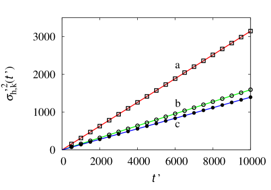
Refer to caption
Figure 6: Behavior of the second order central moments Οƒh,k′⁣ 2​(tβ€²)superscriptsubscriptπœŽβ„Žπ‘˜β€²2superscript𝑑′{\sigma_{h,k}^{\prime\,2}}(t^{\prime}) measured in Ξ£β€²superscriptΞ£β€²\Sigma^{\prime} vs tβ€²superscript𝑑′t^{\prime} for the two-dimensional spatial model described in the main text. Symbols are the results of numerical simulation of the stochastic dynamics, solid lines are the theoretical predictions based on the Einstein scaling Οƒh,k′⁣ 2​(tβ€²)=2​Dh,k′​tβ€²superscriptsubscriptπœŽβ„Žπ‘˜β€²2superscript𝑑′2superscriptsubscriptπ·β„Žπ‘˜β€²superscript𝑑′{\sigma_{h,k}^{\prime\,2}}(t^{\prime})=2\,D_{h,k}^{\prime}\,t^{\prime}, where Dh,kβ€²superscriptsubscriptπ·β„Žπ‘˜β€²D_{h,k}^{\prime} are given by eqs. (117), (121), (125). Line (a) and (β–‘β–‘\square) refer to Οƒ1,1′⁣ 2superscriptsubscript𝜎11β€²2{\sigma_{1,1}^{\prime\,2}}, line (b) and (∘\circ) to Οƒ1,2′⁣ 2superscriptsubscript𝜎12β€²2\sigma_{1,2}^{\prime\,2}, line (c) and (βˆ™βˆ™\bullet) to Οƒ2,2′⁣ 2superscriptsubscript𝜎22β€²2\sigma_{2,2}^{\prime\,2}.

The review of the value of the effective transport parameters measured in Ξ£β€²superscriptΞ£β€²\Sigma^{\prime} vs the relative velocity w𝑀w can be found in figure 7. Panel (a) refers to the effective velocity entries, and panel (b) to the effective tensor diffusivities.
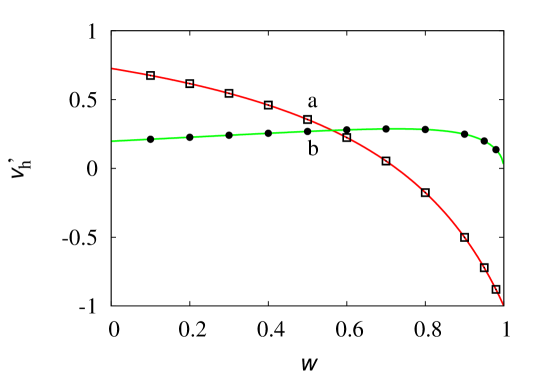
Refer to caption

(a)

Refer to caption

(b)

Figure 7: Effective transport parameters of the spatial two-dimensional STD model described in the main text measured in Ξ£β€²superscriptΞ£β€²\Sigma^{\prime} as a function of the relative frame velocity w𝑀w. Panel (a): effective velocity entries. Line (a) and (β–‘β–‘\square) refer to v1β€²superscriptsubscript𝑣1β€²v_{1}^{\prime}, line (b) and (∘\circ) to v2β€²superscriptsubscript𝑣2β€²v_{2}^{\prime}. Panel (b): effective tensor diffusivities. Line (a) and (β–‘β–‘\square) refer to D1,1β€²superscriptsubscript𝐷11β€²D_{1,1}^{\prime}, line (b) and (∘\circ) to D1,2β€²superscriptsubscript𝐷12β€²D_{1,2}^{\prime}, line (c) and (βˆ™βˆ™\bullet) to D2,2β€²superscriptsubscript𝐷22β€²D_{2,2}^{\prime}.

Apart from the excellent agreement between theory (lines) and simulations (symbols), the behavior of Dh,kβ€²superscriptsubscriptπ·β„Žπ‘˜β€²D_{h,k}^{\prime} vs w𝑀w is highly non-trivial, and the effective diffusivities display a local maximum at some values wh,kβˆ—superscriptsubscriptπ‘€β„Žπ‘˜w_{h,k}^{*} of the relative velocity that depend on hβ„Žh and kπ‘˜k. This phenomenon is a consequence of the presence in the STD model considered of an advective contribution, accounted for by the effective velocity v1subscript𝑣1v_{1}, that is significantly greater than zero. Consequently, the factor (1βˆ’w​v1)3superscript1𝑀subscript𝑣13(1-w\,v_{1})^{3} at the denominator of the expressions for Dh,kβ€²superscriptsubscriptπ·β„Žπ‘˜β€²D_{h,k}^{\prime} modulates their behavior, determining non monotonic effects vs w𝑀w. For example, in the case of D1,1β€²superscriptsubscript𝐷11β€²D_{1,1}^{\prime}, the abscissa w1,1βˆ—superscriptsubscript𝑀11w_{1,1}^{*} of the local maximum equal v1subscript𝑣1v_{1} itself, in the present case v1≃0.726similar-to-or-equalssubscript𝑣10.726v_{1}\simeq 0.726, and D1,1′​(w1,1βˆ—)superscriptsubscript𝐷11β€²superscriptsubscript𝑀11D_{1,1}^{\prime}(w_{1,1}^{*}) is almost three times larger than D1,1subscript𝐷11D_{1,1}.

For wβ†’1→𝑀1w\rightarrow 1, all the diffusivities Dh,kβ€²superscriptsubscriptπ·β„Žπ‘˜β€²D_{h,k}^{\prime} decay to zero, as D1,1β€²βˆΌΞ³βˆ’3​(w)similar-tosuperscriptsubscript𝐷11β€²superscript𝛾3𝑀D_{1,1}^{\prime}\sim\gamma^{-3}(w), D2,2β€²βˆΌΞ³βˆ’1​(w)similar-tosuperscriptsubscript𝐷22β€²superscript𝛾1𝑀D_{2,2}^{\prime}\sim\gamma^{-1}(w), D1,2β€²βˆΌΞ³βˆ’2​(w)similar-tosuperscriptsubscript𝐷12β€²superscript𝛾2𝑀D_{1,2}^{\prime}\sim\gamma^{-2}(w).

The behavior of the tensor diffusivities in Ξ£β€²superscriptΞ£β€²\Sigma^{\prime} for a spatially three-dimensional STD model (N=3𝑁3N=3) is depicted in figure 8. The STD model considered admits S=6𝑆6S=6 states with 𝝅=(0,1,0.2,0.3,0.1,0.2,0.1)𝝅010.20.30.10.20.1\boldsymbol{\pi}=(0,1,0.2,0.3,0.1,0.2,0.1), 𝝉=(1,2,0.5,5,3,0.8)𝝉120.5530.8\boldsymbol{\tau}=(1,2,0.5,5,3,0.8) and 𝐀1=(0.5,βˆ’0.3,0.2)subscript𝐀10.50.30.2{\bf A}_{1}=(0.5,-0.3,0.2), 𝐀2=(1,βˆ’0.4,0.2)subscript𝐀210.40.2{\bf A}_{2}=(1,-0.4,0.2), 𝐀3=(1,0.05,βˆ’0.05)subscript𝐀310.050.05{\bf A}_{3}=(1,0.05,-0.05), 𝐀4=(βˆ’1.5,0.4,0.2)subscript𝐀41.50.40.2{\bf A}_{4}=(-1.5,0.4,0.2), 𝐀5=(1.5,1,0.6)subscript𝐀51.510.6{\bf A}_{5}=(1.5,1,0.6), 𝐀6=(0.3,βˆ’0.2,0.3)subscript𝐀60.30.20.3{\bf A}_{6}=(0.3,-0.2,0.3). Also in this case, the agreement of the theoretical predictions (solid lines) based on eqs. (126)-(127) with respect to the stochastic simulation data (symbols) is excellent.
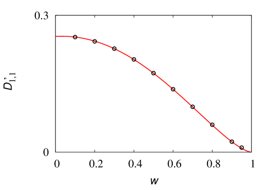
Refer to caption

(a)

Refer to caption

(b)

Figure 8: Effective tensor diffusivities Dh,kβ€²superscriptsubscriptπ·β„Žπ‘˜β€²D_{h,k}^{\prime} vs the relative frame velocity w𝑀w for the spatial three-dimensional model described in the main text. Panel (a): D1,1β€²superscriptsubscript𝐷11β€²D_{1,1}^{\prime} vs w𝑀w. Panel (b): Dh,kβ€²superscriptsubscriptπ·β„Žπ‘˜β€²D_{h,k}^{\prime} vs w𝑀w. Line (a) and (β–‘β–‘\square) refer to D1,2β€²superscriptsubscript𝐷12β€²D_{1,2}^{\prime}, line (b) and (β– β– \blacksquare) to D1,3β€²superscriptsubscript𝐷13β€²D_{1,3}^{\prime}, line (c) and (∘\circ) to D2,2β€²superscriptsubscript𝐷22β€²D_{2,2}^{\prime}, line (d) and (βˆ™βˆ™\bullet) to D2,3β€²superscriptsubscript𝐷23β€²D_{2,3}^{\prime}, line (e) and (β–³β–³\triangle) to D3,3β€²superscriptsubscript𝐷33β€²D_{3,3}^{\prime}.

10 Discussion and implications

In this Section, some implications and observations related to the transformation theory of tensor diffusivities are addressed.

10.1 Observation I - Generality of the transformation

Although we have considered specific stochastic kinematics - Poisson-Kac processes and STD dynamics - eqs. (126)-(127) are of general validity. To support and confirm this claim let us consider a totally different problem, fairly unusual in a relativistic context.

Consider a classical Langevin equation in ℝ3superscriptℝ3{\mathbb{R}}^{3}

d​xh​(t)=vh​d​t+2​Dh​d​wh​(t),h=1,2,3formulae-sequence𝑑subscriptπ‘₯β„Žπ‘‘subscriptπ‘£β„Žπ‘‘π‘‘2subscriptπ·β„Žπ‘‘subscriptπ‘€β„Žπ‘‘β„Ž123dx_{h}(t)=v_{h}\,dt+\sqrt{2\,D_{h}}\,dw_{h}(t)\,,\qquad h=1,2,3 (128)

where wh​(t)subscriptπ‘€β„Žπ‘‘w_{h}(t), h=1,2,3β„Ž123h=1,2,3 are the realizations of three independent Wiener processes, and vhsubscriptπ‘£β„Žv_{h}, Dhsubscriptπ·β„ŽD_{h} are constant. This model is obviously relativistically inconsistent as, by definition, a Wiener process possesses infinite propagation velocity (and so do the xh​(t)subscriptπ‘₯β„Žπ‘‘x_{h}(t) defined by eq. (128)), due to its Gaussian distribution of increments. Therefore, in order to use eq. (128) in the present analysis, this process should be somehow β€œcured”. The β€œcure” we apply is conceptually similar to the classical Wong-Zakai mollification of Brownian motion [35, 36], see also [37].

Let {𝐱~α​(t)}Ξ±=1Npsuperscriptsubscriptsubscript~𝐱𝛼𝑑𝛼1subscript𝑁𝑝\{\widetilde{\bf x}_{\alpha}(t)\}_{\alpha=1}^{N_{p}} be an ensemble of Npsubscript𝑁𝑝N_{p} particles moving according to the stochastic kinematics (128), starting from 𝐱α​(t=0)=0subscript𝐱𝛼𝑑00{\bf x}_{\alpha}(t=0)=0, and let {𝐱~Ξ±(n)=𝐱α​(n​T)}Ξ±=1Npsuperscriptsubscriptsuperscriptsubscript~𝐱𝛼𝑛subscript𝐱𝛼𝑛𝑇𝛼1subscript𝑁𝑝\{\widetilde{\bf x}_{\alpha}^{(n)}={\bf x}_{\alpha}(nT)\}_{\alpha=1}^{N_{p}}, n=0,1,…𝑛01…n=0,1,\dots be their stroboscopic sampling at multiples of the time interval T>0𝑇0T>0. In order to make the sampling {𝐱~Ξ±(n)}Ξ±=1Npsuperscriptsubscriptsuperscriptsubscript~𝐱𝛼𝑛𝛼1subscript𝑁𝑝\{\widetilde{\bf x}_{\alpha}^{(n)}\}_{\alpha=1}^{N_{p}} of the stochastic dynamics relativistically consistent, particle positions should be filtered in order to ensure a propagation velocity less than c𝑐c (c=1𝑐1c=1 in the present analysis). Let {𝐱α(n)}Ξ±=1Npsuperscriptsubscriptsuperscriptsubscript𝐱𝛼𝑛𝛼1subscript𝑁𝑝\{{\bf x}_{\alpha}^{(n)}\}_{\alpha=1}^{N_{p}} be the filtered stroboscopic sampling of {𝐱~Ξ±(n)}Ξ±=1Npsuperscriptsubscriptsuperscriptsubscript~𝐱𝛼𝑛𝛼1subscript𝑁𝑝\{\widetilde{\bf x}_{\alpha}^{(n)}\}_{\alpha=1}^{N_{p}}, obtained in the following way: (i) 𝐱α(0)=𝐱~Ξ±(0)=0superscriptsubscript𝐱𝛼0superscriptsubscript~𝐱𝛼00{\bf x}_{\alpha}^{(0)}=\widetilde{\bf x}_{\alpha}^{(0)}=0, for all Ξ±=1,…,N𝛼1…𝑁\alpha=1,\dots,N; (ii) choose a reference maximum velocity vmax<csubscript𝑣max𝑐v_{\rm max}<c, say vmax=0.99subscript𝑣max0.99v_{\rm max}=0.99; (iii) if δα(n)=‖𝐱~Ξ±(n)βˆ’π±Ξ±(nβˆ’1)β€–>vmax​Tsuperscriptsubscript𝛿𝛼𝑛normsuperscriptsubscript~𝐱𝛼𝑛superscriptsubscript𝐱𝛼𝑛1subscript𝑣max𝑇\delta_{\alpha}^{(n)}=||\widetilde{\bf x}_{\alpha}^{(n)}-{\bf x}_{\alpha}^{(n-1)}||>v_{\rm max}T, i.e., if the relativistic velocity constraint could be locally violated, set for 𝐱α(n)superscriptsubscript𝐱𝛼𝑛{\bf x}_{\alpha}^{(n)} the value

𝐱α(n)=vmax​Tδα(n)​𝐱~Ξ±(n)+(1βˆ’vmax​Tδα(n))​𝐱α(nβˆ’1)superscriptsubscript𝐱𝛼𝑛subscript𝑣max𝑇superscriptsubscript𝛿𝛼𝑛superscriptsubscript~𝐱𝛼𝑛1subscript𝑣max𝑇superscriptsubscript𝛿𝛼𝑛superscriptsubscript𝐱𝛼𝑛1{\bf x}_{\alpha}^{(n)}=\frac{v_{\rm max}\,T}{\delta_{\alpha}^{(n)}}\,\widetilde{\bf x}_{\alpha}^{(n)}+\left(1-\frac{v_{\rm max}\,T}{\delta_{\alpha}^{(n)}}\right)\,{\bf x}_{\alpha}^{(n-1)} (129)

corresponding to a local propagation velocity equal to vmaxsubscript𝑣maxv_{\rm max}. By definition, the filtered stroboscopic sampling {𝐱α(n)}Ξ±=1Npsuperscriptsubscriptsuperscriptsubscript𝐱𝛼𝑛𝛼1subscript𝑁𝑝\{{\bf x}_{\alpha}^{(n)}\}_{\alpha=1}^{N_{p}}, n=0,1,2,…𝑛012…n=0,1,2,\dots is relativistically consistent and can be viewed as a form of Wong-Zakai mollification of the original process, by considering the stochastic trajectories between time instants (nβˆ’1)​T𝑛1𝑇(n-1)T, and n​T𝑛𝑇nT represented by straight lines connecting 𝐱α(nβˆ’1)superscriptsubscript𝐱𝛼𝑛1{\bf x}_{\alpha}^{(n-1)} to 𝐱α(n)superscriptsubscript𝐱𝛼𝑛{\bf x}_{\alpha}^{(n)}.

Consequently, {𝐱α(n)}Ξ±=1Npsuperscriptsubscriptsuperscriptsubscript𝐱𝛼𝑛𝛼1subscript𝑁𝑝\{{\bf x}_{\alpha}^{(n)}\}_{\alpha=1}^{N_{p}} can be viewed as an ensemble of realizations of a relativistically plausible stochastic process defined in an inertial system ΣΣ\Sigma, out of which its transport parameters can be estimated. If the velocities and the diffusivities are small enough, the effective transport parameters estimated in ΣΣ\Sigma practically coincide with vhsubscriptπ‘£β„Žv_{h} and Dhsubscriptπ·β„ŽD_{h}, i.e., with the velocity and diagonal entries of the diffusivity tensor entering eq. (128). Enforcing the Lorentz boost, the effective transport parameters estimated in a reference Ξ£β€²superscriptΞ£β€²\Sigma^{\prime} moving with respect to ΣΣ\Sigma with constant relative velocity w<1𝑀1w<1 along the x1subscriptπ‘₯1x_{1}-axis can be obtained.

Consider for the velocities and diffusivities entering eq. (129) the values v1=asubscript𝑣1π‘Žv_{1}=a, v2=βˆ’0.2subscript𝑣20.2v_{2}=-0.2, v3=0subscript𝑣30v_{3}=0, D1=0.05subscript𝐷10.05D_{1}=0.05, D2=0.03subscript𝐷20.03D_{2}=0.03, D3=0.01subscript𝐷30.01D_{3}=0.01, where aπ‘Ža is a parameter, and let dh,h​(w)=Dh,h′​(w)/Dhsubscriptπ‘‘β„Žβ„Žπ‘€superscriptsubscriptπ·β„Žβ„Žβ€²π‘€subscriptπ·β„Žd_{h,h}(w)=D_{h,h}^{\prime}(w)/D_{h}, for h=1,2,3β„Ž123h=1,2,3, and dh,k​(w)=Dh,h′​(w)subscriptπ‘‘β„Žπ‘˜π‘€superscriptsubscriptπ·β„Žβ„Žβ€²π‘€d_{h,k}(w)=D_{h,h}^{\prime}(w) for hβ‰ kβ„Žπ‘˜h\neq k. Figure 9 panels (a) to (f) depict the six independent entries of dh,k​(w)subscriptπ‘‘β„Žπ‘˜π‘€d_{h,k}(w) as a function of the frame velocity w𝑀w at four different values of the parameter a=0, 0.2, 0.4, 0.6π‘Ž00.20.40.6a=0,\,0.2,\,0.4,\,0.6 controlling convective particle motion along the x1subscriptπ‘₯1x_{1}-direction.

Refer to caption

(a) Refer to caption (b)

Refer to caption

(c) Refer to caption (d)

Refer to caption

(e) Refer to caption (f)

Figure 9: dh,k​(w)subscriptπ‘‘β„Žπ‘˜π‘€d_{h,k}(w) vs w𝑀w for the filtered Wong-Zakai mollification of the process (128) sampled at T=20𝑇20T=20. Lines refer to eqs. (126)-(127), symbols to numerical simulations: lines (a) a=0π‘Ž0a=0, (b) a=0.2π‘Ž0.2a=0.2, (c) a=0.4π‘Ž0.4a=0.4, (d) a=0.6π‘Ž0.6a=0.6. Panel (a) refers to d1,1​(w)subscript𝑑11𝑀d_{1,1}(w), panel (b) to d2,2​(w)subscript𝑑22𝑀d_{2,2}(w), panel (c) to d3,3​(w)subscript𝑑33𝑀d_{3,3}(w), panel (d) to d1,2​(w)=d2,1​(w)subscript𝑑12𝑀subscript𝑑21𝑀d_{1,2}(w)=d_{2,1}(w), panel (e) to d1,3​(w)=d3,1​(w)subscript𝑑13𝑀subscript𝑑31𝑀d_{1,3}(w)=d_{3,1}(w), panel (f) to d2,3​(w)=d3,2​(w)subscript𝑑23𝑀subscript𝑑32𝑀d_{2,3}(w)=d_{3,2}(w).

Simulation results refer to the ensamble {𝐱α(n)}Ξ±=1Npsuperscriptsubscriptsuperscriptsubscript𝐱𝛼𝑛𝛼1subscript𝑁𝑝\{{\bf x}_{\alpha}^{(n)}\}_{\alpha=1}^{N_{p}} obtained from eq. (128) using the Wong-Zakai filtering discussed above with a sampling time T=20𝑇20T=20, and Np=105subscript𝑁𝑝superscript105N_{p}=10^{5}. Stochastic trajectories have been obtained from eq. (128) using a classical Euler-Langevin algorithm with a time step Δ​t=10βˆ’3Δ𝑑superscript103\Delta t=10^{-3}. In the present simulations, involving a rather small ensemble of particles, eq. (129) has never been used, and solely the Wong-Zakai linear interpolation between 𝐱α(nβˆ’1)superscriptsubscript𝐱𝛼𝑛1{\bf x}_{\alpha}^{(n-1)} and 𝐱α(n)superscriptsubscript𝐱𝛼𝑛{\bf x}_{\alpha}^{(n)} has been applied in order to obtain the particle position at constant value of time tβ€²superscript𝑑′t^{\prime} measured in Ξ£β€²superscriptΞ£β€²\Sigma^{\prime}. Solid lines in figure 9 refer to the theoretical predictions based on eqs. (126)-(127), where Dh,k=Dh​dh,ksubscriptπ·β„Žπ‘˜subscriptπ·β„Žsubscriptπ‘‘β„Žπ‘˜D_{h,k}=D_{h}\,d_{h,k}, and Dhsubscriptπ·β„ŽD_{h} are the diagonal diffusivity entering eq. (128). An excellent agreement between theory and stochastic simulations can be observed, confirming the general validity of eqs. (126)-(127).

10.2 Observation 2 - Poisson-Kac processes and the limit for wβ†’c→𝑀𝑐w\rightarrow c

The analysis developed for STD processes is in agreement with the results obtained for the relativistic kinematics of Poisson-Kac processes. In the latter case D1,2=0subscript𝐷120D_{1,2}=0, and the convective contributions are absent, i.e. v1=v2=0subscript𝑣1subscript𝑣20v_{1}=v_{2}=0. Correspondingly, eqs. (126)-(127) predict the scaling of the longitudinal D1,1β€²superscriptsubscript𝐷11β€²D_{1,1}^{\prime} and transversal D2,2β€²superscriptsubscript𝐷22β€²D_{2,2}^{\prime} diffusivities given by eq. (94).

Particularly interesting is the limit of these equations for w𝑀w approaching c=1𝑐1c=1. In this case the measured diffusivities in Ξ£β€²superscriptΞ£β€²\Sigma^{\prime} vanish identically. For an observer that moves close to the velocity of light the contribution of external stochastic perturbations, the intensity of which are related to the diffusivities Dh,kβ€²superscriptsubscriptπ·β„Žπ‘˜β€²D_{h,k}^{\prime}, becomes progressively irrelevant as wβ†’c→𝑀𝑐w\rightarrow c. This issue is discussed in greater detail in [26] which addresses the relativistic relevance of Poisson-Kac processes as the prototype of a covariant stochastic kinematics.

In point of fact, the vanishing properties of Dh,kβ€²superscriptsubscriptπ·β„Žπ‘˜β€²D_{h,k}^{\prime} for wβ†’c→𝑀𝑐w\rightarrow c could have a deeper physical meaning: it indicates that in a reference system moving with a velocity approaching that of light all the external dissipative and irreversible processes associated with stochastic fluctuations decay to zero.

10.3 Observation 3 - Relativity of stochasticity and determinism

There is another interesting implication of the transformation theory of the tensor diffusivity. From eqs. (126)-(127) it follows that the effective diffusivities Dh,kβ€²superscriptsubscriptπ·β„Žπ‘˜β€²D_{h,k}^{\prime} measured in Ξ£β€²superscriptΞ£β€²\Sigma^{\prime} depends on convective velocities vhsubscriptπ‘£β„Žv_{h}. Apart from the term (1βˆ’w​v1)βˆ’3superscript1𝑀subscript𝑣13(1-wv_{1})^{-3}, this dependence enters as factors multiplying the π’ͺ​(w)π’ͺ𝑀{\mathcal{O}}(w), and π’ͺ​(w2)π’ͺsuperscript𝑀2{\mathcal{O}}(w^{2}) terms in the expressions for Dh,kβ€²superscriptsubscriptπ·β„Žπ‘˜β€²D_{h,k}^{\prime}. The only diffusivity entry that is not influenced by these convective contributions is the longitudinal diffusivity since D1,1β€²=D1,1/Ξ³3​(w)​(1βˆ’w​v1)3superscriptsubscript𝐷11β€²subscript𝐷11superscript𝛾3𝑀superscript1𝑀subscript𝑣13D_{1,1}^{\prime}=D_{1,1}/\gamma^{3}(w)(1-wv_{1})^{3}.

This observation suggests that it may happen that a process that is regarded as fully deterministic in a reference system ΣΣ\Sigma appears to possess a stochastic nature in Ξ£β€²superscriptΞ£β€²\Sigma^{\prime} and viceversa. To clarify this concept it is convenient to consider a simple example. Consider a STD process in ΣΣ\Sigma (model I) with N=2𝑁2N=2, S=2𝑆2S=2 characterized by the following parameters

Ο€1=Ο€2=12,Ο„1=Ο„2=1,𝐀1=(0.80.5),𝐀2=(βˆ’0.80.5)formulae-sequencesubscriptπœ‹1subscriptπœ‹212subscript𝜏1subscript𝜏21formulae-sequencesubscript𝐀10.80.5subscript𝐀20.80.5\pi_{1}=\pi_{2}=\frac{1}{2}\,,\qquad\tau_{1}=\tau_{2}=1\,,\qquad{\bf A}_{1}=\left(\begin{array}[]{c}0.8\\ 0.5\end{array}\right)\,,\;\;\;{\bf A}_{2}=\left(\begin{array}[]{c}-0.8\\ 0.5\end{array}\right) (130)

For this process v1=0subscript𝑣10v_{1}=0, v2=0.5subscript𝑣20.5v_{2}=0.5, D1,1=0.32subscript𝐷110.32D_{1,1}=0.32, D1,2=D2,1=D2,2=0subscript𝐷12subscript𝐷21subscript𝐷220D_{1,2}=D_{2,1}=D_{2,2}=0. Let x=x1π‘₯subscriptπ‘₯1x=x_{1}, y=x2𝑦subscriptπ‘₯2y=x_{2}. In the long-term limit, the dynamic of this process in ΣΣ\Sigma is described by the probability density function p​(x,y,t)𝑝π‘₯𝑦𝑑p(x,y,t) that approaches the solution of the parabolic transport equation

βˆ‚tp​(x,y,t)=βˆ’v2β€‹βˆ‚yp​(x,y,t)+D1,1β€‹βˆ‚x2p​(x,y,t)subscript𝑑𝑝π‘₯𝑦𝑑subscript𝑣2subscript𝑦𝑝π‘₯𝑦𝑑subscript𝐷11superscriptsubscriptπ‘₯2𝑝π‘₯𝑦𝑑\partial_{t}p(x,y,t)=-v_{2}\,\partial_{y}p(x,y,t)+D_{1,1}\,\partial_{x}^{2}p(x,y,t) (131)

The marginal probability density py​(y,t)=βˆ«βˆ’βˆžβˆžp​(x,y,t)​𝑑xsubscript𝑝𝑦𝑦𝑑superscriptsubscript𝑝π‘₯𝑦𝑑differential-dπ‘₯p_{y}(y,t)=\int_{-\infty}^{\infty}p(x,y,t)\,dx of the y𝑦y-process satisfies a strictly deterministic advection equation

βˆ‚ypy​(y,t)=βˆ’v2β€‹βˆ‚ypy​(y,t)subscript𝑦subscript𝑝𝑦𝑦𝑑subscript𝑣2subscript𝑦subscript𝑝𝑦𝑦𝑑\partial_{y}p_{y}(y,t)=-v_{2}\,\partial_{y}p_{y}(y,t) (132)

which follows directly form the inspection of the structure of the space-time displacements (130) characterizing this model. Viewed from ΣΣ\Sigma, the evolution of the y𝑦y-dynamics defines a strictly deterministic process.

Consider the same process viewed by Ξ£β€²superscriptΞ£β€²\Sigma^{\prime} moving with respect to ΣΣ\Sigma with constant relative velocity w>0𝑀0w>0 along the xπ‘₯x axis. In this case the entries D1,2β€²superscriptsubscript𝐷12β€²D_{1,2}^{\prime} and D2,2β€²superscriptsubscript𝐷22β€²D_{2,2}^{\prime} of the diffusivity tensor are different from zero, and specifically

D2,2β€²=D1,1​w2​v22γ​(w)​(1βˆ’w​v1)3>0superscriptsubscript𝐷22β€²subscript𝐷11superscript𝑀2superscriptsubscript𝑣22𝛾𝑀superscript1𝑀subscript𝑣130D_{2,2}^{\prime}=\frac{D_{1,1}\,w^{2}v_{2}^{2}}{\gamma(w)\,(1-w\,v_{1})^{3}}>0 (133)

This phenomenon is depicted in figure 10 where the theoretical expressions for D1,2β€²superscriptsubscript𝐷12β€²D_{1,2}^{\prime} and D2,2β€²superscriptsubscript𝐷22β€²D_{2,2}^{\prime} (solid lines) are compared with numerical simulations of the STD (130).
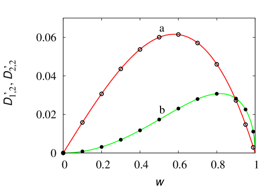
Refer to caption
Figure 10: Diffusivities D1,2β€²superscriptsubscript𝐷12β€²D_{1,2}^{\prime} and D2,2β€²superscriptsubscript𝐷22β€²D_{2,2}^{\prime} measured in Ξ£β€²superscriptΞ£β€²\Sigma^{\prime} vs the relative frame velocity w𝑀w for model I discussed in the main text. Solid lines represent the theoretical predictions (126)-(127), symbols the results of the numerical simulations of the stochastic STD dynamics (130). Line (a) and (∘\circ) refer to D1,2β€²superscriptsubscript𝐷12β€²D_{1,2}^{\prime}, line (b) and (βˆ™βˆ™\bullet) to D2,2β€²superscriptsubscript𝐷22β€²D_{2,2}^{\prime}.

Therefore, the marginal probability density function py′′​(yβ€²,tβ€²)subscriptsuperscript𝑝′superscript𝑦′superscript𝑦′superscript𝑑′p^{\prime}_{y^{\prime}}(y^{\prime},t^{\prime}) for the transversal yβ€²superscript𝑦′y^{\prime}-process in Ξ£β€²superscriptΞ£β€²\Sigma^{\prime} approaches the solution of the advection-diffusion equation

βˆ‚tβ€²py′′​(yβ€²,tβ€²)=βˆ’v2′​pyβ€²+D2,2β€²β€‹βˆ‚yβ€²2py′′​(yβ€²,tβ€²)subscriptsuperscript𝑑′superscriptsubscript𝑝superscript𝑦′′superscript𝑦′superscript𝑑′superscriptsubscript𝑣2β€²subscript𝑝superscript𝑦′superscriptsubscript𝐷22β€²superscriptsubscriptsuperscript𝑦′2superscriptsubscript𝑝superscript𝑦′′superscript𝑦′superscript𝑑′\partial_{t^{\prime}}p_{y^{\prime}}^{\prime}(y^{\prime},t^{\prime})=-v_{2}^{\prime}\,p_{y^{\prime}}+D_{2,2}^{\prime}\,\partial_{y^{\prime}}^{2}p_{y^{\prime}}^{\prime}(y^{\prime},t^{\prime}) (134)

corresponding to the evolution of a stochastic process characterized by an effective diffusivity D2,2β€²>0superscriptsubscript𝐷22β€²0D_{2,2}^{\prime}>0.

Refer to caption
Figure 11: Diffusivities Dh,kβ€²superscriptsubscriptπ·β„Žπ‘˜β€²D_{h,k}^{\prime} vs the relative frame velocity w𝑀w measured in Ξ£β€²superscriptΞ£β€²\Sigma^{\prime} for model II discussed in the main text. Line (a) refers to D1,1β€²superscriptsubscript𝐷11β€²D_{1,1}^{\prime}, line (b) to D1,2β€²superscriptsubscript𝐷12β€²D_{1,2}^{\prime}, line (c) to D2,2β€²superscriptsubscript𝐷22β€²D_{2,2}^{\prime}.

The reverse is also true, by adopting the same argument. Consider a stochastic process in ΣΣ\Sigma for which D2,2β‰ 0subscript𝐷220D_{2,2}\neq 0. By tuning the relative velocity w𝑀w of Ξ£β€²superscriptΞ£β€²\Sigma^{\prime}, it can happen that D2,2β€²=0superscriptsubscript𝐷22β€²0D_{2,2}^{\prime}=0. Consequently, what appears in ΣΣ\Sigma as a stochastic dynamics, is qualified in Ξ£β€²superscriptΞ£β€²\Sigma^{\prime} as strictly deterministic. This phenomenon is depicted in figure 11, where vhsubscriptπ‘£β„Žv_{h} and Dh,ksubscriptπ·β„Žπ‘˜D_{h,k} are given by v1=βˆ’0.5subscript𝑣10.5v_{1}=-0.5, v2=0.433subscript𝑣20.433v_{2}=0.433, D1,1=0.208subscript𝐷110.208D_{1,1}=0.208, D1,2=0.060subscript𝐷120.060D_{1,2}=0.060, D2,2=0.0173subscript𝐷220.0173D_{2,2}=0.0173 (referred to as model II), corresponding to the values of vhβ€²superscriptsubscriptπ‘£β„Žβ€²v_{h}^{\prime} and Dh,kβ€²superscriptsubscriptπ·β„Žπ‘˜β€²D_{h,k}^{\prime} obtained in the STD model depicted in figure 9 at w=0.5𝑀0.5w=0.5, and Ξ£β€²superscriptΞ£β€²\Sigma^{\prime} moves with respect to ΣΣ\Sigma with a negative relative velocity w𝑀w.

10.4 Observation 4 - Diffusivity and Markovian processes in the Minkowski space-time

The concept of tensor diffusivity for a relativistic stochastic process is a long-term emerging property, exactly as for Poisson-Kac processes that are characterized by an effective diffusivity for time-scales much larger than the characteristic recombination time amongst its partial probability waves.

A local (pointwise) diffusivity (possessing the dimension of m2/s) cannot be defined in a Minkowski space-time β„³4subscriptβ„³4{\mathcal{M}}_{4} as it would be necessarily associated with fluctuations possessing a local almost everywhere non-differentiable structure as a function of time, and consequently an unbounded local propagation velocity.

There is another general observation arising from the analysis developed in Section 9. related to the Markovian nature of a stochastic process in a Minkowski space-time.

From the works by Dudley and Hakim quoted in the Introduction, the impossibility of defining a strictly Markovian stochastic kinematics (continuous in time) in β„³4subscriptβ„³4{\mathcal{M}}_{4} follows.

The case of STD processes introduced in Section 9 provides a concrete example of a random dynamics for which the choice of a discrete time parametrization (the iteration time n𝑛n) makes it possible to define a strictly Markovian process in β„³4subscriptβ„³4{\mathcal{M}}_{4}, where space and time variables are stricly treated on equal footing by defining the space-time displacements (𝐀h,Ο„h)subscriptπ€β„Žsubscriptπœβ„Ž({\bf A}_{h},\tau_{h}). The example of STD processes does not contraddict the Dudley-Hakim condition, as the extension with respect to a continuous time variable of STD processes, associated with the concept of hyperbolic homogenization [25], leads to non-strictly Markovian processes in (𝐱,t)𝐱𝑑({\bf x},t) analogous to Poisson-Kac and Generalized Poisson-Kac processes.

10.5 Observation 5 - Skewed structure of the transformation

Given a stochastic process characterized by bounded propagation velocity less than c𝑐c, let 𝐯𝐯{\bf v} and 𝐃𝐃{\bf D} be its effective (long-term) transport properties in a reference frame ΣΣ\Sigma, and 𝐯′superscript𝐯′{\bf v}^{\prime} and 𝐃′superscript𝐃′{\bf D}^{\prime} the corresponding quantities measured in Ξ£β€²superscriptΞ£β€²\Sigma^{\prime}, moving with respect to ΣΣ\Sigma with constant velocity w𝑀w along the x1subscriptπ‘₯1x_{1}-axis. Here 𝐃𝐃{\bf D} and 𝐃′superscript𝐃′{\bf D}^{\prime} are the diffusivity tensors in the two reference frames.

As regards the effective velocity, the transformation from 𝐯𝐯{\bf v} to 𝐯′superscript𝐯′{\bf v}^{\prime} is the classical velocity transformation of special relativity

𝐯′=𝒱w​[𝐯]superscript𝐯′subscript𝒱𝑀delimited-[]𝐯{\bf v}^{\prime}={\mathcal{V}}_{w}[{\bf v}] (135)

for a relative velocity w𝑀w. For the tensor diffusivity the transformation expressed by eqs. (126)-(127) can be compactly indicated as

𝐃′=π’Ÿw​[𝐃,𝐯]superscript𝐃′subscriptπ’Ÿπ‘€πƒπ―{\bf D}^{\prime}={\mathcal{D}}_{w}[{\bf D},{\bf v}] (136)

Observe the skew-product structure of eq. (136) in which the transformation for the diffusivity tensors depends on 𝐯𝐯{\bf v}. In a more compact form, eqs. (135)-(136) can be summarized by the complete transformation of the effective transport parameters (𝐯,𝐃)𝐯𝐃({\bf v},{\bf D}),

(𝐯′,𝐃′)=𝒯w​[(𝐯,𝐃)]superscript𝐯′superscript𝐃′subscript𝒯𝑀delimited-[]𝐯𝐃({\bf v}^{\prime},{\bf D}^{\prime})={\mathcal{T}}_{w}[({\bf v},{\bf D})] (137)

Obviously,

𝒯0=id,𝒯wβˆ’1=π’―βˆ’wformulae-sequencesubscript𝒯0idsuperscriptsubscript𝒯𝑀1subscript𝒯𝑀{\mathcal{T}}_{0}=\mbox{id}\,,\qquad{\mathcal{T}}_{w}^{-1}={\mathcal{T}}_{-w} (138)

Furthermore, the skew product nature of eq. (137) implies

π’Ÿβˆ’w​[π’Ÿw​[𝐃,𝐯],𝒱w​[𝐯]]=πƒβˆ€π―βˆˆ(βˆ’c,c)3formulae-sequencesubscriptπ’Ÿπ‘€subscriptπ’Ÿπ‘€πƒπ―subscript𝒱𝑀delimited-[]𝐯𝐃for-all𝐯superscript𝑐𝑐3{\mathcal{D}}_{-w}[{\mathcal{D}}_{w}[{\bf D},{\bf v}],{\mathcal{V}}_{w}[{\bf v}]]={\bf D}\qquad\forall\,{\bf v}\in(-c,c)^{3} (139)

11 Concluding remarks

The purely kinematic investigation of stochastic processes in the Minkowski space-time opens up interesting perspectives in the analysis of the relativistic implications of stochasticity and determinism. Using Poisson-Kac processes first, and STD dynamics subsequently, the relativistic transformation of the tensor diffusivity has been derived.

Particularly interesting are the conceptual implications on the meaning of stochasticity in a relativistic framework, which in some sense is frame dependent, i.e., it depends on the observer’s velocity.

Two main observations should be pinpointed. The first is the relativistic invariance of a quantity having the dimension of an action, for a particle of rest mass m0subscriptπ‘š0m_{0} moving of purely β€œdiffusive” motion, i.e., in the case where the effective convective contributions are vanishing. Further analysis will clarify whether this is just a nice coincidence or it admits more fundamental quantum mechanical implications associated with the definition of the Planck constant hβ„Žh. The second observation is the fading of diffusivities measured in inertial systems Ξ£β€²superscriptΞ£β€²\Sigma^{\prime} moving with a relative velocity w𝑀w approaching that of light, i.e., limwβ†’cDh,k′​(w)=0subscript→𝑀𝑐superscriptsubscriptπ·β„Žπ‘˜β€²π‘€0\lim_{w\rightarrow c}D_{h,k}^{\prime}(w)=0. For an observer in Ξ£β€²superscriptΞ£β€²\Sigma^{\prime} all the effects associated with stochasticity (e.g. irreversibility, dissipation, etc.) are suppressed for wβ†’c→𝑀𝑐w\rightarrow c. In this framework, the concept of light velocity seems to acquire a new thermodynamic meaning as the threshold velocity at which external stochastic irreversible processes loose their dissipative nature and approach a strictly deterministic dynamics. The extension of this, purely kinematic analysis of stochastic processes within the Riemannian space-time of general relativity will be considered in a forthcoming contribution.

References

  • [1] J. Herrmann, Phys. Rev. E 80, 051110 (2009).
  • [2] J. Herrmann, Phys. Rev. D 82, 024026 (2010).
  • [3] R. M. Dudley, Arkiv Matem. 6, 241 (1966).
  • [4] R. M. Dudley, Arkiv Matem. 6, 575 (1967).
  • [5] R. M. Dudley, Proc. Nat. Acad. Sci. USA 70, 3551 (1973).
  • [6] R. Hakim, J. Math. Phys. 6, 1482 (1965).
  • [7] R. Hakim, J. Math. Phys. 9, 1805 (1968).
  • [8] R. Hakim, Lett. Nuovo Cimento 25, 108 (1979).
  • [9] F. Debbasch, K. Mallik and J. P. Rivet, J. Stat. Phys. 88, 945 (1997).
  • [10] F. Debbasch and J. P. Rivet, J. Stat. Phys. 90, 1179 (1998).
  • [11] J. Dunkel and P. HΓ€nggi, Phys. Rev. E 71, 016124 (2005).
  • [12] J. Dunkel and P. HΓ€nggi, Phys. Rev. E 72, 036106 (2006).
  • [13] F. Juttner, Ann. Phys. 34, 856 (1911).
  • [14] R. Hakim, Introduction to Relativistic Statistical Mechanics (World Sci., Singapore, 2011).
  • [15] C. Cercignani and G. M. Kremer, Relativistic Boltzmann Equation: Theory and Applications (BirkhΓ€user Verlag, Basel, 2002).
  • [16] R. L. Liboff, Kinetic theory: classical, quantum and relativistic descriptions (Springer, New Work, 2003).
  • [17] J. Angst and J. Franchi, J. Math. Phys. 48, 083101 (2007).
  • [18] M. Kac, Rocky Mount. J. Math. 4, 497 (1974).
  • [19] W. Horsthemke and R. Lefever, Noise-Induced Transitions (Springer-Verlag, Berlin, 2006).
  • [20] G. H. Weiss, Physics A 311, 381 (2002).
  • [21] I. Bena, Int. J. Mod. Phys. B 20, 2825 (2006).
  • [22] M. Giona, A. Brasiello and S. Crescitelli, Europhys. Lett. 112, 30001 (2015).
  • [23] J. Dunkel and P. HΓ€nggi, Phys. Rep. 471, 1 (2009).
  • [24] M. Giona, Space-time transport schemes and homogenization. I General theory of Markovian and non-Markovian processes, J. Stat. Mech., submitted (2016).
  • [25] M. Giona, Space-time transport schemes and homogenization. II Extension of the theory and applications, J. Stat. Mech., submitted (2016).
  • [26] M. Giona, Covariance and spinorial statistical description of simple relativistic stochastic kinematics, Phys. Rev. Lett., submitted (2016).
  • [27] A. D. Kolesnik and A. F. Turbin, Stoc. Proc. Appl. 75, 67 (1998).
  • [28] A. D. Kolesnik, J. Theor. Prob. 14, 485 (2001).
  • [29] M. Giona, A. Brasiello and S. Crescitelli, J. Non-Equil. Thermodyn. 41, 107 (2016).
  • [30] A. Einstein, Ann. Phys. 322, 891 (1905).
  • [31] H. Goldstein, Classical Mechanics (Addison-Wesley Publ., Reading, 1965).
  • [32] F. Guerra and R. Marra, Phys. Rev. D 28, 1916 (1983).
  • [33] N. C. Petroni, S. De Martino and S. De Siena, Phys. Lett. A 245, 1 (1998).
  • [34] P. W Milonni, The quantum vacuum: an introduction to quantum electrodynamics (Academic Press, New York, 2003).
  • [35] E. Wong and M. Zakai, Int. J. Engng. Sci. 3, 213 (1965).
  • [36] E. Wong and M. Zakai, Z. Warsch. verw. Gebiete 12, 87 (1969).
  • [37] K. Twardowska, Acta Appl. Math. 43, 317 (1996).