DERGMs: degeneracy-restricted exponential family random graph models

Abstract

Exponential random graph models, or ERGMs, are a flexible and general class of models for modeling dependent data. While the early literature has shown them to be powerful in capturing many network features of interest, recent work highlights difficulties related to the models’ ill behavior, such as most of the probability mass being concentrated on a very small subset of the parameter space. This behavior limits both the applicability of an ERGM as a model for real data and inference and parameter estimation via the usual Markov chain Monte Carlo algorithms.

To address this problem, we propose a new exponential family of models for random graphs that build on the standard ERGM framework. Specifically, we solve the problem of computational intractability and ‘degenerate’ model behavior by an interpretable support restriction. We introduce a new parameter based on the graph-theoretic notion of degeneracy, a measure of sparsity whose value is commonly low in real-worlds networks. The new model family is supported on the sample space of graphs with bounded degeneracy and is called degeneracy-restricted ERGMs, or DERGMs for short. Since DERGMs generalize ERGMs – the latter is obtained from the former by setting the degeneracy parameter to be maximal – they inherit good theoretical properties, while at the same time place their mass more uniformly over realistic graphs. The support restriction allows the use of new (and fast) Monte Carlo methods for inference, thus making the models scalable and computationally tractable. We study various theoretical properties of DERGMs and illustrate how the support restriction improves the model behavior. We also present a fast Monte Carlo algorithm for parameter estimation that avoids many issues faced by Markov Chain Monte Carlo algorithms used for inference in ERGMs.

1 Introduction

Exponential family random graph models, also known as ERGMs for short, are known to be a theoretically flexible class for modeling real world networks. There is a growing literature in applications such as Snijders et al., (2006), Saul & Filkov, (2007) and Goodreau et al., (2009), but also a growing set of contributions on concerns regarding model complexity and degenerate behavior. Among the many contributions, we single out recent work by Yin et al., (2016), Chatterjee & Diaconis, (2013), Bannister et al., (2014), where various issues of ERGMs have been pointed out and addressed theoretically. While some ERGMs may, as some like to phrase it, ‘behave badly’, this literature also suggests that if we understand this bad behavior, we can still work with this model family - a desirable outcome as the family is quite flexible and broadly encompassing.

Degenerate behavior of some models in the ERGM family that go beyond dyadic independence, as explained in Handcock, (2003) and, more recently, in Rinaldo et al., (2009), stems from two main issues: The first issue is that given a fixed parameter value, a “degenerate” model places most of the probability mass on a small region of the support. The second issue is that the subset of parameters where this behavior does not happen can be very small. This property is then naturally implicated in other problems such as estimation, in particular, non-convergence of MCMC-MLE estimates. A popular algorithm for estimation is to approximate the log likelihood using importance sampling from the model with a fixed parameter $\theta_{0}$, usually via an MCMC sampler. To obtain an accurate approximation of the log likelihood, the standard MCMC sampler must generate samples from the region where the mass is concentrated. Since the mass is tightly concentrated on a small region, the MCMC sampler must start with a parameter very close to MLE, otherwise estimation fails. See Snijders, (2002) for the Robbins-Monro algorithm, which need not start with a parameter close to the true MLE for the estimation to not fail.

The literature offers several approaches to address the issue of model degeneracy, including the study of curved ERGMs with alternating $k$-star and $k$-triangle terms and geometrically weighted edge wise shared partner terms (Snijders et al., (2006), Hunter & Handcock, (2006), Hunter et al., (2008b)); dyad-independent ERGMs (ERGMs that assume the dyads are independent) with sparsity assumptions (Krivitsky et al., (2011), Kolaczyk & Krivitsky, (2015)); ERGMs with local dependence (Schweinberger & Handcock, (2015)), nonparametric ERGMs (Thiemichen & Kauermann, (2017)); and an example of a re-parametrized ERGM that appears in Horvát et al., (2015), who study the edge-triangle ERGM and propose a one-to-one transformation of the sample space that renders the model non-degenerate.

Our work contributes to this understanding and proposes a natural support restriction of ERGMs to sparse graphs and without the dyadic independence assumption. The class of sparse graphs that we consider are called $k$-degenerate graphs, defined below. We show that restricting support to $k$-degenerate graphs provably reduces the degenerate behavior. To formally show improvement in model behavior, we rely on the notion of model degeneracy and stability as defined in Schweinberger, (2011) as our starting points. Schweinberger defined stability of sufficient statistics and showed that instability leads to model degeneracy. We generalize and strengthen this definition to support-restricted ERGMs, including DERGMs, and prove that stability implies non-degeneracy of the model.

To decide how to restrict support, we build our intuition on the observation that has been noted in much of the network literature: many real-world networks are sparse in some sense. While there are many different notions of sparsity, we use the following class of sparse graphs: a network is said to be sparse if it has bounded degeneracy, defined as follows (see Remark 1 for equivalent descriptions).

Definition 1 (Degeneracy of a graph $g$, Lick & White, (1970); Seidman, (1983)).

The k-core $H_{k}(g)$ of $g$ is the maximal subgraph of $g$ in which every vertex has degree at least $k$. Here, maximal means with respect to inclusion. The degeneracy of a graph $g$ is the maximum index of its non-empty core: $\max\{k:H_{k}(g)\neq\emptyset\}$.

Examples:

Consider a star graph on $n$ nodes. It has degeneracy $1$. On the other extreme, a fully connected graph has degeneracy $n$. Note that the degree of the star graph is $n-1$, but its degeneracy is $1$. Figure 1 shows a more interesting example of a small network with degeneracy 4, along with its cores.

Figure 1: An example of a small graph $g$ (left), its $2$-core (center), and its 3- and 4-core (right). Adapted from Karwa et al., (2017)

Many real world networks tend to have small degeneracy with respect to the number of nodes. The table below (adapted from Karwa et al., (2017)) shows examples of some sample networks whose degeneracy is much less compared to the number of nodes.

Network Dataset	Nodes	Edges	Degeneracy
Scotland	244	256	4
Geom	7343	11898	21
NDyeast	2114	2277	5
NetScience	1589	2742	19
USpowerGrid	4941	6594	5
Erdős	6927	11850	10

Without further ado, let us define the model class, and then discuss the graph-theoretic notion more intuitively.

Let $\mathcal{G}_{n}$ be the set of all simple graphs on $n$ nodes. This sample space definition for ERGMs is standard, though extensions exist to valued graphs, see Krivitsky, (2012). Recall that the ERGM with sufficient statistics vector $t=(t_{1},\dots,t_{d})$ defined on the parameter space $\Theta\subset\mathbb{R}^{d}$ places the following probability on any $g\in\mathcal{G}_{n}$:

$$P_{ERGM}(G=g)=\frac{\exp\{\theta^{T}\cdot t(g)\}}{c(\theta)},$$ (1)

where $\theta=(\theta_{1},\dots,\theta_{d})$ are the canonical parameters, $c(\theta)$ is the normalizing constant $c(\theta)=\sum_{g\in\mathcal{G}_{n}}\exp\{\theta^{T}\cdot t(g)\}$, and the set of possible parameters is given by $\Theta=\{\theta\in\mathbb{R}^{d}:c(\theta)<\infty\}$. In the corresponding DERGM, we simply restrict the support of the model from $\mathcal{G}_{n}$ to the set of all graphs on $n$ nodes whose degeneracy is at most $k$.

Definition 2 (DERGM).

Denote by $\mathcal{G}_{n,k}$ the set of all graphs on $n$ nodes whose degeneracy is at most $k$. Choose a vector of graph statistics $t=(t_{1},\dots,t_{d})$. The degeneracy-restricted exponential random graph model, or DERGM for short, with sufficient statistics vector $t$ places the following probability on a graph on $n$ nodes:

$$P_{DERGM}(G=g)=\begin{cases}\exp\{\theta^{T}\cdot t(g)\}\cdot c_{k}(\theta)^{-1},&\quad\text{if }g\in\mathcal{G}_{n,k}\\ 0,&\quad\text{otherwise},\end{cases}$$ (2)

where $c_{k}(\theta)$ is the modified normalizing constant

$$c_{k}(\theta)=\sum_{g\in\mathcal{G}_{n,k}}\exp\{\theta^{T}\cdot t(g)\},$$

and the set of possible parameters is given by

$$\Theta=\{\theta\in\mathbb{R}^{d}:c_{k}(\theta)<\infty\}.$$

Note that setting $k=n-1$ reduces the DERGM to the usual ERGM.

Section 4 illustrates the effect of changing the degeneracy parameter value on the model behavior. For example, following Schweinberger, (2011), we investigate whether models exhibit excessive sensitivity, where small changes in the values of the natural parameters lead to large changes in the mean-value parameter and show an example where DERGMs do not exhibit such excessive sensitivity when compared to the corresponding ERGM. In addition, simulation results in Section 5 provide evidence that the parameter estimates of a DERGM are not too different from the corresponding ERGM, in cases where both can be estimated. That is, even if the true data generating distribution is an ERGM, there is very little or no difference in fitting a DERGM.

One may ask, what is the point of fitting a DERGM in such cases when the ERGM parameters can also be estimated? Our reasoning is that in such cases, one may think of support restriction as a means of improving the properties of the MCMC-MLE estimation procedure by preventing the Markov chain from visiting states that are extremal (e.g. graphs that are complete or near complete). Moreover, we believe that any reasonable ERGM that fits a real world data will place very little mass on graphs with large degeneracy (this can be demonstrated by fitting an ERGM, simulating a lot of graphs from the ERGM and recording the degeneracy parameter). Further, these experiments show that in cases where ERGMs cannot be fit, fitting a DERGM will give us reasonable parameter estimates.

Remark 1.

Graph degeneracy has other characterizations; for instance, a $k$-degenerate graph admits an ordering of its vertices $v_{1},\ldots,v_{n}$ such that vertex $v_{i}$ has at most $k$ neighbors after it in the ordering; thus a bounded-degeneracy graph means there exists a vertex with few neighbors. In fact, another characterization is that in a $k$-degenerate graph, every induced subgraph has a vertex of degree at most $k$. Hence, bounding the degeneracy of a graph is a weaker constraint than bounding the overall node degree in the graph, and it is also weaker than bounding the so-called $h$-index, which means that most nodes have few neighbors. For supporting evidence of low-degeneracy network data, see (Karwa et al.,, 2017, Section 3.1), where the authors compute degeneracy of each of the undirected graphs in the Batagelj & Mrvar, (2006) database. A secondary reason to consider this support restriction is that restricting to bounded-degeneracy graphs makes many sub graph counting algorithms computationally efficient: for example, all the maximal cliques can be enumerated in polynomial time in the case of bounded degeneracy, while in general the problem is NP-hard.

Remark 2.

We want to emphasize the fact that bounding the degeneracy of a graph does not impose any bound on the maximum degree. Consider, for example, a star graph on $n$ nodes. The maximum degree is $n-1$, but the degeneracy is only $1$. In fact, the key reason for bounding the degeneracy and not the degree is that one gets a class of graphs that can have very high degree nodes, but are still sparse in some sense.

Remark 3.

A discussion on the choice of $k$ is in order. The problem of simultaneously estimating $\theta$ and $k$ from $g_{obs}$ seems quite difficult, since changing $k$ changes the support of the model. We consider the choice of $k$ akin to the problem of model selection, as different values of $k$ describe different models. Valid choices of $k$ range from the observed value $k_{obs}$ to $n-1$, where $k=n-1$ reduces to the usual ERGM. Setting $k=k_{obs}$ seems to be a reasonable choice (and it is the minimal choice, otherwise the model places $0$ probability on the observed graph), for now, given that in most real world networks $k_{obs}$ is much smaller than $n$. More importantly, we will show in Section 2 that setting $k\ll n$ leads to improved model behavior, and in addition we prove a lower bound on the size of the support of such a DERGM compared to the full ERGM. Choosing smaller values of $k$ leads to a likelihood function that is better behaved, eliminates dense graphs from the support, and reduces model degeneracy. We show this in detail theoretically and by simulations.

A summary of the contributions of the remainder of this manuscript is as follows. In Section 2, we prove that the support of a DERGM with $k\ll n$ is not too small compared to $k=n-1$, extend and strengthen the definition of stability of sufficient statistics from Schweinberger, (2011), and prove that stability implies that the DERGM is non-degenerate. We also present an example of an unstable ERGM whose counterpart DERGM is stable, namely, one with a two-dimensional parameter space whose sufficient statistics are the number of edges and number of triangles in the graph. The degeneracy of the edge-triangle model is studied in detail by Rinaldo et al., (2009). In Section 3 we discuss the general estimation problem in DERGMs and address various aspects of the problem, including existence of the MLE and approximate MLE. Section 3.1 also provides a straightforward Metropolis-Hastings algorithm to sample from the model. In Section 4 we provide simulation results that support the theoretical claims about degeneracy-restricted ERGMs. Specifically, we discuss the choice of $k$, why DERGMs do not suffer from the same estimation issues that arise in standard ERGMs, model degeneracy issues and how they disappear for smaller values of $k$. We focus on the edge-triangle models as the running example; these are well-studied sufficient statistics that arise naturally when considering Markov dependence, see for example Frank & Strauss, (1986) and recent complementary work Lauritzen et al., (2018). As a running example in Rinaldo et al., (2009), it is also the natural example to compare ERGM behavior to DERGMs. Section 5 includes simulation studies on real-world network data, including those where a DERGM fits but ERGM fails to converge, as well as examples where both models fit. Section 6 derives uniform samplers of the sample space $\mathcal{G}_{n,k}$ — which were used throughout Section 4 — and further discusses some of the algorithmic considerations pertaining to scalability and applicability. The R and Python code used to run the simulations in Section 4, along with implementations of the main algorithms from Section 6, is available on GitHub under Bajić, (2016).

2 Non-degeneracy and Stability of DERGMs

In this section, we formally show that restricting the support of an ERGMs to $k$-degenerate graphs improves model behavior. Schweinberger, (2011) showed that the degenerate behavior of an ERGM is closely tied with the notion of “stability” of sufficient statistics that are used to define the ERGM. In particular, “un-stable” sufficient statistics lead to excessive sensitivity of the model, which in turn leads to degenerate model behavior and impacts the MCMC-MLE estimation. We extend the notion of stability to support-restricted models and tie it to the support size of a model. Roughly, a sufficient statistic is stable if it can be strictly upper-bounded by the log of support size of the model. In an ERGM, the log of support size is of order $O(n^{2})$ and hence any sufficient statistic that grows faster than $O(n^{2})$ is considered unstable. This includes the number of triangles and number of two-stars, both of which grow at a rate of $O(n^{3})$. This unstable behavior leads to excessive sensitivity and degeneracy of the edge-triangle ERGM. DERGMs, on the other hand, are defined by restricting the support size and include only $k$-degenerate graphs for a fixed $k$. Restricting the support to $k$-degenerate graphs induces stability of sufficient statistics such as triangles and two-stars, which in turn improves model behavior. Furthermore, if $k$ is fixed, the number of edges and triangles is of the same order, so the triangle term cannot dominate the edge term; see Proposition 1.

First, we study the size of the support of DERGMs in Theorem 1, generalize the notion of stable sufficient statistics in Definition 3, and show stability holds for the edge-triangle DERGM in Proposition 1 (Schweinberger, (2011) showed the edge-triangle ERGM is unstable; cf. Rinaldo et al., (2009)). Then, in Theorem 3, we show that any DERGM with stable sufficient statistics is not degenerate under the formal definition of asymptotic non-degeneracy from Schweinberger, (2011).

Order notation.

Many of the results in this paper are asymptotic and use the order notation. For readers’ convenience, we include the definitions we use: the ‘big-O’, denoted by $O(\cdot)$; ‘little-O’, or $o(\cdot)$; ‘big-Omega’, $\Omega(\cdot)$; and ‘Theta’, $\Theta(\cdot)$. They offer convenient shorthand for comparing the asymptotic growth of two functions $f(n)$ and $g(n)$, $n\in\mathbb{Z}_{\geq 0}$:

1. $f(n)$ is $O(g(n))$ if there exists a constant $c>0$ and an integer $n_{0}$, such that for all $n>n_{0}$, the bound $f(n)\leq c\cdot g(n)$ holds.

2. $f(n)$ is $o(g(n)))$ if for all constants $c>0$, there exists an integer $n_{0}$ such that for every $n\geq n_{0}$, $f(n)<c\cdot g(n)$.

3. $f(n)$ is $\Omega(g(n))$ if there exists a constant $c>0$ and an integer $n_{0}$, such that for all $n>n_{0}$, such that $f(n)\geq c\cdot g(n)$.

4. $f(n)$ is $\Theta(g(n))$ if $f(n)$ is $O(g(n))$ and $f(n)$ is $o(g(n))$.

2.1 Support size of DERGMs

The number of graphs in the support of a ERGM is $2^{{n\choose 2}}$. Since a DERGM restricts the support, a natural question that arises is: what is the number of graphs in the support of a DERGM with degeneracy parameter $k$? Unfortunately, there are no simple formulas to count the number of $k$-degenerate graphs; nonetheless, we can obtain an asymptotic lower bound as follows.

Theorem 1 (Support size of DERGMs).

Let $S_{k}(n)$ denote the number of simple graphs with $n$ nodes and degeneracy at most $k$. Then, for a fixed $k$, there exist positive constants $c_{1},c_{2}>0$ and an integer $n_{0}$ such that for all $n>n_{0}$,

$$c_{1}\cdot n\log n\leq\log S_{k}(n)\leq c_{2}\cdot n\log n$$

That is, for a fixed $k$, and as $n$ goes to infinity, $\log S_{k}(n)=\Theta\left(n\log n\right).$ On the other hand, for $k=n-1$, $\log S_{n-1}(n)=\Theta(n^{2}).$

Theorem 1 is an asymptotic statement that gives an asymptotic upper and lower bound on the support size of DERGMs, when $k$ is a fixed constant. For the finite sample settings, we can consider $k=O(1)$, i.e. $k$ is a bounded from above by a constant, whereas $n$ is increasing. (As a practical example, $n$ may be $5000$, but $k$ may be $50$ or even $10$.) Under such settings, Theorem 1 shows that there are about $O(2^{n\log n})$ graphs in the support of DERGM. On the other hand, the ERGM has $O(2^{n^{2}})$ graphs. Note that $S_{n-1}(n)$ is the size of the support of the full ERGM. We found two interesting properties: that parameter estimates of a DERGM do not change drastically from that of the corresponding ERGM, see Section 5.2 for a concrete example; and that the graphs eliminated from the support of the ERGM are precisely the ones that cause instability issues, as illustrated in the next result.

Proof of Theorem 1.

We derive both upper and lower bounds for the DERGMs support size. A natural lower bound on the number of $k$-degenerate graphs is the number of well-ordered $k$-degenerate graphs. A well-ordered $k$-degenerate graph is a labeled graph with vertex-labels $1,\ldots,n$ such that the ordering of the vertices by their labels is a well-ordering of the graph. From Bauer et al., (2010), the number of well-ordered graphs with degeneracy at most $k$ is given by

$$D_{k}(n)=D_{k}(n-1)\cdot\sum_{i=0}^{\min(n-1,k)}{n-1\choose i}.$$

By definition, $D_{k}(n)$ is a lower bound on the $S_{k}(n)$. Applying the recursion, for a constant $k$, we get

$$D_{k}(n)=\left(\sum_{i=0}^{k}{n-1\choose i}\right)\cdot\left(\sum_{i=0}^{k}{n-2\choose i}\right)\ldots\cdot\left(\sum_{i=0}^{k}{k\choose i}\right)\cdot\left(\sum_{i=0}^{k-1}{k-1\choose i}\right)\cdot\left(\sum_{i=0}^{1}{1\choose i}\right),$$

which further simplifies as follows:

$$D_{k}(n) =\prod_{r=k+1}^{n-1}\sum_{i=0}^{k}{r\choose i}\cdot\prod_{r=1}^{k}\sum_{i=0}^{r}{r\choose i}$$

$$=\prod_{r=k+1}^{n-1}\sum_{i=0}^{k}{r\choose i}\cdot\prod_{r=1}^{k}2^{r}$$

$$=\prod_{r=k+1}^{n-1}\sum_{i=0}^{k}{r\choose i}\cdot 2^{{k\choose 2}}.$$

Taking logarithms gives

$$\log D_{k}(n) =\sum_{r=k+1}^{n-1}\log\left(\sum_{i=0}^{k}{r\choose i}\right)+{k\choose 2}\log 2$$

$$\geq\sum_{r=k+1}^{n-1}\log{r\choose k}+{k\choose 2}\log 2.$$

Note that the second term depends only on $k$ and hence we can focus on the first term. Let

$$T_{k}(n):=\sum_{r=k+1}^{n-1}\log{r\choose k}.$$

Using the lower bound ${r\choose k}\geq(r/k)^{k}$, we get,

$$T_{k}(n) \geq k\cdot\sum_{r=k+1}^{n-1}\log(r/k)$$

$$\geq k\cdot\left(\sum_{r=k+1}^{n-1}\log r\right)-k\log k(n-k-1)$$

$$=k\cdot\left(\sum_{r=1}^{n-1}\log r-\sum_{r=1}^{k}\log r\right)-k\log k(n-k-1)$$

$$=k\cdot\left(\log(n-1)!-\log k!\right)-k\log k(n-k-1)$$

$$=\Omega(n\log n).$$

Thus the claimed lower bound follows: $\log S_{k}(n)\geq\log D_{k}(n)\geq T_{k}(n)=\Omega(n\log n)$.

For the upper bound on the support size of $k$-degenerate graphs, we will use the following strategy. Let $\#G(n,\leq m)$ denote the number of graphs on $n$ nodes with at most $m$ edges, we will show below that

$$\log\#G(n,\leq m)\leq 2m\cdot\log(en)$$ (3)

From Proposition 1 below, the maximum number of edges in a $k$-degenerate graph is $k\cdot n-{(k+1)\choose 2}$. Using the fact that

$$\mathcal{G}_{n,k}\subset G(n,\leq m),$$

where $m=k\cdot n-{(k+1)\choose 2}$, we have the following upper bound:

$$\log S_{k}(n) \leq\log\#G\left(n,\leq k\cdot n-{(k+1)\choose 2}\right)$$

$$\leq 2\left(k\cdot n-{(k+1)\choose 2}\right)\log(en)$$

$$<2k\cdot n\log(en)=O(n\log n)$$

Finally, to see that the upper and lower bounds for the case when $k=n-1$ hold, note that $k=n-1$ is the full ERGM and we have $2^{n\choose 2}$ graphs in the support of an ERGM. Thus $\log S_{n-1}(n)=\log 2^{n\choose 2}=\Theta(n^{2})$.

All that remains to be shown is equation 3. Note that the number of graphs on $n$ nodes with $m$ edges is ${{n\choose 2}\choose m}$, since there are ${n\choose 2}$ possible locations to choose from and place the $m$ edges. Now the number of graphs with at most $m$ edges is given by

$$\#G(n,\leq m) =\sum_{i=0}^{m}{{n\choose 2}\choose i}\leq\left(\frac{e{n\choose 2}}{m}\right)^{m},$$

from the well known fact $\sum_{i=0}^{m}{n\choose i}\leq\left(\frac{en}{m}\right)^{m}$. Taking logs, we get

$$\log\#G(n,\leq m) \leq\log\left(\frac{e{n\choose 2}}{m}\right)^{m}$$

$$\leq\log\left(\frac{en^{2}}{m}\right)^{m}$$

$$\leq 2m\log en.$$

∎

2.2 Stability of Sufficient Statistics

By restricting the support to include only those graphs with degeneracy at most $k$, where $k$ is small compared to $n$, we eliminate “dense” graphs from the model. In turn, this has a stabilizing effect on the sufficient statistics. A formal definition of a stable sufficient statistic in ERGMs is given in Schweinberger, (2011).

Definition 3 (Stable sufficient statistics).

Let $S_{k}(n)$ be the size of support of a DERGM with sufficient statistic $t(g)$. Then $t(g)$ is said to be stable if for any constant $C>0$ there exists an integer $n_{0}$ such that for every $n\geq n_{0}$

$$\underset{g\in\mathcal{G}_{n,k}}{\max}t(g)<C\cdot\log S_{k}(n)$$

or in other words, $\underset{g\in\mathcal{G}_{n,k}}{\max}t(g)\in o(\log S_{k}(n))$. On the other hand $t(g)$ is said to be unstable if for any $C>0$, however large,

$$\underset{g\in\mathcal{G}_{n,k}}{\max}t(g)\geq C\cdot\log S_{k}(n)$$

A vector of sufficient statistics is stable if all the components of the vector are stable, if any component is unstable, the vector of sufficient statistics is unstable.

Roughly, a sufficient statistic is stable if it can eventually be strictly upper-bounded by the log of the support size of the DERGM. If it cannot be upper bounded by the log of support size, then it is unstable. For an ERGM, with no support restriction, this definition reduces to strictly upper bounding the sufficient statistic by ${n\choose 2}$, where $n$ is the number of nodes and it strengthens the definition of stable sufficient statistics in Schweinberger, (2011). The edge-triangle ERGM is not stable due to the instability of the number of triangles, as shown in Schweinberger, (2011). However, it turns out that the edge-triangle DERGM is stable.

Proposition 1.

Let $e(g)$ be the number of edges and $\triangle(g)$ be the number of triangles in a graph. Then

1. $\underset{g\in\mathcal{G}_{n,k}}{\max}e(g)=k\cdot n-{(k+1)\choose 2}$

2. $\underset{g\in\mathcal{G}_{n,k}}{\max}\triangle(g)={k\choose 3}+{k\choose 2}(n-k).$

Proof.

For this proof, we use the notion of a shell index of a node: define the $i$-th shell of a graph $g$ to be the difference of the two consecutive cores $H_{i}(g)\setminus H_{i-1}(g)$. Note that a node may belong to more than one core, but shell membership is unique. Thus we say that a vertex $v$ is said to have shell index $i$ if $v\in H_{i}(g)$ but $v\not\in H_{i+1}(g)$.

For any given network, the shell sequence $s_{1}\leq s_{2}\ldots\leq s_{n}$ is the sorted sequence of shell indices of each node. From Proposition 10 in Karwa et al., (2017), the maximum number of edges in a graph with a shell sequence $s_{1}\leq s_{2}\ldots\leq s_{n}$ is given by:

$${k\choose 2}+\sum_{i=1}^{n-k}s_{i}.$$

This expression is maximized by graphs in which all the nodes are in the $k^{th}$ core, which has a shell sequence $s_{1}=k,s_{2}=k,\ldots s_{n}=k$. Thus the maximum number of edges in a $k$-degenerate graph is

$${k\choose 2}+\sum_{i=1}^{n-k}k=\frac{k(k-1)}{2}+k(n-k)=nk-{(k+1)\choose 2}.$$

Similarly, from Proposition 12 in Karwa et al., (2017), the maximum number of triangles in a graph with shell sequence $s_{1}\leq s_{2}\ldots\leq s_{n}$ is given by:

$${k\choose 3}+\sum_{i=1}^{n-k}{s_{i}\choose 2}.$$

This expression is maximized also when all the nodes are in the $k^{th}$ core. Thus the maximum number of triangles is

$${k\choose 3}+\sum_{i=1}^{n-k}{k\choose 2}={k\choose 3}+(n-k){k\choose 2}.$$

∎

Proposition 1 shows that the number of triangles in a $k$-degenerate graph is $O(n)$, whenever $k=O(1)$. (In fact $k$ can be allowed to grow with $n$, albeit slowly, see the next theorem) On the other hand, without any restriction on the degeneracy, the number of triangles can be as large as $O(n^{3})$ making the ERGMs unstable. The number of triangles in $k$-degenerate graphs is linear in $n$, which make them a good candidate to model sparse graphs, which are commonplace in the real world.

In Theorem 2, we use Proposition 1 to show that the edge-triangle DERGM is stable. The way we defined a DERGM assumes that $k$ is fixed; however, note that Theorem 2 shows that $k$ can grow with $n$, albeit slowly: For instance, if $k$ grows with $\sqrt{\log(n)}$, then the sufficient statistics are still stable.

Theorem 2 (Stability of Edge-Triangle DERGM).

Consider the edge-triangle dergm with the vector of sufficient statistics $t(g)=(e(g),\triangle(g))$ where $e(g)$ is the number of edges and $\triangle(g)$ is the number of triangles. The edge-triangle dergm is stable as long as $k=o(\sqrt{\log n})$.

Proof.

We need to show that for all $c>0$, there exists $n_{0}$, there exists $n>n_{0}$ such that $\max_{g}(e(g),\triangle(g))<c\cdot\log S_{k}(n))$ where the max is over the support set $g\in\mathcal{G}_{n,k}$. Fix a $g$ in $\mathcal{G}_{n,k}$. From Proposition 1, we have,

$$(e(g),\triangle(g)) \leq\left(k\cdot n-{(k+1)\choose 2},{k\choose 3}+{k\choose 2}(n-k)\right)$$

$$\leq O(k\cdot n,k^{2}\cdot n)$$

Thus, if $k=o(\sqrt{\log n})$, we have, $(e(g),\triangle(g))=o(n\log n)=o(\log S_{k}(n))$. ∎

2.3 Non-degeneracy of DERGMs

We now show that stability of sufficient statistics implies that a DERGM is non-degenerate. Let us begin by defining degeneracy of a distribution, or more precisely the degeneracy of a parameter associated with a distribution. Consider a DERGM defined by the parameter vector $\theta$ and sufficient statistics $t(g)$ and let $M_{k}(\theta)$ be the set of modes, i.e.

$$M_{k}(\theta)=\underset{g\in\mathcal{G}_{n,k}}{\arg\max}\frac{e^{\theta^{T}\cdot t(g)}}{c_{k}(\theta)}.$$

One also defines a set of $\epsilon$-modes for any $0<\epsilon<1$:

$$M_{\epsilon,k}(\theta)=\{G\in\mathcal{G}_{n,k}:e^{\theta^{T}\cdot t(G)}>(1-\epsilon)\underset{g\in\mathcal{G}_{n,k}}{\max}e^{\theta^{T}\cdot t(g)}\}.$$

A parameter $\theta$ is said to be asymptotically degenerate if the distribution induced by $\theta$ asymptotically places all of its mass on its modes.

Definition 4 (Asymptotically degenerate parameters, see also Schweinberger, (2011)).

A parameter $\theta$ is said to be asymptotically degenerate if

$$\lim\limits_{n\rightarrow\infty}\mathbb{P}_{\theta}(G\in M_{k}(\theta))=1.$$

If, on the other hand, $\lim\limits_{n\rightarrow\infty}\mathbb{P}_{\theta}(G\in M_{k}(\theta))$ is bounded away from $1$, the model is asymptotically non-degenerate. We define asymptotic near-degeneracy for DERGMs similarly using $\epsilon$-modes.

As Schweinberger, (2011) discusses, strict degeneracy in discrete exponential families isn’t attainable, thus $\theta$ is said to be near-degenerate if the mass concentrates on $\epsilon$-modes. The same reference proves that unstable sufficient statistics lead to near degenerate distributions. In the following result we prove that, under a technical condition that the number of graphs in the $\epsilon$-modes grows slower than square root of the model support size, stability implies non-(near-)degeneracy in the more general case of DERGMs.

Theorem 3 (Stability implies non-(near)-degeneracy).

Consider any DERGM with parameter vector $\theta$ and the vector of sufficient statistics $t(g)$, and a bounded and fixed degeneracy parameter $k$. Suppose that $t(g)$ is stable. Assume $\theta\in\Theta$ is such that there exists a constant $c$ and an $n_{0}$ such that for all $n>n_{0}$, $|M_{\epsilon,k}(\theta)|<c\cdot\sqrt{S_{k}(n)}$, that is the number of graphs in the set of $\epsilon$ modes does not grow larger than the square root of the total number of graphs in the model support. Then, the DERGM is asymptotically non-(near)-degenerate at $\theta$.

Proof.

To show that a DERGM is not near-degenerate, we need to show that $\lim\limits_{n\rightarrow\infty}\mathbb{P}_{\theta}(G\in M_{\epsilon,k}(\theta))<1$. That is, we need to show that for every $0<\epsilon<1$, however small, $\mathbb{P}_{\theta}(G\in M_{\epsilon,k}(\theta))$ is bounded away from $1$ asymptotically.

$$\mathbb{P}_{\theta}(G\in M_{\epsilon,k}(\theta)) =\frac{1}{c_{k}(\theta)}\sum_{g\in M_{k,\epsilon}(\theta)}\exp(\theta^{T}\cdot t(g))$$

$$=\frac{\sum_{g\in M_{\epsilon,k}(\theta)}{\exp(\theta^{T}\cdot t(g))}}{\sum_{g\in\mathcal{G}_{n,k}}{\exp(\theta^{T}\cdot t(g))}}$$

$$=\frac{\sum_{g\in M_{\epsilon,k}(\theta)}{\exp(\theta^{T}\cdot t(g))}}{\sum_{g\in M_{\epsilon,k}(\theta)}\exp(\theta^{T}\cdot t(g))+\sum_{g\in\mathcal{G}_{n,k}\setminus M_{\epsilon,k}(\theta)}\exp(\theta^{T}\cdot t(g))}$$

$$=\frac{1}{1+r_{n}},$$

where

$$r_{n} =\frac{\sum_{g\in\mathcal{G}_{n,k}\setminus M_{\epsilon,k}(\theta)}e^{\theta^{T}\cdot t(g)}}{\sum_{g\in M_{\epsilon,k}(\theta)}{e^{\theta^{T}\cdot t(g)}}}.$$

Now, showing that $\lim\limits_{n\rightarrow\infty}\mathbb{P}_{\theta}(G\in M_{\epsilon,k}(\theta))<1$ is equivalent to showing $\lim\limits_{n\rightarrow\infty}r_{n}>0$.

Let $N_{m}=|M_{\epsilon,k}(\theta)|$ and let $U_{n,k}(\theta)=\underset{g\in\mathcal{G}_{n,k}}{\max}\theta^{T}\cdot t(g)$, and $L_{n,k}=\underset{g\in\mathcal{G}_{n,k}}{\min}\theta^{T}\cdot t(g)$. Without loss of generality we can assume that $L_{n,k}(\theta)$ is $0$. This follows from observing that $\mathbb{P}_{\theta}(G=g)$ is invariant under the translations of $\theta^{T}\cdot t(g)$ by $-L_{n,k}(\theta)$. Also, note that for any $g\in M_{\epsilon,k}(\theta)$, and any $0<\epsilon<1$, we have $\theta^{T}\cdot t(g)\leq U_{n,k}(\theta)$. Thus, we have,

$$r_{n} =\frac{\sum_{g\in\mathcal{G}_{n,k}\setminus M_{k}(\theta)}e^{\theta^{T}\cdot t(g)}}{\sum_{g\in M_{\epsilon,k}(\theta)}{\exp(\theta^{T}\cdot t(g))}}$$

$$>\frac{\sum_{g\in\mathcal{G}_{n,k}\setminus M_{k}(\theta)}e^{\theta^{T}\cdot t(g)}}{N_{m}e^{U_{n,k}(\theta)}}$$

$$\geq\frac{\sum_{g\in\mathcal{G}_{n,k}\setminus M_{k}(\theta)}e^{L_{n,k}(\theta)}}{N_{m}e^{U_{n,k}(\theta)}}=\frac{\sum_{g\in\mathcal{G}_{n,k}\setminus M_{k}(\theta)}e^{0}}{N_{m}e^{U_{n,k}(\theta)}}=\frac{S_{k}(n)-N_{m}}{N_{m}e^{U_{n,k}(\theta)}}=\frac{\frac{S_{k}(n)}{N_{m}}-1}{e^{U_{n,k}(\theta)}}\geq\frac{\frac{S_{k}(n)}{2N_{m}}}{e^{U_{n,k}(\theta)}}$$

$$\geq\frac{c_{0}\sqrt{S_{k}(n)}}{2e^{U_{n,k}(\theta)}}(\mbox{ By assumption, }N_{m}<c_{0}\cdot\sqrt{S_{k}(n)})$$

$$\geq\frac{c_{0}}{2}\frac{\sqrt{e^{c_{1}\cdot n\log n}}}{e^{U_{n,k}(\theta)}}(\mbox{ Since }\log S_{k}(n)>c_{1}\cdot n\log n,\mbox{ from Theorem \ref{thm:lowerboundSupport}}).$$

The last inequality follows from Theorem 1, which states that there exists a constant $c_{1}$, and an $n_{0}$ such that for all $n>n_{0}$, $\log S_{k}(n)\geq c_{1}\cdot n\log n$. Recall that $t(g)$ being stable means that for all $c>0$, there exists an $n_{0}$ such that for all $n>n_{0}$, $\underset{g\in\mathcal{G}_{n,k}}{\max}t(g)<c\cdot\log S_{k}(n)$.Thus, for all $c>0$,

$$U_{n,k}(\theta) =\underset{g\in\mathcal{G}_{n,k}}{\max}\theta^{T}\cdot t(g)$$

$$<c_{\theta}\cdot c\cdot\log(S_{k}(n))$$

$$<c_{\theta}\cdot c\cdot c_{2}\cdot n\log n.$$

The last inequality again follows from Theorem 1 which states that there exists a constant $c_{2}$ and an $n_{0}$ such that for all $n>n_{0}$, $\log S_{k}(n)\leq c_{2}\cdot n\log n$. Here, $c_{\theta}$ is a constant that depends on $\theta$. Thus we get, for all $c>0$, there exists an $n_{0}$, $c_{1}$ and $c_{2}$ such that for all $n>n_{0}$,

$$r_{n} >\frac{c_{0}}{2}\frac{e^{\frac{c_{1}}{2}\cdot n\log n}}{e^{U_{n,k}(\theta)}}$$

$$>\frac{c_{0}}{2}\frac{e^{\frac{c_{1}}{2}\cdot n\log n}}{e^{c\cdot c_{\theta}c_{2}\cdot n\log n}}$$

$$>\frac{c_{0}}{2}e^{\left(\frac{c_{1}}{2}-c\cdot c_{2}c_{\theta}\right)\cdot n\log n}.$$

Since this holds for any $c>0$, let us choose $c$ such that $\frac{c_{1}}{2}-c\cdot c_{2}c_{\theta}=0$. Then, $r_{n}>\frac{c_{0}}{2}>0$ in the limit, as required. ∎

In order to show an explicit example of a model for which we can find a set of parameter values $\theta$ for which Theorem 3 holds, we spell out the result for the example of the triangle DERGM studied in the previous section. At the same time we can prove stronger result, relaxing the assumption on the degeneracy $k$.

Corollary 1 (Stability implies non-(near)-degeneracy for edge-triangle DERGM).

Consider DERGM with parameter vector $\theta=(\theta_{1},\theta_{2})$ and sufficient statistics $(e(g),\triangle(g))$. Allow the degeneracy parameter $k$ to increase as follows:

1. $k=o(\sqrt{\log n})$.

For $\theta\in\Theta$, suppose that:

1. $|\theta|_{1}<o(\log n)$, where $|\theta|_{1}$ is the $l_{1}$ norm of $\theta$,

2. $\theta\in\Theta$ is such that there exists and constant $c_{0}$ and an $n_{0}$ such that for all $n>n_{0}$, $|M_{\epsilon,k}(\theta)|<c_{0}\sqrt{S_{k}(n)}$, that is the number of graphs in the set of $\epsilon$ modes does not grow larger than the square root of the total number of graphs in the support of the DERGM.

Then, the edge-triangle DERGM is asymptotically non-(near)-degenerate at $\theta$.

Assumption 1 of course holds for fixed values of $k$, thus it is not restrictive on the DERGM as we defined it, but rather is a relaxation. The last assumption is the same as in the theorem above. Note that the former (concerning the growth of $k$) is weak, whereas the latter (concerning the number of modes) is strong.

Proof.

To prove asymptotic non-(near-)degeneracy, we repeat the same steps as in the theorem above, but consider a finer lower bound on the ratio $r_{n}$ from the end of the proof:

$$r_{n}>\frac{c_{0}}{2}\cdot\frac{e^{\frac{c_{1}}{2}\cdot n\log n}}{e^{U_{n,k}(\theta)}}.$$

Now, let us examine $r_{n}$ for the case of number of edges and triangles. From Proposition 1, there exists a constant $c_{2}$ and an $n_{0}$ such that for all $n>n_{0}$, the following holds:

$$U_{n,k}(\theta) =\max_{g}(\theta_{1},\theta_{2})^{T}\cdot(e(g),\triangle(g))<|\theta|_{1}\cdot\max_{g}(e(g)+\triangle(g))$$

$$<|\theta|_{1}\cdot c_{2}\cdot k^{2}\cdot n$$

Thus we have,

$$r_{n} \geq\frac{c_{0}}{2}\cdot\frac{e^{\frac{c_{1}}{2}\cdot n\log n}}{e^{U_{n,k}(\theta)}}$$

$$\geq\frac{c_{0}}{2}\cdot\frac{e^{\frac{c_{1}}{2}\cdot n\log n}}{e^{|\theta|_{1}\cdot c_{2}\cdot k^{2}\cdot n}}.$$

If we allow $|\theta|_{1}=o(\log n)$, and $k=o(\sqrt{\log n})$, then we have $c_{2}|\theta|_{1}\cdot k^{2}\cdot n=o(n\log n)$, which means for all $c>0$, there exists an $n_{0}$ such that for all $n>n_{0}$, $c_{2}|\theta|_{1}\cdot k^{2}\cdot n<c\cdot n\log n$. Thus, we have,

$$r_{n} \geq\frac{c_{0}}{2}\cdot\frac{e^{\frac{c_{1}}{2}\cdot n\log n}}{e^{c\cdot n\log n}}.$$

Choosing $c=\frac{c_{1}}{2}$, we get $r_{n}\geq\frac{c_{0}}{2}$, as needed.

∎

Corollary 1 shows that the edge-triangle DERGM is asymptotically non-(near)-degenerate for $k=o(\log n)$ and $|\theta|_{1}=o(\log n)$. This result implies that for large $n$, the edge-triangle DERGM cannot place all its mass on the set of $\epsilon$-modes, and there must be a considerable amount of mass assigned to points outside the set of $\epsilon$-modes.

3 Maximum Likelihood Estimation of DERGMs

In this section, we consider the problem of estimating the parameters of a DERGM given by Equation (2) from a single observed graph $g_{obs}$ on $n$ nodes. Suppose that $g_{obs}$ has degeneracy $k_{obs}$. To fit a DERGM to $g_{obs}$, we need to estimate the parameter vector $\theta$ and the degeneracy parameter $k$. From now on, we assume $k$ is fixed and equal to $k_{obs}$; see Remark 3. For a fixed $k$, one can write the log-likelihood function of a DERGM in the following form:

$$l_{k}(\theta;g_{obs})=-\log\left(\underset{g\in\mathcal{G}_{n,k}}{\sum}{\exp\left(\theta^{T}\Delta(g;g_{obs})\right)}\right),$$ (4)

where $\Delta(g;g_{obs})=t(g)-t(g_{obs})$. We will also use $\Delta(g)$ to denote $\Delta(g;g_{obs})$ when it is clear that $g_{obs}$ is fixed. The maximum likelihood estimate of $\theta$ is

$$\hat{\theta}=\arg\max l_{k}(\theta;g_{obs}).$$

As is the case with ERGMs, directly maximizing Equation (4) to obtain $\hat{\theta}$ is intractable. Hence, we need to resort to approximate maximization. The most commonly used method is the MCMC-MLE proposed in Geyer & Thompson, (1992) and applied to ERGMs by and Hunter & Handcock, (2006). An alternative is to use stochastic approximation of Robbins & Monro, (1985), see Snijders, (2002). However, as stated in Hunter et al., (2012), and shown in Geyer & Thompson, (1992), the MCMC-MLE procedure makes more efficient use of the samples in comparison to the stochastic approximation method.

Therefore, to estimate DERGMs, we use the MCMC-MLE method, combined with the step length algorithm of Hummel et al., (2012). The key idea in MCMC-MLE is to approximate the log-likelihood function using importance sampling, which is then maximized to obtain an approximate MLE. The approximate MLE is used to sample graphs and obtain an improved approximation of the likelihood function, which is again maximized. This process is repeated iteratively, until convergence.

More specifically, letting $\theta_{0}$ be a fixed starting value (usually taken to be the maximum pseudo-likelihood estimator), the log-likelihood from Equation (4) can be written as:

$$l_{k}(\theta;g_{obs})=-\log\left(c_{k}(\theta_{0})\right)-\log\mathbb{E}_{\mathbb{P}_{\theta_{0},k}}\left[\exp((\theta-\theta_{0})^{t}\Delta(G;g_{obs}))\right],$$ (5)

where $\Delta(G;g_{obs})=t(G)-t(g_{obs})$ and the expectation is over $\mathbb{P}_{\theta_{0},k}$, which denotes a DERGM with parameters $\theta_{0}$ and degeneracy parameter $k$. If $G_{1},\ldots,G_{B}$ are iid samples from $\mathbb{P}_{\theta_{0},k}$, one can obtain a strongly consistent estimate of the log-likelihood by using

$$\hat{l}_{k}(\theta;g_{obs}) =-\log\left(c_{k}(\theta_{0})\right)-\log\sum_{b=1}^{B}\left[\exp((\theta-\theta_{0})^{t}\Delta(G_{b};g_{obs}))\right]+\log B$$ (6)

$$\propto\log\sum_{b=1}^{B}\left[\exp((\theta-\theta_{0})^{t}\Delta(G_{b};g_{obs}))\right].$$

The estimated log-likelihood in Equation (6) is maximized to obtain an approximate maximum likelihood estimator. Thus, the approximate MLE is defined as

$$\tilde{\theta}=\arg\max\hat{l}_{k}(\theta,g_{obs}).$$ (7)

In general, it is not possible to obtain iid samples from $\mathbb{P}_{\theta_{0}}$, and one resorts to MCMC methods to draw approximate samples from the model by running the Markov chain until convergence, see Snijders, (2002) and Hunter & Handcock, (2006) for more details. Thus, the key step in estimating DERGMs using MCMC-MLE is to draw MCMC samples from a DERGM with a fixed value of $\theta$ with the support restricted to $k$-degenerate graphs.

3.1 Sampling graphs from a DERGM with a fixed parameter

In this section, we discuss an MCMC algorithm for sampling graphs from the DERGM for a fixed value of $\theta$ with degeneracy parameter $k$. The key issue is that to sample from a DERGM using MCMC, we need to ensure that the proposed graphs are in the set $\mathcal{G}_{n,k}$, i.e. they have degeneracy restricted to $k$. To this end, we consider two different approaches: the first, straightforward approach, is to use the usual tie-no-tie proposal (see, for example, Caimo & Friel, (2011)) along with the Metropolis-Hastings step. Such a proposal may generate graphs outside the set $\mathcal{G}_{n,k}$, which are naturally rejected by the Metropolis-Hastings algorithm. Thus, whenever the degeneracy of the proposed graph is more than $k$, the graph is rejected, otherwise it is accepted with the usual acceptance probability that depends on the change statistics, see Hunter et al., (2008a) for more details. Note that the degeneracy of a graph can be computed in $O(m)$ time, where $m$ is the number of edges, using the algorithm of Batagelj & Zaversnik, (2003).

While the first method works, it can be wasteful and slow, i.e. at each step of the Markov chain, we have to compute the degeneracy of the graph and reject it whenever it is larger than $k$. The second approach is to directly propose graphs from the set $\mathcal{G}_{n,k}$. For this, we develop a uniform sampler that proposes graphs uniformly from the set of all $k$-degenerate graphs. The uniform sampler is presented in section 6.

Algorithm 1 summarizes the approach 2 where the proposal is the uniform distribution from $\mathcal{G}_{n,k}$, denoted by $\mathcal{U}_{n,k}$. Let $\pi(g)\propto\exp(\theta_{0}^{t}t(g))$. The Metropolis-Hastings acceptance ratio becomes

$$\alpha(g_{current},g_{proposed})=\min\left(1,\frac{\pi(g_{proposed})}{\pi(g_{current})}\right).$$

input : $g_{0}$, the starting value of the chain

1 Let $g_{0}$ be the starting value of the chain and set $g_{current}=g_{0}$.

2 For $t=1,\ldots,B$:

3 Propose a new value $g_{proposed}$ from $\mathcal{U}_{n,k}$

4 Define

$$\alpha(g_{current},g_{proposed})=\min\left(1,\frac{\pi(g_{proposed})}{\pi(g_{current})}\right).$$

5 Let $u\sim Unif(0,1)$.

6 If $u\leq\alpha$, accept the new proposal and set $g_{t+1}=g_{proposed};$

7 Else set $g_{t}=g_{current}.$

Algorithm 1 Independent Metropolis algorithm to sample from the model

3.2 Existence of MLE and the approximate MLE

There are two likelihood functions: the true likelihood $l(\theta)$ given by Equation (4) and the estimated likelihood $\hat{l}(\theta)$ given by Equation (6). Correspondingly, there are two maximizers, the true MLE $\hat{\theta}$ and the approximate MLE $\tilde{\theta}$. We will discuss the existence of the true MLE and the approximate MLE and argue that using a smaller $k$ makes the estimation of the MLE easier.

Using the standard theory of exponential families Barndorff-Nielsen, (2014), existence of the true MLE $\hat{\theta}$ depends on the marginal polytope, that is, the convex hull of sufficient statistics of the set $\mathcal{G}_{n,k}$. The log-likelihood function is concave and a unique maximum exists if and only if the observed sufficient statistic $t(g_{obs})$ lies in the relative interior of the marginal polytope. The marginal polytopes of ERGMs are difficult to obtain in general (see for example Engström & Norén, (2011)) and known only in few special cases, such as Rinaldo et al., (2013), Karwa & Slavković, (2016). Obtaining the marginal polytopes for the degeneracy-restricted ERGMs appears to be more difficult and is an open problem in general, as it can only be computed for one specific DERGM at a time. We will compute these polytopes numerically for the edge-triangle DERGM in Section 4.

On the other hand, existence of the approximate MLE can be checked numerically. As discussed in Handcock, (2003), the estimated log-likelihood (6) can be written as the log-likelihood of a model from a discrete exponential family with support over $t(G_{1}),\ldots,t(G_{B})$ with observed sufficient statistic $t(g_{obs})$. Hence, using again the standard theory of exponential families Barndorff-Nielsen, (2014), one can show that the estimated log-likelihood is concave and Equation (6) has a unique maximum if and only if $0$ lies in the interior of the convex hull of $\{\Delta(G_{1},g_{obs}),\ldots,\Delta(G_{B},g_{obs})\}$. Thus, assuming that the MLE exists, the existence of the approximate MLE is crucially tied to the sampling algorithm used to approximate the likelihood, which in turn depends on the behavior of the model.

4 Simulations on the effect of $k$ on model behavior

In this section, we use extensive simulations to show that “bad behavior” of the model is a function of the degeneracy parameter. In particular, the bad behavior of the model increases with values of degeneracy parameter $k$, where “bad behavior“ is an umbrella term used to denote model degeneracy, sensitivity, the difficulty of MLE computations. These simulations provide additional justification to the theory developed in Section 2 and illustrate that restricting the support of the model to $k$-degenerate graphs improves model behavior. We focus on the edge-triangle DERGM as a running example, a model whose sufficient statistics are the number of edges and the number of triangles of the graph. To illustrate the changing behavior of the degeneracy-restricted ERGMs, in each of the following examples we fix $n$ and vary $k$ from the observed value to the maximum $k=n-1$.

Remark 4.

The edge-triangle model is also the running example in Rinaldo et al., (2009), where the authors show that the model degeneracy is captured by polyhedral geometry of the model and the entropy function. We also study the model polytope and the entropy function of DERGMs.

4.1 Insensitivity and lack of degeneracy of DERGMs

We begin by studying the effect of $k$ on the mean value and the natural parameters of DERGMs. The goal is to gain insight into the model degeneracy and excessive sensitivity of DERGMs as a function of $k$. Roughly, the model is said to suffer from degeneracy issues, if the mean value parameters of the model are pushed to the boundary for different values of the natural parameter. Similarly, the model is said to suffer from excessive sensitivity, small changes in the values of the natural parameters lead to large changes in the mean value parameter, see Schweinberger, (2011) for more details.

Remark 5.

We want to note that the term “degeneracy” is being used in two different contexts. In section 2, we defined asymptotic degeneracy to denote the situation where a distribution places most of its mass on its modes. In this section, the term “degeneracy” is used to denote the situation when the mean value parameter of a distribution is pushed to its boundary. In fact, the second type of degeneracy is implied by asymptotic degeneracy, as shown in Schweinberger, (2011).

In the rest of the section, we focus on one-parameter exponential families. We will work with normalized sufficient statistics. Specifically, let $U_{k}$ denote the maximum of $t(g)$ when $g\in G_{n,k}$. Let the normalized sufficient statistic be $t_{norm}(g)=t(g)/U_{k}$. For the natural parameter $\theta$, the mean value parameter is given by $\mu_{k}(\theta)=\mathbb{E}_{\mathbb{P}_{\theta,k}}t_{norm}(g)$.

We consider two different DERGM models: the two-star DERGM with the number of two-stars as the sufficient statistic, and the triangle DERGM with the number of triangles as the sufficient statistic. Degeneracy corresponds to the situation where if $\theta>0$, $\mu_{k}(\theta)\rightarrow 1$ and $\theta<0$, $\mu_{k}(\theta)\rightarrow 0$. Sensitivity corresponds to the situation where the derivative of $\mu_{k}(\theta)$ with respect to $\theta$ is very large in a small neighborhood of $\theta$.

Remark 6.

When $k=n-1$, from the properties of standard exponential families, we can show that the derivative of $\mu_{k}(\theta)$ with respect to $\theta$ is the variance of the sufficient statistic. Thus, another way to view sensitivity is that the variance of the sufficient statistic is very large in a small neighborhood of $\theta$. Fellows & Handcock, (2017) restrict the variance, addressing the degeneracy and sensitivity issues.

Recall that our goal is to study the map from $\theta$ to $\mu_{k}(\theta)$ for varying values of $k$ and gain insights into model behavior. To avoid any issues due to MCMC sampling, we compute this map exactly for a small network, where enumeration is possible. Specifically, we consider networks defined on $n=7$ nodes. When $n=7$, there are a total of $2^{7\choose 2}$ possible simple networks. We enumerate all possible networks, and compute the number of edges, two-stars, triangles and degeneracy of each network. The total number of networks with different degeneracy values is shown in Table 1.

$k$	1	2	3	4	5	6
$n(g)$	36960	1095461	900298	63801	630	1

Table 1: Number of graphs of degeneracy exactly $k$ for $n=7$ nodes

The plot of mean value vs natural parameter for each DERGM model is generated as follows. We fix a value of $k$, and fix a sufficient statistic. Next, we vary $\theta$ from $-3$ to $3$ in steps of $0.01$. For each value of $\theta$, we compute the corresponding mean value parameter $\mu_{k}(\theta)$ using the enumerated networks. We normalize $\mu_{k}(\theta)$ to make sure it lies between $0$ and $1$ and plot the normalized $\mu_{k}(\theta)$ on $y$-axis and the natural parameter $\theta$ on the $x$-axis. We repeat this process for different values of $k$, and obtain a separate plot for each value of $k$. Similarly, we get different sets of plots for each DERGM. The results are shown in Figures 2 and 3.

(a) $n=7$, $k=2$

(b) $n=7$, $k=3$

(c) $n=7$, $k=6$

Figure 2: Mean value Parameters vs Natural parameters for the 2-star DERGM for $n=7$ and $k=2,3,6$ respectively.

(a) $n=7$, $k=2$

(b) $n=7,k=3$

(c) $n=7,k=6$

Figure 3: Mean value parameters vs Natural parameters for the triangle DERGM for $n=7$ and $k=2,3,6$ respectively.

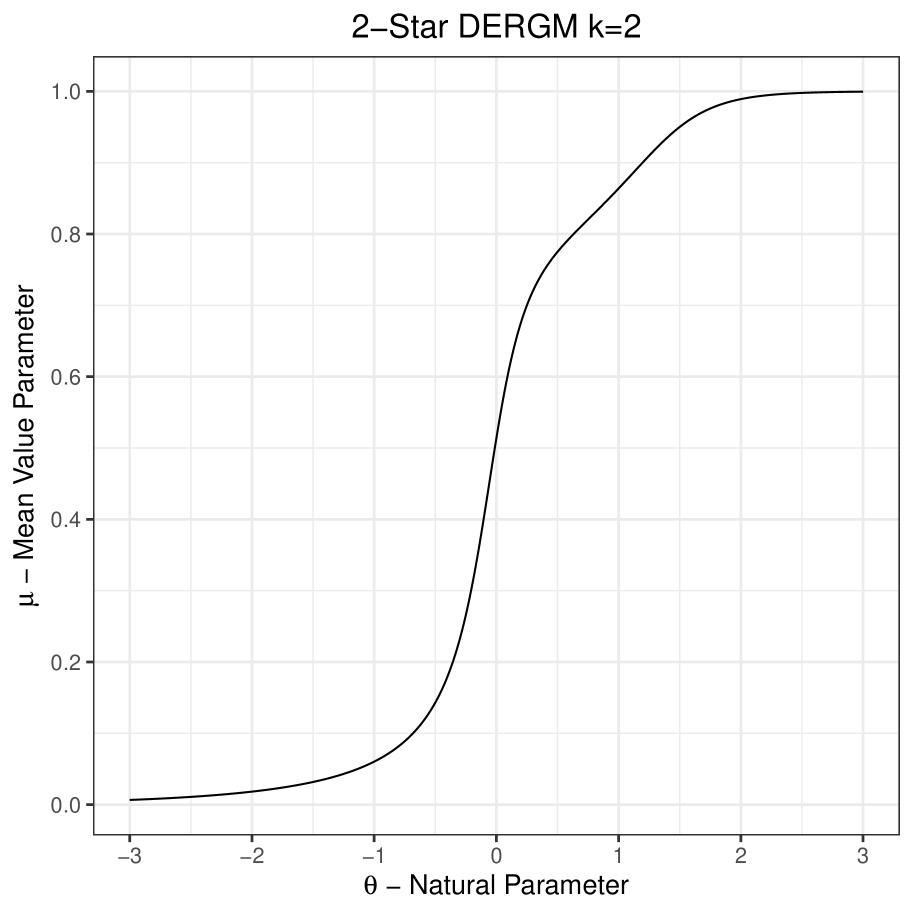
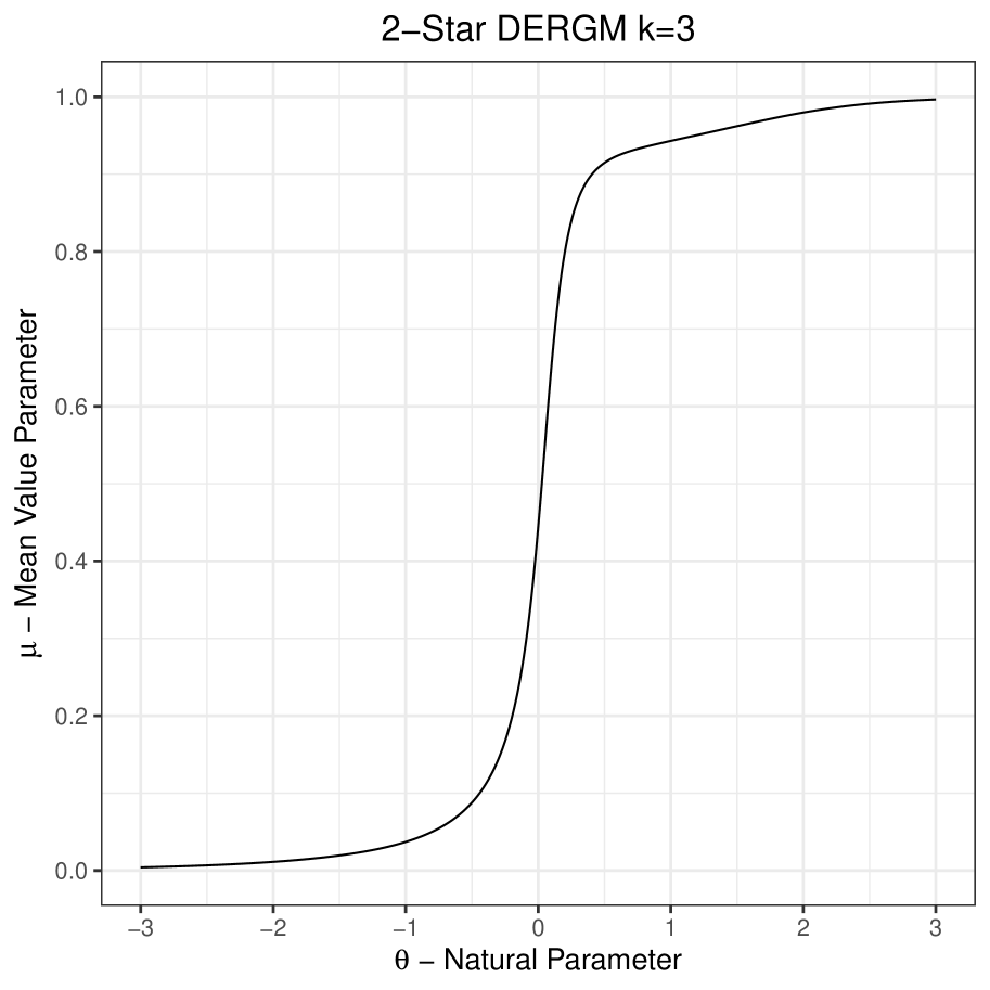
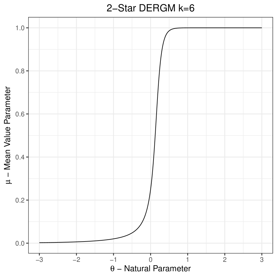
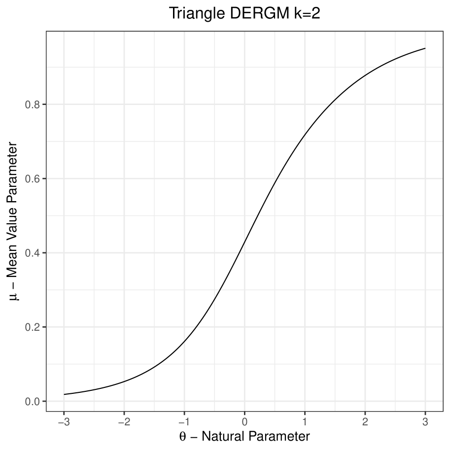
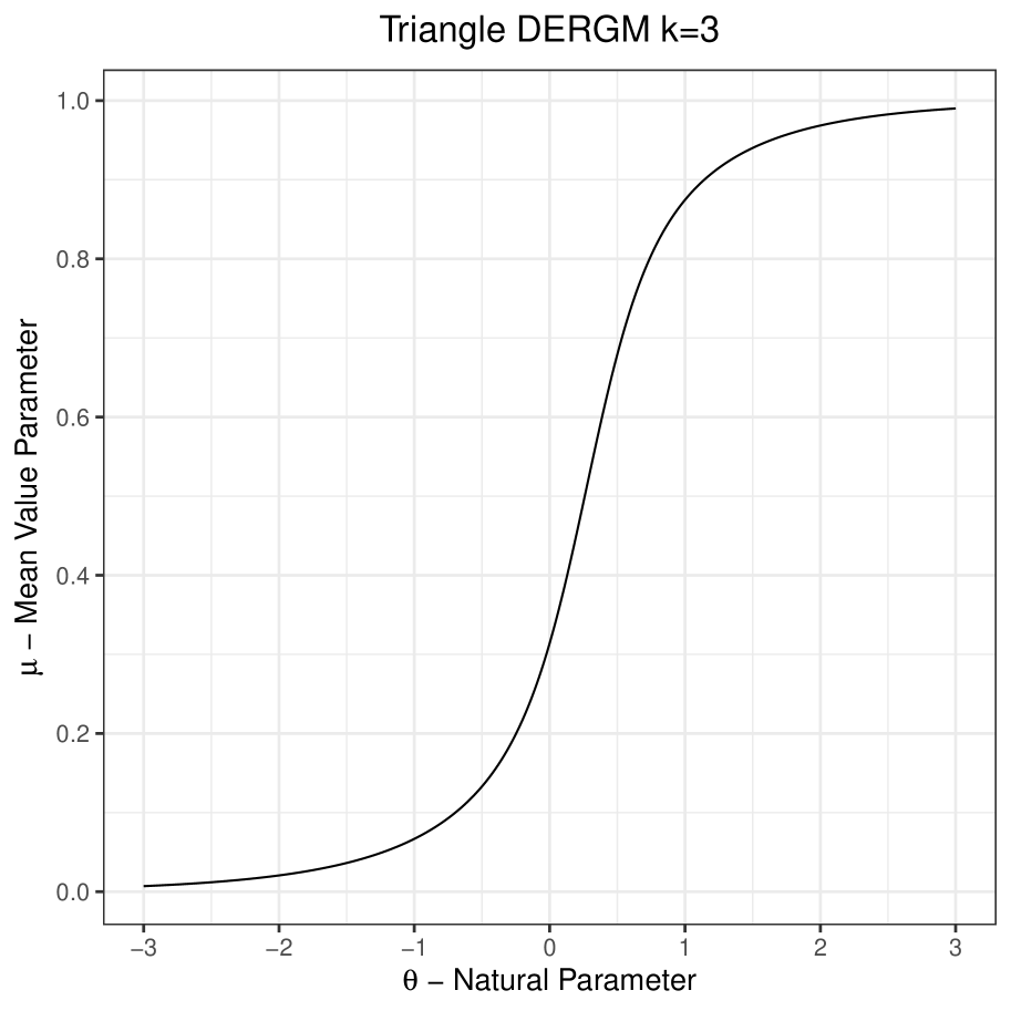
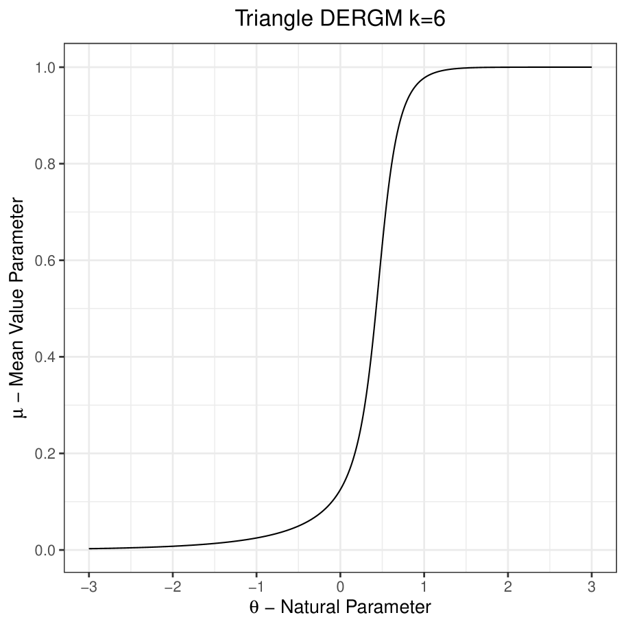
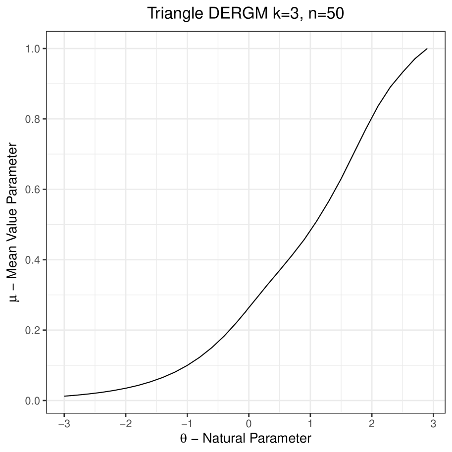
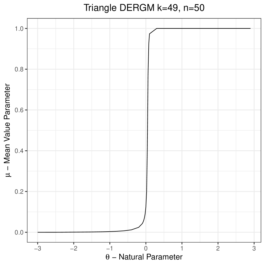
Let us focus on Figure 3(c). This figure shows the map between $\theta$ and $\mu_{k}(\theta)$ for the triangle-DERGM when $k=6$ and $n=7$, which is the same as the ERGM (since $k=6$ is the maximum possible, there is no support restriction). The plot shows that the mean value parameter is pushed to its corresponding boundaries for positive and negative values of $\theta$, i.e. for $\theta>0$, $\mu_{k}(\theta)$ is close to 1, and for $\theta<0$, $\mu_{k}(\theta)$ is close to 0. Moreover, for $\theta$ close to $0$, the mean value parameter is very sensitive to small changes in $\theta$. This is the classic model degeneracy and excessive sensitivity. On the other hand, if we consider Figures 3(a) and 3(b), we can see that if we restrict the support to $2$-degenerate graphs or $3$-degenerate graphs, the mean value map improves. Specifically, for $k=2$, Figure 3(a) shows that $\mu_{k}(\theta)$ is not pushed to its boundaries for positive or negative values of $\theta$, and has a small derivative near $\theta=0$. This shows that the model does not suffer from degeneracy and excessive sensitivity when $k$ is small. A similar conclusion holds for the $2$-star model shown in Figure 2. We also created such plots for $n=50$, for which we had to resort to MCMC sampling to estimate the mean value parameters, see Figure 4 for the triangle DERGM for $k=3$ and $k=50$. The results for this setting was the same as described here: For small values of $k$, the triangle and the two-star DERGM does not suffer from excessive sensitivity and model degeneracy.

(a) $n=50$, $k=3$

(b) $n=50,k=49$

Figure 4: Simulated plot of Mean value parameters vs Natural parameters, based on MCMC, for the triangle DERGM for $n=50$ and $k=3$ and $k=49$ respectively.

4.2 Existence of approximate MLE, the model polytope, and entropy

Consider first the issue of existence of the approximate MLE. Recall from Section 3.2 that in the MCMC-MLE estimation, the approximate MLE does not exist when the observed sufficient statistics lies outside of the convex hull of the sufficient statistics sampled from $\mathbb{P}_{\theta_{0}}$. In DERGMs, this is more likely to happen when the degeneracy parameter $k$ is large relative to the observed graph degeneracy.

As an example to illustrate this phenomenon, consider fitting the edge-triangle DERGM to Sampson monastery data Sampson, (1968), in particular, the time period T4, available at Batagelj & Mrvar, (2006) and Hunter et al., (2008a). In this data set, $n=18$ and observed graph degeneracy is $k=3$. Building on the correspondence between MLE non-existence and the model polytope from Rinaldo et al., (2009), we study the location of the observed edge-triangle vector with respect to estimated DERGM model polytopes for varying values of $k$. Recall that the model polytope for an exponential family model is the convex hull of all observable vectors of sufficient statistics. We estimate the DERGM polytopes as convex hulls of edge-triangle pairs of networks obtained by sampling graphs uniformly from the support $\mathcal{G}_{n,k}$, using Algorithm 2. Figure 5 shows the estimated model polytopes for different values of $k$, along with the relative location of the Sampson edge-triangle vector. When $k=3$, the observed sufficient statistic lies well in the relative interior of the sampled sufficient statistics. On the other hand, when $k=6$ and higher, the observed sufficient statistic lies well outside the convex hull.

(a) $n=18$, $k=3$

(b) $n=18$, $k=4$

(c) $n=18$, $k=5$

(d) $n=18$, $k=6$

Figure 5: Estimated edge-triangle DERGM model polytopes for increasing $k$, with $x$ marking the location of the observed sufficient statistic of the Sampson graph. Sample size is $100,000$ each; we have verified that the results do not change when sample size is increased to $1,000,000$. We do not plot the estimated polytopes for all other values of $k>6$, but the reader can rest assured that the observed value of the sufficient statistics of the Sampson graph only gets farther removed from the convex hull.

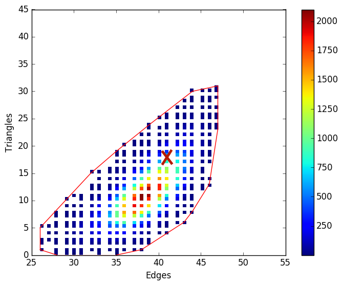
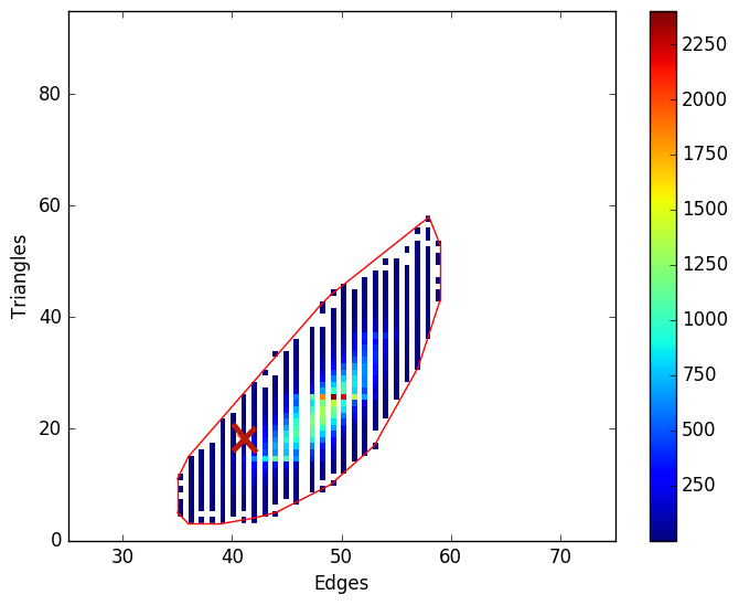
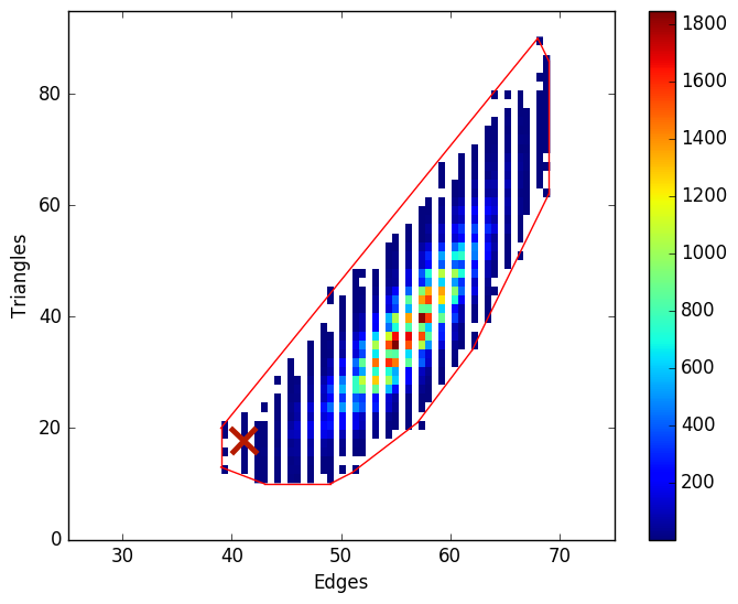
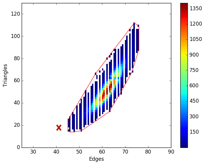
As $k$ increases, the observed edge-triangle count is progressively pushed out of the estimated polytope and becomes probabilistically less likely under the uniform distribution (blue corresponds to lower probability). This is because for larger $k$, the uniform sampler places more weight on edge-triangle counts of denser graphs, making more sparse edge-triangle counts such as those from Sampson graph probabilistically less likely to appear. Thus, for larger $k$, the observed edge-triangle count of the Sampson graph lies in the tails of the distribution induced by the uniform sampler. This in turn effects the MCMC-MLE as follows: For larger $k$, the observed sufficient statistic lies close to the boundary of the true model polytope, or as the figures show, outside the estimated polytope. Unless the MCMC algorithm finds a $\theta_{0}$ that generates graphs around the observed sufficient statistic, the approximate MLE will not exist. However, this is difficult, since as the observed sufficient statistic approaches the boundary, the number of network configurations corresponding to it becomes smaller. This concept can be formalized by measuring the entropy, discussed next.

Entropy.

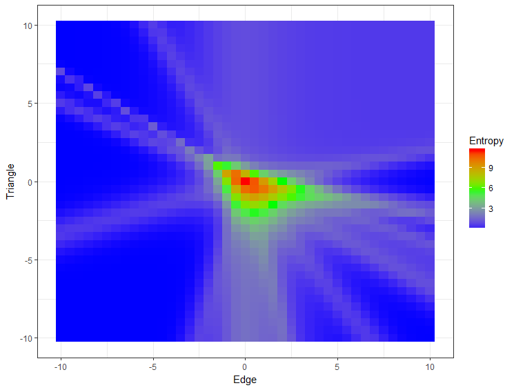
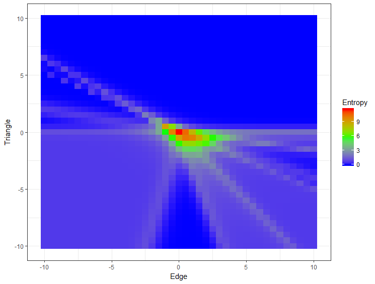
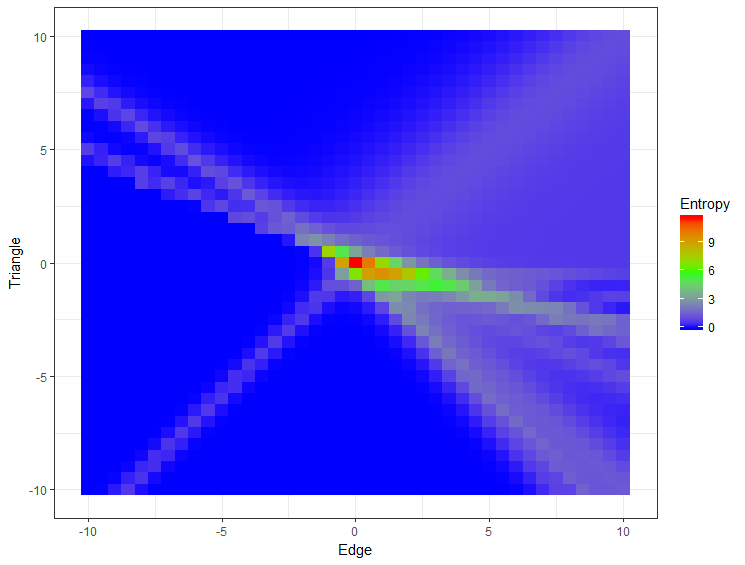
As explained in Rinaldo et al., (2009) (see Section 3.4 therein for details), the shape of the model polytope supports the argument that the full ERGM is ill-behaved. Specifically, they use Shanon’s entropy, which captures the degree to which the model concentrates its mass on network configurations associated with a relatively very small number of network statistics. The rationale is that degenerate models have large areas of low entropy. The correspondence between the model polytope and model degeneracy derived by Rinaldo et al. shows that the extremal rays of the normal fan of the model polytope correspond to directions of the ridges of Shanon’s entropy function where it converges to some fixed value. These extremal rays are outer-normals of the facets (in our case, edges) of the polytope; we see that as $k$ grows, the polytope becomes ‘flatter’ or, equivalently, the directions of the outer-normals of the edges on the lower hull get closer together, making the area of high entropy smaller. Although the exact plots are unavailable for the full ERGM on $n=18$, we know that for $n=9$ already the rays of normal fan concentrate in a small area of the plane implying that the model has low entropy and is degenerate for a vast majority of parameter values; cf.  (Rinaldo et al.,, 2009, Figure 4A). As the authors in the said article justify, we use the mean value parameters to illustrate this behavior, where it can be clearly seen.

In contrast, Figure 6 shows that the higher-entropy region is more ‘spread out’ across the parameter region for the DERGMs with smaller values of $k$. While one cannot, of course, conclude that the model is non-degenerate for all possible parameter values, it is clear that the size of the parameter space that correspond to degenerate regions is certainly less than in the full ERGM. Regarding the caveat that the Figures are also estimated and not exact, we are nevertheless confident in the results, because 1) the algorithm used is a uniform sampler of well-ordered graphs from the model support $\mathcal{G}_{n,k}$; and 2) the estimated polytope is not far off from the true model polytope: it is missing some extremal graphs that are probabilistically unlikely to be generated by the uniform sampler from the space of graphs $\mathcal{G}_{9}=\mathcal{G}_{9,8}$.

(a) $n=18$, $k=3$

(b) $n=18$, $k=4$

(c) $n=18$, $k=5$

Figure 6: Comparison of degenerate (low-entropy) regions in the mean-value parameter space for the edge-triangle DERGMs on $n=18$ and increasing $k$. Sample sizes are $100,000$. As $k$ increases, the high-entropy region becomes smaller.

4.3 The likelihood surface changes with $k$

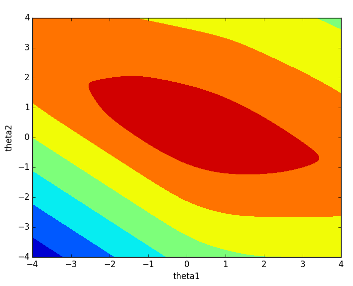
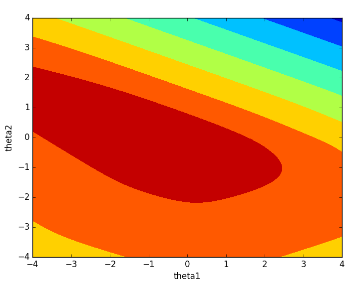
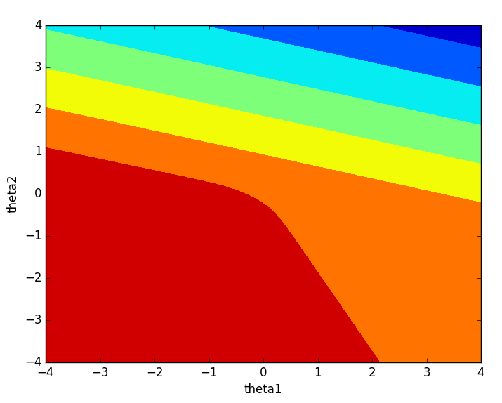
The shape of the estimated likelihood function changes as we change $k$. To illustrate this, we use the uniform sampler given in Algorithm 2 to sample graphs uniformly from the support of the full ERGM $\mathcal{G}_{n}=\mathcal{G}_{n,n-1}$ and $\mathcal{G}_{n,k}$ with $k<n-1$ for various DERGMs, and estimate the likelihood function using the sampled graphs for the Sampson network. Figure 7 shows the contours of the (estimated) likelihood function for various values of $\theta=(\theta_{1},\theta_{2})$. This figure uncovers an interesting trend: the likelihood surface becomes ‘flatter’ around the maximum value as $k$ grows, making it more difficult to find the maximum itself after a certain number of steps.

(a) $n=18$, $k=3$

(b) $n=18$, $k=4$

(c) $n=18$, $k=17$

Figure 7: Contour plots of the estimated edge-triangle DERGM likelihood functions for the Sampson network, for various values of $(\theta_{1},\theta_{2})$. Here, $n=18$ and $k=3,4,17$. Note that $k=17$ corresponds to the full ERGM. The estimated likelihood is based on an iid sample of $25,000$ graphs in $\mathcal{G}_{n,k}$.

5 Estimation and fitting DERGMs on real world data

In this section, we present the results of fitting DERGMs to some real world networks. These results were obtained by fitting the DERGMs using the MCMC-MLE estimation algorithm using the tie-no-tie procedure, and Hummel et al., (2012) step length algorithm to improve the estimation. The degeneracy parameter $k$ was set to its observed value.

5.1 Examples where DERGMs fit whereas ERGM fit fails to converge

We first start by showing three examples where the MCMC-MLE procedure fails to converge when fitting an edge-triangle ERGM, whereas it converges when using the edge-triangle DERGM with the degeneracy parameter set to the observed degeneracy. We consider three networks - an undirected version of the Sampson dataset, the Faux Mesa High network and the undirected version of ecoli network, from the ergm package in R. The summary statistics of these networks are given in Table 2. Note that we are not claiming that the edge-triangle DERGM is the best model for these data. Instead, the point is to illustrate that restricting the degeneracy has a direct impact on MCMC-MLE estimation.

Network	Nodes	Edges	Degeneracy
Sampson	18	41	3
Faux Mesa High	205	203	3
Ecoli	418	519	3

Table 2: Summary of Datasets used to fit the edge-triangle DERGMs

The Sampson network has $n=18$ nodes and $m=41$ edges, with an observed degeneracy $k=3$. The Faux Mesa High network has $205$ nodes and $203$ edges, and an observed degeneracy of $3$. The ecoli network has $n=423$ nodes, $m=519$ edges with a degeneracy $k=3$. Note that all the networks have a low observed degeneracy. In particular, the ecoli and the faux mesa high networks are very sparse since the degeneracy is very small in comparison to the number of nodes.

While fitting the edge-triangle ERGM to these networks, the MCMC-MLE combined with the step length procedure failed to converge due to model degeneracy; for a detailed study of this model’s degeneracy, see Rinaldo et al., (2009). Specifically, the Markov chain started sampling networks whose number of edges and triangles are very far from the observed network, indicating model degeneracy. On the other hand, there were no such issues when fitting the edge-triangle DERGM and the MCMC-MLE combined with the step length procedure converged. The estimated parameter for the edge-triangle DERGMs for these networks are given in Table 3. There are two sources of standard error here, one from the MCMC estimation and another corresponding to the MCMCMLE. The MCMCMLE standard errors are calculated by using an MCMC estimate of the inverse of the estimated fisher information matrix, as described in Hunter & Handcock, (2006).

Networks	Faux Mesa High	Sampson	Ecoli
edges	$-5.13^{***}$	$-1.62^{***}$	$-5.32^{***}$
	$(0.08)$	$(0.34)$	$(0.05)$
triangle	$2.62^{***}$	$0.36$	$(2.65)^{***}$
	$(0.10)$	$(0.34)$	$(0.16)$
AIC	2029.17	157.41	6210
BIC	2045.06	163.47	6229
${}^{***}p<0.001$

Table 3: Fitting the edge-triangle DERGM where the edge-triangle ERGM fit fails. The ^∗ denotes level of significance, based on the $p$-values. (The numbers in the parenthesis are the standard errors of the MCMCMLE.)

5.2 Examples when both ERGM and DERGM fit converges

We now consider cases where the MCMC-MLE procedure is able to fit both an ERGM and a DERGM to the same dataset. In these cases, we show that the parameter estimates obtained from both these models are very close to each other. We fit the edge-triangle DERGMs and ERGM to the florentine dataset. This dataset has $n=16$ vertices and $m=20$ edges, with a degeneracy parameter $k=2$. We fit DERGMs with increasing values of $k=2,3,\ldots,15$. Note that when $k=15$, the DERGM is equivalent to the edge-triangle ERGM. The parameter estimates are given in Table 4. This table shows that the edge parameter is more or less the same for all the DERGMs and ERGM. The parameter corresponding to the triangles varies, but is within the margin of the standard error.

Degeneracy	2	3	4	10	15
($k$)					(ERGM)
edges	$-1.672^{***}$	$-1.678^{***}$	$-1.675^{***}$	$-1.672^{***}$	$-1.667^{***}$
	$(0.392)$	$(0.362)$	$(0.352)$	$(0.346)$	$(0.351)$
triangle	$0.410$	$0.172$	$0.167$	$0.152$	$0.146$
	$(0.731)$	$(0.595)$	$(0.580)$	$(0.572)$	$(0.596)$
AIC	111.786	112.058	112.073	112.090	112.071
BIC	117.361	117.633	117.648	117.665	117.646
Log Likelihood	-53.893	-54.029	-54.036	-54.045	-54.035
${}^{***}p<0.001$

Table 4: Fitting DERGM and ERGM to the Florentine data. The ^∗ denotes level of significance, based on the $p$-values. (The numbers in the parenthesis are the standard errors of the MCMCMLE.)

6 Uniform samplers for $\mathcal{G}_{n,k}$

The main contribution of this section is the development of a fast uniform sampler of the space of well-ordered graphs in $\mathcal{G}_{n,k}$, contained in Section 6.1, which has been used throughout Section 4 in simulations, most prominently for estimated polytope plots. We discuss the basis of the algorithm and the updates we made to make it scalable. This algorithm can be used stand-alone for Monte Carlo sampling for DERGM estimation, specifically in the case when non-well-ordered graphs are not of interest. On the other hand, it can also be used in combination with a non-well-ordered sampler to create a stratified sampler for all graphs of $\mathcal{G}_{n,k}$ when needed; below, we discuss how in some cases the stratified sampler effectively reduces to the well-ordered one. Finally, if the observed graph is well outside the convex hull of sampled graphs, one may wish to use a fast importance MCMC sampler, in conjunction with the uniform sampler from Section 6.1 to create an umbrella sampler on $\mathcal{G}_{n,k}$. The umbrella sampler converged quickly in simulations, but we omit those results here as they were not necessary for the data sets we analyze.

6.1 A uniform sampler for well-ordered graphs from $\mathcal{G}_{n,k}$

In (Bauer et al.,, 2010, Algorithm 1), the authors derive a uniform sampler for the set of well-ordered graphs in $\mathcal{G}_{n,k}$. A well-ordered graph is one in which the node labels are ordered so that no vertex has more than $k$ neighbors with a higher label.

Using this algorithm as a starting point, we make several key changes to ensure that their algorithm is computationally efficient: we convert their algorithm from a recursive one to an iterative one. By doing this, we eliminate many complexity problems inherent in the original algorithm. Specifically, the iterative version eliminates stack overflow issues for large graphs, as well as greatly reduces the execution time of generating a graph.

Let us take a closer look at the following algorithm, based on (Bauer et al.,, 2010, Algorithm 1), which we improved and updated to a scalable version.

input : $n$, the number of nodes,

$k$, maximum graph degeneracy.

output : $g$, a graph in $\mathcal{G}_{n,k}$ in which every vertex $i$ has no more than $\geq k$ neighbors in the set $\{i+1,\dots,n\}$.

1 for $i=1$ to $n$ do

2      $d_{i}\sim$ restrictedBinomial$(n-i,$ min$(n-i,k))$

3       if $i=n$ then

4            $V=V\cup\{n\}$

5 end for

6for $i=n$ to 1 do

7      $T=\{\}$

8       $P=V$

9       $a=|P|$

10       for $j=0$ to $d_{i}-1$ do

11             $m\sim$ Uniform$(0,a-j)$

12             $T=T\cup\{(i,P_{m})\}$

13             $P_{m}=P_{a-j-1}$

14       end for

15      $V=V\cup\{i\}$

16       $E=E\cup\{T\}$

17 end for

18$G=\{V,E\}$

return G

Algorithm 2 Generate a well-ordered $g$ from $\mathcal{G}_{n,k}$ uniformly.

The algorithm was originally formulated using recursion, which we emulate using two for-loops. The first for-loop populates a list of degrees where each index of the list corresponds to the respective vertex label. The degrees for each vertex are generated using a restricted binomial distribution. Instead of utilizing the cumulative distribution and using binary search to obtain values as suggested by the original paper, we opt to use the probability density function and store the values in a list data structure, reducing the complexity of obtaining the degree values. When the loop reaches the very last vertex, we add that vertex to the working vertex set. For each iteration in the second for-loop, a temporary copy of the current working vertex set is created. We then uniformly generate $d_{i}$ indices to sample without replacement from the vertex set copy, and use these samples for the edge set of the current vertex. It is obvious that this sample is uniformly generated, complying with the original algorithm.

For a benchmark, we tested the original recursive version (including generating all possible combinations) and the new iterative version on a machine with the following specifications: Intel Core i7-4790K CPU @ 4.00 GHz, 8 GB DDR3 RAM, Arch Linux x64, with the results shown in Table 5. The results clearly indicate that the scalable version is superior in regards to time complexity.

$(n,k)$	Original Recursive Algorithm	Our Iterative Version
	(Bauer et al.,, 2010, Algorithm 1)	Algorithm 2
$(50,8)$	$3.96$ seconds	$0.03$ seconds
$(800,2)$	Stack Overflow	$0.51$ seconds
$(3000,2)$	Stack Overflow	$1.90$ seconds

Table 5: Run times of the uniform samplers.

In some applications, it may be desirable to further restrict the sample space of the model by restricting the total number of edges of the graph, or use such a restriction for stratified sampling of $\mathcal{G}_{n,k}$. To that end, let $\mathcal{G}_{n,m,k}$ be the set of graphs on $n$ nodes and degeneracy $k$ with exactly $m$ edges. (Bauer et al.,, 2010, Algorithm 2) offer an algorithm for uniform sampling of $\mathcal{G}_{n,m,k}$, however, it was not implemented due to the complexity of step $3$ that the authors suggest be implemented using Equation (2.7) in Bauer et al., (2010). Pre-computation of degrees proved nearly impossible in practice for several reasons. The recursive nature of calculating the cardinality for possible graphs of given vertices, edges, and degeneracy yielded very inefficient computations in which the run time of each computation was longer than trying to generate whole graphs by other means. While we were able to alleviate this issue somewhat by utilizing a dynamic programming approach with memoization, even for semi-sparse, average size graphs, numerical overflow occurred, which rendered the speed increase fruitless. Instead, we opt to use (Bauer et al.,, 2010, Algorithm 3), which is a non-uniform but fast sampler of $\mathcal{G}_{n,m,k}$. Our implementation of this algorithm, outlined in Algorithm 3, stays true to the pseudo-code given in the original paper, with the only alteration being utilizing the same approach to uniform selection as in our implementation of Algorithm 2.

input : $n$, the number of nodes,

$m$, the number of edges,

$k$, maximum graph degeneracy.

output : $g$, a graph in $\in\mathcal{G}_{n,k}$ with $m$ edges in which every vertex $i$ has no more than $\geq k$ neighbors in the set $\{i+1,\dots,n\}$.

1 $C={1,...,v_{n-1}}$

2 for $i=1$ to $m$ do

3      $j\sim$ Uniform$(0,|C|)$

4       $d_{j}=d_{j}+1$

5       if $d_{j}=$ min$(n-v_{j},k)$ then

6            $C$ \$\{v_{j}\}$

7 end for

8for $i=1$ to $n-1$ do

9      $T=\{\}$

10       $P=V$

11       $a=|P|$

12       for $j=0$ to $d_{i}-1$ do

13             $m\sim$ Uniform$(0,a-j)$

14             $T=T\cup\{(i,P_{m})\}$

15             $P_{m}=P_{a-j-1}$

16       end for

17      $V=V\cup\{i\}$

18       $E=E\cup\{T\}$

19 end for

20$G=\{V,E\}$

return G

Algorithm 3 Generate a well-ordered $g$ from $\mathcal{G}_{n,m,k}$ non-uniformly.

6.2 Stratified sampling of $\mathcal{G}_{n,k}$ to include non-well-ordered graphs if needed

Another issue with (Bauer et al.,, 2010, Algo.1) is that it generates only so-called ‘well-ordered’ graphs in $\mathcal{G}_{n,k}$. This misses a part of graphs in the support of our model. To remedy this issue, we classify all missing graphs and produce them via stratified sampling with two strata. Specifically, Algorithm 2 is used to sample from the set of well-ordered graphs in $\mathcal{G}_{n,k}$, while Algorithm 4, described below, is used to generate non-well-ordered graphs in $\mathcal{G}_{n,k}$. Let $n_{1}$ and $n_{2}$ be the number of well-ordered and non-well-ordered graphs, respectively. The formula for $n_{1}$ is provided in Bauer et al., (2010) under the notation $D_{n}^{(k)}$, while $n_{2}$ is studied below. To the best of our knowledge, the literature does not provide a good estimate of the number $n_{1}$ of well-ordered $k$-degenerate graphs compared to the total number of $k$-degenerate graphs. Although we derived a lower bound on the total number of $k$-degenerate graphs ($\Omega(n\log n)$) in Theorem 1, in this section we study the ratio of $n_{1}$ and $n_{2}$ further, which is needed from an algorithmic point of view. It should be noted that, in practice, the uniform sampler from Section 6.1 may only be omitting a tiny fraction of graphs in the support of the DERGM; this situation is described in detail at the end of this Section. Therefore, the reader interested in applications more than in theory behind the algorithms that may not be necessary in practice may skip the remainder of this technical section.

A graph $g\in\mathcal{G}_{n,k}$ is not well-ordered if there exists at least one vertex $j$ with at least $k+1$ neighbors in the set $\{j+1,\dots,n\}$. Among all such vertices with too many big neighbors, let $k+c$ be the minimum such number of big neighbors, and let $i$ be the index of the smallest vertex that has $k+c$ big neighbors. We construct non-well-ordered graphs and use them to estimate $n_{1}$ by going through possible cases for the values of $c$ and $i$. For each case $c=1,\dots,n-k-1$, some vertex $i$ has $k+c$ neighbors in the set $\{i+1,\dots,n\}$. For each of the cases, the vertex $i$ can be chosen from the set $\{1,\dots,n-(k+c)\}$. Note that these $k+c$ neighbors of $i$ can be connected in any arbitrary way, as long as the entire graph is in $\mathcal{G}_{n,k}$. Thus, we proceed as follows: construct a random graph $h$ on $k+c$ vertices whose labels are in the set $\{i+1,\dots,n\}$. Then, construct a suspension $g$ over $h$ using vertex $i$, that is, ensure that $i$ is connected to all $k+c$ vertices of $h$. Finally, the vertices $\{1,\dots,i\}$ can be connected in any way such that, by minimality of $i$, the resulting subgraph on $\{1,\dots,i\}$ is well-ordered and, additionally, each vertex in the set $\{1,\dots,i\}$ can have at most $k$ neighbors in the vertex set $\{i+1,\dots,n\}$. The construction is outlined in Algorithm 4.

input : $n$, the number of nodes,

$k$, maximum graph degeneracy.

output : $g$, a graph in $\in\mathcal{G}_{n,k}$ (or $\mathcal{G}_{n,d}$ with $d>k$, unfortunately) in which there is a vertex $i$ that has $\geq k+1$ neighbors in the set $\{i+1,\dots,n\}$.

1 Pick $c\in\{1,\dots,n-k-1\}$.

2Pick $i\in\{1,\dots,n-(k+c)\}$.

3Use Algorithm 2 to sample $\tilde{h}\in\mathcal{G}_{k+c,k+c-1}$; repeat until $degen(\tilde{h})\leq k$.

4 Choose (uniformly) a subset of $k+c$ vertex labels from the set of legal vertex labels $\{i+1,\dots,n\}$.

5 Let $h$ be the graph obtained from $\tilde{h}$ by replacing the labels $1,\dots,k$ by those selected on Line 4.

6 Create the suspension graph $g$ over $h$ by adding to $h$ edges $\{i,x\}$ for all $x\in V(h)$.

7 Connect vertices $\{1,\dots,i\}$ by constructing any well-ordered graph from $\mathcal{G}_{i,k}$.

8 Connect any of the vertices $\{1,\dots,i\}$ to at most $k$ vertices in the set $\{i+1,\dots,n\}$.

9 Output $g$ if $degen(g)\leq k$; otherwise return to Step 4.

10

Algorithm 4 Generate a non-well-ordered $g$ from $\mathcal{G}_{n,k}$

There are ${n-i\choose k+c}$ ways to choose the neighbors of the vertex $i$ on Line 4 and for each choice of neighbors there are $2^{k+c\choose 2}$ graphs $\tilde{h}$ generated on Line 4. There are $D^{(k)}_{i}$ well-ordered graphs on Line 4 and $i\sum_{p=1}^{k}{n-i\choose p}$ graphs on Line 4. Thus, Algorithm 4 constructs the following number of graphs $g$:

$$\underbrace{\sum_{i=1}^{n-(k+1)}\underbrace{{n-i\choose k+1}}_{\mbox{Line~{}\ref{line:vtx.shift}}}\cdot\underbrace{2^{k+1\choose 2}}_{\mbox{Line~{}\ref{line:htilde}}}\cdot\underbrace{D_{i}^{(k)}}_{\mbox{Line~{}\ref{line:connect1thrui}}}\cdot\underbrace{i\sum_{p=1}^{k}{n-i\choose p}}_{\mbox{Line~{}\ref{line:connect1thruiToBig}}}}_{c=1}$$

$$+\underbrace{\sum_{i=1}^{n-(k+2)}{n-i\choose k+2}\cdot 2^{k+2\choose 2}\cdot D_{i}^{(k)}\cdot i\sum_{p=1}^{k}{n-i\choose p}+\dots}_{c=2}$$

$$\dots+\underbrace{\sum_{i=1}^{n-(k+n-k-1)}{n-i\choose n-1}\cdot 2^{n-1\choose 2}\cdot D_{i}^{(k)}\cdot i\sum_{p=1}^{k}{n-i\choose p}}_{c=n-k-1}$$ (8)

$$=2^{k+1\choose 2}\cdot\sum_{i=1}^{n-(k+1)}{n-i\choose k+1}\cdot D_{i}^{(k)}\cdot i\sum_{p=1}^{k}{n-i\choose p}$$

$$+2^{k+2\choose 2}\cdot\sum_{i=1}^{n-(k+2)}{n-i\choose k+2}\cdot D_{i}^{(k)}\cdot i\sum_{p=1}^{k}{n-i\choose p}+\dots$$

$$\dots+2^{n-1\choose 2}\cdot{n-1\choose n-1}\cdot D_{i}^{(k)}\cdot i\sum_{p=1}^{k}{n-i\choose p},$$ (9)

where each of the $n-k-1$ summands corresponds to one of the cases $c$.

Note that Equation (9) is an upper bound on $n_{2}$, since it counts all graphs $g$ constructed by Algorithm 4. It is also a strict upper bound on the number of graphs $g$ actually returned by the algorithm, since it counts those graphs whose degeneracy happens to be strictly larger than $k$.

Equation (9) counts all graphs on $k+c$ nodes, $2^{k+c\choose 2}$, constructed in Step 4. Surely, a better count can be obtained by replacing $2^{k+c\choose 2}$ by

$$2^{k+c\choose 2}-\#\{\mbox{well-ordered graphs on $k+c$ vertices of degeneracy}>k\}.$$

Doing this replacement in the equation is, crucially, still an upper bound on $n_{2}$ (since the well-ordered graphs of degeneracy larger than $k$ certainly do not contribute to any non-well-ordered graphs of degeneracy at most $k$). Since

$$\#\{\mbox{well-ordered graphs on $k+c$ nodes of degeneracy}>k\}$$

$$= \#\{\mbox{all well-ordered graphs on $k+c$ nodes except those of degereacy}\leq k\}$$

$$= D^{(k+c-1)}_{k+c}-D^{(k)}_{k+c},$$

the following is a better upper bound on the number of graphs we wish to keep from Algorithm 4 and thus also an upper bound on $n_{2}$:

$$\sum_{i=1}^{n-(k+1)}{n-i\choose k+1} \cdot\left(2^{k+1\choose 2}-\left(D^{(k+1-1)}_{k+1}-D^{(k)}_{k+1}\right)\right)\cdot D_{i}^{(k)}\cdot i\sum_{p=1}^{k}{n-i\choose p}+$$

$$\sum_{i=1}^{n-(k+2)}{n-i\choose k+2} \cdot\left(2^{k+2\choose 2}-\left(D^{(k+2-1)}_{k+2}-D^{(k)}_{k+2}\right)\right)\cdot D_{i}^{(k)}\cdot i\sum_{p=1}^{k}{n-i\choose p}+\dots$$

$$\dots+{n-1\choose n-1} \cdot\underbrace{\left(2^{n-1\choose 2}-\left(D^{(n-1-1)}_{n-1}-D^{(k)}_{n-1}\right)\right)}_{\mbox{Line~{}\ref{line:htilde} minus well-ordered of degen}>k}\cdot D_{i}^{(k)}\cdot i\sum_{p=1}^{k}{n-i\choose p}.$$ (10)

Let

$$t_{true}=\log n_{1}/(n_{1}+n_{2})$$

be the true threshold used to divide the sample in two strata and define

$$t_{estimated}=\log n_{1}/(n_{1}+\eqref{eq:BETTERNumGraphsFromNWOalgorithmWeAreKeeping}).$$

Given that $\eqref{eq:BETTERNumGraphsFromNWOalgorithmWeAreKeeping}>n_{2}$, $t_{estimated}<t_{true}\leq 0$. Therefore we take the following approach: 1) compute the threshold $t_{estimated}$ for the fixed n and k for which we wish to run the current simulation. 2) If $t_{estimated}$ is close to $0$, then that forces $t_{true}$ to be close to $0$, which in turn means that there is a very, very small number of non-well-ordered graphs for that choice of $n$ and $k$ and therefore the stratified sampler essentially reduces to sampling well-ordered graphs only.

Of course, if $t_{estimated}$ is not relatively close to $0$, then for those values of $n$ and $k$, while it is possible that $t_{true}$ is close to $0$, one should implement both the well-ordered and non-well-ordered algorithm. Falling back on the well-ordered algorithm is equivalent to using an approximate sampler in practice. The users may additionally prefer to replace Algorithm 4 by instead permuting the vertices of the output of Algorithm 2, allowing it to reach the entire sample space $\mathcal{G}_{n,k}$ in another way.

Remark 7.

In practice, if the model’s sufficient statistics are subgraph counts (or if the distribution is exchangeable), well-ordering does not pose a restriction, because in the uniform sampling using MC in estimating the MLE, only the values of the sufficient statistics of the sampled graphs are used. These are oblivious to vertex labels, so ordering is irrelevant.

7 Discussion

In this paper, we introduced a general modification of exponential family random graph models that solves some of the model degeneracy issues. This modification amounts to a support restriction, by conditioning on the observed network’s graph-degeneracy, which is a measure of sparsity that is weaker than imposing an upper bound on node degrees. The resulting model class, which we name degeneracy-restricted or DERGMs, does not suffer from the same estimation issues as the usual ERGMs. The proposed support restriction is interpretable as a weak sparsity constraint, it respects most real-world network data, and it provably does not eliminate a large part of the support of the full ERGM, while improving model behavior. Specifically, we show that DERGMs with smaller graph degeneracy parameter $k$ induce stable sufficient statistics, and we also show that such a stable behavior implies non-degeneracy of the model. Using simulations, we also show that DERGMs with small values of $k$ have a better-behaved simulated likelihood (i.e., more steep around the maximum) and the simulated model polytope spreads more mass around realistic graphs by eliminating very low-probability extreme graphs. This also makes MCMC algorithms to approximate the likelihood more stable, thus improving the MCMC-MLE estimation.

The particular example of the edge-triangle DERGM presented here is a good illustration of the general DERGM behavior. It is a natural choice of the running example, given the recent work by Rinaldo et al., (2009) that studies its degenerate behavior in detail. The general framework presented, however, applies to any ERGM; a good overview of many of the popular classes being offered in Goldenberg et al., (2009). Recent work on the shell-distribution ERGM Karwa et al., (2017) introduces a limited version of the current contribution: it is an example of an ERGM with similarly restricted support and gives direct motivation for the study of DERGMs in general. However, there, the model support was not $\mathcal{G}_{n,k}$ for fixed $n$ and $k$, but rather $\mathcal{G}_{n,k}\setminus\mathcal{G}_{n,k-1}$ - networks with degeneracy exactly $k$. Here were propose to use networks of degeneracy at most $k$, to enlarge the model support, and offer greater flexibility in modeling. Our contributions indicate that DERGMs may offer a feasible and interpretable modification of ERGMs, a powerful and flexible model class.

Extending the approach presented herein to directed graphs is one of the directions of future work. The notion of $k$-degeneracy as defined here applies only to undirected graphs, however it has been extended to directed graphs recently in Giatsidis et al., (2011). Another direction of future is to develop a distributed version of Algorithm 2. While we did run the current implementation in parallel, it can further be improved to run on a cluster. The current implementation scales very well to hundreds of nodes and with the additional step it should perform just as well on thousands.

References

- Bajić, (2016) Bajić, Denis. (2016). Dergms: Supplementary material on GitHub. https://github.com/dbajic/degen.
- Bannister et al., (2014) Bannister, Michael J., Devanny, William E., & Eppstein, David. (2014). ERGMs are hard. Preprint arXiv:1412.1787 [cs.DS].
- Barndorff-Nielsen, (2014) Barndorff-Nielsen, Ole. (2014). Information and exponential families in statistical theory. John Wiley & Sons.
- Batagelj & Mrvar, (2006) Batagelj, Vladimir, & Mrvar, Andrej. (2006). Pajek datasets. http://vlado.fmf.uni-lj.si/pub/networks/data/.
- Batagelj & Zaversnik, (2003) Batagelj, Vladimir, & Zaversnik, Matjaz. (2003). An o (m) algorithm for cores decomposition of networks. arxiv preprint cs/0310049.
- Bauer et al., (2010) Bauer, Reinhard, Krug, Marcus, & Wagner, Dorothea. (2010). Enumerating and generating labeled -degenerate graphs. Proceedings of the seventh workshop on analytic algorithmics and combinatorics (analco).
- Caimo & Friel, (2011) Caimo, Alberto, & Friel, Nial. (2011). Bayesian inference for exponential random graph models. Social networks, 33(1), 41–55.
- Chatterjee & Diaconis, (2013) Chatterjee, Sourav, & Diaconis, Persi. (2013). Estimating and understanding exponential random graph models. Annals of statistics, 41(5), 2428–2461.
- Engström & Norén, (2011) Engström, Alexander, & Norén, Patrik. (2011). Polytopes from subgraph statistics. Discrete mathematics and theoretical computer science.
- Fellows & Handcock, (2017) Fellows, Ian, & Handcock, Mark. (2017). Removing phase transitions from gibbs measures. Pages 289–297 of: Artificial intelligence and statistics.
- Frank & Strauss, (1986) Frank, Ove, & Strauss, David. (1986). Markov graphs. Journal of the american statistical association, 81(395), 832–842.
- Geyer & Thompson, (1992) Geyer, Charles J, & Thompson, Elizabeth A. (1992). Constrained monte carlo maximum likelihood for dependent data. Journal of the royal statistical society. series b (methodological), 657–699.
- Giatsidis et al., (2011) Giatsidis, Christos, Thilikos, Dimitrios M., & Vazirgiannis, Michalis. (2011). D-cores: Measuring collaboration of directed graphs based on degeneracy. Ieee 11th international conference on data mining.
- Goldenberg et al., (2009) Goldenberg, Anna, Zheng, Alice X., Fienberg, Stephen E., & Airoldi, Edoardo M. (2009). A survey of statistical network models. Foundations and trends in machine learning, 2(2), 129–233.
- Goodreau et al., (2009) Goodreau, Steven M, Kitts, James A, & Morris, Martina. (2009). Birds of a feather, or friend of a friend? using exponential random graph models to investigate adolescent social networks*. Demography, 46(1), 103–125.
- Handcock, (2003) Handcock, M. S. (2003). Assessing degeneracy in statistical models of social networks. Center for statistics and the social sciences, university of washington, working paper no. 39.
- Horvát et al., (2015) Horvát, Szabolcs, Czabarka, Éva, & Toroczkai, Zoltán. (2015). Reducing degeneracy in maximum entropy models of networks. Physical review letters, 114(15), 158701.
- Hummel et al., (2012) Hummel, Ruth M, Hunter, David R, & Handcock, Mark S. (2012). Improving simulation-based algorithms for fitting ergms. Journal of computational and graphical statistics, 21(4), 920–939.
- Hunter & Handcock, (2006) Hunter, David R, & Handcock, Mark S. (2006). Inference in curved exponential family models for networks. Journal of computational and graphical statistics, 15(3), 565–583.
- Hunter et al., (2008a) Hunter, David R, Handcock, Mark S, Butts, Carter T, Goodreau, Steven M, & Morris, Martina. (2008a). ergm: A package to fit, simulate and diagnose exponential-family models for networks. Journal of statistical software, 24(3), URL http://www.jstatsoft.org/v24/i03.
- Hunter et al., (2008b) Hunter, David R, Goodreau, Steven M, & Handcock, Mark S. (2008b). Goodness of fit of social network models. Journal of the american statistical association, 103(481), 248–258.
- Hunter et al., (2012) Hunter, David R, Krivitsky, Pavel N, & Schweinberger, Michael. (2012). Computational statistical methods for social network models. Journal of computational and graphical statistics, 21(4), 856–882.
- Karwa & Slavković, (2016) Karwa, Vishesh, & Slavković, Aleksandra. (2016). Inference using noisy degrees: Differentially private -model and synthetic graphs. The annals of statistics, 44(1), 87–112.
- Karwa et al., (2017) Karwa, Vishesh, Pelsmajer, Michael J., Petrović, Sonja, Stasi, Despina, & Wilburne, Dane. (2017). Statistical models for cores decomposition of an undirected random graph. Electronic journal of statistics, 11(1), 1949–1982. Preprint, arXiv:1410.7357 [math.ST].
- Kolaczyk & Krivitsky, (2015) Kolaczyk, Eric D, & Krivitsky, Pavel N. (2015). On the question of effective sample size in network modeling: An asymptotic inquiry. Statistical science: a review journal of the Institute of Mathematical Statistics, 30(2), 184.
- Krivitsky, (2012) Krivitsky, Pavel N. (2012). Exponential-family random graph models for valued networks. Electronic journal of statistics, 6(none), 1100 – 1128.
- Krivitsky et al., (2011) Krivitsky, Pavel N, Handcock, Mark S, & Morris, Martina. (2011). Adjusting for network size and composition effects in exponential-family random graph models. Statistical methodology, 8(4), 319–339.
- Lauritzen et al., (2018) Lauritzen, Steffen, Rinaldo, Alessandro, & Sadeghi, Kayvan. (2018). Random networks, graphical models and exchangeability. Journal of the Royal Statistical Society: Series B (Statistical Methodology), 80(3), 481–508.
- Lick & White, (1970) Lick, Don R, & White, Arthur T. (1970). k-degenerate graphs. Canadian j. of mathematics, 22, 1082–1096.
- Rinaldo et al., (2009) Rinaldo, Alessandro, Fienberg, Stephen E, & Zhou, Yi. (2009). On the geometry of discrete exponential families with application to exponential random graph models. Electronic journal of statistics, 3, 446–484.
- Rinaldo et al., (2013) Rinaldo, Alessandro, Petrović, Sonja, & Fienberg, Stephen E. (2013). Maximum lilkelihood estimation in the -model. The annals of statistics, 41(3), 1085–1110.
- Robbins & Monro, (1985) Robbins, Herbert, & Monro, Sutton. (1985). A stochastic approximation method. Pages 102–109 of: Herbert robbins selected papers. Springer.
- Sampson, (1968) Sampson, Samuel F. (1968). A novitiate in a period of change: An experimental and case study of relationships. Ph.D. thesis, Department of Sociology, Cornell University.
- Saul & Filkov, (2007) Saul, Zachary M, & Filkov, Vladimir. (2007). Exploring biological network structure using exponential random graph models. Bioinformatics, 23(19), 2604–2611.
- Schweinberger, (2011) Schweinberger, Michael. (2011). Instability, sensitivity, and degeneracy of discrete exponential families. Journal of the American Statistical Association, 106(496), 1361–1370.
- Schweinberger & Handcock, (2015) Schweinberger, Michael, & Handcock, Mark S. (2015). Local dependence in random graph models: characterization, properties and statistical inference. Journal of the royal statistical society: Series b (statistical methodology), 77(3), 647–676.
- Seidman, (1983) Seidman, Stephen B. (1983). Network structure and minimum degree. Social networks, 5(3), 269–287.
- Snijders, (2002) Snijders, Tom AB. (2002). Markov chain monte carlo estimation of exponential random graph models. Journal of social structure, 3(2), 1–40.
- Snijders et al., (2006) Snijders, Tom AB, Pattison, Philippa E, Robins, Garry L, & Handcock, Mark S. (2006). New specifications for exponential random graph models. Sociological methodology, 36(1), 99–153.
- Thiemichen & Kauermann, (2017) Thiemichen, Stephanie, & Kauermann, Goeran. (2017). Stable exponential random graph models with non-parametric components for large dense networks. Social networks, 49, 67–80.
- Yin et al., (2016) Yin, Mei, Rinaldo, Alessandro, Fadnavis, Sukhada, et al. . (2016). Asymptotic quantization of exponential random graphs. The annals of applied probability, 26(6), 3251–3285.