Effects of tidal gravitational fields in clustering dark energy models
Abstract
We extend a previous work by Reischke et al., 2016 by studying the effects of tidal shear on clustering dark energy models within the framework of the extended spherical collapse model and using the Zel’dovich approximation. As in previous works on clustering dark energy, we assumed a vanishing effective sound speed describing the perturbations in dark energy models. To be self-consistent, our treatment is valid only on linear scales since we do not intend to introduce any heuristic models. This approach makes the linear overdensity mass dependent and similarly to the case of smooth dark energy, its effects are predominant at small masses and redshifts. Tidal shear has effects of the order of percent or less, regardless of the model and preserves a well known feature of clustering dark energy: When dark energy perturbations are included, the models resemble better the CDM evolution of perturbations. We also showed that effects on the comoving number density of halos are small and qualitatively and quantitatively in agreement with what previously found for smooth dark energy models.
keywords:
Cosmology: theory - dark energy; Methods: analytical1 Introduction
A wealth of data accumulated over the last two decades (Riess et al., 1998; Perlmutter et al., 1999; Cole et al., 2005; Planck Collaboration XIII, 2016) strongly hints to the conclusion that the expansion of the Universe is currently accelerated and its origin represents one of the largest challenges and open questions in both physics and cosmology. The simplest explanation is the cosmological constant , which, so far, is very consistent with the data (Planck Collaboration XIII, 2016; Planck Collaboration XIV, 2016). Despite this agreement, a conclusive answer is still lacking and to refuse or confirm the standard cosmological model, dubbed CDM model, where is the cosmological constant responsible for the accelerated expansion and CDM represents the cold dark matter component responsible for the majority of the gravitating mass in the Universe, it is necessary to investigate other cosmological models.
Staying within the framework of General Relativity, the simplest extension of the basic CDM model is the introduction of a fluid with a time-varying equation of state which is then called dark energy. Many models have been proposed and two different approaches can be considered. The simplest one is to propose a phenomenological equation of state which will depend on some parameters that need to be fitted via observations (Chevallier & Polarski, 2001; Linder, 2003; Hannestad & Mörtsell, 2004; Jassal et al., 2005; Barboza & Alcaniz, 2008). This approach is purely phenomenological and there is no model behind to explain why the proposed equation of state must have that particular functional form. The second one is more theoretical and it is based on the identification of the dark energy component with a scalar field, since in this framework a time-dependent equation of state arises naturally. The equation of state is defined as where and are the pressure and the energy density of the scalar field. A similar definition holds for the fluid formalism as well, upon the identification of the pressure and the energy density of the scalar field with the corresponding quantity for the dark energy fluid. In this setup, it is necessary to specify a self-interacting potential and by solving the corresponding Klein-Gordon equation (which describes the time evolution of the scalar field) it is possible to recover the corresponding equation of state (see e.g. Copeland et al., 2006; Tsujikawa, 2010, for a review). In this case the parameters to be fitted are those of the scalar field potential. For a recent discussion about the background properties of the most studied scalar field models we refer to Battye & Pace (2016) and references therein.
While the cosmological constant only affects the background evolution described by the Hubble function , dark energy models possess fluctuations also on sub-horizon scales if , despite being small and practically negligible with respect to matter perturbations. Dark energy perturbations will therefore affect also the evolution of matter perturbations and the determination of their effects is one of the goals of future surveys. Perturbations in the dark energy sector are encoded by the effective sound speed , defined as where and represent the pressure and density perturbation of the fluid. Note that for matter the same definition will yield , therefore we can identify a fluid as fully clustering when its effective sound speed is null. To infer its correct functional form, once again we need a theoretical background model. For quintessence models and phantom models, always, therefore the perturbations are negligible and the dark energy component is homogeneous. For k-essence models, the effective sound speed can be close to zero and significantly different from unity, but one has to specify a functional form for both the potential and the kinetic term.
Dark energy perturbations will affect not only the linear dynamics of perturbations via the growth factor, but also their non-linear evolution and this will reflect on the mass function which is of fundamental importance for cluster counts (Majumdar, 2004; Diego & Majumdar, 2004; Fang & Haiman, 2007; Abramo et al., 2009a; Angrick & Bartelmann, 2009) and weak lensing peak counts (Maturi et al., 2010; Maturi et al., 2011; Reischke et al., 2016a). The inclusion of dark energy perturbations into the non-linear dynamics leading to the evaluation of the mass function is usually done via the spherical collapse model (Fillmore & Goldreich, 1984; Bertschinger, 1985; Ryden & Gunn, 1987; Avila-Reese et al., 1998; Mota & van de Bruck, 2004; Abramo et al., 2007), according to which perturbations describe a spherically symmetric and non-rotating object which, being overdense, decouples from the background acceleration, reaches a maximum radius (turn around) and eventually collapses to a point. In reality a null size is never reached since a virial equilibrium is created. The mass function is sensitive to the normalization of the matter power spectrum and the matter density parameter (Angrick et al., 2015), to the dark energy equation of state and its evolution (Holder et al., 2001; Haiman et al., 2001; Weller et al., 2002; Majumdar & Mohr, 2003; Pace et al., 2012) and in general to the background cosmological model (Pace et al., 2014a). The mass function is also a key ingredient in the halo model formalism for both dark matter halos and halos detected via the Sunyaev-Zel’dovich effect.
It is therefore important to study how the mass function gets modified when additional features are added to the standard picture: Previous works, based on a phenomenological approach, showed that deviation from isotropic shear and non-zero rotation of the perturbed object play an important role into the non-linear evolution of matter perturbations and this has a tremendous effect on the resulting cluster number counts (Del Popolo et al., 2013a, c; Del Popolo et al., 2013b; Pace et al., 2014b). More recently, Reischke et al. (2016b), using the Zel’dovich approximation to theoretically model tidal shear interactions in dark energy models, showed that when tidal shear is taken into account, a bias in the determination of the cosmological parameters can arise. It is therefore important to quantify this effect also for clustering dark energy model, since a precise determination of the equation of state parameter and eventually of its effective sound speed is the goal of future surveys such as Euclid111http://www.euclid-ec.org/ (Laureijs et al., 2011; Amendola et al., 2013), LSST222http://www.lsst.org (LSST Dark Energy Science Collaboration, 2012) and SKA333https://www.skatelescope.org/ (Bull et al., 2015; Camera et al., 2015; Santos et al., 2015).
The structure of the paper is as follows. In Sect. 2 we review the extension of the simple spherical collapse model to include dark energy perturbations and tidal shear effects. In Sect. 3 we summarize the statistical procedure we used to sample the tidal shear values required to study the non-linear evolution of perturbations. Sect. 4 is devoted to the study of the effect of tidal shear on selected dark energy models whose results will be the starting point for the discussion in Sect. 5, where we discuss the effects on the mass function and on the cluster counts. Finally in Sect. 6 we discuss and summarize our results.
2 Spherical Collapse Model
The formalism of the spherical collapse model allows the study of the evolution of the perturbations of cosmological fluids into the non-linear regime and as such it is an important tool in cosmology and in the study of structure formation. This model, initially proposed for the Einstein-de Sitter (EdS) model (Gunn & Gott, 1972), has been studied and discussed by several authors (Padmanabhan, 1993, 1996; Fosalba & Gaztan̈aga, 1998; Mota & van de Bruck, 2004; Nunes & Mota, 2006; Anselmi et al., 2011). It assumes spherically symmetric, isolated and non-rotating overdense regions detaching from the background expansion, reaching a maximum size and then recollapsing again. Despite its simplicity, it has proven a powerful and accurate tool and it is at the basis of the mass function formalism, as we will discuss later.
The formalism of the spherical collapse model has been extended to include additional effects and make it more realistic. Del Popolo (2002); Ohta et al. (2003, 2004), for example, extended it to deviations from sphericity allowing an ellipsoidal geometry. Abramo et al. (2007); Abramo et al. (2009a); Basilakos (2009); Creminelli et al. (2010); Batista & Pace (2013) applied the formalism to clustering dark energy models, while Basilakos et al. (2010) studied time varying vacuum cosmologies. A survey of dark energy models, including early dark energy models, is presented in Szydłowski et al. (2006); Jennings et al. (2010); Pace et al. (2010) and a detailed study of several functional forms for oscillating dark energy models is performed in Pace et al. (2012). More recently, the spherical collapse model has been applied to scalar-tensor theories (non-minimally coupled models) (Pace et al., 2014a; Nazari-Pooya et al., 2016), to coupled dark energy models (Wintergerst & Pettorino, 2010; Tarrant et al., 2012) and neutrino cosmologies (LoVerde, 2014).
Del Popolo et al. (2013a) and Del Popolo et al. (2013c) included, for several dark energy models, the effects of shear and rotation and its extension to clustering dark energy models can be found in Pace et al. (2014b). These last works, with the inclusion of the contribution from shear and rotation, are based on a purely phenomenological approach. A way out, based on the Zel’dovich approximation can be found in Reischke et al. (2016b).
In this section we review the equations of the spherical collapse model for clustering dark energy, writing explicitly the contribution of the effective sound speed as done in Basse et al. (2011), even if in the following, in agreement with other works on the subject, we will set it to zero, therefore considering the full-clustering case. For a full derivation we refer to Abramo et al. (2007); Abramo et al. (2009a).
The effective sound speed is in general a function of scale and time and it represents a new degree of freedom describing dark energy perturbations. To fully evaluate it, it is necessary to have a model to work with. In the limit of small scales, as the ones we are considering here, it is possible to assume that it only depends on time and general expressions for scalar-tensor models within the Horndeski class are given in Gleyzes et al. (2013) and Gleyzes et al. (2014). In addition, to avoid instabilities and for the propagation of perturbations to be sub-luminal. The limiting case () corresponds to a smooth (fully clustering) model and in this case dark energy perturbations are much smaller than (comparable to) the dark matter ones, as shown in Abramo et al. (2007) and Batista & Pace (2013).
A further reason leading to the choice of setting the effective sound speed to zero is given in Abramo et al. (2009b): in this limiting case, the equations in the linear regime coincide for both the Newtonian and the general relativistic case.
Said this, it is nevertheless illuminating to understand what happens when the effective sound speed differs from the limiting cases. To do so, we refer to Basse et al. (2011) and Basse et al. (2012) (their Fig. 2): the authors showed that decreasing the value of the effective sound speed, the effect of dark energy perturbations increases. To understand this we can repeat the analysis of Batista & Pace (2013): the qualitative behaviour of dark energy perturbations is determined by two scales, the particle horizon
| (1) |
and the sound horizon
| (2) |
If perturbations oscillate with decreasing amplitude, while for perturbations are effectively pressureless and will grow at the same pace of matter perturbations. We can further define a non-linear scale, typical of galaxy clusters, and set it to Mpc, corresponding to Mpc-1. Setting today and assuming a constant effective sound speed for simplicity, we find . When , , dark energy perturbations will be pressureless and we have effectively . If instead , dark energy perturbations are strongly suppressed by their pressure support.
We can therefore consider our analysis as the limiting case where the effects of perturbations in dark energy are at their maximum.
The perturbed continuity equations for matter (here with matter we consider both cold dark matter and baryons) and dark energy are
| (3) | ||||
| (4) |
where is the equation of state for the dark energy component, and the density contrast and the divergence of the peculiar comoving velocity of the fluid, respectively, and a prime represents the derivative with respect to the scale factor .
Assuming that tidal field and rotation effects affect both fluids equally, Euler equations reads
| (5) |
If this were not the case, we would have to consider a different evolution for each . In this case, and the two Euler equations will be
| (6) | ||||
| (7) |
In the previous equations, and represent the contribution of the tidal field and of the vorticity, respectively. We will show how to evaluate (or eventually ) in Sect. 3, while in the rest of this work we will consider a vanishing net vorticity (). We will consider both fluids affected in the same way by and in Sect. 4 we will outline the differences and consequences of the two assumptions.
Note that it is more convenient to work with dimensionless quantities, therefore we define . Making the appropriate substitutions, the system of equations we need to solve is:
| (8) | ||||
| (9) | ||||
| (10) |
To determine the initial conditions necessary to solve the system of equations 8 - 10 we refer to Pace et al. (2014b) and references therein for more details. Shortly, at early times the system will contain only linear terms in and , therefore, also if we would have two different Euler equations, they will be identical in the linear regime. The initial overdensity is chosen iteratively so that the overdensity at collapse time diverges. Once this quantity is known, and assuming a power-law behaviour at early times, , initial conditions for the dark energy component and the dimensionless peculiar velocity are
| (11) |
3 Determination of the tidal shear
In this section we review the procedure to evaluate the tidal shear that will be included in the equations of the spherical collapse models (Eq. 6), as explained in detail in Sect. 2.
To describe the effect of the surrounding shear on the halo we describe the motion of particles by the Zel’dovich approximation (Zel’Dovich, 1970):
| (12) |
Here the displacement field is related to the density contrast via a Poisson relation, . is the linear growth factor. As Eq. (12) describes a potential flow, vorticity is naturally not generated and the only remaining object of the two invariants and in Eq. (6) is the traceless shear tensor which within this approximation reads
| (13) |
with . With this Ansatz we describe external tidal fields acting on the collapsing halo in the linear theory only in a self-consistent way. This means that our treatment is restricted to fluctuations of the density field on large enough scales. Nonetheless this effect enters in the fully non-linear collapse equation.
Due to the Poisson equation we find in Fourier space
| (14) |
In spherical coordinates this can be brought into the following form (see Regos & Szalay, 1995; Heavens & Sheth, 1999):
| (15) |
with the direction vector and being the spectral moments of the matter power spectrum
| (16) |
while are the spherical harmonics. The linear mapping (Schäfer & Merkel, 2012) between and the tidal shear values is
| (17) |
with the covariance matrix adopting the simple form:
| (18) |
Thus, in the basis the tidal shear values are uncorrelated Gaussian random variables with unit variance. We obtain the tidal shear values in physical coordinates by inverting the mapping. The mass dependence of the tidal shear is represented by a low-pass filter acting on the power spectrum, thus cutting off high wavenumber modes:
| (19) |
with . The mass scale is obtained via , where is the critical density. For more details we refer to Reischke et al. (2016b).
4 Evolution of in dark energy cosmologies
One of the main quantities evaluated within the formalism of the spherical collapse model is the linear extrapolated density parameter , which represents the linear solution of the system of equations 8 - 10. This quantity is at the core of the theoretical framework used to evaluated the mass function, as we will see in Sect. 5. Physically, this parameter represents the linear evolution of the primordial overdensity that gives rise to structures at a given epoch. In the standard approach, this quantity is a function of time only and it weakly depends on the background cosmological model. Differences might appear when also dark energy is clustering, but as shown for example in Batista & Pace (2013), is closer to the CDM model with respect to a smooth dark energy component. A higher (lower) value will result in a lower (higher) number of objects. In an extended approach, for example in the ellipsoidal collapse model (Angrick & Bartelmann, 2010) and in the extended spherical collapse model (Del Popolo et al., 2013a; Del Popolo et al., 2013b; Pace et al., 2014b), depends also on mass.
In this section, extending the recent work by Reischke et al. (2016b), we will consider the effects of tidal shear on clustering dark energy. An obvious comparison of our results will then be with Pace et al. (2014b), but this can be done only at a qualitative level to discuss the general trend of with mass and redshift: this is because in Pace et al. (2014b) both shear and rotation (with the latter dominating over the first) are included. Our main comparison therefore will be with our previous work (Reischke et al., 2016b). To do so, we will consider the following set of models, constituted by nine models, three with constant and six with a time-varying equation of state. Models with constant equation of state are the CDM, a quintessence model with and a phantom model with . Note that the last two models are excluded by recent CMB observations (Planck Collaboration XIII, 2016), but here we will consider them merely for the sake of comparison over a variety of models. Note also that if we want , but still within the observational limits, perturbations in dark energy will be very small, being . Dynamical models are:
-
•
the 2EXP model (Barreiro et al., 2000),
-
•
the CNR and the SUGRA model (Copeland et al., 2000),
- •
- •
The CDM model, albeit not being affected by perturbations in the dark energy sector, will be our reference model.
We refer to Szydłowski et al. (2006) and Jennings et al. (2010) for a detailed discussion of their properties and time evolution. Here we limit ourselves to present their functional form and parameters which we will describe in the following. The CPL model is described by the following linear evolution with respect to the scale factor:
| (20) |
and we used and . Note that the slope is much less gentle of what allowed by Planck Collaboration XIII (2016); Planck Collaboration XIV (2016) (but see also Battye & Pace, 2016, for a recent use in the reconstruction of the potential of scalar field models).
The other models are described by the following functional form
| (21) |
and their parameters are presented in Table 1.
| Model | ||||
|---|---|---|---|---|
| 2EXP | -0.99 | 0.01 | 0.19 | 0.043 |
| INV1 | -0.99 | -0.27 | 0.18 | 0.5 |
| INV2 | -0.99 | -0.67 | 0.29 | 0.4 |
| CNR | -1.0 | 0.1 | 0.15 | 0.016 |
| SUGRA | -0.99 | -0.18 | 0.1 | 0.7 |
We will also assume the following cosmological parameters: , , and .
Once a model is selected, it is possible to evaluate . To do so we proceed as follows:
-
•
Fix the collapse redshift
-
•
Fix the mass of the overdensity and select the corresponding value of the shear from a pre-computed table
-
•
Find the initial conditions as explained in Sect. 2 for the particular choice of mass and redshift
- •
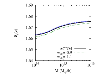
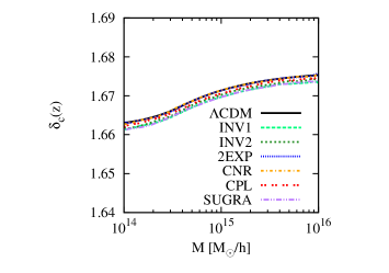
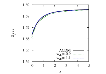
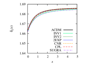
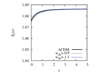
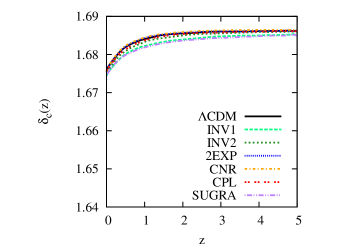
In Figure 1 we present the evolution of the linear extrapolated density parameter with (top panels) and without (bottom panels) the inclusion of the tidal shear, taking as reference model the CDM model (black solid line). Left (right) panels show models with a constant (dynamical) equation of state. In the caption we describe the different colours and line-styles of the models analysed in this work.
As already described in Reischke et al. (2016b) we restrict our treatment to masses above as smaller masses would lead to high values of as the cut-off of the power spectrum would be at higher . In this regime the treatment of the Zel’dovich approximation used to calculate the shear would break down and higher order effects which cannot be related to properties of the statistics of the underlying density field in a clear way need to be taken into account. Nonetheless the expected trend for smaller masses is an increase of the importance of tidal fields as the local fluctuations of the smoothed density field become larger.
As it appears clear from the top and middle rows of Figure 1 after a direct comparison with the corresponding panels in Fig. 7 of Reischke et al. (2016b), clustering dark energy models with the inclusion of the tidal shear resemble more closely the CDM model at all redshifts and at all mass scales with respect to the corresponding smooth models. This feature has been already observed in Batista & Pace (2013) for early dark energy models and we refer the reader to this work for a detailed explanation.
As expected, by construction, tidal shear has a bigger influence on small mass scales (). The linear extrapolated linear overdensity increases from () to (). In the high mass regime we notice a flattening of the curve, as in Reischke et al. (2016b), due to the fact that for these masses the effect of the tidal shear is completely negligible.
Note once again how differences between the CDM model and the dark energy models are minimal. By fixing the mass at , where we expect the biggest effect, we can also study the time evolution of with respect to the redshift . As explained in Reischke et al. (2016b) and in Sect. 3, the tidal shear is a function of both mass and time, with bigger effects at small redshifts, as it also happens for the parameter (defined via ) in Pace et al. (2014b). At high redshifts all the models recover very well an EdS universe since the effect of the tidal shear is negligible. At small redshifts all the models present slightly smaller values with respect to the case when the tidal shear is not included.
These results have the same qualitative behaviour of Pace et al. (2014b): bigger effect at small masses and redshifts and negligible effect at high masses and redshifts. Here nevertheless the effect is much smaller and is lower than for the standard spherical collapse model while the opposite takes place when the contribution of the angular momentum is included.
In general, we notice that the clustering of dark energy has negligible effects on the tidal shear as the equation of state had for the smooth case. This is due to the fact that tidal shear effects are important only at late times but theoretically tidal shear is evaluated at early times and as shown in Reischke et al. (2016b) this gives a per mill deviation from the standard spherical collapse model. In addition, at early times, all the models are approximately the same (dark energy perturbations and energy density are completely negligible with respect to the dark matter component) therefore the shear term is identical for all the models, as we verified numerically. This implies that the non-linear term due to shear is only a very small correction to the dynamical equations describing the spherical evolution.
The case presented and discussed here assumes that both dark matter and dark energy are affected in the same way by the tidal shear. We also studied a more general case where the tidal shear only affects the equations of motion of the dark matter component but not those of dark energy. Due to the above considerations, we could expect analogous results to before, as a direct inspection confirmed. Results are not only in qualitative, but also in quantitative agreement to what already discussed. The reason is due to that fact that linearised equations at early times are identical in both cases (by definition) and that the tidal shear is a very small contribution at such high redshifts. We will therefore not distinguish the two cases any more in the following. We also remark that the lack of differences between the two hypotheses was also found in Pace et al. (2014b).
5 Mass function and number counts
Within the framework of the Press & Schechter (Press & Schechter, 1974) and of the Sheth & Tormen (Sheth et al., 2001; Sheth & Tormen, 2002) formalism, knowing the time evolution of the growth factor (which describes the linear evolution of structures) and of the linear overdensity parameter , it is possible to evaluate the abundance of halos. A further parameter that needs to be specified is the normalization of the linear matter power spectrum . A theoretical derivation for the expression of the mass function within the theory of Gaussian random fields can be found in Press & Schechter (1974) and subsequently within the formalism of the excursion set (Bond et al., 1991). Due to its problems at both the low and high mass tail of the mass function, we decided to use the functional form provided in Sheth & Tormen (1999); Sheth et al. (2001); Sheth & Tormen (2002). Despite the fact that this improved formulation based on the ellipsoidal collapse model fits better the simulations at , it still has problems at high redshifts, where it significantly overestimates the number density of halos (Klypin et al., 2011). Limiting ourselves to low redshifts, we will use the Sheth & Tormen mass function formulation. We will also assume that this formulation can be safely extended to clustering dark energy models (but see also Del Popolo & Gambera, 1999; Del Popolo, 2006).
Before discussing in detail our finding, there is a further point we would like to clarify. The mass function and quantities derived, such has the number of halos above a given mass or in a range of redshifts, depend on the mass, but for clustering dark energy models there is an ambiguity in the definition of the mass to be used. When dark energy is smooth, the halo mass , assuming spherically symmetry and a top-hat profile as usually done within the formalism of the spherical collapse model, is , where is the halo virial radius and , where is the background matter density and the overdensity. When dark energy can cluster instead, in principle the mass of the halo should be influenced by the dark energy perturbations and these should be taken into account. Since different authors define this correction in different ways (Creminelli et al., 2010; Batista & Pace, 2013) and the contribution is nevertheless small (Basse et al., 2012) and here we are interested to the interplay of the tidal shear and the effective sound speed , we will not discuss this point further in our analysis.
Finally, a careful reader may wonder whether it is acceptable to use the Sheth & Tormen mass function also for clustering dark energy models. To our best knowledge, we think this is a good assumption for several reasons: to-date, only Press & Schechter (1974), Sheth et al. (2001) and Del Popolo (2006) proposed theoretically motivated formulations for the mass function, while all other analytic expressions (see Murray et al., 2013b, a, for a recent review) are fitting formulae to N-body simulations. Moreover, with the exception of Bhattacharya et al. (2011), all the others mass functions described in literature are tested again CDM cosmologies only. It would therefore be hard to know whether the fitted parameters would be changed in dark energy or clustering dark energy models. In addition, so far, there are no simulations allowing to study clustering dark energy in the fluid formalism and since all of the proposed mass functions agree reasonably well at and differ, due to a low number of objects, only at high mass, we conclude that the use of the mass function proposed in Sheth et al. (2001) is legit.
In the mass function formalism here adopted, the main theoretical quantity entering into the expression for the mass function is , where was discussed in the previous section and represents the evolution in time of the mass variance of the linear matter power spectrum. This quantity evolves proportionally to the linear growth factor, which is affected by cosmology only but not by the tidal shear. Differently from the standard spherical collapse model, now is also a function of mass and therefore we can expect a different shape of the mass function. This was also noticed and discussed in detail by Reischke et al. (2016b). In addition we recall that the tidal shear evolves differently from the linear growth factor, therefore the time evolution of will be affected as well and also this will have consequences on the overall mass function.
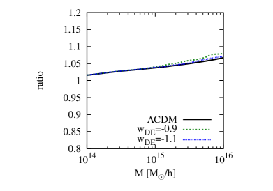
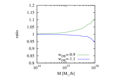
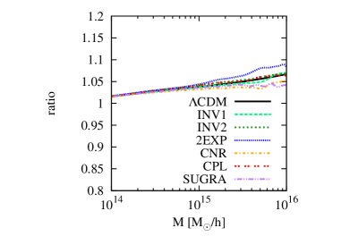
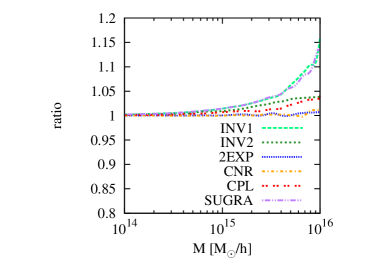
In figure 2 we show the cumulative comoving number density of objects above a given mass at ; in this way our analysis will not be affected by volume effects. In addition, we will also assume that all models have the same normalization of the matter power spectrum. Since from the above analysis it is clear that differences will be small, we prefer not to hide them behind normalization effects. For a better understanding of our findings we show the ratio between the dark energy and the CDM model. Left panels show the ratio between the models with and without tidal shear contribution while right panels show the ratio between the dark energy and the CDM model with tidal shear field.
The cumulative number density of objects above a given mass is defined as
| (22) |
where is the mass function evaluated at redshift . The minimum mass used is .
As a direct consequence of the analysis on the spherical collapse model, differences on the comoving number density are small. Smallest effects take place at low masses () and differences increase towards higher masses. At the highest mass probed here, differences are of the order of 10%, in perfect analogy with the case of smooth dark energy. Differences between the dark energy models and the reference CDM model are very small and noticeable mainly at high masses. This is in agreement with the fact that clustering dark energy models are more similar to the CDM model with respect to a smooth model. Differences are at most 3% for the 2EXP model. The top right panel shows models with a constant equation of state and we notice that both the quintessence and phantom models have a very similar behaviour, with the latter in particular very close to the CDM model. In the bottom right panel we show the same quantity, but for dynamical dark energy models. Once again the models behave very similarly to each other. Major effects take place for the 2EXP model while other models, such as the CPL and the INV1 and INV2 are practically indistinguishable from the CDM model.
Having established the relative effect of the tidal shear for each model, we now want to study the ratio between the dark energy models and the CDM one, when the tidal shear field is included for both. Results are in perfect qualitative agreement with what found in Reischke et al. (2016b) for smooth dark energy models. Starting with models with constant equation of state, quintessence (phantom) models predict more (less) objects with respect to the CDM model. Differences take place only at high masses and they are of the order of 10% (5%) for quintessence (phantom) models. These differences are very similar to the equivalent smooth models, differing by only 2-3%.
Qualitatively similar to the smooth scenario are also the dynamical dark energy models. Once again, these models, being in the quintessence regime, predict more objects than the CDM model and the relative number of objects grow with mass. Also for this set of models results are in qualitative agreement with the smooth scenario, albeit quantitative differences with respect to the CDM model are more limited. This is, once again, due to the fact that differences coming from are more limited. Models with higher differences are the INV1 and SUGRA, while the CNR and the 2EXP basically predict the same number of objects of the CDM model. Other models (INV2 and CPL) show intermediate values.
In Reischke et al. (2016b), the authors discuss the effect of tidal shear on the differential mass function and showed that its contribution is not enough to make the Press & Schechter mass function closer to the Sheth & Tormen one. Since also for clustering dark energy effects due to the inclusion of the tidal shear are small, we verified that a similar behaviour holds.
The effective sound speed of dark energy perturbations can affect several observational probes, such as the growth of matter perturbations, redshift space distortions and the shape of the dark matter power spectrum. These quantities will affect the weak lensing and the galaxy power spectrum which will be measured to a high level of accuracy by future surveys as Euclid (Amendola & et al., 2016). The observational probes mentioned will depend on the quantity which describes deviations from the standard Poisson equation: when dark energy is smooth (clustering), (). Assuming a null anisotropic stress, perturbations are fully described by which can be parametrised as (assuming a constant equation of state, Sapone & Kunz, 2009)
| (23) |
where is the matter density parameter today and . This expression is valid for both super- and sub-horizon scales. On scales inside the sound horizon, is sensitive to when dark energy is far from being smooth, i.e. . In other words, if dark energy is given by a minimally coupled scalar field, then its perturbations will be so small that we can neglect them.
Thanks to exquisite measurements in the weak and strong lensing regime, Euclid will be able to measure the halo mass function down to and therefore cover the mass regime studied in this work. Unfortunately, at these small scales it is necessary also to take into account effects from baryon physics and to understand the bias between the luminous and the dark matter component. Since these uncertainties can easily overcome the effect of tidal shear on the mass function, it might difficult to probe its effect. Also take into account that as shown in Reischke et al. (2016b), the error on cosmological parameters when not taking into account the tidal shear can be up to 1%. Since bigger effects will take place if , but at the same time the models will be closer to a CDM model than the corresponding smooth counterpart, it is necessary a combination of probes to disentangle the opposing physical effects.
6 Conclusions
By using the Zel’dovich approximation to sample the external tidal shear, we extend the work by Reischke et al. (2016b) to clustering dark energy models. In our formalism it is not possible to include the effects of rotation and therefore a direct comparison with Pace et al. (2014b) is not possible, since there the main contribution is given by the rotational term. Here we limit ourselves to a qualitative comparison.
As for the case of smooth dark energy, tidal shear effects are more relevant for small masses and for lower redshifts since with the growth of structures the curvature of the potential increases.
With respect to the standard spherical case and in analogy to the smooth dark energy model, tidal shear supports the collapse. Its effect on the spherical collapse parameter is of the order of few percent for the CDM model and for the clustering dark energy models analysed in this work. We notice that also when the tidal shear is included, clustering dark energy models resemble the CDM model more closely than a smooth dark energy model, as already explained for the standard spherical collapse model by Batista & Pace (2013).
Tidal shear affects the cumulative comoving number density of halos by few percent and major differences (of the order of 10%) arise at high masses. Similar effects, both at a qualitative and at a quantitative level, appear when comparing dark energy models with the CDM model. Comparing our results with Reischke et al. (2016b), we show that the clustering of dark energy is largely unaffected by tidal shear and results agree quantitatively with the smooth case. In Pace et al. (2014b), extending the work of Del Popolo et al. (2013a), the effect of shear and rotation was studied in clustering dark energy models. A direct comparison can not be performed since in these previous works the dominant term is the rotation one, therefore we can only discuss analogies and differences at a qualitative level. Both approaches lead to a mass-dependent term, the collapse is favoured and effects are at the percent level, differently from the aforementioned works. The effects of the additional rotation term will be included in a following work.
Several probes can be used to measure the effective sound speed of dark energy perturbations , but these are sensitive to it only if . Weak and strong lensing will be used to constrain the halo mass function and, as shown, effects will be appreciable in the case of fully clustering dark energy. On the other side, the linear extrapolated overdensity will be closer to the CDM model with respect to the smooth counterpart model, making therefore more difficult to measure the combined effects.
Acknowledgements
The authors thank an anonymous referee whose comments helped to improved the scientific content of this work. FP acknowledges support from a post-doctoral STFC fellowship and thanks Inga Cebotaru for carefully reading the manuscript and improve the style. RR acknowledges funding by the graduate college Astrophysics of cosmological probes of gravity by Landesgraduiertenakademie Baden-Württemberg.
References
- Abramo et al. (2007) Abramo L. R., Batista R. C., Liberato L., Rosenfeld R., 2007, Journal of Cosmology and Astro-Particle Physics, 11, 12
- Abramo et al. (2009a) Abramo L. R., Batista R. C., Rosenfeld R., 2009a, Journal of Cosmology and Astro-Particle Physics, 7, 40
- Abramo et al. (2009b) Abramo L. R., Batista R. C., Liberato L., Rosenfeld R., 2009b, Phys. Rev. D, 79, 023516
- Amendola & et al. (2016) Amendola L., et al. 2016, preprint, (arXiv:1606.00180)
- Amendola et al. (2013) Amendola L., et al., 2013, Living Reviews in Relativity, 16, 6
- Angrick & Bartelmann (2009) Angrick C., Bartelmann M., 2009, A&A, 494, 461
- Angrick & Bartelmann (2010) Angrick C., Bartelmann M., 2010, A&A, 518, A38
- Angrick et al. (2015) Angrick C., Pace F., Bartelmann M., Roncarelli M., 2015, MNRAS, 454, 1687
- Anselmi et al. (2011) Anselmi S., Ballesteros G., Pietroni M., 2011, J. Cosmology Astropart. Phys., 11, 014
- Avila-Reese et al. (1998) Avila-Reese V., Firmani C., Hernández X., 1998, ApJ, 505, 37
- Barboza & Alcaniz (2008) Barboza E. M., Alcaniz J. S., 2008, Physics Letters B, 666, 415
- Barreiro et al. (2000) Barreiro T., Copeland E. J., Nunes N. J., 2000, Phys. Rev. D, 61, 127301
- Basilakos (2009) Basilakos S., 2009, MNRAS, 395, 2347
- Basilakos et al. (2010) Basilakos S., Plionis M., Solà J., 2010, Phys. Rev. D, 82, 083512
- Basse et al. (2011) Basse T., Eggers Bjælde O., Wong Y. Y. Y., 2011, J. Cosmology Astropart. Phys., 10, 38
- Basse et al. (2012) Basse T., Eggers Bjaelde O., Hannestad S., Wong Y. Y. Y., 2012, preprint, (arXiv:1205.0548)
- Batista & Pace (2013) Batista R. C., Pace F., 2013, J. Cosmology Astropart. Phys., 6, 44
- Battye & Pace (2016) Battye R. A., Pace F., 2016, Phys. Rev. D, 94, 063513
- Bertschinger (1985) Bertschinger E., 1985, ApJS, 58, 39
- Bhattacharya et al. (2011) Bhattacharya S., Heitmann K., White M., Lukić Z., Wagner C., Habib S., 2011, ApJ, 732, 122
- Bond et al. (1991) Bond J. R., Cole S., Efstathiou G., Kaiser N., 1991, ApJ, 379, 440
- Bull et al. (2015) Bull P., Camera S., Raccanelli A., Blake C., Ferreira P., Santos M., Schwarz D. J., 2015, Proceedings of Advancing Astrophysics with the Square Kilometre Array (AASKA14),
- Camera et al. (2015) Camera S., et al., 2015, Proceedings of Advancing Astrophysics with the Square Kilometre Array (AASKA14),
- Chevallier & Polarski (2001) Chevallier M., Polarski D., 2001, International Journal of Modern Physics D, 10, 213
- Cole et al. (2005) Cole S., et al., 2005, MNRAS, 362, 505
- Copeland et al. (2000) Copeland E. J., Nunes N. J., Rosati F., 2000, Phys. Rev. D, 62, 123503
- Copeland et al. (2006) Copeland E. J., Sami M., Tsujikawa S., 2006, International Journal of Modern Physics D, 15, 1753
- Corasaniti (2004) Corasaniti P. S., 2004, PhD thesis, University of Sussex, http://de.arxiv.org/pdf/astro-ph/0401517
- Corasaniti & Copeland (2003) Corasaniti P. S., Copeland E. J., 2003, Phys. Rev. D, 67, 063521
- Creminelli et al. (2010) Creminelli P., D’Amico G., Noreña J., Senatore L., Vernizzi F., 2010, J. Cosmology Astropart. Phys., 3, 27
- Del Popolo (2002) Del Popolo A., 2002, A&A, 387, 759
- Del Popolo (2006) Del Popolo A., 2006, A&A, 448, 439
- Del Popolo & Gambera (1999) Del Popolo A., Gambera M., 1999, A&A, 344, 17
- Del Popolo et al. (2013a) Del Popolo A., Pace F., Lima J. A. S., 2013a, International Journal of Modern Physics D, 22, 50038
- Del Popolo et al. (2013b) Del Popolo A., Pace F., Maydanyuk S. P., Lima J. A. S., Jesus J. F., 2013b, Phys. Rev. D, 87, 043527
- Del Popolo et al. (2013c) Del Popolo A., Pace F., Lima J. A. S., 2013c, MNRAS, 430, 628
- Diego & Majumdar (2004) Diego J. M., Majumdar S., 2004, MNRAS, 352, 993
- Fang & Haiman (2007) Fang W., Haiman Z., 2007, Phys. Rev. D, 75, 043010
- Ferreira & Joyce (1998) Ferreira P. G., Joyce M., 1998, Phys. Rev. D, 58, 023503
- Fillmore & Goldreich (1984) Fillmore J. A., Goldreich P., 1984, ApJ, 281, 1
- Fosalba & Gaztan̈aga (1998) Fosalba P., Gaztan̈aga E., 1998, MNRAS, 301, 503
- Gleyzes et al. (2013) Gleyzes J., Langlois D., Piazza F., Vernizzi F., 2013, J. Cosmology Astropart. Phys., 8, 025
- Gleyzes et al. (2014) Gleyzes J., Langlois D., Vernizzi F., 2014, International Journal of Modern Physics D, 23, 1443010
- Gunn & Gott (1972) Gunn J. E., Gott III J. R., 1972, ApJ, 176, 1
- Haiman et al. (2001) Haiman Z., Mohr J. J., Holder G. P., 2001, ApJ, 553, 545
- Hannestad & Mörtsell (2004) Hannestad S., Mörtsell E., 2004, J. Cosmology Astropart. Phys., 9, 001
- Heavens & Sheth (1999) Heavens A. F., Sheth R. K., 1999, MNRAS, 310, 1062
- Holder et al. (2001) Holder G., Haiman Z., Mohr J. J., 2001, ApJ, 560, L111
- Jassal et al. (2005) Jassal H. K., Bagla J. S., Padmanabhan T., 2005, Phys. Rev. D, 72, 103503
- Jennings et al. (2010) Jennings E., Baugh C. M., Angulo R. E., Pascoli S., 2010, MNRAS, 401, 2181
- Klypin et al. (2011) Klypin A. A., Trujillo-Gomez S., Primack J., 2011, ApJ, 740, 102
- LSST Dark Energy Science Collaboration (2012) LSST Dark Energy Science Collaboration 2012, preprint, (arXiv:1211.0310)
- Laureijs et al. (2011) Laureijs R., et al., 2011, ArXiv e-prints, 1110.3193,
- Linder (2003) Linder E. V., 2003, Physical Review Letters, 90, 091301
- LoVerde (2014) LoVerde M., 2014, Phys. Rev. D, 90, 083518
- Majumdar (2004) Majumdar S., 2004, Pramana, 63, 871
- Majumdar & Mohr (2003) Majumdar S., Mohr J. J., 2003, ApJ, 585, 603
- Maturi et al. (2010) Maturi M., Angrick C., Pace F., Bartelmann M., 2010, A&A, 519, A23
- Maturi et al. (2011) Maturi M., Fedeli C., Moscardini L., 2011, MNRAS, 416, 2527
- Mota & van de Bruck (2004) Mota D. F., van de Bruck C., 2004, A&A, 421, 71
- Murray et al. (2013a) Murray S. G., Power C., Robotham A. S. G., 2013a, Astronomy and Computing, 3, 23
- Murray et al. (2013b) Murray S. G., Power C., Robotham A. S. G., 2013b, MNRAS, 434, L61
- Nazari-Pooya et al. (2016) Nazari-Pooya N., Malekjani M., Pace F., Jassur D. M.-Z., 2016, MNRAS, 458, 3795
- Nunes & Mota (2006) Nunes N. J., Mota D. F., 2006, MNRAS, 368, 751
- Ohta et al. (2003) Ohta Y., Kayo I., Taruya A., 2003, ApJ, 589, 1
- Ohta et al. (2004) Ohta Y., Kayo I., Taruya A., 2004, ApJ, 608, 647
- Pace et al. (2010) Pace F., Waizmann J.-C., Bartelmann M., 2010, MNRAS, 406, 1865
- Pace et al. (2012) Pace F., Fedeli C., Moscardini L., Bartelmann M., 2012, MNRAS, 422, 1186
- Pace et al. (2014a) Pace F., Moscardini L., Crittenden R., Bartelmann M., Pettorino V., 2014a, MNRAS, 437, 547
- Pace et al. (2014b) Pace F., Batista R. C., Del Popolo A., 2014b, MNRAS, 445, 648
- Padmanabhan (1993) Padmanabhan T., 1993, Structure Formation in the Universe
- Padmanabhan (1996) Padmanabhan T., 1996, Cosmology and Astrophysics through Problems
- Perlmutter et al. (1999) Perlmutter S., Aldering G., Goldhaber G., et al. 1999, ApJ, 517, 565
- Planck Collaboration XIII (2016) Planck Collaboration XIII 2016, A&A, 594, A13
- Planck Collaboration XIV (2016) Planck Collaboration XIV 2016, A&A, 594, A14
- Press & Schechter (1974) Press W. H., Schechter P., 1974, ApJ, 187, 425
- Regos & Szalay (1995) Regos E., Szalay A. S., 1995, MNRAS, 272, 447
- Reischke et al. (2016a) Reischke R., Maturi M., Bartelmann M., 2016a, MNRAS, 456, 641
- Reischke et al. (2016b) Reischke R., Pace F., Meyer S., Schäfer B. M., 2016b, MNRAS, 463, 429
- Riess et al. (1998) Riess A. G., Filippenko A. V., Challis P., et al. 1998, AJ, 116, 1009
- Ryden & Gunn (1987) Ryden B. S., Gunn J. E., 1987, ApJ, 318, 15
- Sánchez et al. (2009) Sánchez A. G., Crocce M., Cabré A., Baugh C. M., Gaztañaga E., 2009, MNRAS, 400, 1643
- Santos et al. (2015) Santos M. G., et al., 2015, Proceedings of Advancing Astrophysics with the Square Kilometre Array (AASKA14),
- Sapone & Kunz (2009) Sapone D., Kunz M., 2009, Phys. Rev. D, 80, 083519
- Schäfer & Merkel (2012) Schäfer B. M., Merkel P. M., 2012, MNRAS, 421, 2751
- Sheth & Tormen (1999) Sheth R. K., Tormen G., 1999, MNRAS, 308, 119
- Sheth & Tormen (2002) Sheth R. K., Tormen G., 2002, MNRAS, 329, 61
- Sheth et al. (2001) Sheth R. K., Mo H. J., Tormen G., 2001, MNRAS, 323, 1
- Szydłowski et al. (2006) Szydłowski M., Kurek A., Krawiec A., 2006, Physics Letters B, 642, 171
- Tarrant et al. (2012) Tarrant E. R. M., van de Bruck C., Copeland E. J., Green A. M., 2012, Phys. Rev. D, 85, 023503
- Tsujikawa (2010) Tsujikawa S., 2010, ArXiv e-prints, 1004.1493,
- Weller et al. (2002) Weller J., Battye R. A., Kneissl R., 2002, Physical Review Letters, 88, 231301
- Wintergerst & Pettorino (2010) Wintergerst N., Pettorino V., 2010, Phys. Rev. D, 82, 103516
- Zel’Dovich (1970) Zel’Dovich Y. B., 1970, A&A, 5, 84