Physical conditions for Jupiter-like dynamo models

Abstract

The Juno mission will measure Jupiter’s magnetic field with unprecedented precision and provide a wealth of additional data that will allow us to constrain the planet’s interior structure and dynamics. Here we analyse $66$ different numerical simulations in order to explore the sensitivity of the dynamo-generated magnetic field to the planets interior properties. Jupiter field models based on pre-Juno data and up-to-date interior models based on ab initio simulations serve as benchmarks. Our results suggest that Jupiter-like magnetic fields can be found for a number of different models. These complement the steep density gradients in the outer part of the simulated shell with an electrical conductivity profile that mimics the low conductivity in the molecular hydrogen layer and thus renders the dynamo action in this region largely unimportant. We find that whether we assume an ideal gas or use the more realistic interior model based on ab initio simulations makes no difference. However, two other factors are important. A low Rayleigh number leads to a too strong axial dipole contribution while the axial dipole dominance is lost altogether when the convective driving is too strong. The required intermediate range that yields Jupiter-like magnetic fields depends on the other system properties. The second important factor is the convective magnetic Reynolds number radial profile $Rm_{c}(r)$, basically a product of the non-axisymmetric flow velocity and electrical conductivity. We find that the depth where $Rm_{c}$ exceeds about $50$ is a good proxy for the top of the dynamo region. When the dynamo region sits too deep, the axial dipole is once more too dominant due to geometric reasons. Extrapolating our results to Jupiter and the result suggests that the Jovian dynamo extends to $95$% of the planetary radius.

The zonal flow system in our simulations is dominated by an equatorial jet which remains largely confined to the molecular layer. Where the jet reaches down to higher electrical conductivities, however, it gives rise to a secondary $\alpha\Omega$ dynamo that modifies the dipole-dominated field produced deeper in the planet. This secondary dynamo can lead to strong magnetic field patches at lower latitudes that seem compatible with the pre-Juno field models.

1 Introduction

The interior dynamics of Jupiter has been the topic of an increasing number of studies over the last ten years (Heimpel et al., 2005; Lian and Showman, 2008; Stanley and Glatzmaier, 2010; Kaspi et al., 2009; Heimpel and Gómez-Pérez, 2011; Gastine and Wicht, 2012; Duarte et al., 2013; Gastine et al., 2014b; Jones, 2014; Heimpel et al., 2016). The growing interest is at least partially motivated by two Jovian space missions. NASA’s Juno spacecraft arrived in summer 2016 and started to measure the planet’s magnetic field with unprecedented precision. It will also provide important information on the inner structure and dynamics, for example via gravity data. ESA’s Jupiter system mission Juice is scheduled to be launched in 2022.

Recent models for Jupiter’s interior structure combine pre-Juno gravity and planetary figure measurements with refined equations of state that are based on ab initio calculations (French et al., 2012; Nettelmann et al., 2012). These models assume a small rocky core of uncertain size and a two layer Hydrogen and Helium envelope where the inner layer contains more heavy elements than the outer. When pressures are high enough at about $80$ to $90$% of Jupiter’s radius, hydrogen undergoes a phase transition from the molecular to a metallic state (e.g. Chabrier et al., 1992; Fortney and Nettelmann, 2010; Nettelmann et al., 2012). Since this transition lies beyond the triple point (French et al., 2012) there is no sharp change in the physical properties. Using advanced ab initio calculations, French et al. (2012) shows that the electrical conductivity, a particularly important property for the dynamo process, rises steeply with depth at a super-exponential rate in the molecular layer and then more smoothly transitions into the metallic region where the gradient becomes much shallower (see Fig. 2).

Magnetic field models in the pre-Juno era rely on a few flybys and sometimes auroral information to constrain spherical harmonic surface field contributions up to degree $\ell\!=\!4$ (Connerney et al., 1998; Grodent et al., 2008; Hess et al., 2011) or $\ell\!=\!7$ at best (Ridley, 2012; Ridley and Holme, 2016). Due to its dedicated polar orbit, Juno is expected to constrain models up to $\ell\!=\!15$ or higher. This exceeds the resolution available for Earth where the crustal field shields harmonics beyond $\ell\simeq 14$.

While the magnetic field offers indirect clues for the deeper processes the surface dynamics can be inferred more directly, for example by tracking cloud features. The surface winds are dominated by a system of zonal jets where a fast prograde equatorial jet is flanked by several additional jets of alternating retrograde and prograde direction. At least the equatorial jet could be a geostrophic structure that reaches through the planets and is maintained by Reynolds stresses, a statistical correlation between smaller-scale convective flow components (Christensen, 2001; Heimpel et al., 2005; Gastine and Wicht, 2012; Gastine et al., 2012). This is less clear for the flanking jets which may be much shallower thermal-wind driven structures (Kaspi et al., 2009). Constraining the depth of Jupiter’s jet system is one of the main objectives of the Juno mission.

Though the ab initio simulations may not support a clear separation, traditional simulations of Jupiter’s internal dynamics concentrated on either describing the deeper dynamo thought to operate in the metallic hydrogen layer or on the jet dynamics in the molecular envelope. While the latter are very successful in describing the observed zonal jet structure (Heimpel et al., 2005; Gastine et al., 2014a; Heimpel et al., 2016) the dynamo simulation have proven to be more problematic. Since Jupiter’s magnetic field has a very Earth-like configuration is it tempting to assume that numerical geodynamo simulations capture the dynamics of the metallic layer. However, geodynamo models typically neglect compressibility and assume a constant adiabatic temperature profile in the so-called Boussinesq approximation. Moreover, the electrical conductivity is constant and rigid flow boundary conditions are often used that significantly inhibit zonal winds (Olson et al., 1999; Christensen and Wicht, 2007). These simulations show that dipolar and thus Earth-like or Jupiter-like magnetic fields can only be expected when the system is not driven too strongly, i.e. the Rayleigh number remains in a range where inertial effects are small (Christensen and Aubert, 2006).

More recent simulations have shown that it becomes increasingly complicated to maintain dipole-dominated fields when modifying the models to better represent gas planets. Using stress free rather than rigid flow boundary conditions allows strong Reynolds-stress driven zonal winds to develop, which are always highly geostrophic and thus reach through the whole gaseous envelope. The competition between these winds and strong dipolar fields plays an important role in determining whether the magnetic field becomes axial dipole-dominated or multipolar, i.e. more complex without a dominant axial dipole contribution (Grote and Busse, 2000; Busse and Simitev, 2006; Simitev and Busse, 2009; Sasaki et al., 2011; Schrinner et al., 2012; Gastine et al., 2012). Zonal flows tend to promote weaker multipolar fields while strong dipole fields can suppress the zonal flows via Lorentz forces. Dipole-dominated dynamos thus require a certain balance between flow vigour and dipole field amplitude.

A consequence of this competition is the bistability found at not too large Rayleigh numbers where dipole and multipole solutions coexist at identical parameters (Gastine et al., 2012). The multipolar branch is reached when starting a simulation with a weak field and is characterized by stronger zonal flows. Establishing a solution on the dipolar branch, on the other hand, requires to start with a strong dipole that sufficiently suppresses the zonal flows (e.g. Schrinner et al., 2012). When the Rayleigh number is increased beyond a certain point only the multipolar branch remains. However, the simple rule that describes this transition for Earth-like dynamos in terms of the relative importance of inertia (Christensen and Aubert, 2006) does mostly not apply in gas giants (Duarte et al., 2013).

Including Jupiter-like density profiles in the so-called anelastic approximation (Gilman and Glatzmaier, 1981; Glatzmaier, 1984; Braginsky and Roberts, 1995; Lantz and Fan, 1999) yields further difficulties. The density stratification leads to convective flows where the amplitude increases with radius while the length scale decreases. The zonal flow system changes less dramatically but nevertheless significantly: the equatorial jet becomes somewhat more confined and increases in amplitude while the mid to higher latitude jets slow down (Gastine and Wicht, 2012).

More successful are integrated models that include the molecular envelope and more specifically the steep decrease in electrical conductivity (Gastine et al., 2014b; Jones, 2014). This allows the strong equatorial jet to remain mostly constrained to the weakly conducting outer envelope and thus participate little in the primary dynamo action (Gastine et al., 2012, 2014b). The dipole field actually contributes to establishing itself by pushing the equatorial jet to the weakly conducting shell and by braking the remaining high to mid latitude zonal flows via Lorentz forces (Duarte et al., 2013). When the weakly conducting shell is too thick, however, the region where the Lorentz force can counteract zonal wind production via Reynolds stresses becomes too restricted and the dynamo ends up producing a multipolar field.

Another effect that can help establishing a dipole-dominated field is an increased magnetic Prandtl number $Pm\!=\!\nu/\lambda$ where $\nu$ is the kinematic viscosity and $\lambda\!=\!1/(\sigma\mu_{0})$ the magnetic diffusivity (Duarte et al., 2013; Schrinner et al., 2014; Jones, 2014; Raynaud et al., 2015). Increasing $Pm$ is equivalent to increasing the electrical conductivity $\sigma$ which leads to a more efficient dynamo and likely also stronger Lorentz forces that can more easily balance zonal flows. Several authors also report that either decreasing or increasing the Prandtl number $Pr\!=\!\nu/\kappa$ (ratio of kinematic viscosity $\nu$ to thermal diffusivity $\kappa$), from a typical value of $Pr\!=\!1$ used in many simulations to $0.1$ or $10$, respectively, may also help (Jones, 2014; Yadav et al., 2015b, a). Jones (2014) argues that at low $Pr$ the convection is more evenly distributed throughout the shell which leads to a less dominant equatorial jet and stronger dipole field generated at depth, while higher $Pr$ means reduced inertia (Yadav et al., 2015b). The effect is potentially important for Jupiter where $Pr$ may be as low as $10^{-2}$ at depth (French et al., 2012).

The Ekman number $E$ is another parameter that can influence the magnetic field configuration. $E$ is a measure for the ratio of viscous to Coriolis forces in the flow force balance. Because of the small viscosity and fast planetary rotation, Jupiter’s Ekman number is only about $10^{-18}$. For the simulations, however, a much higher viscosity is assumed to damp the small scale convection that cannot be resolved numerically and $E$ is typically of order $10^{-4}$ or $10^{-5}$. Boussinesq dynamo simulations suggest that a lower $E$ promotes dipolar fields because the stronger Coriolis forces help to organize large scale magnetic field generation (Christensen and Aubert, 2006; Wicht and Christensen, 2010). Since Heimpel and Gómez-Pérez (2011); Duarte et al. (2013) suggest that a lower $10^{-5}$ may also help to establish dipolar dynamos in anelastic simulations it seems important to further explore this issue.

Many authors drive convection in their Jupiter models from the bottom (Gastine et al., 2012; Duarte et al., 2013; Gastine et al., 2014b) as would be more appropriate for Earth. Heat enters the modelled spherical shell through the inner and leaves it through the outer boundary. However, internal heat sources seem more realistic for modelling the secular cooling that drives convection in Jupiter. Jones (2014) reports that internal heating makes it less likely to find a dipole-dominated dynamo.

In the most realistic simulation to date, Gastine et al. (2014b) reproduce many distinct features of the pre-Juno Jovian magnetic field. This includes the field strength, dipole dominance, dipole tilt, magnetic power spectrum and secular variation estimates (Connerney et al., 1998; Ridley and Holme, 2016). Their model, that we will refer to as G14 in the following, covers $99$% of the Jovian density profile suggested by French et al. (2012) and uses an electrical conductivity profile with a significant conductivity decrease in the molecular layer. Here we extend the G14 study by analysing a larger number of different model set-ups with respect to their capability of reproducing Jupiter’s magnetic field. Our data set includes $66$ simulations with different parameters, different density profiles, different electrical conductivity profiles, and different driving modes. The paper is organized as follows: after introducing the numerical model in Sec. 2 we analyse the simulation results in Sec. 3, and close with a discussion in Sec. 4.

2 Model

We adopt the anelastic formulation suggested by Gilman and Glatzmaier (1981), Braginsky and Roberts (1995) and Lantz and Fan (1999). This allows to consider background density and temperature variations but filters out sounds waves which would required a significantly smaller time step. MagIC actually solves for small variations around a background state which is assumed to be hydrostatic, adiabatic and non-magnetic. In the following, all quantities with a tilde characterize the dimensionless background state.

2.1 Background state

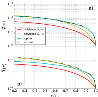
Figure 1: Density (a) and temperature (b) background profiles used in this work. The cyan line corresponds to our fit to the ab initio calculations by Nettelmann et al. (2012) for the innermost $99\%$ of Jupiter, represented by black dotted line (see also French et al., 2012). The overlap is nearly perfect for $\tilde{\rho}$ but the $\tilde{T}$ fit deviates at $r\!<\!0.85r_{o}$. The red and yellow lines show the polytropic background reference states of $N_{\rho}\!=\!4$ and $N_{\rho}\!=\!5$ respectively with polytropic index $n\!=\!2$. To ease the comparison, the density and temperature profiles from the ab initio calculation have been normalised by their values at $r\!=\!0.99\,R_{\jupiter}$.

Figure 1a shows the three different density background profiles considered here. Several of our models, corresponding to the cyan profiles in Fig. 1a,b, rely on the interior properties suggested by French et al. (2012). Starting point is the French et al. (2012) density $\tilde{\rho}(r)$ profile that is approximated by a polynomial of degree seven. Due to numerical limitations we can only simulate $99\%$ of Jupiter’s radius and have to ignore the outermost $1$% where the density gradient is the steepest. The density polynomial is then fitted with a power law $\tilde{T}\!=\!\textrm{const. }\tilde{\rho}^{1/n^{*}}$ (Fig. 1b). We find that an exponent $n^{*}\!=\!2.22$ yields the best fit. The pressure closely obeys a profile with polytropic index $n\!=\!1$ (Hubbard, 1975):

$$\tilde{p}\sim\tilde{\rho}^{(n+1)/n}\sim\tilde{\rho}^{2}\textrm{,}$$ (1)

where $p$ is pressure. The difference between the exponents $n$ and $n^{*}$ demonstrates that Jupiter’s interior strongly deviates from an ideal gas behavior where both would be identical ($n\!=\!n^{*}$). The product of thermal expansivity and gravity that appears in the buoyancy term of the Navier-Stokes equation, Eq. 4, is directly related to the background temperature profile via

$$\frac{1}{\tilde{T}}\frac{\mathrm{d}\tilde{T}}{\mathrm{d}r}=-Di\,\tilde{\alpha}\tilde{g}\;\;{\textrm{,}}$$ (2)

where $Di\!=\!\alpha_{o}g_{o}d/c_{p}$ is the dissipation number based on the outer boundary reference gravity $g_{o}$ and the reference thermal expansivity $\alpha_{o}$. Here $\tilde{\alpha}\!=\!\alpha/\alpha_{o}$ is the normalized thermal expansivity profile, $\tilde{g}\!=\!g/g_{o}$ the normalized gravity profile, $c_{p}$ is the heat capacity at constant pressure and $d\!=\!r_{o}-r_{i}$ is the difference between outer shell radius $r_{o}$ and inner shell radius $r_{i}$ that we use as length scale to non-dimensionalize the equations. Since this background model has first been adopted by G14 we refer to this background model as BG-G14  in the following.

The yellow and red profiles in Fig. 1 illustrate the two other background state models used here. For simplicity, we assume a temperature gradient proportional to radius, $\mathrm{d}\tilde{T}/\mathrm{d}r\!=\!-Di\,r/r_{o}$, and a polytrope-like density profile $\tilde{\rho}\!=\!\tilde{T}^{1/n}$ with a polytrope index $n\!=\!2$ halfway between $n\!=\!3/2$ for a mono-atomic and $n\!=\!5/2$ for a bi-atomic gas. For an ideal gas with $\alpha\!=\!1/\tilde{T}$ the temerature gradient would imply $g\!\sim\!r$ which is realistic for a homogeneous density but not the polytrope profile.

While not realistic for Jupiter these setups nevertheless serve to explore the sensitivity of our models to the background state. The absolute density contrast is controlled by $N_{\rho}\!=\!\ln\left[\tilde{\rho}(r_{i})/\tilde{\rho}(r_{o})\right]$, the number of density scale heights covered between the inner ($r_{i}$) and the outer ($r_{o}$) boundaries. We consider simulations with $N_{\rho}\!=\!4$ or $N_{\rho}\!=\!5$ that we refer to as ’polytrope’ models in the following. Figure 1a illustrates that the respective density profiles are more gradual than the BG-G14 counterpart where most of the density drop is concentrated at larger radii.

Ab initio simulations by (French et al., 2012) yield an electrical conductivity profile for the interior of Jupiter that is illustrated in Fig. 2). A super-exponential increase in the molecular layer until about $0.9R_{\jupiter}$ smoothly transitions into a much shallower gradient in the metallic layer. Since the super-exponential increase causes numerical difficulties, we use several simplified conductivity profiles with a constant interior conductivity branch that is matched to an exponentially decaying outer branch via a polynomial that assures a continuous first derivative (Gómez-Pérez et al., 2010):

$$\tilde{\sigma}(r)=\left\{\begin{array}[]{ll}1+(\tilde{\sigma}_{m}-1)\,\Bigg{(}\dfrac{r-r_{i}}{r_{m}-r_{i}}\Bigg{)}^{a}&r<r_{m}\\ \tilde{\sigma}_{m}\exp{}\left[a\,\frac{r-r_{m}}{r_{m}-r_{i}}\,\frac{\tilde{\sigma}_{m}-1}{\tilde{\sigma}_{m}}\right]&r\geq r_{m}\end{array}\right.\textrm{.}$$ (3)

The tilde once more signifies the non-dimensional background state where we have used the inner-boundary conductivity value as a reference value $\sigma_{i}$. Free parameters are the rate of the exponential decay $a$ and the radius $r_{m}$ and conductivity value $\sigma_{m}$ for the transition between both branches. For convenience we also define the relative transition radius in percentage: $\chi_{m}\!=\!r_{m}/r_{o}$. The non-dimensional magnetic diffusivity profile is given by $\tilde{\lambda}(r)=\lambda(r)/\lambda_{i}=\sigma_{i}/\sigma(r)=1/\tilde{\sigma}(r)$ where the tilde signifies the non-dimensional background state.

Figure 2 compares the electrical conductivity profiles mostly used in this study with the profile by French et al. (2012). A series of profiles with $\chi_{m}\!=\!0.8$, $\sigma_{m}\!=\!0.5$ and increasing decay rates from $a\!=\!9$ to $a\!=\!40$ serves to explore the potential influence of the decay rate. In the most extreme model with $a\!=\!40$ the conductivity decrease by seven orders of magnitude. G14 use $\chi_{m}\!=\!0.9$, $\sigma_{m}\!=\!0.2$, and $a\!=\!13$ which yields a profile (cyan) where the higher conductivity inner region reaches further out, the transition to the exponential decay is smoother, and the total decrease amounts to four orders of magnitude. That is also the profile adopted for most of our new simulations. An additional ’early decaying’ profile (yellow line in Fig. 2) tries to model the slower conductivity decrease predicted for the inner metallic layer with a linear decay rate.

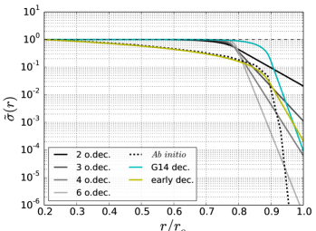
Figure 2: Radial profiles of normalized electrical conductivity, to illustrate the flexibility of Eq. 3. The black dotted line corresponds to the ab initio calculation from French et al. (2012). The grey-coloured profiles differ only in $a$ and represent profiles already used in Duarte et al. (2013) with $\sigma_{m}\!=\!0.5$, $r_{m}\!=\!80$, and $a\!=\!9$ (black, approximately 2 orders of magnitude decay), $a\!=\!17$ (dark grey, $\sim 3$ oom), $a\!=\!25$ (medium grey, $\sim 4$ oom) and $a\!=\!40$ (light grey, $\sim 6$ oom). The yellow line illustrates the ’earlier decaying’ profile that mimics the ab initio result in the metallic interior, using $a\!=\!1.0$, $\sigma_{m}\!=\!0.03$, $r_{m}\!=\!90$. The cyan line shows the profile with $a\!=\!13.0$, $\sigma_{m}\!=\!0.2$, $r_{m}\!=\!90$ mostly used by G14 and in most of our new simulations. All profiles have been normalized with the electrical conductivity at the inner boundary.

2.2 Anelastic equations

We solve for convection and magnetic field generation in a rotating spherical shell with outer radius $r_{o}$ and inner radius $r_{i}$. The set of anelastic equations that describes the evolution of the dimensionless velocity $\mathbf{u}$, magnetic field $\mathbf{B}$ and specific entropy $s$ are the Navier-Stokes equation, dynamo equation, energy equation and continuity equations:

$$\begin{split}E\,\bigg{(}\frac{\partial\mathbf{u}}{\partial t}+\mathbf{u}\cdot\nabla\mathbf{u}\bigg{)}=&-\nabla\frac{p}{\tilde{\rho}}-2\mathbf{e}_{z}\times\mathbf{u}-\frac{Ra\,E}{Pr\,Di}\frac{d\tilde{T}}{dr}s\,\mathbf{e}_{r}\\ &+\frac{1}{Pm_{i}\,\tilde{\rho}}(\nabla\times\mathbf{B})\times\mathbf{B}+\frac{E}{\tilde{\rho}}\nabla\cdot\textsf{S}\;\;{\textrm{,}}\end{split}$$ (4)

$$\frac{\partial\mathbf{B}}{\partial t}=\nabla\times(\mathbf{u}\times\mathbf{B})-\frac{1}{Pm_{i}}\nabla\times(\tilde{\lambda}\nabla\times\mathbf{B})\;\;{\textrm{,}}$$ (5)

$$\begin{split}\tilde{\rho}\,\tilde{T}\,\bigg{(}\frac{\partial s}{\partial t}+\mathbf{u}\cdot\nabla s\bigg{)}=&\frac{1}{Pr}\nabla\cdot(\tilde{\rho}\tilde{T}\nabla s)+\epsilon\tilde{\rho}\\ &+\frac{Pr\,Di}{Ra}\left[\textsf{S}^{2}+\frac{\tilde{\lambda}}{Pm_{i}^{2}\,E}(\nabla\times\mathbf{B})^{2}\right]\;\;{\textrm{,}}\end{split}$$ (6)

$$\nabla\cdot(\tilde{\rho}\mathbf{u})=0\;\;{\textrm{,}}$$ (7)

$$\nabla\cdot\mathbf{B}=0\;\;{\textrm{.}}$$ (8)

Here S is the traceless rate-of-strain tensor for an homogeneous kinematic viscosity,

$$\textsf{S}=2\tilde{\rho}\bigg{[}\textsf{e}_{ij}-\frac{1}{3}\delta_{ij}\nabla\cdot\mathbf{u}\bigg{]}\;\;\;\textrm{ and }\;\;\;\textsf{e}_{ij}=\frac{1}{2}\bigg{(}\frac{\partial u_{i}}{\partial x_{j}}+\frac{\partial u_{j}}{\partial x_{i}}\bigg{)}\;\;{\textrm{,}}$$ (9)

where $\delta_{ij}$ is the identity matrix. The terms inside the square brackets of Eq. 6 correspond to the viscous and ohmic heating contributions.

These equations have been non-dimensionalized using shell thickness $d\!=\!r_{o}-r_{i}$ as the length scale and the viscous diffusion time $\tau_{\nu}\!=\!d^{2}/{\nu}$ as a timescale. Temperature and density are non-dimensionalized by their values at the outer boundary, $T_{o}$ and $\rho_{o}$. We employ either constant entropy or constant entropy flux boundary conditions. In the former case, the imposed super-adiabatic contrast $\Delta s$ across the shell serves as the specific entropy scale $S$. In the latter case the outer boundary heat flux $q_{o}$ defines $S\!=\!q_{o}d\alpha_{o}/\rho_{o}\kappa$ where $\kappa$ is the constant thermal diffusivity. The magnetic field unit is $\sqrt{\Omega\mu_{0}\lambda_{i}\rho_{o}}$, where $\Omega$ is the system rotation rate.

In addition to the parameters that define the background state, Eqs. (4–8) are controlled by the Ekman number $E$, the Rayleigh number $Ra$, the Prandtl number $Pr$ and the magnetic Prandtl number at the inner boundary $Pm_{i}$:

$$E=\frac{\nu}{\Omega d^{2}}\textrm{,}$$ (10)

$$Ra=\frac{g_{o}d^{3}S}{c_{p}\nu\kappa}\textrm{,}$$ (11)

$$Pr=\frac{\nu}{\kappa}\textrm{,}$$ (12)

$$Pm_{i}=\frac{\nu}{\lambda_{i}}\textrm{.}$$ (13)

To characterize the mean magnetic Prandtl number we introduce the volume-averaged

$$Pm_{V}=\frac{Pm_{i}}{V}\int_{r_{i}}^{r_{o}}4\,\pi\,\tilde{\sigma}(r)\,r^{2}\,\mathrm{d}r\,\textrm{,}$$ (14)

where $V$ is the volume of the spherical shell.

We will measure the dimensionless rms amplitude of the flow by the Rossby number

$$Ro=E\,\left(\,\int\mathbf{u}\cdot\mathbf{u}\,dV\,\right)^{1/2}\textrm{ ,}$$ (15)

where $\mathbf{u}$ in this work is either only the azimuthal component of the flow velocity or the non-axisymmetric, $Ro_{zon}$ and $Ro_{c}$ respectively (see Tab. LABEL:TabRes). The analogous dimensionless rms magnetic field strength is given by the Lorentz number,

$$Lo=\left(\;\frac{E}{Pm_{i}}\frac{\int B^{2}\,dV}{\int\tilde{\rho}\,dV}\;\right)^{1/2}\textrm{ ,}$$ (16)

in the form introduced by Yadav et al. (2013b). The relative importance of the Lorentz force compared to the Coriolis force is typically quantified by the Elsasser number,

$$\Lambda=\int\frac{\mathbf{B}^{2}}{\tilde{\rho}\tilde{\lambda}}\,dV\textrm{ .}$$ (17)

Decisive for dynamo action is not the electrical conductivity or magnetic diffusivity but the magnetic Reynolds number $Rm\!=\!Ud/\lambda$, a combination with a typical flow velocity $U$. $Rm$ is a crude measure for the ratio of magnetic field production to Ohmic dissipation. We introduce a radial dependent convective magnetic Reynolds number

$$Rm_{c}(r)=\frac{U_{c}(r)d}{\lambda(r)}\;\;{\textrm{,}}$$ (18)

where $U_{c}(r)$ denotes the rms amplitude of non-axisymmetric flows at radius $r$. We will also refer to the volume-averaged value

$$Rm=\frac{3}{r_{o}^{3}-r_{i}^{3}}\bigintssss_{r_{i}}^{r_{o}}\!Rm_{c}(r)\,r^{2}\,\mathrm{d}r\textrm{.}$$ (19)

2.3 Numerical methods

The anelastic equations 4 to 6 are solved with the MHD code MagIC (Wicht, 2002; Gastine and Wicht, 2012). MagIC has been benchmarked (Jones et al., 2011) and is one of the fastest codes of its class (Matsui et al., 2016). Poloidal/toroidal decompositions,

$$\begin{split}\tilde{\rho}\vec{u}&=\vec{\nabla}\times\left(\vec{\nabla}\times W\vec{e_{r}}\right)+\vec{\nabla}\times Z\vec{e_{r}}\;\;{\textrm{,}}\\ \vec{B}&=\vec{\nabla}\times\left(\vec{\nabla}\times C\vec{e_{r}}\right)+\vec{\nabla}\times D\vec{e_{r}}\;\;{\textrm{,}}\end{split}$$ (20)

are used for flow and magnetic field to fulfil the continuity equations. Pseudo-spectral methods are then employed to solve for the four unknown potential $W$, $Z$, $C$, $D$, for pressure $p$, and for entropy $s$. Derivatives are solved in spectral space using a spherical harmonic decomposition in longitude and latitude and Chebychev polynomials in radius. Non-linear terms are calculated on a physical grid, however, and fast Fourier transforms and Legendre transforms are used to switch back and forth between from spectral to grid representations.

For the least demanding cases we used rather coarse grids with $72$ radial points and a maximum spherical harmonic degree and order $\ell_{max}\!=\!133$. For the most demanding simulations, $192$ radial grid points and $\ell_{max}\!=\!341$ were required. A comprehensive description of the numerical method can be found in Glatzmaier (1984) and Christensen and Wicht (2015).

2.4 Quantifying Jupiter-likeness

We mostly compare our numerical magnetic field results with VIP4 by Connerney et al. (1998) but will also discuss the newer JCF model by Ridley and Holme (2016). VIP4 uses data from Pioneer and Voyager spacecrafts and from the Io auroral footprint to provide Gauss coefficients $g^{m}_{\ell}$ and $h^{m}_{\ell}$ up to degree $\ell\!=\!4$ and order $m\!=\!4$. Ridley and Holme (2016) rely on all available mission data which in addition to Pioneer and Voyager also comprise Ulysses and Galileo measurements and cover a period of $30$ years. Their JCF fits these data with a Jupiter Constant Field model of degree and order seven. Regularization helps to constrain smaller scale contributions.

The magnetic power spectrum at any radius $r$ above the dynamo region is given by the square of the Gauss coefficients (Lowes, 1966, 1974):

$$P_{\ell}(r)=\sum_{m=0}^{\ell}E_{\ell m}^{\mbox{\scriptsize mag}}(r)=(\ell+1)\,\left(\frac{R_{\jupiter}}{r}\right)^{2\ell+4}\sum_{m=0}^{\ell}\;\left[\left(g^{m}_{\ell}\right)^{2}+\left(h^{m}_{\ell}\right)^{2}\right]\textrm{,}$$ (21)

where $E_{\ell m}^{\mbox{\scriptsize mag}}(r)$ is the magnetic energy contribution of spherical harmonic degree $\ell$ and order $m$ and $R_{\jupiter}$ is Jupiter’s surface radius. We will compare surface spectra at $P_{\ell}(R_{\jupiter})$ but mostly rely on the rms surface field contributions for a given degree and order:

$$B_{\ell m}=\frac{\sqrt{E_{\ell m}^{\mbox{\scriptsize mag}}\,(R_{\jupiter})}}{2\pi\,R_{\jupiter}^{2}}\textrm{.}$$ (22)

Since our models are supposed to cover the whole gaseous envelope (or $99\%$ of the radius) we can directly compare VIP4 with the field at the top of our numerical models. Comparing absolute field strengths would require us to rescale the non-dimensional simulations to physical values as discussed in G14, who already demonstrated that the type of simulations considered here can indeed yield Jupiter-like field amplitudes. We come back to this discussion in Sec. 3.6 and first concentrate on the field structure.

Christensen et al. (2010) define a single measure that attempts to quantify how closely a geodynamo simulation represents our knowledge of the geomagnetic field. We follow this idea here and concentrate on comparing four key field characteristics. Unlike for the Earth where we have an idea of field variations over many different time scales, VIP4 merely represents a snapshot. To judge how close a given model comes to replicating VIP4 we quantify the similarity for many snapshots with a rms misfit value $M$. Below we mostly discuss the snapshot-average $M$ but also show standard deviations to provide an idea of the variability.

The so-called dipolarity

$$f_{dip}=\frac{B^{2}_{\ell=1,m=0}}{B^{2}_{\ell\leq 4}}$$ (23)

and dipole tilt

$$\theta_{dip}=\arctan\Bigg{(}\frac{B_{\,\ell=1,\,m=1}}{B_{\,\ell=1,\,m=0}}\Bigg{)}$$ (24)

are often used to characterize the field geometry (Duarte et al., 2013) and we will add the relative quadrupole and octopule field contributions to the mix. However, in order to arrive at a more consistent misfit definition, we rely on ratios of rms field contributions all the way and use the following four measures:

$$\mbox{$b_{10}$}=\frac{B_{\ell=1,m=0}}{B_{\ell\leq 4}}\textrm{ ,}$$ (25)

$$\mbox{$b_{11}$}=\frac{B_{\ell=1,m=1}}{B_{\ell\leq 4}}\textrm{ ,}$$ (26)

$$\mbox{$b_{2}$}=\frac{B_{\ell=2}}{B_{\ell\leq 4}}$$ (27)

and

$$\mbox{$b_{3}$}=\frac{B_{\ell=3}}{B_{\ell\leq 4}}\textrm{ .}$$ (28)

The misfit is then given by

$$\begin{split}&\mbox{$M$}\ =\\ &\sqrt{\frac{\left(\mbox{$b_{10}$}\!-\!\mbox{$b_{10}$}_{\jupiter}\right)^{2}\!+\!´\left(\mbox{$b_{11}$}\!-\!\mbox{$b_{11}$}_{\jupiter}\right)^{2}\!+\!\left(\mbox{$b_{2}$}\!-\!\mbox{$b_{2}$}_{\jupiter}\right)^{2}\!+\!\left(\mbox{$b_{3}$}\!-\!\mbox{$b_{3}$}_{\jupiter}\right)^{2}}{4}}\textrm{ ,}\end{split}$$ (29)

where the subscript $\jupiter$ refers to VIP4 values listed in Tab. 2. The (expected) absolute values of the four measures determine the sensitivity of the misfit to the individual relative deviations. For VIP4 the ratios $b_{2}$ and $b_{3}$ amount to roughly $30$% of $b_{10}$ and $b_{11}$ to about $20$% of $b_{10}$. Minimizing the misfits thus favours models that agree with VIP4 in the relative axial dipole strength.

3 Simulation results

3.1 Model selection

For this study we have performed $53$ new simulations but also analyse $13$ previously published models. The parameters of the new cases are listed in Tab. LABEL:TabRes along with diagnostic properties that have been averaged over at least $0.1$ viscous diffusion times. Previously published models comprise G14 and polytropic simulations with $N_{\rho}\!=\!4$ and $N_{\rho}\!=\!5$ from Duarte et al. (2013) and Duarte (2014). Also included is a reproduction of the most realistic model by Heimpel and Gómez-Pérez (2011) which assumes a constant background density (Boussinesq approximation) but uses a radial electrical conductivity profile. More information can be found in the respective articles.

A few of our new simulations are models where convection is driven by internal heat sources rather than bottom sources. The heating ratio $H=Q_{i}/Q_{o}$, listed in column $9$ of Tab. LABEL:TabRes, indicates the different driving scenarios. $Q_{i}$ and $Q_{o}$ are the heat fluxes through the inner and outer boundaries respectively. A value of $H\!=\!0$ thus means 100% internal driving while $H\!=\!1$ stands for pure bottom driving. Our models are either purely internal driven or dominantly bottom driven. Internal heat sources seem more realistic for modelling the secular cooling that drives convection in Jupiter (Jones, 2014). The term $\epsilon\,\tilde{\rho}$ in Eq. 6 is the internal heat source density with $\epsilon$ the heating rate per mass. We explore ($\epsilon\!\sim\!1/\tilde{\rho}$), which results in a homogeneous internal heating, but also ($\nabla\epsilon\!=\!0$) where the heating is proportional to density and thus increases with depth. Column $10$ distinguishes between the two different thermal boundary conditions we have explored: $S\!S$ or $F\!F$ stand for fixed entropy or fixed flux at both boundaries.

The models cover three Ekman numbers ($E\!=\!10^{-4},3\!\times\!10^{-5},10^{-5}$) and two Prandtl numbers ($Pr\!=\!0.1,1$). The Rayleigh number is varied to a certain extend, starting with low values that promise dipolar dynamos and then increasing $Ra$ until dipolar solutions cease to exist. To decide whether multipolar cases belong to the respective branch in the bistability regime, we generally start each multipolar case with a strong dipolar field. The magnetic Prandtl number has also been varied in many cases in order to explore whether a larger value would help to establish dipolar dynamo action.

3.2 Onset of convection

To get a first idea of the impact of the background states and system parameters we determined the onset of convection in the non-magnetic system. Table 1 compares critical Rayleigh number and critical wave number for onset convection. The values for the polytrope background models were calculated using a linear solver developed by Jones et al. (2009); the values for the BG-G14 cases were determined by trial and error. The differences between the ’polytrope’ cases with $N_{\rho}\!=\!4$ and $N_{\rho}\!=\!5$ remain modest. While the critical wave numbers found for BG-G14 models are similar to those found for the polytrope models at the same Ekman and Prandtl number, the critical Rayleigh numbers are about a factor five smaller for the polytrope models. For a given Ekman and Prandtl, convection will thus be more vigorous and likely also more small scale when the more realistic BG-G14 is considered. Decreasing the Prandtl number from $Pr\!=\!1$ to $Pr\!=\!0.1$ leads to a significant decrease in both critical wave number and Rayleigh number. Internally and bottom heated cases have very similar wave numbers. Since the critical Rayleigh numbers obey different definitions the direct comparison is meaningless. These results show that it is essential to adapt the Rayleigh number to the other system parameters as well as to the background state.

Table 1: Critical Rayleigh number $Ra_{c}$ and critical azimuthal wave numbers $m_{c}$. The last three simulations are driven by internal rather than bottom heating and use fixed flux ($F\!F$) rather than fixed entropy ($S\!S$) conditions.

$N_{\rho}$	$Pr$	$Ra_{cr}$	$m_{cr}$	$E$	$H$	$BC$
$4.0$	$1.0$	$4.569\times 10^{6}$	$49$	$1\times 10^{-4}$	$1.0$	$S\!S$
$4.0$	$1.0$	$1.971\times 10^{7}$	$80$	$3\times 10^{-5}$	$1.0$	$S\!S$
$5.0$	$1.0$	$5.372\times 10^{6}$	$55$	$1\times 10^{-4}$	$1.0$	$S\!S$
$5.0$	$1.0$	$2.168\times 10^{7}$	$91$	$3\times 10^{-5}$	$1.0$	$S\!S$
$5.0$	$1.0$	$1.155\times 10^{8}$	$128$	$1\times 10^{-5}$	$1.0$	$S\!S$
$\jupiter$	$0.1$	$5.139\times 10^{6}$	$21$	$1\times 10^{-4}$	$1.0$	$S\!S$
$\jupiter$	$0.1$	$1.879\times 10^{7}$	$38$	$3\times 10^{-5}$	$1.0$	$S\!S$
$\jupiter$	$1.0$	$2.975\times 10^{7}$	$55$	$1\times 10^{-4}$	$1.0$	$S\!S$
$\jupiter$	$1.0$	$1.144\times 10^{8}$	$96$	$3\times 10^{-5}$	$1.0$	$S\!S$
$\jupiter$	$1.0$	$4.064\times 10^{8}$	$156$	$1\times 10^{-5}$	$1.0$	$S\!S$
$\jupiter$	$1.0$	$2.76\times 10^{7}$	$55$	$1\times 10^{-4}$	$0.69$	$S\!S$
$\jupiter$	$1.0$	$1.07\times 10^{8}$	$91$	$3\times 10^{-5}$	$0.70$	$S\!S$
$\jupiter$	$0.1$	$2.77\times 10^{8}$	$22$	$1\times 10^{-4}$	$0.0$	$F\!F$
$\jupiter$	$1.0$	$1.52\times 10^{9}$	$55$	$1\times 10^{-4}$	$0.0$	$F\!F$
$\jupiter$	$1.0$	$5.81\times 10^{9}$	$98$	$3\times 10^{-5}$	$0.0$	$F\!F$

3.3 Dynamo regimes

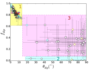
Figure 3: Plot of dipolarity $f_{dip}$ versus dipole tile angle $\theta_{dip}$ for the numerical models discussed here. The colour of the symbol rim represents the background density profile of the model (black: BG-G14, yellow: polytrope $N_{\rho}\!=\!4$, cyan: polytrope $N_{\rho}\!=\!5$). The face colour of the symbols corresponds to agreement with VIP4 quantified by $M$  white corresponds to $\mbox{$M$}\!>\!0.12$, lighter grey corresponds to $0.08\!\leq\!\mbox{$M$}\!\leq\!0.12$ and darker grey to $\mbox{$M$}\!\leq\!0.08$ (see Eq. 29). The red ’$\times$’ and blue ’+’ symbols show the VIP4 and JCF Jupiter field models, respectively. The red-rimmed triangle is the G14’s solution while the magenta-rimmed triangle corresponds to one simulation by Heimpel and Gómez-Pérez (2011). The shape of the symbols indicates the Ekman number ($E\!=\!10^{-4}$ - circles, $E\!=\!3\times 10^{-5}$ - squares, $E\!=\!10^{-5}$ - triangles). Error bars illustrate the time variability and show the standard deviation for values larger and smaller than the mean independently.

Figure 3 compares dipolarity and dipole tilt of the numerical models with VIP4, JCF. The solutions fall into the three distinct regimes introduced by Duarte et al. (2013). Regime $1$, indicated by a yellow box, is characterized by dynamos with a strong axial dipole component and generally weaker zonal flows. Regime $2$, the cyan box, encompasses cases where the axial dipole contribution remains typically weak. Finally, regime $3$, the magenta box, contains models where the axial dipole contribution varies strongly in time, as indicated by the larger error bars. Solutions in regimes $2$ and $3$ typically have strong zonal flows. Several previously discovered reasons for a dynamo to end up in regime $1$ where Jupiter-like solutions can be expected have been discussed in the introduction. Our new simulations confirm the respective inferences and we provide a few examples in the following. In particular the competition between zonal flows and dipolar fields continues to play a decisive role.

The differences in the three density profiles considered here (see Fig. 1) have no effect on the ability of the dynamo to maintain a dipole-dominated field. The dynamics is mainly influenced by the density gradients which differ more significantly in the outer part of the shell. The profiles may thus indeed yield different flows in this region but the low conductivity layer required to guarantee dipole-dominated fields prevent them from affecting the dynamo.

When the low conductivity layer is too thick, however, the field becomes once more multipolar (Duarte et al., 2013). Our model $12$ with a transition radius of $\chi_{m}\!=\!70$% instead of $80$% or $90$% in the other cases is an example for this effect. The ‘early decaying’ conductivity profile (yellow line in Fig. 2) potentially also causes the same problem and most of the respective $E\!=\!10^{-4}$ models ($9$, $35$, $45-48$) and $E\!=\!10^{-5}$ models ($61$, $63-65$) indeed end up being multipolar. The remaining higher conducting region where Lorentz forces could counteract the Reynolds stresses that drive zonal winds simply becomes too small (Duarte et al., 2013). We come back to discussing the impact of the different conductivity profiles below.

The pairs of dipolar and multipolar cases $10/11$ and $29/30$ in Tab. LABEL:TabRes are examples for the bistability at not too large Rayleigh numbers and $Pr\!=\!1$, the former pair for a polytropic profile and the latter for a BG-G14 model. At larger Rayleigh numbers and $Pr\!=\!1$ only the multipolar branch remains, for example model $43$ is dipolar at $Ra/Ra_{cr}\!=\!7.4$ while only the multipolar dynamo $49$ is found at $Ra/Ra_{cr}\!=\!8.4$. The behaviour seems to be different at $Pr\!=\!0.1$ where we find only multipolar solutions for $Ra/Ra_{cr}\!=\!7.8$ (model $16$) to $Ra/Ra_{cr}\!=\!8.4$ (model $18$). Increasing $Ra$ further to $Ra/Ra_{c}\!=\!9.8$ in model $19$, however, establishes a dipole-dominated dynamo, a behaviour not observed for $Pr\!=\!1$. We have checked that dipolar solutions cannot exist at lower $Ra$ since our values in models $16-18$ represent the onset of dynamo action, but we have not checked at which $Ra$ value multipolar solution would reappear.

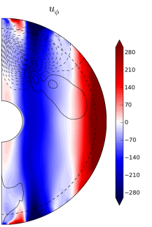
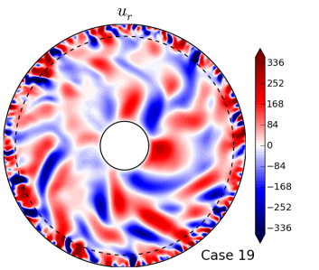
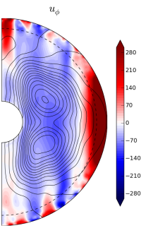
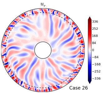
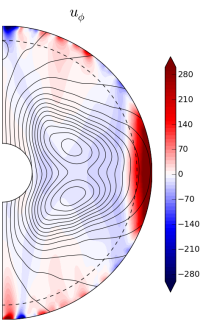
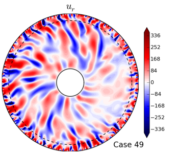
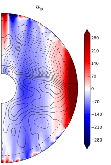
Figure 4: Radial flow of four models (one per row) in the equatorial plane (left column) and zonal flow with superimposed axisymmetric field lines (right column). Red (blue) indicates outward (inward) or prograde (retrograde) flows, respectively. The first two rows show cases with $Pr\!=\!0.1$ and the last two $Pr$ unity. The supercriticality is from top to bottom $7.8$, $9.7$, $5.7$, $8.4$. The dashed lines correspond to the $r_{m}$ parameter in the variable conductivity profile definition (see Eq. 3).

Figure 4 compares dipolar and multipolar simulations which differ only in Prandtl and Rayleigh number. The $Pr\!=\!1$ cases $26$ and $49$ ran at $Ra/Ra_{cr}\!=\!5.7$ and $Ra/Ra_{cr}\!=\!8.4$ while the $Pr\!=\!0.1$ models $16$ and $19$ have $Ra/Ra_{cr}\!=\!7.8$ and $Ra/Ra_{cr}\!=\!9.7$, respectively. The non-axisymmetric flows, illustrated with radial flow contours in the left column, are generally larger scale for $Pr\!=\!0.1$ than for $Pr\!=\!1$ as already predicted by the critical wave numbers (see Tab. 1). Note that the scale difference is more pronounced in the deeper region than in the weakly conducting outer shell delineated by a dashed line.

The smaller $Ra$ flows ($16$ and $26$) show larger differences with a much stronger increase of radial velocities for $Pr\!=\!1$. Also, the strong dipolar field at $Pr\!=\!1$ strongly suppresses the inner retrograde zonal jet (right column of Fig. 4. The faster non-axisymmetric deeper flows in the $Pr\!=\!0.1$ solution actually drive a surprisingly vigorous inner jet, much faster than even in a non-magnetic $Pr\!=\!1$ case (Gastine and Wicht, 2012).

Figure 4 shows that in addition to the strong geostrophic equatorial jet there are also shallower mid- to high-latitude zonal winds that remain confined to the weakly conducting region. These winds are somewhat more pronounced in the low Prandtl number simulations $16$ and $19$ but they are never much faster than the non-axisymmetric flow contributions. Moreover, while the equatorial jet is very persistent over the whole duration the mid- to high-latitude winds change on time scales only slightly longer than the typical time scale of the non-axisymmetric flows (of comparable length scale). Both type of zonal flows features therefore seem to obey different dynamics but further in-depth analysis is required clarify whether this may change at more realistic parameters.

For both Prandtl numbers, the radial gradient in non-axisymmetric flow velocities decreases with Rayleigh number. Both larger $Ra$ flows ($19$ and $49$) then seem rather similar. Except for the scale difference there is no apparent reason why only one of the two supports a dipole-dominated dynamo. We can only conclude that the competition between the dipolar field and Reynolds stress driven zonal winds is less severe for $Pr\!=\!0.1$ once the deeper flows become stronger at larger $Ra$.

Our new $Pr\!=\!1$ simulations confirm the trade-off between the Rayleigh number and the magnetic Prandtl described by various authors (Duarte et al., 2013; Schrinner et al., 2014; Jones, 2014; Raynaud et al., 2015): an increase in $Pm$ can prevent a dynamo from becoming multipolar, Cases $32$ to $34$ illustrate this effect: case $32$ is multipolar at $Pm_{i}\!=\!1$ while cases $33$ and $34$ are dipolar at $Pm_{i}\!=\!2$ and $Pm_{i}\!=\!3$, respectively. Cases $42$ and $43$ are another example where increasing $Pm_{i}$ from $1$ to $2$ proved successful. We expect that increasing $Pm$ should also extend the regime of dipolar dynamo action at $Pr\!=\!0.1$ as well at least to a certain degree.

All of our $9$ purely internally heated models are multipolar which confirms the conjecture by Jones (2014) that this driving mode favours complex magnetic field configurations. Even the choice of a small Prandtl number $Pr\!=\!0.1$ and a large magnetic Reynolds number of up to $Pm_{i}\!=\!8$ did not help to recover dipole-dominated dynamo action. Note that Jones (2014) normalizes $Pm$ by the mid-depth value while we use the inner boundary value.

Whether or not a lower Ekman number helps to stabilize dipole-dominated dynamo action is hard to conclude from our data set. Though we have ran cases at three different Ekman numbers they also often differ in the other system parameters, which makes it difficult to isolate the Ekman number effect. An indication may be that we now find two cases ($60$ and $62$) where an ’early decaying’ profile yields dipole-dominated dynamo action. This is far from being conclusive and additional simulations are required to clarify this point.

3.4 Dipolar models

We proceed with discussing how well the dipolar solutions replicate VIP4 or JCF. Figure 5a shows dipolarity and tilt for all models in regime $1$ and demonstrates that both are correlated in the sense that strongly dipolar models also tend to have lower tilts. At least to a large degree this correlation simply reflects the definition of the shown field characteristics. Both mean relative dipole contributions are already very similar to the VIP4 and JCF counterparts for many of our dipolar models. Dark symbols in Fig. 5 indicate particularly Jupiter-like models with $M$ values below $0.08$. The misfit values of all out models are listed in the last column Tab. LABEL:TabRes. The ’error’ ellipses spanned by the standard deviations for some of our best models actually include VIP4 and JCF which means that the respective Jupiter values are closely recovered at times. A slightly larger equatorial dipole would further reduce the average misfit. A tilt of $\theta\!\sim\!14^{\circ}$ marks the boundary between dipolar and multipolar dynamos which also seems to be true for geodynamo simulations (Wicht and Christensen, 2010). Jupiter’s dynamo seems to operate within that boundary as well.

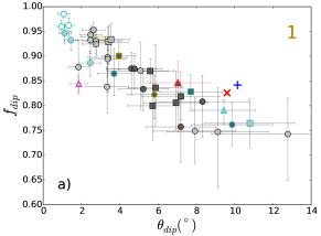
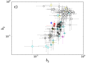
Figure 5: Top panel: axial dipole contribution $f_{dip}$ (related to $b_{10}$ through Eq. 23) and dipole tilt angle $\theta_{dip}$ (related to $b_{11}$ through Eq. 24) for the dipole-dominated solutions in regime $1$ of Fig. 3. The red ‘$\times$’ symbol corresponds to VIP4 and the blue ‘$+$’ to JCF. Symbols represent time averages while the error bars show standard deviations (see Fig. 3 for more explanation). Middle and bottom panels: axial dipole contribution $b_{10}$ and equatorial dipole contribution $b_{11}$ in the middle panel, and relative quadrupole $b_{2}$ and octupole contributions $b_{3}$ in he bottom panel.

Figures 5b,c show the relative quadrupole and octupole contributions, respectively, for all considered models. Multipolar cases reach values beyond $0.3$ and some come even close to equipartition at $b_{2}\!\approx\!b_{3}\!\approx\!0.4$, indicating comparable magnetic energy in each spherical harmonic degree. VIP4 or JCF values are once more inside the ’error ellipses’ for a number of our best models but a smaller relative octupole contribution would further improve the overall agreement. Note that the triangle for the G14 model lies particularly close to VIP4.

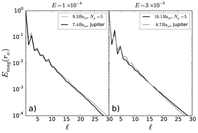
Figure 6: Magnetic spectra as a function of the spherical harmonic degree $\ell$ for two different density profiles and the G14 electrical conductivity model. Grey lines show simulations using the G14 density model while black lines indicate $N_{\rho}\!=\!5$ polytrope models. The left panel shows cases $8$ and $43$ with $E\!=\!10^{-4}$ and the right panel cases $14$ and $59$ with $E\!=\!3\times 10^{-5}$.

Figures 5b,c suggest that neither the Ekman numbers (symbol type) nor the background density models (rim colour) have a direct impact on how closely a dipole-dominated simulation replicates VIP4. Figure 6 demonstrates the similarity of the magnetic spectra for two dipolar solutions with a polytropic $N_{\rho}\!=\!5$ and the BG-G14 density at two different Ekman numbers. As discussed above, the electrical conductivity profiles chosen in this work likely reduce the potential impact of the density model.

The simulations reveal two other important effects that decisively influence the relative spectral contributions in our dipolar dynamo solutions. Several of our magnetic fields are actually too dipolar. The axial dipole contribution is so dominant that these models end up as a cluster in the upper left part of Fig. 5a and the lower left part of the bottom panel. Comparing, for example, models $4$ and $8$ in Tab. LABEL:TabRes illustrates this effect: while in model $4$ the axial dipole is far too dominant, increasing $Ra$ by $25$% leads to a very VIP4-like model $8$. In many cases we could identify a too small Rayleigh number as the reason. Another consequence of a smallish Rayleigh number is often a too simplistic time dependence which, however, is not considered here (Wicht and Christensen, 2010).

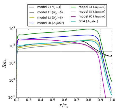
Figure 7: Convective magnetic Reynolds number profiles (Eq. 19) for seven new simulations are for G14. See Tab. 2 and Tab. LABEL:TabRes for more information on the model parameters and properties. The horizontal black line marks $Rm_{c}\!=\!50$ and the vertical dashed line $r/r_{o}\!=\!0.9$.

The second important factor that influences how close our simulations come to replicating Jupiter’s magnetic field is the electrical conductivity model. The combination of electrical conductivity and flow amplitude determines the magnetic Reynolds number profile $Rm_{c}(r)$ and thus the depth of the dynamo process. Since the flow profiles typically increase mildly with radius, it is mostly the decrease in $Rm_{c}$ that delimits the dynamo region. Figure 7 illustrates $Rm_{c}(r)$ for six of our best models ($2,11,13,20,44,56$) and one less successful example ($60$). We have added a horizontal line indicating the critical value $Rm\!=\!50$ where dynamo action becomes possible in Boussinesq simulations (Christensen and Aubert, 2006). The normalized radius beyond which $Rm_{c}$ remains below $50$ will be referred to as $R_{50}$ in the following: $Rm_{c}(r)\!<\!50\;\mbox{for}\;r/r_{o}\!\geq\!\mbox{$R_{50}$}$.

Most simulations that come closer to replicating VIP4 use the G14 electrical conductivity profile (cyan line in Fig. 2) like models $13$, $20$, $44$ and $56$ depicted in Fig. 7. The profiles for $13$, $56$, and $G14$ are very similar and all yield $\mbox{$R_{50}$}\!=\!r/r_{o}\!=\!0.9$. The high magnetic Prandtl number of $Pm_{i}\!=\!10$ in model $44$ leads to the largest magnetic Reynolds numbers of up to $Rm_{c}\!=\!1000$ in our simulations. The respective green profile in Fig. 7 illustrates that $R_{50}$ is pushed out to a particularly large value of $0.92$. The blue line shows model $20$, which ranks second in terms of $Rm$ amplitudes and has a slightly smaller $R_{50}$ value of $0.91$.

The magenta line in Fig. 7 shows the profile for model $62$ which uses the early decaying conductivity model (cyan line in Fig. 2). Dynamo action is then more concentrated at depth with a smallish $\mbox{$R_{50}$}\!=\!0.86$. Most of the simulations using this profile yield multipolar dynamos and those which remain dipolar (models $9,60,62$) have a too strong axial dipole and end up as white or light grey dots in the upper left corner of Fig. 5a and the lower left part of Fig. 5c. The reason is likely purely geometric: assuming that the field for radii $r\!>\!\mbox{$R_{50}$}$ is a potential field the individual spherical harmonic surface field contributions are by a factor $(\mbox{$R_{50}$}/r_{o})^{\ell+2}$ smaller than at $R_{50}$. The dominance of the dipole contribution thus increases with decreasing $R_{50}$.

Models using electrical conductivity profiles with a deeper transition radius, for example $\chi_{m}\!=\!80\%$ instead of $\chi_{m}\!=\!90\%$, face the same principal problem (models $1,2,3,5-7,11$ and $30,31,40$) but the decay rate naturally also plays a role. Models $2$ and $11$ use $\chi_{m}\!=\!80\%$ but combined with a mild conductivity drop of only two orders of magnitude (black line in in Fig. 2). Black and grey lines in Fig. 7 illustrate the respective $Rm_{c}$ profiles. The larger flow velocities in model $2$ push the dynamo region out to $\mbox{$R_{50}$}\!=\!0.89$ while $\mbox{$R_{50}$}\!=\!0.86$ in model $11$. Both actually have very favourable misfit values of $\mbox{$M$}\!=\!0.065$ and $\mbox{$M$}\!=\!0.067$, respectively, despite the fact that the electrical conductivity profiles are not very Jupiter-like. We will demonstrate below that higher harmonic field contributions should allow to dismiss these models.

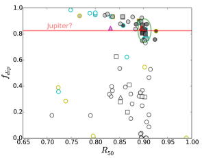
Figure 8: Relative axial dipole contribution plotted against $R_{50}$, the relative radius where the magnetic Reynolds number drops below $50$. See Fig. 5 for an explanation of the different symbols.

Figure 8 shows the dependence of the relative axial dipole contribution $b_{10}$ on $R_{50}$ for all analysed dynamo models. Model $56$ with $\mbox{$R_{50}$}\!=\!0.90$ and $\mbox{$b_{10}$}\!=\!0.12$ has the smallest misfit value of $\mbox{$M$}\!=\!0.061$. We generally regard the dark-coloured cases with $\mbox{$M$}\!\leq\!0.08$ as our ’best models’. They cluster around $\mbox{$R_{50}$}\!\approx\!0.9$ in the region marked by an ellipse in Fig. 8. However, since the two models with the largest values of $\mbox{$R_{50}$}\!=\!0.93$ (model $1$) and $\mbox{$R_{50}$}\!=\!0.92$ (model $44$) are among our most Jupiter-like cases the upper bound remains unclear. Exploring models with yet larger $R_{50}$ radii should clarify this point in the future.

Given the large internal magnetic Reynolds numbers in Jupiter, the weak conductivity decrease predicted for the metallic layer practically plays no role. However, our simulations for the slowly decaying conductivity profile that attempts to replicate this feature has shown that it strongly influences the numerical dynamo models. For the limited flow velocities in our dipolar models, the conductivity profile used by G14 and our best models seems to offer a good compromise.

Model	$N_{\rho}$	$E$	$\dfrac{Ra}{Ra_{cr}}$	$Pm_{i}$	$Pm_{V}$	$Pr$	$\begin{matrix}r_{50}\\ (\%)\end{matrix}$	$\begin{matrix}f_{dip}\\ \ell\leq 4\end{matrix}$	$\begin{matrix}\theta_{dip}\\ (^{\circ})\end{matrix}$	$\dfrac{B_{\,\ell=1,\,m=1}}{B_{\,\ell\leq 4}}$	$\dfrac{B_{\,\ell=2}}{B_{\,\ell\leq 4}}$	$\dfrac{B_{\,\ell=3}}{B_{\,\ell\leq 4}}$	$\begin{matrix}Lo(r_{o})_{\,\ell\leq 4}\\ 10^{-2}\end{matrix}$	$\begin{matrix}Lo\\ 10^{-2}\end{matrix}$	$\begin{matrix}Ro_{c}\\ 10^{-2}\end{matrix}$	$M$
VIP4	$\sim\!8$	$\sim\!5\!\times\!10^{-19}$	$-$	$-$	$-$	$-$	$-$	$0.83$	$9.6$	$0.152$	$0.232$	$0.244$	$-$	$-$	$-$	$-$
RID	$\sim\!8$	$\sim\!5\!\times\!10^{-19}$	$-$	$-$	$-$	$-$	$-$	$0.85$	$10.2$	$0.163$	$0.247$	$0.210$	$-$	$-$	$-$	$-$
$1$	$4$	$10^{-4}$	$5.5$	$4.0$	$2.06$	$1.0$	$92.6$	$0.82$	$5.8$	$0.091$	$0.199$	$0.319$	$0.134$	$0.93$	$1.57$	$0.067$
$2$	$4$	$3\!\times\!10^{-5}$	$5.6$	$2.0$	$1.03$	$1.0$	$89.1$	$0.90$	$4.0$	$0.066$	$0.165$	$0.227$	$0.101$	$0.53$	$0.75$	$0.065$
$8$	$5$	$10^{-4}$	$9.3$	$2.0$	$1.03$	$1.0$	$90.1$	$0.76$	$9.9$	$0.145$	$0.258$	$0.334$	$0.096$	$0.89$	$2.15$	$0.070$
$11$	$5$	$10^{-4}$	$9.3$	$2.0$	$1.03$	$1.0$	$85.8$	$0.87$	$3.7$	$0.069$	$0.165$	$0.283$	$0.135$	$0.96$	$2.08$	$0.067$
$13$	$5$	$3\!\times\!10^{-5}$	$9.2$	$1.5$	$0.96$	$1.0$	$90.4$	$0.83$	$7.7$	$0.125$	$0.185$	$0.316$	$0.048$	$0.44$	$1.02$	$0.061$
$20$	$\jupiter$	$10^{-4}$	$11.7$	$2.0$	$1.27$	$0.1$	$90.7$	$0.88$	$4.6$	$0.081$	$0.171$	$0.221$	$0.124$	$2.25$	$3.95$	$0.064$
$33$	$\jupiter$	$10^{-4}$	$6.1$	$2.0$	$1.27$	$1.0$	$89.6$	$0.83$	$5.2$	$0.087$	$0.157$	$0.328$	$0.110$	$0.89$	$1.55$	$0.077$
$39$	$\jupiter$	$10^{-4}$	$6.1$	$2.0$	$1.27$	$1.0$	$88.5$	$0.88$	$4.8$	$0.081$	$0.129$	$0.287$	$0.151$	$0.95$	$1.55$	$0.078$
$43$	$\jupiter$	$10^{-4}$	$7.4$	$2.0$	$1.27$	$1.0$	$89.7$	$0.81$	$8.3$	$0.139$	$0.191$	$0.306$	$0.084$	$0.83$	$1.93$	$0.074$
$44$	$\jupiter$	$10^{-4}$	$7.4$	$10.0$	$6.39$	$1.0$	$92.4$	$0.76$	$7.2$	$0.108$	$0.222$	$0.301$	$0.053$	$1.06$	$2.13$	$0.067$
$55$	$\jupiter$	$3\!\times\!10^{-5}$	$7.4$	$1.2$	$0.77$	$1.0$	$89.8$	$0.87$	$5.6$	$0.094$	$0.118$	$0.306$	$0.068$	$0.47$	$0.87$	$0.076$
$56$	$\jupiter$	$3\!\times\!10^{-5}$	$7.4$	$1.5$	$0.96$	$1.0$	$89.9$	$0.82$	$7.2$	$0.116$	$0.221$	$0.291$	$0.057$	$0.48$	$0.87$	$0.061$
$57$	$\jupiter$	$3\!\times\!10^{-5}$	$7.9$	$1.5$	$0.96$	$1.0$	$90.1$	$0.84$	$5.9$	$0.090$	$0.193$	$0.282$	$0.061$	$0.50$	$0.91$	$0.078$
$58$	$\jupiter$	$3\!\times\!10^{-5}$	$8.7$	$1.2$	$0.77$	$1.0$	$89.7$	$0.81$	$6.9$	$0.109$	$0.209$	$0.324$	$0.062$	$0.52$	$1.05$	$0.070$
$59$	$\jupiter$	$3\!\times\!10^{-5}$	$8.7$	$1.5$	$0.96$	$1.0$	$90.4$	$0.80$	$5.7$	$0.088$	$0.237$	$0.312$	$0.054$	$0.52$	$1.03$	$0.072$
G14	$\jupiter$	$10^{-5}$	$12.3$	$0.6$	$0.37$	$1.0$	$89.5$	$0.85$	$7.0$	$0.108$	$0.208$	$0.240$	$0.038$	$0.27$	$0.69$	$0.063$
CAJ	$\jupiter$	$2.5\!\times\!10^{-5}$	$-$	$6.2$	$1.06$	$0.1$	$-$	$0.91$	$7.4$	$0.123$	$0.206$	$0.155$	$-$	$-$	$-$	$0.053$

Table 2: Numerical models that best match the VIP4 observational model(Connerney et al., 1998), according to the results of Eq. 29. We also show the more recent model from Ridley (2012). For comparison purposes, the G14 model has also been included as well as the model and single snapshot in Fig.5c of Jones (2014).

The parameters and field characteristics of our $15$ best cases are listed in Table 2 along with the values for G14 and the observational models VIP4 and JCF (Tab. LABEL:TabRes provides an overview for all models). The relative axial dipole contributions (column $8$) of the selected numerical models closely resemble Jovian values and range between $92$% and $108$% of the VIP4 data. The other characteristics vary more strongly, the relative equatorial dipole (column $11$) between $43$% and $95$% , the relative quadrupole (column $12$) between $51$% and $111$% and the relative octupole between $91$% and $137$% of the respective VIP4 values. As already discussed above, relative equatorial dipole contributions or quadrupole contributions are on average somewhat smaller than the Jovian values while the octupole is larger, but the overall agreement is indeed very decent.

The fact that the best models have different Ekman numbers, Prandtl numbers, and background models once more illustrates that Jupiter-like solutions can be found over a broader range of parameters, at least when Rayleigh number and magnetic Prandtl number are adjusted accordingly.

We should point out that the axial dipole and octupole contributions have opposite signs both in our models and in VIP4. This means a stronger field concentration nearer the equator (latitudes between $\pm 45^{\circ}$) and weaker at higher latitudes toward the polar regions. We will come back to this discussion in the following.

3.5 Beyond the $M$ measure

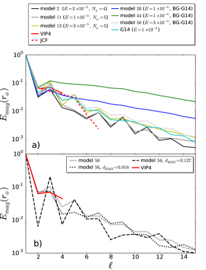
Figure 9: (a) Time-averaged surface field spectra for six of the best numerical models, and for G14 and VIP4. Line colours refer to the same models as in Fig. 7. More information on the models can be found in Tab. 2. (b) Comparison of spectra for the numerical model $56$ with VIP4 (red line). Model $56$ has the smallest mean $M$ value of all considered dynamos. While the grey solid line shows the mean spectrum for model $56$, dotted and dashed lines depict spectra for snapshots with particularly low (dotted) or large (dashed) $M$ values assumed during the model evolution.

So far we have discussed the Jupiter-likeness of our numerical simulations in terms of our misfit measure $M$ where only the first three spherical harmonics enter in an averaged sense. We now take a brief look at the higher harmonic contributions, at the time dependence, and at surface field maps.

Figure 9a shows the normalized magnetic power spectra up to degree $\ell\!=\!14$ for six of our best models, along with VIP4, JCF and G14. At least the $\ell\!=\!6$ and $7$ contributions in JCF are likely strongly controlled by the regularization and are not considered further. Though all the numerical models have similarly small $M$ values, four of the numerical spectra show distinct differences. Models $2$ and $11$ use the slowly decaying conductivity model (black line in in Fig. 2) which results in a mildly decaying magnetic Reynolds number profile (black and grey lines in Fig. 7). The respective spectra show particularly low $\ell\!=\!4$, $5$ and $6$ contributions which seem incompatible with the Jovian field.

The remaining numerical models use the same conductivity profile of G14. Models $20$ and $44$ reach particularly large magnetic Reynolds numbers which results in generally stronger higher harmonic contributions and an overall smoother spectrum. Already the $\ell\!=\!4$ contribution of model $44$ seems too high but model $20$ values are well acceptable.

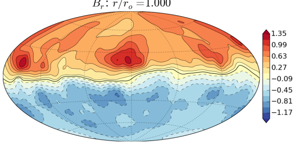
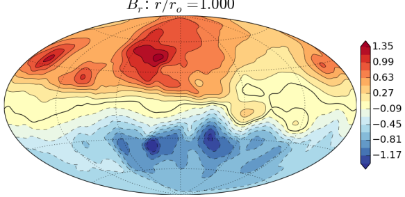
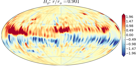
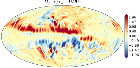
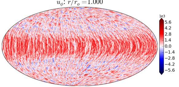
Figure 10: Radial magnetic field at the surface (top), azimuthal magnetic field at $R_{50}$ (middle) and azimuthal flow at the surface (bottom) for model $56$ snapshots with the particularly large (left) and low (right) $M$ values already depicted in Fig. 9b. Red (blue) depicts outward (inward) radial prograde (retrograde) magnetic field, respectively.

Figure 9b illustrates the time variability in the spectrum of model $56$ which has the lowest mean misfit $M$ among all examined simulations. During the model evolution, the misfit varies significantly between $0.012$ and $0.127$ around a mean of $\mbox{$M$}\!=\!0.061$. Dotted and dashed lines in Fig. 9b depict the spectrum for a particularly low value of $\mbox{$M$}\!=\!0.016$ and a large value of $0.127$ respectively. Figure 10 illustrates the respective magnetic field and zonal flow configurations. For the small misfit snapshot on the right, quadrupole and octupole contributions agree nearly perfectly with VIP4 while the larger misfit spectrum has a not very Jupiter-like zigzag structure. The lower panels in Fig. 10 depict the azimuthal flow at the outer boundary. The strong equatorial jet is clearly correlated with the banded structure, illustrating the importance of the $\Omega$-effect for the secondary dynamo operating in the transition region.

The magnetic fields show pronounced banded structures that are a result of the secondary dynamo discussed by G14: where the equatorial zonal flow jet reaches down to sizeable electrical conductivity values, strong azimuthal magnetic field bundles are created by the so-called $\Omega$-effect, i.e. shearing of radial field in azimuthal direction. Radial flows acting on these bundles in turn create strong surface field features at low to mid latitudes. While this process typically has a strong axisymmetric component, longitudinal variations in background magnetic field and radial flow can also lead to significant non-axisymmetric contributions. The strong zigzag structure in the large $M$ field spectrum can be traced back to a highly equatorially antisymmetric configuration with dominant axisymmetric and spherical harmonic order $m\!=\!2$ contributions. The axisymmetric contribution is mostly responsible for the relatively strong optupole field in our simulations. In VIP4 and JCF, on the other hand, the axisymmetric octupole is surprisingly weak. The Jupiter-like small misfit spectrum, on the other hand, is owed to a strong equatorially antisymmetric $m\!=\!1$ band structure which boosts $\ell\!=\!2$ and, to a smaller degree, also $\ell\!=\!4$ field contributions.

3.6 Rescaling to Jupiter conditions

Since there are several ways that the non-dimensional results can be rescaled to physical values, additional assumptions are required to overcome this non-uniqueness. For example, Jones (2014) assumes that the secular variation in the axial dipole component inferred by Ridley (2012) was correctly captured by his numerical dynamo model. This defines the time scale and ultimately leads to an estimated surface field that is about one order of magnitude too strong.

Theoretical considerations and extensive exploration of numerical dynamo simulations for a wide variety of set-ups suggest that the mean internal field strength as well as the mean convective velocity depend on the available convective power (Christensen and Aubert, 2006; Christensen et al., 2010; Aubert et al., 2009; Davidson, 2013; Yadav et al., 2013a, b). Support for the related scaling laws comes from the fact that they not only successfully predict the magnetic field strength of planets but also of some rapidly rotating fully convective stars (Christensen et al., 2009). Formulated in a non-dimensional framework (Yadav et al., 2013b), these laws show that the Lorentz number obeys

$$Lo\sim\sqrt{f_{Ohm}}\;1.08\,P^{*\,0.35}\textrm{,}$$ (30)

while the convective Rossby number for the non-axisymmetric flow contributions follows

$$Ro_{c}\sim 1.65\,P^{*\,0.42}\textrm{ .}$$ (31)

These scaling laws result from fitting power law dependencies to a number of dynamo simulations that also include anelastic models similar to the ones explored here (Yadav et al., 2013b) but only very few simulations with a weakly conducting outer layer. $P^{*}\!=\!P/(\Omega^{3}d^{2})$ is the dimensionless form of the convective power density $P$ (per mass) that can be approximated from the total surface heat flux density $F_{\jupiter}$ (per surface area) via

$$P=\frac{4\pi R_{\jupiter}^{2}\!F_{\jupiter}}{M_{\jupiter}}\,\int\frac{\alpha\,g}{c_{p}}dr\textrm{ .}$$ (32)

The factor $f_{Ohm}$ in Eq. 30 is the ratio of ohmic to total dissipation. Because of the small magnetic Prandtl number of planetary dynamo regions, ohmic dissipation clearly dominates so that $f_{Ohm}\!\approx\!1$. In the simulations where $Pm$ is typically around order one, $f_{Ohm}$ is smaller and typically varies around $f_{Ohm}\!\approx\!0.13$ in our simulations. The limited spread in $Pm$ explored in numerical variations also means that the related scaling exponent is hard to constrain.

Figure 11: Rossby number (a) and compensated Lorentz number (b) plotted against the dimensionless power for the models listed in Tab. 2. The grey dashed line corresponds to the scaling law (Eq. 30, the black dot-dashed line and green dotted show polynomial fits to our best models with fixed exponents (see text for more explanation). Panel (c) shows the ratio of surface Lorentz number $Lo_{o}$ to $Lo$ when considering the surface field up to spherical harmonic degree and order four (dark grey symbols) or degree and order $15$ (light grey symbols), representing the VIP4 and the expected Juno resolutions, respectively.

Figure 11 demonstrates that our best dynamo simulations follow these two scaling laws (dashed grey lines). The flow velocities are somewhat larger than suggested by Eq. 31 which we attribute to the larger flow velocities in the weakly conducting outer layer. To account for this differences, we varied the prefactor in the scaling law and found a best fit to our simulation results for a value of $1.97$ instead of $1.65$. An equivalent fitting for the magnetic field strength suggests a slightly larger prefactor of $1.17$ instead of $1.08$ for the Lorentz number (see black dashed line in Fig. 11).

Davidson (2013) derives a slightly different scaling based on theoretical considerations, mostly the fact that dynamos likely operate in a regime where Lorentz force, Coriolis force, buoyancy and pressure gradient balance in the Navier-Stokes equation. The scalings suggested for Lorentz and total Rossby number are then $Ro\!\sim\!P^{*\,4/9}$ and $Lo\!\sim\!P^{*\,1/3}$. Taking $Ro_{c}$ instead of $Ro$ to eliminate the contribution of the zonal flow, we fit the suggested scaling laws to our most Jupiter-like solutions. This yields prefactors of $2.63$ for $Ro$ and $0.96$ for $Lo$ (see green dotted line in Eq. 31).

When using the estimate of $5.5\,$W/m² for the surface heat flux density Hanel et al. (1981) and the interior model by French et al. (2012), the scaling laws Eq. 30 and Eq. 31 predict values of $Ro_{c,\jupiter}\!=\!3.36\times 10^{-6}$ and $Lo_{\jupiter}\!=\!1.95\times 10^{-5}$, respectively. This translates to a reasonable rms magnetic field strength of $7\,$mT and a rms convective velocity of $3\,$cm/s as already discussed by G14. Using the adjusted prefactors translates into a $23$% higher flow velocity and a $16$% higher field strength which are only marginal adjustments when considering the uncertainties in the scaling procedure. The alternative scaling suggested by Davidson (2013) yields an rms field strength of $12\,$mT and a rms convective velocity of $1\,$cm/s.

In order to compare the rms field strength with measurements of Jupiter’s surface field, we have to establish how both are related. Figure 11c shows the ratio of the surface Lorentz number

$$Lo_{o}=\left(\;\frac{E}{Pm_{i}}\frac{B_{o}^{2}}{\tilde{\rho}_{o}}\;\right)^{1/2}\textrm{,}$$ (33)

filtered at $\ell_{max}\!=\!4$, to the value of $Lo\,\rho^{1/2}$ expected if the density dependence would provide the only radial variation. The ratio ranges between $0.05$ and $0.20$ with a value of $0.14$ for G14. The scaling Eq. 30 would thus predict a rms surface field strength of $0.98\,$mT for G14 which is about $40$% higher than the VIP4 of JCF value of $0.68\,$mT. However, the ratio of $0.10$ required to reproduce the observational field strength lies within the range of our models. Similar inferences hold when using the Davidson (2013) scaling. Figure 11c demonstrates that the surface field strength increases by a maximum of $20$% when increasing the resolution from the VIP4 values (degree and order $4$, dark grey symbols) to the expected Juno value (degree and order $15$, light grey symbols).

The scaling predictions for the rms flow velocity between $1\,$cm/s and $10\,$cm/s agrees with similar estimates from other authors (Vasavada and Showman, 2005; Christensen and Aubert, 2006; Jones, 2014). Applying the same scaling to the zonal flow velocity, however, yields a much too low value. Gastine and Wicht (2012) demonstrate that the zonal flow velocity is determined by a balance between Reynolds stress and viscous drag. The latter is too large in the simulations in order to suppress the small scale dynamics that cannot be resolved with the available numerical power. Larger relative zonal flow velocities that would more clearly dominate the convective flow would require using lower Ekman numbers which would considerably increase the numerical costs.

4 Discussion and Conclusion

Our numerical simulations demonstrate that Jupiter’s magnetic field in the pre-Juno era can be explained by a variety of models. Successful models require a steep density and electrical conductivity decrease in the outer envelope similar to predictions from interior models. While the details of the density profile hardly matter, the conductivity profile is much more influential, mainly because it determines the depth of the dynamo region. As a working hypothesis we assume that dynamo action starts at the relative radius $R_{50}$ where the convective magnetic Reynolds number exceeds $50$, a critical value for self consistent numerical dynamo action in Boussinesq models (Christensen and Aubert, 2006). Jupiter-like models with realistic relative axial dipole, equatorial dipole, quadrupole and octupole field contributions are those where $R_{50}$ corresponds to roughly $90$% of the planetary radius. While smaller values below $\mbox{$R_{50}$}\!=\!0.85$ can be excluded with some confidence larger values however remain possible.

Assuming a rms non-axisymmetric velocity of $3\,$cm/s (G14) and the electrical conductivity profile suggested by (French et al., 2012) yields convective magnetic Reynolds numbers of more than $10^{6}$ at depth and $\mbox{$R_{50}$}\!\approx\!0.95$ for Jupiter. Because of the generally large flow velocities the top of the dynamo region necessarily lies in the regime where the electrical conductivity decreases very steeply and its exact location is rather insensitive to the flow amplitude. Assuming, for example, a ten times larger velocity of $30\,$cm/s would only change $R_{50}$ to $0.965$.

Since we have not really explored many larger $R_{50}$ values in our Jupiter-like simulations we can only estimate how such a value would affect the numerical models. Assuming a potential field beyond the top of the dynamo region at $\mbox{$R_{50}$}\!=\!0.90$ we have calculated the surface field spectrum for G14 at alternative values of $\mbox{$R_{50}$}\!=\!0.87$ and $\mbox{$R_{50}$}\!=\!0.95$ based on the scaling factor $(\mbox{$R_{50}$}/0.90)^{2\ell+4}$. Figure 12 demonstrates that raising the top of the dynamo region further boosts the already large octupole contributions in our simulations. On the other hand, the relative quadrupole and $\ell\!=\!4$ contributions are now closer to VIP4 values and the misfit changes only slightly. This misfit value is thus not sensitive enough to distinguish between models with $R_{50}\!>\!0.9$. For the deeper dynamo region, the $\ell\!=\!4$ contribution becomes much too low. An adjustment in Rayleigh number could compensate these effects to some degree.

Since the impact of $R_{50}$ grows with spherical harmonic degree $\ell$, the high resolution Juno results will allow to constrain the depth of the dynamo region much better than VIP4. Assuming a white spectrum for $\ell\!>\!4$ at $R_{50}$ leads to the predicted spectra shown in Fig. 12. At $\ell\!=\!20$ the differences between the $\mbox{$R_{50}$}\!=\!0.90$ and $\mbox{$R_{50}$}\!=\!0.95$ spectra amount to more than an order of magnitude. We note that the respective G14 spectra show a somewhat different tilt which also depends on the $\ell$ range. This suggests that the G14 spectrum is not really white at the top of the dynamo region, a topic that deserved to be addressed in more detail.

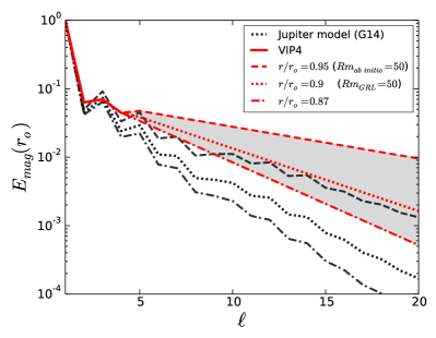
Figure 12: Magnetic power spectra for G14 (black), and VIP4 (red). In order to anticipate the possible high degree power spectrum, VIP4 has been extended by assuming a potential field above the top of the dynamo region at $0.95R_{\jupiter}$ (red dashed), $0.90R_{\jupiter}$ (red dotted) and $0.87R_{\jupiter}$ (red dashed-dotted), respectively. The field at the top of the dynamo region is supposed to be white for $\ell\!>\!4$. The solid black line shows the G14 spectrum at $\mbox{$R_{50}$}\!=\!0.90$. Assuming that this would really represent the top of the dynamo we have calculated alternative spectra for $0.87R_{\jupiter}$ (black, dash-dotted) and $0.95R_{\jupiter}$ (black, dashed).

The secondary dynamo due to the equatorial jet can produce strong magnetic bands at low to mid-latitudes on both sides of the equator. The magnetic field agrees more convincingly with the VIP4 model (Connerney et al., 1998) when these features are concentrated in one hemisphere. Juno’s measurement should be able to resolve these features that allow to constrain the deep zonal jet dynamics.

The unrealistically small magnetic Reynolds numbers in the simulations are unsatisfactory. While values of up to $Rm\!=\!10^{6}$ are expected for Jupiter’s interior, our numerical models only reach $1000$.

The simulations indicate that a larger $Rm$ tends to boost higher field harmonics beyond $\ell\!=\!3$ which suggest another feature that should be constrained by the Juno mission.

Larger $Rm$ values could be reached by either increasing the magnetic Prandtl number $Pm$ or the Rayleigh number. Planetary dynamos are characterized by magnetic Prandtl numbers much smaller than unity which means that Ohmic diffusion clearly dominates viscous diffusion. Since $Pm_{i}$ is already larger than unity in our simulations, increasing it even further seems like the wrong way to go. Increasing the Rayleigh number, on the other hand, always bears the danger of venturing into the multipolar regime unless the Ekman number is decreased accordingly (Christensen and Aubert, 2006). Since both larger $Ra$ and smaller $E$ lead to smaller spatial scales and shorter time steps, the numerical costs prevented us from following this approach further.

Our attempts to explore the dependence on the Ekman number and on the heating mode remain inconclusive. Lower Ekman numbers indeed seem to promote large scale field production in Boussinesq dynamos because of the stronger Coriolis force that helps to organize the flow (Christensen and Aubert, 2006). However, our database is still too limited to confirm a similar effect in anelastic simulations. All our nine fully internally heated simulations ended up as multipolar dynamos. This issue was already reported by Jones (2014) who nevertheless found a few Jupiter-like internally heated cases. A special combination of a low Ekman number, a low Prandtl number and a stronger concentration of heat sources at depth may have helped in his model. The difficulties in finding dipole-dominated solutions with internal heating seem remarkable since this is the more realistic driving scenario for Jupiter’s internal dynamo. We can only speculate that the problem may vanish at more realistic parameters, for example at lower Ekman numbers.

Sreenivasan and Jones (2006) and Simitev and Busse (2009) show that at low Rayleigh numbers large $Pr$ Boussinesq dynamos are dipole-dominated while small $Pr$ dynamos are multipolar. Our anelastic simulations seem to confirm this but also indicate that the small $Pr$ dynamos become dipole-dominated at larger Rayleigh numbers. Decreasing the Prandtl number below the $Pr\!=\!0.1$ value may thus help to reconcile dipole-dominated dynamo with internal heating.

Table 3: Summary of the time-averaged results. The grey-coloured rows correspond to dipole-dominated cases. In the column ‘$BC$’, the cases with octupole entropy at both boundaries are represented by $S\!S$ and the cases with fixed flux at both boundaries are represented by $F\!F$. The supercriticality of each model in column $Ra/Ra_{cr}$ is calculated using the values of $Ra_{cr}$ listed in Tab. 1.

Model	$N_{\rho}$	$\begin{matrix}E\\ 10^{-5}\end{matrix}$	$\dfrac{Ra}{Ra_{cr}}$	$Pr$	$Pm_{i}$	$Pm_{V}$	$a/\sigma_{m}/\chi_{m}$	$H$	$BC$	$\begin{matrix}f_{dip}\\ (\ell_{max}\!=\!4)\end{matrix}$	$\begin{matrix}\theta_{dip}\\ (^{\circ})\end{matrix}$	$\dfrac{B_{\,\ell=2}}{B_{\,\ell\leq 4}}$	$\dfrac{B_{\,\ell=3}}{B_{\,\ell\leq 4}}$	$Ro_{zon}$	$Rm_{c}$	$\Lambda$	$\begin{matrix}r_{50}\\ (\%)\end{matrix}$	$M$
$1$	$4$	$10$	$5.5$	$1.0$	$4.0$	$2.05$	$9./0.500/80$	$1.0$	$S\!S$	$8.22\!\times\!10^{-1}$	$5.8$	$0.199$	$0.319$	$1.15\!\times\!10^{-2}$	$156$	$2.04$	$92.6$	$0.067$
$2$	$4$	$3$	$5.6$	$1.0$	$2.0$	$1.03$	$9./0.500/80$	$1.0$	$S\!S$	$9.00\!\times\!10^{-1}$	$4.0$	$0.165$	$0.227$	$6.65\!\times\!10^{-3}$	$115$	$0.99$	$89.1$	$0.065$
$3$	$5$	$10$	$7.4$	$1.0$	$2.0$	$1.02$	$9./0.500/80$	$1.0$	$S\!S$	$9.32\!\times\!10^{-1}$	$1.4$	$0.077$	$0.229$	$1.41\!\times\!10^{-2}$	$63$	$0.63$	$83.3$	$0.106$
$4$	$5$	$10$	$7.4$	$1.0$	$2.0$	$1.27$	$13./0.200/90$	$1.0$	$S\!S$	$8.86\!\times\!10^{-1}$	$2.5$	$0.102$	$0.300$	$1.47\!\times\!10^{-2}$	$80$	$0.62$	$89.2$	$0.096$
$5$	$5$	$10$	$7.4$	$1.0$	$2.0$	$0.99$	$17./0.500/80$	$1.0$	$S\!S$	$9.47\!\times\!10^{-1}$	$1.1$	$0.058$	$0.207$	$1.92\!\times\!10^{-2}$	$51$	$0.36$	$80.0$	$0.117$
$6$	$5$	$10$	$7.4$	$1.0$	$2.0$	$0.98$	$25./0.500/80$	$1.0$	$S\!S$	$9.60\!\times\!10^{-1}$	$1.0$	$0.048$	$0.178$	$1.98\!\times\!10^{-2}$	$48$	$0.30$	$78.9$	$0.126$
$7$	$5$	$10$	$7.4$	$1.0$	$2.0$	$1.00$	$40./0.500/80$	$1.0$	$S\!S$	$9.62\!\times\!10^{-1}$	$1.3$	$0.053$	$0.163$	$2.06\!\times\!10^{-2}$	$48$	$0.29$	$80.0$	$0.125$
$8$	$5$	$10$	$9.3$	$1.0$	$2.0$	$1.27$	$13./0.200/90$	$1.0$	$S\!S$	$7.62\!\times\!10^{-1}$	$9.9$	$0.258$	$0.334$	$1.53\!\times\!10^{-2}$	$114$	$1.08$	$90.1$	$0.070$
$9$	$5$	$10$	$9.3$	$1.0$	$2.5$	$0.60$	$1./0.030/90$	$1.0$	$S\!S$	$9.85\!\times\!10^{-1}$	$1.1$	$0.052$	$0.083$	$2.46\!\times\!10^{-2}$	$39$	$0.48$	$74.9$	$0.144$
$10$	$5$	$10$	$9.3$	$1.0$	$2.0$	$1.03$	$9./0.500/80$	$1.0$	$S\!S$	$6.23\!\times\!10^{-1}$	$19.6$	$0.408$	$0.289$	$2.16\!\times\!10^{-2}$	$87$	$0.39$	$86.5$	$0.138$
$11$	$5$	$10$	$9.3$	1.0	$2.0$	$1.03$	$9./0.500/80$	$1.0$	$S\!S$	$8.65\!\times\!10^{-1}$	$3.7$	$0.165$	$0.283$	$1.55\!\times\!10^{-2}$	$81$	$1.00$	$85.8$	$0.067$
$12$	$5$	$10$	$11.2$	$1.0$	$2.0$	$0.69$	$9./0.500/70$	$1.0$	$S\!S$	$3.57\!\times\!10^{-1}$	$43.7$	$0.461$	$0.509$	$3.92\!\times\!10^{-2}$	$51$	$0.21$	$72.4$	$0.283$
$13$	$5$	$3$	$9.2$	$1.0$	$1.5$	$0.96$	$13./0.200/90$	$1.0$	$S\!S$	$8.28\!\times\!10^{-1}$	$7.7$	$0.185$	$0.316$	$1.05\!\times\!10^{-2}$	$129$	$0.64$	$90.4$	$0.061$
$14$	$5$	$3$	$16.1$	$1.0$	$1.0$	$0.64$	$13./0.200/90$	$1.0$	$S\!S$	$7.64\!\times\!10^{-1}$	$10.8$	$0.193$	$0.376$	$1.42\!\times\!10^{-2}$	$165$	$1.12$	$90.6$	$0.086$
$15$	$5$	$1$	$10.4$	$1.0$	$0.6$	$0.38$	$13./0.200/90$	$1.0$	$S\!S$	$7.91\!\times\!10^{-1}$	$9.4$	$0.126$	$0.397$	$1.11\!\times\!10^{-2}$	$140$	$0.33$	$90.5$	$0.099$
$16$	$\jupiter$	$10$	$7.8$	$0.1$	$2.0$	$1.27$	$13./0.200/90$	$1.0$	$S\!S$	$3.83\!\times\!10^{-2}$	$24.2$	$0.496$	$0.631$	$2.56\!\times\!10^{-2}$	$158$	$0.12$	$89.5$	$0.430$
$17$	$\jupiter$	$10$	$8.2$	$0.1$	$2.0$	$1.27$	$13./0.200/90$	$1.0$	$S\!S$	$3.32\!\times\!10^{-2}$	$37.0$	$0.476$	$0.625$	$2.75\!\times\!10^{-2}$	$162$	$0.20$	$89.4$	$0.432$
$18$	$\jupiter$	$10$	$8.4$	$0.1$	$2.0$	$1.27$	$13./0.200/90$	$1.0$	$S\!S$	$5.57\!\times\!10^{-3}$	$73.8$	$0.618$	$0.238$	$2.09\!\times\!10^{-2}$	$207$	$4.63$	$89.5$	$0.476$
$19$	$\jupiter$	$10$	$9.7$	$0.1$	$2.0$	$1.27$	$13./0.200/90$	$1.0$	$S\!S$	$8.98\!\times\!10^{-1}$	$3.4$	$0.139$	$0.218$	$2.78\!\times\!10^{-2}$	$206$	$4.85$	$89.4$	$0.087$
$20$	$\jupiter$	$10$	$11.7$	$0.1$	$2.0$	$1.27$	$13./0.200/90$	$1.0$	$S\!S$	$8.75\!\times\!10^{-1}$	$4.6$	$0.170$	$0.221$	$3.09\!\times\!10^{-2}$	$264$	$7.49$	$90.6$	$0.064$
$21$	$\jupiter$	$10$	$9.4$	$0.1$	$4.0$	$2.53$	$13./0.200/90$	$0.0$	$F\!F$	$1.83\!\times\!10^{-3}$	$84.1$	$0.602$	$0.216$	$1.73\!\times\!10^{-2}$	$247$	$3.75$	$90.4$	$0.483$
$22$	$\jupiter$	$10$	$9.4$	$0.1$	$8.0$	$5.05$	$13./0.200/90$	$0.0$	$F\!F$	$5.29\!\times\!10^{-1}$	$85.9$	$0.216$	$0.517$	$1.94\!\times\!10^{-2}$	$419$	$4.70$	$91.4$	$0.199$
$23$	$\jupiter$	$10$	$14.4$	$0.1$	$1.0$	$0.63$	$13./0.200/90$	$0.0$	$F\!F$	$1.70\!\times\!10^{-3}$	$88.5$	$0.750$	$0.145$	$2.33\!\times\!10^{-2}$	$97$	$1.41$	$89.5$	$0.515$
$24$	$\jupiter$	$10$	$14.4$	$0.1$	$2.0$	$1.27$	$13./0.200/90$	$0.0$	$F\!F$	$2.96\!\times\!10^{-3}$	$87.5$	$0.610$	$0.231$	$2.01\!\times\!10^{-2}$	$189$	$3.04$	$90.6$	$0.476$
$25$	$\jupiter$	$10$	$18.1$	$0.1$	$2.0$	$1.27$	$13./0.200/90$	$0.0$	$F\!F$	$1.25\!\times\!10^{-1}$	$87.0$	$0.482$	$0.416$	$3.29\!\times\!10^{-2}$	$211$	$2.49$	$90.6$	$0.392$
$26$	$\jupiter$	$10$	$5.7$	$1.0$	$2.0$	$1.27$	$13./0.200/90$	$1.0$	$S\!S$	$8.38\!\times\!10^{-1}$	$3.3$	$0.143$	$0.331$	$1.03\!\times\!10^{-2}$	$83$	$0.87$	$88.3$	$0.091$
$27$	$\jupiter$	$10$	$5.7$	$1.0$	$2.0$	$0.98$	$25./0.500/80$	$1.0$	$S\!S$	$1.74\!\times\!10^{-1}$	$79.5$	$0.646$	$0.441$	$1.63\!\times\!10^{-2}$	$54$	$0.20$	$79.0$	$0.387$
$28$	$\jupiter$	$10$	$5.7$	$1.0$	$2.0$	$1.20$	$36./0.500/85$	$1.0$	$S\!S$	$8.78\!\times\!10^{-1}$	$1.8$	$0.102$	$0.294$	$1.20\!\times\!10^{-2}$	$74$	$0.77$	$85.2$	$0.105$
$29$	$\jupiter$	$10$	$5.7$	$1.0$	$3.0$	$1.40$	$6./0.400/80$	$1.0$	$S\!S$	$3.21\!\times\!10^{-1}$	$87.4$	$0.498$	$0.435$	$1.41\!\times\!10^{-2}$	$84$	$0.35$	$83.2$	$0.303$
$30$	$\jupiter$	$10$	$5.7$	$1.0$	$3.0$	$1.40$	$6./0.400/80$	$1.0$	$S\!S$	$9.33\!\times\!10^{-1}$	$2.5$	$0.098$	$0.201$	$1.05\!\times\!10^{-2}$	$81$	$1.16$	$83.6$	$0.098$
$31$	$\jupiter$	$10$	$5.7$	$1.0$	$2.0$	$1.03$	$9./0.500/80$	$1.0$	$S\!S$	$9.44\!\times\!10^{-1}$	$2.5$	$0.092$	$0.189$	$1.06\!\times\!10^{-2}$	$64$	$0.84$	$82.0$	$0.098$
$32$	$\jupiter$	$10$	$6.1$	$1.0$	$1.0$	$0.63$	$13./0.200/90$	$1.0$	$S\!S$	$3.93\!\times\!10^{-1}$	$78.2$	$0.560$	$0.309$	$1.68\!\times\!10^{-2}$	$41$	$0.16$	$86.2$	$0.273$
$33$	$\jupiter$	$10$	$6.1$	$1.0$	$2.0$	$1.27$	$13./0.200/90$	$1.0$	$S\!S$	$8.34\!\times\!10^{-1}$	$5.2$	$0.157$	$0.328$	$1.03\!\times\!10^{-2}$	$91$	$0.97$	$89.6$	$0.077$
$34$	$\jupiter$	$10$	$6.1$	$1.0$	$3.0$	$1.92$	$13./0.200/90$	$1.0$	$S\!S$	$7.47\!\times\!10^{-1}$	$9.1$	$0.246$	$0.348$	$9.84\!\times\!10^{-3}$	$139$	$1.40$	$89.8$	$0.089$
$35$	$\jupiter$	$10$	$6.1$	$1.0$	$3.0$	$0.71$	$1./0.030/90$	$1.0$	$S\!S$	$1.75\!\times\!10^{-1}$	$67.7$	$0.723$	$0.307$	$1.95\!\times\!10^{-2}$	$38$	$0.11$	$71.0$	$0.402$
$36$	$\jupiter$	$10$	$6.1$	$1.0$	$2.0$	$0.89$	$3./0.250/85$	$1.0$	$S\!S$	$3.37\!\times\!10^{-1}$	$57.1$	$0.509$	$0.457$	$1.62\!\times\!10^{-2}$	$60$	$0.24$	$82.9$	$0.291$
$37$	$\jupiter$	$10$	$6.1$	$1.0$	$3.0$	$1.33$	$3./0.250/85$	$1.0$	$S\!S$	$9.31\!\times\!10^{-1}$	$2.8$	$0.112$	$0.195$	$1.02\!\times\!10^{-2}$	$90$	$1.31$	$87.8$	$0.092$
$38$	$\jupiter$	$10$	$6.1$	$1.0$	$2.0$	$0.99$	$4./0.110/90$	$1.0$	$S\!S$	$8.94\!\times\!10^{-1}$	$3.4$	$0.106$	$0.273$	$1.18\!\times\!10^{-2}$	$65$	$0.84$	$86.8$	$0.088$
$39$	$\jupiter$	$10$	$6.1$	$1.0$	$2.0$	$1.10$	$5./0.200/90$	$1.0$	$S\!S$	$8.75\!\times\!10^{-1}$	$4.8$	$0.129$	$0.287$	$1.00\!\times\!10^{-2}$	$77$	$0.94$	$88.5$	$0.078$
$40$	$\jupiter$	$10$	$6.1$	$1.0$	$2.0$	$1.03$	$9./0.500/80$	$1.0$	$S\!S$	$9.53\!\times\!10^{-1}$	$2.6$	$0.089$	$0.155$	$1.16\!\times\!10^{-2}$	$69$	$0.94$	$82.5$	$0.109$
$41$	$\jupiter$	$10$	$6.7$	$1.0$	$2.0$	$1.02$	$9./0.500/80$	$1.0$	$S\!S$	$3.97\!\times\!10^{-1}$	$82.9$	$0.480$	$0.392$	$1.69\!\times\!10^{-2}$	$79$	$0.43$	$83.4$	$0.260$
$42$	$\jupiter$	$10$	$7.4$	$1.0$	$1.0$	$0.63$	$13./0.200/90$	$1.0$	$S\!S$	$3.39\!\times\!10^{-1}$	$55.5$	$0.536$	$0.363$	$2.00\!\times\!10^{-2}$	$55$	$0.32$	$87.4$	$0.304$
$43$	$\jupiter$	$10$	$7.4$	$1.0$	$2.0$	$1.27$	$13./0.200/90$	$1.0$	$S\!S$	$8.08\!\times\!10^{-1}$	$8.3$	$0.191$	$0.306$	$1.17\!\times\!10^{-2}$	$119$	$1.45$	$89.7$	$0.074$
$44$	$\jupiter$	$10$	$7.4$	$1.0$	$10.$	$6.39$	$13./0.200/90$	$1.0$	$S\!S$	$7.57\!\times\!10^{-1}$	$7.2$	$0.222$	$0.301$	$3.65\!\times\!10^{-3}$	$565$	$7.29$	$92.4$	$0.067$
$45$	$\jupiter$	$10$	$7.4$	$1.0$	$4.0$	$1.00$	$1.1/0.020/90$	$1.0$	$S\!S$	$3.65\!\times\!10^{-1}$	$80.5$	$0.497$	$0.372$	$2.23\!\times\!10^{-2}$	$76$	$0.42$	$83.5$	$0.285$
$46$	$\jupiter$	$10$	$7.4$	$1.0$	$8.0$	$2.00$	$1.1/0.020/90$	$1.0$	$S\!S$	$2.63\!\times\!10^{-1}$	$71.2$	$0.490$	$0.441$	$1.80\!\times\!10^{-2}$	$159$	$1.06$	$87.6$	$0.311$
$47$	$\jupiter$	$10$	$7.4$	$1.0$	$10.$	$2.46$	$1.1/0.020/90$	$1.0$	$S\!S$	$1.51\!\times\!10^{-1}$	$69.4$	$0.553$	$0.477$	$1.66\!\times\!10^{-2}$	$188$	$1.28$	$87.4$	$0.394$
$48$	$\jupiter$	$10$	$8.4$	$1.0$	$4.0$	$1.00$	$1.1/0.020/90$	$1.0$	$S\!S$	$5.00\!\times\!10^{-1}$	$73.0$	$0.404$	$0.376$	$2.50\!\times\!10^{-2}$	$90$	$0.61$	$85.0$	$0.210$
$49$	$\jupiter$	$10$	$8.4$	$1.0$	$2.0$	$1.27$	$13./0.200/90$	$1.0$	$S\!S$	$2.49\!\times\!10^{-1}$	$69.3$	$0.488$	$0.462$	$1.54\!\times\!10^{-2}$	$140$	$1.13$	$89.7$	$0.320$
$50$	$\jupiter$	$10$	$5.1$	$1.0$	$8.0$	$5.11$	$13./0.200/90$	$0.8$	$S\!S$	$4.65\!\times\!10^{-1}$	$84.3$	$0.401$	$0.374$	$7.46\!\times\!10^{-3}$	$234$	$1.39$	$91.1$	$0.219$
$51$	$\jupiter$	$10$	$6.2$	$1.0$	$4.0$	$2.53$	$13./0.200/90$	$0.9$	$S\!S$	$3.28\!\times\!10^{-1}$	$54.7$	$0.464$	$0.434$	$1.04\!\times\!10^{-2}$	$161$	$0.97$	$89.4$	$0.277$
$52$	$\jupiter$	$10$	$6.2$	$1.0$	$6.0$	$3.77$	$13./0.200/90$	$0.8$	$S\!S$	$1.52\!\times\!10^{-1}$	$85.2$	$0.525$	$0.510$	$8.66\!\times\!10^{-3}$	$242$	$1.54$	$90.1$	$0.370$
$53$	$\jupiter$	$10$	$9.9$	$1.0$	$8.0$	$5.11$	$13./0.200/90$	$0.0$	$F\!F$	$1.80\!\times\!10^{-1}$	$44.9$	$0.489$	$0.454$	$1.44\!\times\!10^{-2}$	$153$	$0.03$	$91.1$	$0.337$
$54$	$\jupiter$	$10$	$11.8$	$1.0$	$8.0$	$5.11$	$13./0.200/90$	$0.0$	$F\!F$	$8.67\!\times\!10^{-2}$	$69.5$	$0.491$	$0.528$	$1.65\!\times\!10^{-2}$	$189$	$0.18$	$91.1$	$0.409$
$55$	$\jupiter$	$3$	$7.4$	$1.0$	$1.2$	$0.77$	$13./0.200/90$	$1.0$	$S\!S$	$8.70\!\times\!10^{-1}$	$5.6$	$0.118$	$0.306$	$7.79\!\times\!10^{-3}$	$98$	$0.57$	$89.8$	$0.076$
$56$	$\jupiter$	$3$	$7.4$	$1.0$	$1.5$	$0.96$	$13./0.200/90$	$1.0$	$S\!S$	$8.19\!\times\!10^{-1}$	$7.2$	$0.221$	$0.291$	$7.76\!\times\!10^{-3}$	$124$	$0.69$	$89.9$	$0.061$
$57$	$\jupiter$	$3$	$7.9$	$1.0$	$1.5$	$0.96$	$13./0.200/90$	$1.0$	$S\!S$	$8.36\!\times\!10^{-1}$	$5.9$	$0.193$	$0.282$	$8.17\!\times\!10^{-3}$	$131$	$0.73$	$90.1$	$0.078$
$58$	$\jupiter$	$3$	$8.7$	$1.0$	$1.2$	$0.77$	$13./0.200/90$	$1.0$	$S\!S$	$8.06\!\times\!10^{-1}$	$6.9$	$0.209$	$0.324$	$9.11\!\times\!10^{-3}$	$122$	$0.67$	$89.7$	$0.070$
$59$	$\jupiter$	$3$	$8.7$	$1.0$	$1.5$	$0.96$	$13./0.200/90$	$1.0$	$S\!S$	$8.00\!\times\!10^{-1}$	$5.7$	$0.237$	$0.312$	$8.81\!\times\!10^{-3}$	$152$	$0.89$	$90.4$	$0.072$
$60$	$\jupiter$	$3$	$9.6$	$1.0$	$3.0$	$0.74$	$1.1/0.015/90$	$1.0$	$S\!S$	$9.29\!\times\!10^{-1}$	$3.4$	$0.104$	$0.207$	$1.43\!\times\!10^{-2}$	$101$	$0.98$	$85.7$	$0.095$
$61$	$\jupiter$	$3$	$12.2$	$1.0$	$3.0$	$0.74$	$1.1/0.015/90$	$1.0$	$S\!S$	$4.09\!\times\!10^{-1}$	$65.6$	$0.472$	$0.353$	$1.84\!\times\!10^{-2}$	$148$	$0.66$	$87.0$	$0.250$
$62$	$\jupiter$	$3$	$10.2$	$1.0$	$3.0$	$0.74$	$1.1/0.015/90$	$0.9$	$S\!S$	$9.34\!\times\!10^{-1}$	$3.5$	$0.111$	$0.189$	$1.47\!\times\!10^{-2}$	$99$	$0.96$	$85.7$	$0.092$
$63$	$\jupiter$	$3$	$22.0$	$1.0$	$4.0$	$0.99$	$1.1/0.015/90$	$0.0$	$F\!F$	$6.26\!\times\!10^{-1}$	$41.0$	$0.339$	$0.373$	$1.71\!\times\!10^{-2}$	$59$	$0.06$	$84.3$	$0.142$
$64$	$\jupiter$	$3$	$23.7$	$1.0$	$4.0$	$0.99$	$1.1/0.015/90$	$0.0$	$F\!F$	$2.79\!\times\!10^{-1}$	$85.6$	$0.547$	$0.427$	$1.74\!\times\!10^{-2}$	$64$	$0.09$	$85.2$	$0.314$
$65$	$\jupiter$	$1$	$12.3$	$1.0$	$1.5$	$0.37$	$1.1/0.015/90$	$1.0$	$S\!S$	$3.15\!\times\!10^{-1}$	$89.8$	$0.546$	$0.349$	$1.43\!\times\!10^{-2}$	$102$	$0.16$	$85.2$	$0.319$
G14	$\jupiter$	$1$	$12.3$	$1.0$	$0.6$	$0.37$	$13./0.200/90$	$1.0$	$S\!S$	$8.46\!\times\!10^{-1}$	$7.0$	$0.208$	$0.240$	$9.54\!\times\!10^{-3}$	$124$	$-$	$89.5$	$0.063$

References

- Aubert et al. (2009) Aubert, J., Labrosse, S., Poitou, C., Dec. 2009. Modelling the palaeo-evolution of the geodynamo. Geophysical Journal International 179, 1414–1428.
- Braginsky and Roberts (1995) Braginsky, S. I., Roberts, P. H., 1995. Equations governing convection in earth’s core and the geodynamo. Geophysical and Astrophysical Fluid Dynamics 79, 1–97.
- Busse and Simitev (2006) Busse, F. H., Simitev, R. D., Oct. 2006. Parameter dependences of convection-driven dynamos in rotating spherical fluid shells. Geophysical and Astrophysical Fluid Dynamics 100, 341–361.
- Chabrier et al. (1992) Chabrier, G., Saumon, D., Hubbard, W. B., Lunine, J. I., Jun. 1992. The molecular-metallic transition of hydrogen and the structure of Jupiter and Saturn. ApJ 391, 817–826.
- Christensen and Wicht (2007) Christensen, U., Wicht, J., 2007. Numerical dynamo simulations. pp. 97–114.
- Christensen and Wicht (2015) Christensen, U., Wicht, J., 2015. Numerical dynamo simulations.
- Christensen (2001) Christensen, U. R., 2001. Zonal flow driven by deep convection in the major planets. Geophys. Res. Lett. 28, 2553–2556.
- Christensen and Aubert (2006) Christensen, U. R., Aubert, J., Jul. 2006. Scaling properties of convection-driven dynamos in rotating spherical shells and application to planetary magnetic fields. Geophysical Journal International 166, 97–114.
- Christensen et al. (2010) Christensen, U. R., Aubert, J., Hulot, G., Aug. 2010. Conditions for Earth-like geodynamo models. Earth and Planetary Science Letters 296, 487–496.
- Christensen et al. (2009) Christensen, U. R., Holzwarth, V., Reiners, A., Jan. 2009. Energy flux determines magnetic field strength of planets and stars. Nature 457, 167–169.
- Connerney et al. (1998) Connerney, J. E. P., Acuña, M. H., Ness, N. F., Satoh, T., Jun. 1998. New models of Jupiter’s magnetic field constrained by the Io flux tube footprint. J. Geophys. Res. 103, 11929–11940.
- Davidson (2013) Davidson, P. A., Oct. 2013. Scaling laws for planetary dynamos. Geophysical Journal International 195, 67–74.
- Duarte (2014) Duarte, L. D. V., 2014. Dynamics and Magnetic Field Generation in Jupiter and Saturn.
- Duarte et al. (2013) Duarte, L. D. V., Gastine, T., Wicht, J., Sep. 2013. Anelastic dynamo models with variable electrical conductivity: An application to gas giants. Physics of the Earth and Planetary Interiors 222, 22–34.
- Fortney and Nettelmann (2010) Fortney, J. J., Nettelmann, N., May 2010. The Interior Structure, Composition, and Evolution of Giant Planets. Space Sci. Rev. 152, 423–447.
- French et al. (2012) French, M., Becker, A., Lorenzen, W., Nettelmann, N., Bethkenhagen, M., Wicht, J., Redmer, R., Sep. 2012. Ab Initio Simulations for Material Properties along the Jupiter Adiabat. ApJS 202, 5.
- Gastine et al. (2012) Gastine, T., Duarte, L., Wicht, J., Oct. 2012. Dipolar versus multipolar dynamos: the influence of the background density stratification. A&A 546, A19.
- Gastine et al. (2014a) Gastine, T., Heimpel, M., Wicht, J., Jul. 2014a. Zonal flow scaling in rapidly-rotating compressible convection. Physics of the Earth and Planetary Interiors 232, 36–50.
- Gastine and Wicht (2012) Gastine, T., Wicht, J., May 2012. Effects of compressibility on driving zonal flow in gas giants. Icarus 219, 428–442.
- Gastine et al. (2014b) Gastine, T., Wicht, J., Duarte, L. D. V., Heimpel, M., Becker, A., Aug. 2014b. Explaining Jupiter’s magnetic field and equatorial jet dynamics. Geophys. Res. Lett. 41, 5410–5419.
- Gilman and Glatzmaier (1981) Gilman, P. A., Glatzmaier, G. A., Feb. 1981. Compressible convection in a rotating spherical shell. I - Anelastic equations. II - A linear anelastic model. III - Analytic model for compressible vorticity waves. ApJS 45, 335–388.
- Glatzmaier (1984) Glatzmaier, G. A., Sep. 1984. Numerical simulations of stellar convective dynamos. I - The model and method. Journal of Computational Physics 55, 461–484.
- Gómez-Pérez et al. (2010) Gómez-Pérez, N., Heimpel, M., Wicht, J., Jul. 2010. Effects of a radially varying electrical conductivity on 3D numerical dynamos. Physics of the Earth and Planetary Interiors 181, 42–53.
- Grodent et al. (2008) Grodent, D., Bonfond, B., GéRard, J.-C., Radioti, A., Gustin, J., Clarke, J. T., Nichols, J., Connerney, J. E. P., Sep. 2008. Auroral evidence of a localized magnetic anomaly in Jupiter’s northern hemisphere. Journal of Geophysical Research (Space Physics) 113, 9201.
-
Grote and Busse (2000)
Grote, E., Busse, F. H., Sep 2000. Hemispherical dynamos generated by
convection in rotating spherical shells. Phys. Rev. E 62, 4457–4460.
URL http://link.aps.org/doi/10.1103/PhysRevE.62.4457 - Hanel et al. (1981) Hanel, R., Conrath, B., Herath, L., Kunde, V., Pirraglia, J., Sep. 1981. Albedo, internal heat, and energy balance of Jupiter - Preliminary results of the Voyager infrared investigation. J. Geophys. Res. 86, 8705–8712.
- Heimpel et al. (2005) Heimpel, M., Aurnou, J., Wicht, J., Nov. 2005. Simulation of equatorial and high-latitude jets on Jupiter in a deep convection model. Nature 438, 193–196.
- Heimpel et al. (2016) Heimpel, M., Gastine, T., Wicht, J., Jan. 2016. Simulation of deep-seated zonal jets and shallow vortices in gas giant atmospheres. Nature Geoscience 9, 19–23.
- Heimpel and Gómez-Pérez (2011) Heimpel, M., Gómez-Pérez, N., Jul. 2011. On the relationship between zonal jets and dynamo action in giant planets. Geophys. Res. Lett. 38, 14201.
- Hess et al. (2011) Hess, S. L. G., Bonfond, B., Zarka, P., Grodent, D., May 2011. Model of the Jovian magnetic field topology constrained by the Io auroral emissions. Journal of Geophysical Research (Space Physics) 116, 5217.
- Hubbard (1975) Hubbard, W. B., Apr. 1975. Gravitational field of a rotating planet with a polytropic index of unity. Soviet Ast. 18, 621–624.
- Jones (2014) Jones, C. A., Oct. 2014. A dynamo model of Jupiter’s magnetic field. Icarus 241, 148–159.
- Jones et al. (2011) Jones, C. A., Boronski, P., Brun, A. S., Glatzmaier, G. A., Gastine, T., Miesch, M. S., Wicht, J., Nov. 2011. Anelastic convection-driven dynamo benchmarks. Icarus 216, 120–135.
- Jones et al. (2009) Jones, C. A., Kuzanyan, K. M., Mitchell, R. H., Aug. 2009. Linear theory of compressible convection in rapidly rotating spherical shells, using the anelastic approximation. Journal of Fluid Mechanics 634, 291.
- Kaspi et al. (2009) Kaspi, Y., Flierl, G. R., Showman, A. P., Aug. 2009. The deep wind structure of the giant planets: Results from an anelastic general circulation model. Icarus 202, 525–542.
- Lantz and Fan (1999) Lantz, S. R., Fan, Y., Mar. 1999. Anelastic Magnetohydrodynamic Equations for Modeling Solar and Stellar Convection Zones. ApJS 121, 247–264.
- Lian and Showman (2008) Lian, Y., Showman, A. P., Apr. 2008. Deep jets on gas-giant planets. Icarus 194, 597–615.
- Lowes (1966) Lowes, F. J., Apr. 1966. Mean-square values on sphere of spherical harmonic vector fields. Journal of Geophysical Research 71, 2179–2179.
- Lowes (1974) Lowes, F. J., Mar. 1974. Spatial power spectrum of the main geomagnetic field, and extrapolation to the core. Geophysical Journal International 36, 717–730.
- Matsui et al. (2016) Matsui, H., Heien, E., Aubert, J., Aurnou, J. M., Avery, M., Brown, B., Buffett, B. A., Busse, F., Christensen, U. R., Davies, C. J., Featherstone, N., Gastine, T., Glatzmaier, G. A., Gubbins, D., Guermond, J.-L., Hayashi, Y.-Y., Hollerbach, R., Hwang, L. J., Jackson, A., Jones, C. A., Jiang, W., Kellogg, L. H., Kuang, W., Landeau, M., Marti, P., Olson, P., Ribeiro, A., Sasaki, Y., Schaeffer, N., Simitev, R. D., Sheyko, A., Silva, L., Stanley, S., Takahashi, F., Takehiro, S.-i., Wicht, J., Willis, A. P., May 2016. Performance benchmarks for a next generation numerical dynamo model. Geochemistry, Geophysics, Geosystems 17, 1586–1607.
- Nettelmann et al. (2012) Nettelmann, N., Becker, A., Holst, B., Redmer, R., May 2012. Jupiter Models with Improved Ab Initio Hydrogen Equation of State (H-REOS.2). ApJ 750, 52.
- Olson et al. (1999) Olson, P., Christensen, U., Glatzmaier, G. A., May 1999. Numerical modeling of the geodynamo: Mechanisms of field generation and equilibration. J. Geophys. Res. 104, 10383–10404.
- Raynaud et al. (2015) Raynaud, R., Petitdemange, L., Dormy, E., Apr. 2015. Dipolar dynamos in stratified systems. MNRAS 448, 2055–2065.
- Ridley (2012) Ridley, V. A., 2012. Jovimagnetic Secular Variation. PhD thesis, Univ. of Liverpool, England, U. K.
- Ridley and Holme (2016) Ridley, V. A., Holme, R., Mar. 2016. Modeling the Jovian magnetic field and its secular variation using all available magnetic field observations. Journal of Geophysical Research (Planets) 121, 309–337.
- Sasaki et al. (2011) Sasaki, Y., Takehiro, S.-I., Kuramoto, K., Hayashi, Y.-Y., Oct. 2011. Weak-field dynamo emerging in a rotating spherical shell with stress-free top and no-slip bottom boundaries. Physics of the Earth and Planetary Interiors 188, 203–213.
- Schrinner et al. (2012) Schrinner, M., Petitdemange, L., Dormy, E., Jun. 2012. Dipole Collapse and Dynamo Waves in Global Direct Numerical Simulations. ApJ 752, 121.
- Schrinner et al. (2014) Schrinner, M., Petitdemange, L., Raynaud, R., Dormy, E., Apr. 2014. Topology and field strength in spherical, anelastic dynamo simulations. A&A 564, A78.
- Simitev and Busse (2009) Simitev, R. D., Busse, F. H., Jan. 2009. Bistability and hysteresis of dipolar dynamos generated by turbulent convection in rotating spherical shells. EPL (Europhysics Letters) 85, 19001.