Multiscale Projective Coordinates via Persistent Cohomology of Sparse Filtrations

Abstract.

We present in this paper a framework which leverages the underlying topology of a data set, in order to produce appropriate coordinate representations. In particular, we show how to construct maps to real and complex projective spaces, given appropriate persistent cohomology classes. An initial map is obtained in two steps: First, the persistent cohomology of a sparse filtration is used to compute systems of transition functions for (real and complex) line bundles over neighborhoods of the data. Next, the transition functions are used to produce explicit classifying maps for the induced bundles. A framework for dimensionality reduction in projective space (Principal Projective Components) is also developed, aimed at decreasing the target dimension of the original map. Several examples are provided as well as theorems addressing choices in the construction.

1. Introduction

Algebraic topology has emerged in the last decade as a powerful framework for analyzing complex high-dimensional data [2, 3]. In this setting, a data set is interpreted as a finite subset $X$ of an ambient metric space $(\mathbb{M},\mathbf{d})$; in practice $\mathbb{M}$ is usually Euclidean space, a manifold or a simplicial complex. If $X$ has been sampled from/around a “continuous” object $\mathbb{X}\subset\mathbb{M}$, the topology inference problem asks whether topological features of $\mathbb{X}$ can be inferred from $X$. On the one hand, this is relevant because several data science questions are reinterpretations of topological tests. To name a few: clustering is akin to finding the connected components of a space [4, 5]; coverage in a sensor network relates to the existence of holes [18, 11]; periodicity and quasiperiodicity are linked to nontrivial 1-cycles in time delay reconstructions [33, 31].

On the other hand, concrete descriptions of the underlying space $\mathbb{X}$ — e.g. via equations or as a quotient space — yield (geometric) models for the data $X$, which can then be used for simulation, prediction and hypothesis testing [25, 32]. When determining low-dimensional representations for an abstract data set, the presence of nontrivial topology heavily constraints the dimension and type of appropriate model spaces. The simplest example of this phenomenon is perhaps the circle, which is intrinsically 1-dimensional, but cannot be recovered on the real line without considerable distortion. Viral evolution provides another example; evolutionary trees are often inadequate models, as horizontal recombination introduces cycles [7]. The main goal of this paper is to show that one can leverage knowledge of the topology underlying a data set, e.g. determined via topological inference, to produce appropriate low-dimensional coordinates. In particular, we show how the persistent cohomology of a data set can be used to compute economic representations in real (or complex) projective spaces. These coordinates capture the topological obstructions which prevent the data from being recovered in low-dimensional Euclidean spaces and, correspondingly, yield appropriate representations.

Persistent (co)homology is one avenue to address the topology inference problem [38, 12]; it provides a multiscale description of topological features, and satisfies several inference theorems [30, 8, 10]. Going from a persistent homology computation to actionable knowledge about the initial data set, is in general highly nontrivial. One would like to determine: how are the persistent homology features reflected on the data? if the homology suggests a candidate underlying space $\mathbb{X}$, what is a concrete realization (e.g., via equations or as a quotient)? how does the data fit on/around the realization? At least three approaches have been proposed in the literature to address these questions: localization, homological coordinatization and circular coordinates.

For a relevant homology class, the idea behind localization is to find an appropriate representative cycle. This strategy is successful in low dimensions [15, 16], but in general even reasonable heuristics lead to NP-hard problems which are NP-hard to approximate [9]. Homological coordinatization [36] attempts to map a simplicial complex on the data to a simplicial complex with prescribed homology — a model suggested by a persistent homology computation. The map is selected by examining the set of chain homotopy classes of chain maps between the complex on the data and the model. Selecting an appropriate representative chain map, however, involves combinatorial optimizations which are difficult to solve in practice. Circular coordinates [13] leverages the following fact: there is a bijection $H^{1}(B;\mathbb{Z})\cong\big{[}B,S^{1}\big{]}$ between the 1-dimensional $\mathbb{Z}$-cohomology of a topological space $B$, and the set of homotopy classes of maps from $B$ to the circle $S^{1}$. When $B$ is a simplicial complex with the data as vertex set, this observation is used to turn 1-dimensional (persistent) $\mathbb{Z}/p$-cohomology classes for appropriate primes $p$, into circle-valued functions on the data.

The circular coordinates approach has been used successfully — for instance to parameterize periodic dynamics [14] — and is part of a bigger picture: if $G$ is an abelian group, $n\in\mathbb{Z}_{\geq 0}$ and $K(G,n)$ is an Eilenberg-MacLane space (i.e. its $n$-th homotopy group is $G$ and the others are trivial), then [26, Chapter 22, sec. 2]

$$H^{n}(B;G)\cong\big{[}B,K(G,n)\big{]}$$ (1)

In particular $K(\mathbb{Z},1)$ is homotopy equivalent to $S^{1}$; that is, $K(\mathbb{Z},1)\simeq S^{1}$. Since the bijection in (1) can be chosen so that it commutes with morphisms induced by maps of spaces (i.e. natural), using maps to other Eilenberg-MacLane spaces emerges as an avenue for interpreting persistent cohomology computations, and more importantly, to produce coordinates which leverage knowledge of the underlying topology. One quickly runs into difficulties as the next candidate spaces $K(\mathbb{Z}/2,1)\simeq\mathbb{R}\mathbf{P}^{\infty}$, $K(\mathbb{Z}/p,1)\simeq S^{\infty}/(\mathbb{Z}/p)$ (action via scalar multiplication on $S^{\infty}\subset\mathbb{C}^{\infty}$ by the $p$-th roots of unity) and $K(\mathbb{Z},2)\simeq\mathbb{C}\mathbf{P}^{\infty}$ are infinite. The purpose of this paper is to address the cases $\mathbb{R}\mathbf{P}^{\infty}$ and $\mathbb{C}\mathbf{P}^{\infty}$.

1.1. Approach

We use the fact that if $\mathbb{F}$ is $\mathbb{R}$ or $\mathbb{C}$, then $\mathbb{F}\mathbf{P}^{\infty}$ is the Grassmannian of 1-planes in $\mathbb{F}^{\infty}$ and — for a topological space $B$ — $\big{[}B,\mathbb{F}\mathbf{P}^{\infty}\big{]}$ can be naturally identified with the set of isomorphism classes of $\mathbb{F}$-line bundles over $B$ (Theorem 2.1). The isomorphism type of an $\mathbb{R}$-line bundle over $B$ is uniquely determined by its first Stiefel-Whitney class $w_{1}\in H^{1}(B;\mathbb{Z}/2)$, and the isomorphism type of a $\mathbb{C}$-line bundle over $B$ is classified by its first Chern class $c_{1}\in H^{2}(B;\mathbb{Z})$. These classes can be identified as elements of appropriate sheaf cohomology groups, and a classifying map $f:B\longrightarrow\mathbb{F}\mathbf{P}^{\infty}$ can be described explicitly from a Čech cocycle representative (Theorem 3.2). This links cohomology to $\mathbb{F}\mathbf{P}^{\infty}$-coordinates. For the case of point cloud data $X\subset(\mathbb{M},\mathbf{d})$, $B$ will be an open neighborhood of $X$ in $\mathbb{M}$, and we use the persistent cohomology of a sparse filtration on $X$ to generate appropriate Čech cocycle representatives (Theorem 7.4). Evaluating the resulting classifying map $f$ on the data $X$ produces another point cloud $f(X)\subset\mathbb{F}\mathbf{P}^{n}$. We develop in Section 5 a dimensionality reduction procedure for subsets of $\mathbb{F}\mathbf{P}^{n}$, referred to as Principal Projective Component Analysis. When this methodology is applied to the point cloud $f(X)\subset\mathbb{F}\mathbf{P}^{n}$, it produces a sequence of projections $P_{k}:f(X)\longrightarrow\mathbb{F}\mathbf{P}^{k}$, $k=1,\ldots,n$, each of which attempts to minimize an appropriate notion of distortion. The sets $P_{k}\circ f(X)$ are the $\mathbb{F}\mathbf{P}^{k}$-coordinates of $X$, for the Čech cocycle giving rise to $f$.

1.2. Organization

We end this introduction in Subsection 1.3 with a motivating data example. Section 2 is devoted to the theoretical preliminaries needed in later sections of the paper; in particular, we provide a terse introduction to vector bundles, the Čech cohomology of (pre)sheaves and the persistent cohomology of filtered complexes. In Sections 3 and 4 we prove the main theoretical results underlying our method. In particular, we show how singular cohomology classes yield explicit and computable maps to real (and complex) projective space. Sections 5, 6 and 7 deal with computational aspects. Specifically, section 5 develops Principal Projectives Components, a dimensionality reduction method in projective space, used to lower the target dimension of the maps developed in Sections 3 and 4. Section 6 deals with the problem of choosing cocycle representatives; we present theorems and examples which guide these choices. We end the paper in Section 7 showing how persistent cohomology can be used to make the approach practical for data sets with low intrinsic dimension.

1.3. Motivation and road map

Let us illustrate some of the ideas we will develop in this paper via an example. To this end, let $\mathbb{X}$ be the collection of intensity-centered $7\times 7$ grey-scale images depicting a line segment of fixed width, as show in Figure 1.

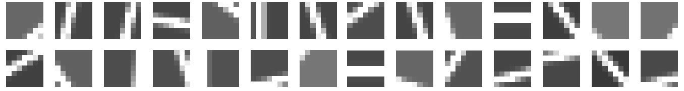
Figure 1. Typical elements in $\mathbb{X}$

By intensity-centered we mean that if the pixel values of $x\in\mathbb{X}$ are encoded as real numbers between -1 (black) and 1 (white), then the mean pixel intensity of $x$ is zero. We regard $\mathbb{X}$ as a subset of $\mathbb{R}^{49}$ by representing each image as a vector of pixel intensities, and endow it with the distance inherited from $\mathbb{R}^{49}$. A data set $X\subset\mathbb{X}$ is generated by sampling $1,682$ points. The thing to notice is that even when the ambient space for $\mathbb{X}$ is $\mathbb{R}^{49}$, the intrinsic dimensionality is low. Indeed, each image can be generated from two numbers: the angle of the line segment with the horizontal, and the signed distance from the segment to the center of the patch. This suggests that $\mathbb{X}$ is locally 2-dimensional.

Principal Component Analysis (PCA) [21] and ISOMAP [37] are standard tools to produce low-dimensional representations for data; let us see if we can use them to recover an appropriate 2-dimensional representation for $X$. Given the first $k$ principal components of $X$, calculated with PCA, their linear span $V_{k}$ is interpreted as the $k$-dimensional linear space which best approximates $X$. One can calculate the residual variance of this approximation, by computing the mean-squared distance from $X$ to $V_{k}$. Similarly, the fraction of variance from $X$ explained by $V_{k}$ is equal to difference between the variance of $X$ and the residual variance, divided by the variance of $X$. A similar notion can be defined for ISOMAP. We show in Figure 2(b) the fraction of variance, from $X$, recovered by PCA and ISOMAP

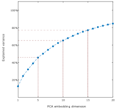
(a) PCA

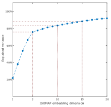
(b) ISOMAP

Figure 2. Explained variance, from $X$, versus embedding dimension.

Given the low intrinsic dimensionality of $\mathbb{X}$, it follows from the PCA plot that the original embedding $\mathbb{X}\hookrightarrow\mathbb{R}^{49}$ is highly non-linear. Moreover, the ISOMAP plot implies that even after accounting for the way in which $\mathbb{X}$ sits in $\mathbb{R}^{49}$, the data has intrinsic complexity that prevents it from being recovered faithfully in $\mathbb{R}^{2}$ or $\mathbb{R}^{3}$. That is, the data is locally simple (e.g. each $x\in X$ is described by angle and displacement) but globally complex. One possible source of said complexity is whether or not $\mathbb{X}$ is orientable; this is a topological obstruction to low-dimensional Euclidean embeddings. Using the observation that $\mathbb{X}$ is a manifold, its orientability can be determined from $X$ as we describe next. First, we construct a covering $\{B_{r}\}_{r=0}^{n}$ of $X$. From now on we will simplify the set notation $\{a_{\alpha}\}_{\alpha\in\Lambda}$ to $\{a_{\alpha}\}$ in the cases where the indexing set $\Lambda$ can be inferred from the context. Next, we apply Multi-Dimensional Scaling (MDS) [23] on each $B_{r}$ to get local Euclidean coordinates and, finally, we compute the determinant $\omega_{rt}=\pm 1$ associated to the change of local Euclidean coordinates on each $B_{r}\cap B_{t}$. If there is global agreement of local orientations (e.g., $\omega_{rt}$ =1 always), or local orientations can be reversed in the appropriate $B_{r}$’s so that the result is globally consistent (i.e. $\{\omega_{rt}\}$ is a coboundary: there exist $\nu_{r}$’s, with $\nu_{r}=\pm 1$, so that $\omega_{rt}=\nu_{t}/\nu_{r}$ for all $r,t=1,\ldots,n$), then $\mathbb{X}$ would be deemed orientable.

The cover for $X$ will be a collection of open balls centered at landmark data points selected through maxmin (also known as farthest point) sampling. That is, first one chooses an arbitrary landmark $\ell_{0}\in X$, and if $\ell_{0},\ldots,\ell_{r}$ have been determined, then $\ell_{r+1}\in X$ is given by

$$\ell_{r+1}=\operatorname*{\arg\!\max\;}_{x\in X}\big{(}\min\{\mathbf{d}(x,\ell_{0}),\ldots,\mathbf{d}(x,\ell_{r})\}\big{)}.$$

Here $\mathbf{d}$ is the geodesic distance estimate from the ISOMAP calculation. A finite number of steps of maxmin sampling results in a landmark set $\{\ell_{0},\ldots,\ell_{n}\}$ which tends to be well-distributed and well-separated across the data. For the current example we used $n=14$. Let $\epsilon_{0}=\cdots=\epsilon_{n}=9.3$ and

$$\mathcal{B}=\{B_{r}\}\;\;\mbox{ where }\;\;B_{r}=\{x\in X:\mathbf{d}(x,\ell_{r})<\epsilon_{r}\}$$

To put the radii $\epsilon_{r}$ in perspective, the distance between distinct $\ell_{r}$’s ranges from 4.5 to 14.6, and the mean pairwise distance is 9.5.

Let us now show how to calculate the determinant of the change of local coordinates. If $B_{r}\cap B_{t}\neq\emptyset$, let

$$f_{r}:B_{r}\longrightarrow\mathbb{R}^{2}\;\;\mbox{ and }\;\;f_{t}:B_{t}\longrightarrow\mathbb{R}^{2}$$

be the functions obtained from applying MDS on $\left(B_{r},\mathbf{d}\big{|}_{B_{r}}\right)$ and $\left(B_{t},\mathbf{d}\big{|}_{B_{t}}\right)$, respectively. If $\mathsf{O}(2)$ denotes the set of orthogonal $2\times 2$ real matrices, then the solution to the orthogonal Procrustes problem

$$\left(\Omega_{rt},\mathbf{v}_{rt}\right)\;\;=\operatorname*{\arg\!\min\;}_{\Omega\in\mathsf{O}(2),\;\mathbf{v}\in\mathbb{R}^{2}}\;\sum_{x\in B_{r}\cap B_{t}}\big{\|}f_{t}(x)-\big{(}\Omega\cdot f_{r}(x)+\mathbf{v}\big{)}\big{\|}^{2}$$

computed following [34], yields the best linear approximation to an isometric change of local ISOMAP coordinates. We let $\omega_{rt}:=\det(\Omega_{rt})$. In summary, we have constructed a finite covering $\mathcal{B}=\{B_{r}\}$ for $X$ and a collection of numbers $\omega_{rt}=\pm 1$ which, at least for this example, satisfy the cocycle condition: for all $0\leq r\leq n$ we have $\omega_{rr}=1$ and if $B_{r}\cap B_{s}\cap B_{t}\neq\emptyset$, then $\omega_{rs}\cdot\omega_{st}=\omega_{rt}$. In particular, a cohomology computation shows that $\{\omega_{rt}\}$ is not a coboundary and hence $\mathbb{X}$ is estimated to be non-orientable.

What we will see now, and throughout the paper, is that this type of cohomological feature can be further leveraged to produce useful coordinates for the data. Indeed (Theorem 3.2 and Corollary 3.4):
Theorem. For $\lambda\in\mathbb{R}$ let $\left|\lambda\right|_{+}=\max\{\lambda,0\}$, let $\mathbb{F}$ be either $\mathbb{R}$ or $\mathbb{C}$, and let $\mathbb{F}^{\times}=\mathbb{F}\smallsetminus\{\mathbf{0}\}$. For a metric space $(\mathbb{M},\mathbf{d})$ let $\{\ell_{0},\ldots,\ell_{n}\}\subset\mathbb{M}$ and fix positive real numbers $\epsilon_{0},\ldots,\epsilon_{n}$. If we let $\mathcal{B}=\{B_{r}\}$ with $B_{r}=\{b\in\mathbb{M}\,:\,\mathbf{d}(b,\ell_{r})<\epsilon_{r}\}$, $B=\bigcup\mathcal{B}$, and there is a collection $\omega=\{\omega_{rt}:B_{r}\cap B_{t}\longrightarrow\mathbb{F}^{\times}\}$ of continuous maps satisfying the cocycle condition (4), then $f_{\omega}:B\longrightarrow\mathbb{F}\mathbf{P}^{n}$ given in homogeneous coordinates by

$$f_{\omega}(b)=\bigg{[}\omega_{0j}(b)\cdot\left|\epsilon_{0}-\mathbf{d}(b,\ell_{0})\right|_{+}:\cdots:\omega_{nj}(b)\cdot\left|\epsilon_{n}-\mathbf{d}(b,\ell_{n})\right|_{+}\bigg{]}\;\;\;,\;\;\;b\in B_{j}$$ (2)

is well-defined (i.e. the value $f_{\omega}(b)$ is independent of the $j$ for which $b\in B_{j}$) and classifies the $\mathbb{F}$-line bundle on $B$ induced by $\big{(}\mathcal{B},\omega\big{)}$.
The preliminaries needed to understand this theorem will be covered in Section 2, and we will devote Section 3 to proving it. The map $f_{\omega}$ encodes in a global manner the local interactions captured by $\omega$, and the explicit formula allows us to map our data set $X\subset\mathbb{R}^{49}$ into $\mathbb{R}\mathbf{P}^{14}$ using the computed landmarks and determinants of local changes of coordinates. If we compute the principal projective components for $f_{\omega}(X)\subset\mathbb{R}\mathbf{P}^{14}$ (this will be developed in Section 5 as a natural extension to PCA in Euclidean space and of Principal Nested Spheres Analysis [22]), the profile of recovered variance shown in Figure 3 emerges:

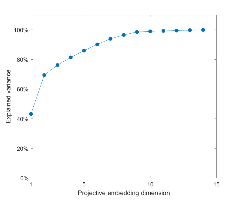
Figure 3. Recovered variance, from $f_{\omega}(X)\subset\mathbb{R}\mathbf{P}^{14}$, when projected onto principal projective subspace of given dimension.

From this plot we conclude that 2-dimensional projective space provides an appropriate reduction for $f_{\omega}(X)$. We show in Figure 4 said representation; that is, each image is placed in the $\mathbb{R}\mathbf{P}^{2}$ coordinate computed via principal projective component analysis on $f_{\omega}(X)$.

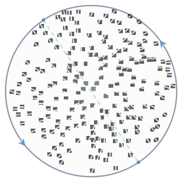
Figure 4. Some elements from $X$ placed on their computed $\mathbb{R}\mathbf{P}^{2}$-coordinates.

As the figure shows, the resulting coordinates recover the variables which we identified as describing points in $\mathbb{X}$: the radial coordinate in $\mathbb{R}\mathbf{P}^{2}$ corresponds to distance from the line segment to the center of the patch, and the angular coordinate captures orientation. Also, it indicates how $\mathbb{R}\mathbf{P}^{2}\cong\mathbb{X}$ parameterizes the original data set $X$.

Though the strategy employed in this example (i.e. local MDS + determinant of local change of coordinates) was successful, one cannot assume in general that the data under analysis has been sampled from/around a manifold. That said, the result from formula (2) only requires a covering $\mathcal{B}$ via open balls, and a collection of $\mathbb{F}^{\times}$-valued continuous functions $\omega=\{\omega_{rt}\}$ satisfying the cocycle condition. Given a finite subset $X$ of an ambient metric space $(\mathbb{M},\mathbf{d})$, one can always use maxmin sampling to produce a covering. We will show that any 1-dimensional (resp. 2-dimensional) $\mathbb{Z}/2$-cocyle (resp. $\mathbb{Z}$-cocycle) of the nerve complex $\mathcal{N}(\mathcal{B})$, for $\mathbb{F}=\mathbb{R}$ (resp. $\mathbb{F}=\mathbb{C}$), yields one such $\omega$ (Proposition 4.3 and Corollary 4.8). We also show that in dimension 1 (i.e., $\mathbb{F}=\mathbb{R}$) cohomologous cocycles yield equivalent projective coordinates, while in dimension 2 (i.e., $\mathbb{F}=\mathbb{C}$) the harmonic cocycle is needed (see Section 6).

It is entirely possible that a cohomology class reflecting sampling artifacts is chosen, as opposed to one associated to robust topological features of a continuous space $\mathbb{X}\subset\mathbb{M}$ underlying $X$. Here is where persistent cohomology comes in. Indeed, under mild connectivity conditions of $\mathcal{B}$, distinct cohomology classes yield maps to projective space with distinct homotopy types. Moreover, the maps resulting from a persistent class across its lifetime are compatible up to homotopy (Theorem 7.4 and Proposition 7.6). Hence, the result is a multiscale family of compatible maps which, for classes with long persistence, are more likely to reflect robust features of (neighborhoods around) $\mathbb{X}$.

The strategy outlined here is in fact a two-way street. One can use persistent cohomology to compute multiscale compatible projective coordinates, but the reserve is also useful: The resulting coordinates can be used to interpret the distinct persistent cohomology (= persistent homology) features of neighborhoods of the data, at least in cohomological dimensions 1 (with $\mathbb{Z}/2$ coefficients) and 2 (with $\mathbb{Z}/p$ coefficients for appropriate primes $p$).

2. Preliminaries

Vector Bundles

For a more thorough review please refer to [27]. Let $E$ and $B$ be topological spaces, and let $p:E\longrightarrow B$ be a surjective continuous map. The triple $\zeta=(E,B,p)$ is said to be a rank $k\in\mathbb{N}$ vector bundle over a field $\mathbb{F}$ (i.e. an $\mathbb{F}$-vector bundle) if each fiber $p^{-1}(b)$ is an $\mathbb{F}$-vector space of dimension $k$, and $\zeta$ is locally trivial. That is, for every $b_{0}\in B$ there exist an open neighborhood $U\subset B$ and a homeomorphism $\rho_{U}:U\times\mathbb{F}^{k}\longrightarrow p^{-1}(U)$, called a local trivialization around $b_{0}$, satisfying:

1. $p\left(\rho_{U}(b,\mathbf{v})\right)=b$ for every $(b,\mathbf{v})\in U\times\mathbb{F}^{k}$

2. $\rho_{U}(b,\cdot):\mathbb{F}^{k}\longrightarrow p^{-1}(b)$ is an isomorphism of $\mathbb{F}$-vector spaces for each $b\in U$

$E$ and $B$ are referred to as the total and base space of the bundle, and the function $p:E\longrightarrow B$ is called the projection map. Two vector bundles $\zeta=(E,B,p)$ and $\zeta^{\prime}=(E^{\prime},B,p^{\prime})$ are said to be isomorphic, $\zeta\cong\zeta^{\prime}$, if there exists a homeomorphism $T:E\longrightarrow E^{\prime}$ so that $p^{\prime}\circ T=p$ and for which each restriction $T|_{p^{-1}(b)}$, $b\in B$, is a linear isomorphism.

The collection of isomorphism classes of $\mathbb{F}$-vector bundles of rank $k$ over $B$ is denoted $\mathsf{Vect}_{\mathbb{F}}^{k}(B)$. An $\mathbb{F}$-vector bundle of rank $1$ is called an $\mathbb{F}$-line bundle, and the set $\mathsf{Vect}^{1}_{\mathbb{F}}(B)$ is an abelian group with respect to fiberwise tensor product of $\mathbb{F}$-vector spaces.
Examples:

• The trivial bundle $B\times\mathbb{F}^{k}$: Fix $k\in\mathbb{N}$ and let

  $$\begin{array}[]{rccl}p:&B\times\mathbb{F}^{k}&\longrightarrow&B\\ &(b,\mathbf{v})&\mapsto&b\end{array}$$

  It follows that $\varepsilon_{k}=(B\times\mathbb{F}^{k},B,p)$ is an $\mathbb{F}$-vector bundle over $B$ of rank $k$. $\varepsilon_{k}$ is referred to as the trivial bundle.
  

• The Moebius band: Let $\sim$ be the relation on $\mathbb{R}\times\mathbb{R}$ given by $(x,\mathbf{u})\sim(y,\mathbf{v})$ if and only if $x-y\in\mathbb{Z}$ and $\mathbf{u}=(-1)^{x-y}\mathbf{v}$. It follows that $\sim$ is an equivalence relation, and if $E=\mathbb{R}\times\mathbb{R}/\sim$, then $\widetilde{p}:\mathbb{R}\times\mathbb{R}\longrightarrow\mathbb{R}$ given by $\widetilde{p}(x,\mathbf{u})=x$ descends to a continuous surjective map $p:E\longrightarrow\mathbb{R}/\mathbb{Z}$. Hence $\gamma^{1}=(E,\mathbb{R}/\mathbb{Z},p)$ is an $\mathbb{R}$-line bundle over the circle $\mathbb{R}/\mathbb{Z}$, whose total space is a model for the Moebius band. Since $E$ is nonorientable, it follows that $\gamma^{1}$ is not isomorphic to the trivial line bundle $\varepsilon_{1}$.
  

• Grassmann manifolds and their tautological bundles: Let $\mathbb{F}$ be either $\mathbb{R}$ or $\mathbb{C}$. Given $k\in\mathbb{Z}_{\geq 0}$ and $m\in\mathbb{Z}_{\geq k}\cup\{\infty\}$, let $\mathsf{Gr}_{k}(\mathbb{F}^{m})$ be the collection of $k$-dimensional linear subspaces of $\mathbb{F}^{m}$. This set is in fact a manifold, referred to as the Grassmannian of $k$-planes in $\mathbb{F}^{m}$. The tautological bundle over $\mathsf{Gr}_{k}(\mathbb{F}^{m})$, denoted $\gamma^{k}_{m}$, has total space

  $$E(\gamma_{m}^{k})=\big{\{}(V,\mathbf{u})\in\mathsf{Gr}_{k}(\mathbb{F}^{m})\times\mathbb{F}^{m}\;:\;\mathbf{u}\in V\big{\}}$$

  and projection $p:E(\gamma_{m}^{k})\longrightarrow\mathsf{Gr}_{k}(\mathbb{F}^{m})$ given by $p(V,\mathbf{u})=V$. In particular one has that $\mathsf{Gr}_{1}(\mathbb{F}^{m+1})=\mathbb{F}\mathbf{P}^{m}$, which shows that each projective space $\mathbb{F}\mathbf{P}^{m}$ can be endowed with a tautological line bundle $\gamma^{1}_{m}$.
  

• Pullbacks: Let $B$ and $B^{\prime}$ be topological spaces, let $\zeta=(E,B,p)$ be a vector bundle and let $f:B^{\prime}\longrightarrow B$ be a continuous map. The pullback of $\zeta$ through $f$, denoted $f^{*}\zeta$, is the vector bundle over $B^{\prime}$ with total space

  $$E(f^{*}\zeta)=\big{\{}(b,e)\in B^{\prime}\times E\;:\;f(b)=p(e)\big{\}}$$

  and projection $p^{\prime}:E(f^{*}\zeta)\longrightarrow B^{\prime}$ given by $p^{\prime}(b,e)=b$.

Theorem 2.1 ([27, 5.6 and 5.7] ).

If $B$ is a paracompact topological space and $\zeta$ is an $\mathbb{F}$-vector bundle of rank $k$ over $B$, then there exists a continuous map

$$f_{\zeta}:B\longrightarrow\mathsf{Gr}_{k}(\mathbb{F}^{\infty})$$

satisfying $f_{\zeta}^{*}\gamma_{\infty}^{k}\cong\zeta$. Moreover, if $g:B\longrightarrow\mathsf{Gr}_{k}(\mathbb{F}^{\infty})$ is continuous and also satisfies $g^{*}\gamma_{\infty}^{k}\cong\zeta$, then $f_{\zeta}\simeq g$ and hence $f_{\zeta}$ is unique up to homotopy.

The previous theorem can be rephrased as follows: For $B$ paracompact, the function

$$\begin{array}[]{ccc}\mathsf{Vect}_{\mathbb{F}}^{k}(B)&\longrightarrow&\big{[}B\,,\,\mathsf{Gr}_{k}(\mathbb{F}^{\infty})\big{]}\\[2.84544pt] [\zeta]&\mapsto&[f_{\zeta}]\end{array}$$ (3)

is a bijection. Any such $f_{\zeta}$ is referred to as a classifying map for $\zeta$.
Transition Functions. If $\rho_{U}:U\times\mathbb{F}^{k}\longrightarrow p^{-1}(U)$ and $\rho_{V}:V\times\mathbb{F}^{k}\longrightarrow\rho^{-1}(V)$ are local trivializations around a point $b_{0}\in U\cap V$, then given $b\in U\cap V$ the composition

defines an element $\rho_{UV}(b)$ in the general linear group $\mathsf{GL}_{k}(\mathbb{F})$. The resulting function $\rho_{UV}:U\cap V\longrightarrow\mathsf{GL}_{k}(\mathbb{F})$ is a continuous map, uniquely determined by

$$\rho_{U}^{-1}\circ\rho_{V}(b,\mathbf{v})=\big{(}b,\rho_{UV}(b)(\mathbf{v})\big{)}\;\;\;\;\;\mbox{for every}\;\;\;\;\;(b,\mathbf{v})\in(U\cap V)\times\mathbb{F}^{k}.$$

This characterization of $\rho_{UV}$ readily implies that the set $\{\rho_{UV}\}$ satisfies:

The Cocycle Condition
$$\rho_{UU}(b) b\in U \rho_{UW}(b)=\rho_{UV}(b)\circ\rho_{VW}(b) b\in U\cap V\cap W$$ is the identity linear transformation for every .  
for every .
(4)

Each $\rho_{UV}:U\cap V\longrightarrow\mathsf{GL}_{k}(\mathbb{F})$ is called a transition function for the bundle $\zeta$, and the collection $\{\rho_{UV}\}$ is the system of transition functions associated to the system of local trivializations $\{\rho_{U}\}$. More importantly, this construction can be reversed: If $\mathcal{U}=\{U_{r}\}$ is a covering of $B$ and

$$\omega=\{\omega_{rt}:U_{r}\cap U_{t}\longrightarrow\mathsf{GL}_{k}(\mathbb{F})\}$$

is a collection of continuous functions satisfying the cocycle condition, then one can form the quotient space

$$E(\omega)=\left(\bigcup_{r}\left(U_{r}\times\{r\}\times\mathbb{F}^{k}\right)\right)\Big{/}\sim$$

where $(b,r,\mathbf{v})\sim\left(b,t,\omega_{rt}(b)^{-1}(\mathbf{v})\right)$ for $b\in U_{r}\cap U_{t}$. Moreover, if

$$p_{\omega}:E(\omega)\longrightarrow B$$

is projection onto the first coordinate, then $\zeta_{\omega}=\big{(}E(\omega),B,p_{\omega}\big{)}$ is an $\mathbb{F}$-vector bundle of rank $k$ over $B$. It follows that each composition

$$\rho_{r}:\leavevmode\hbox to174.51pt{\vbox to18.7pt{\text{[drawing]}}} {U_{r}\times\ \mathbb{F}^{k}} {U_{r}\times\{r\}\times\mathbb{F}^{k}} {p_{\omega}^{-1}(U_{r})} {U_{r}\times\ \mathbb{F}^{k}} {U_{r}\times\{r\}\times\mathbb{F}^{k}} {p_{\omega}^{-1}(U_{r})}$$

is a local trivialization for $\zeta_{\omega}$, and that $\omega$ is the associated system of transition functions. We say that $\zeta_{\omega}$ is the vector bundle induced by $(\mathcal{U},\omega)$.

(Pre)Sheaves and their Čech Cohomology

For a more detailed introduction please refer to [28]. A presheaf $\mathcal{F}$ of abelian groups over a topological space $B$ is a collection of abelian groups $\mathcal{F}(U)$, one for each open set $U\subset B$, and group homomorphisms $\eta^{U}_{V}:\mathcal{F}(U)\longrightarrow\mathcal{F}(V)$ for each pair $V\subset U$ of open subsets of $B$, called restrictions, so that:

1. $\mathcal{F}(\emptyset)$ is the group with one element

2. $\eta_{U}^{U}$ is the identity homomorphism

3. $\eta_{W}^{U}=\eta^{V}_{W}\circ\eta^{U}_{V}$ for every triple $W\subset V\subset U$

Furthermore, a presheaf $\mathcal{F}$ is said to be a sheaf if it satisfies the gluing axiom:

1. If $U\subset B$ is open, $\{U_{j}\}_{j\in J}$ is an open covering of $U$ and there are elements $\{s_{j}\in\mathcal{F}(U_{j})\,:\,j\in J\}$ so that

   $$\eta^{U_{j}}_{U_{j}\cap U_{\ell}}(s_{j})=\eta_{U_{j}\cap U_{\ell}}^{U_{\ell}}(s_{\ell})$$

   for every non-empty intersection $U_{j}\cap U_{\ell}\neq\emptyset$, with $j,\ell\in J$, then there exists a unique $s\in\mathcal{F}(U)$ so that $\eta^{U}_{U_{j}}(s)=s_{j}$ for every $j\in J$.

Examples:

• Presheaves of constant functions: Let $G$ be an abelian group and for each open set $\emptyset\neq U\subset B$, let $\mathcal{P}_{G}(U)$ be the set of constant functions from $U$ to $G$. Let $\mathcal{P}_{G}(\emptyset)=\{0\}\subset G$. If for $V\subset U\subset B$ we let $\eta_{V}^{U}:\mathcal{P}_{G}(U)\longrightarrow\mathcal{P}_{G}(V)$ be the restriction map $f\mapsto f|_{V}$, then $\mathcal{P}_{G}$ is a presheaf over $B$. It is not in general a sheaf since it does not always satisfy the gluing axiom: for if $U,V\subset B$ are disjoint nonempty open sets and $|G|\geq 2$, then $f\in\mathcal{P}_{G}(U)$ and $g\in\mathcal{P}_{G}(V)$ taking distinct values cannot be realized as restrictions of a constant function $h:U\cup V\longrightarrow G$.

• Sheaves of locally constant functions: Let $G$ be an abelian group and for each open set $\emptyset\neq U\subset B$, let $\underline{G}(U)$ be the set of functions $f:U\longrightarrow G$ for which there exists an open set $\emptyset\neq V\subset U$ so that the restriction $f|_{V}:V\longrightarrow G$ is a constant function. Define $\underline{G}(\emptyset)$ and $\eta_{V}^{U}$ as in the presheaf of constant functions. One can check that $\underline{G}$ is a sheaf over $B$.

• Sheaves of continuous functions: Let $G$ be a topological abelian group and for each open set $\emptyset\neq U\subset B$, let $\mathscr{C}_{G}(U)$ be the set of continuous functions from $U$ to $G$. If $\mathscr{C}_{G}(\emptyset)$ and $\eta_{V}^{U}$ are as above, then $\mathscr{C}_{G}$ is a sheaf over $B$. Moreover, $\underline{G}$ is a subsheaf of $\mathscr{C}_{G}$ in that $\underline{G}(U)\subset\mathscr{C}_{G}(U)$ for every open set $U\subset B$. Similarly, if $R$ is a commutative topological ring with unity, and $R^{\times}$ denotes its (multiplicative) group of units, then $\mathscr{C}^{\times}_{R}:=\mathscr{C}_{R^{\times}}$ is also a sheaf over $B$.

Let $n\geq 0$ be an integer, $\mathcal{U}=\{U_{j}\}$ an open cover of $B$ and let $\mathcal{F}$ be a presheaf over $B$. The group of Čech $n$-cochains is defined as

$$\check{C}^{n}(\mathcal{U};\mathcal{F})=\prod_{(j_{0},\ldots,j_{n})}\mathcal{F}(U_{j_{0}}\cap\cdots\cap U_{j_{n}})$$

Elements of $\check{C}^{n}(\mathcal{U};\mathcal{F})$ are denoted $\{f_{j_{0},\ldots,j_{n}}\}$, for $f_{j_{0},\ldots,j_{n}}\in\mathcal{F}(U_{j_{0}}\cap\cdots\cap U_{j_{n}})$. If $0\leq r\leq n$ let $(j_{0},\ldots,\widehat{j}_{r},\ldots,j_{n})$ denote the $n$-tuple obtained by removing $j_{r}$ from the $(n+1)$-tuple $(j_{0},\ldots,j_{n})$, let $U_{j_{0},\ldots,j_{n}}=U_{j_{0}}\cap\cdots\cap U_{j_{n}}$ and let

$$\eta_{j_{r}}:\mathcal{F}(U_{j_{0},\ldots,\widehat{j}_{r},\ldots,j_{n}})\longrightarrow\mathcal{F}(U_{j_{0},\ldots,j_{n}})$$

be the associated restriction homomorphism. The coboundary homomorphism

$$\delta^{n}:\check{C}^{n}(\mathcal{U};\mathcal{F})\longrightarrow\check{C}^{n+1}(\mathcal{U};\mathcal{F})$$

is given by $\delta^{n}(\{f_{j_{0},\ldots,j_{n}}\})=\{g_{k_{0},\ldots,k_{n+1}}\}$ where

$$g_{k_{0},\ldots,k_{n+1}}=\sum_{r=0}^{n+1}(-1)^{r}\eta_{k_{r}}\left(f_{k_{0},\ldots,\widehat{k}_{r},\ldots,k_{n+1}}\right)$$

One can check that $\delta^{n+1}\circ\delta^{n}=0$. The group of Čech $n$-cocycles $\check{Z}^{n}(\mathcal{U};\mathcal{F})$ is the kernel of $\delta^{n}$, the group of Čech $n$-boundaries $\check{B}^{n}(\mathcal{U};\mathcal{F})\subset\check{Z}^{n}(\mathcal{U};\mathcal{F})$ is the image of $\delta^{n-1}$, and the $n$-th Čech cohomology group of $\mathcal{F}$ with respect to the covering $\mathcal{U}$ is given by the quotient of abelian groups

$$\check{H}^{n}(\mathcal{U};\mathcal{F})=\check{Z}^{n}(\mathcal{U};\mathcal{F})/\check{B}^{n}(\mathcal{U};\mathcal{F}).$$

Persistent Cohomology of Filtered Complexes

Given a nonempty set $S$, an abstract simplicial complex $K$ with vertices in $S$ is a set

$$K\subset\{\sigma\subset S:\sigma\mbox{ is finite and }\sigma\neq\emptyset\}$$

for which $\emptyset\neq\tau\subset\sigma\in K$ always implies $\tau\in K$. An element $\sigma\in K$ with cardinality $|\sigma|=n+1$ is called an $n$-simplex of $K$, and a 0-simplex is referred to as a vertex.
Examples:

• The Rips Complex: Let $(\mathbb{M},\mathbf{d})$ be a metric space, let $X\subset\mathbb{M}$ and $\epsilon\geq 0$. The Rips complex at scale $\epsilon$ and vertex set $X$, denoted $R_{\epsilon}(X)$, is the collection of finite nonempty subsets of $X$ with diameter less than $2\epsilon$.

• The Čech Complex: With $\mathbb{M},\mathbf{d},X,\epsilon$ as above, the (ambient) Čech complex at scale $\epsilon$ and vertices in $X$ is the set

  $$\check{C}_{\epsilon}(X)=\big{\{}\{s_{0},\ldots,s_{n}\}\subset X:B_{\epsilon}(s_{0})\cap\cdots\cap B_{\epsilon}(s_{n})\neq\emptyset\;,\;\;n\in\mathbb{Z}_{\geq 0}\big{\}}$$

  where $B_{\epsilon}(s)$ denotes the open ball in $\mathbb{M}$ of radius $\epsilon$ centered at $s\in X$. It can be readily checked that $\check{C}_{\epsilon}(X)\subset R_{\epsilon}(X)\subset\check{C}_{2\epsilon}(X)$ for all $\epsilon>0$.

For each $n\in\mathbb{Z}_{\geq 0}$ let $K^{(n)}$ be the set of $n$-simplices of $K$. If $G$ is an abelian group, the set of functions $\varphi:K^{(n)}\longrightarrow G$ which evaluate to zero in all but finitely many $n$-simplices form an abelian group denoted $C^{n}(K;G)$, and referred to as the group of $n$-cochains of $K$ with coefficients in $G$. The coboundary of an $n$-cochain $\varphi\in C^{n}(K;G)$ is the element $\delta^{n}(\varphi)\in C^{n+1}(K;G)$ which operates on each $n+1$ simplex $\sigma=\{s_{0},\ldots,s_{n+1}\}$ as

$$\delta^{n}(\varphi)(\sigma)=\sum_{j=0}^{n+1}(-1)^{j}\varphi\big{(}\sigma\smallsetminus\{s_{j}\}\big{)}$$

This defines a homomorphism $\delta^{n}:C^{n}(K;G)\longrightarrow C^{n+1}(K;G)$ that, as can be checked, satisfies $\delta^{n+1}\circ\delta^{n}=0$ for all $n\in\mathbb{Z}_{\geq 0}$. The group of $n$-coboundaries $B^{n}(K;G)=Img(\delta^{n-1})$ is therefore a subgroup of $Z^{n}(K;G)=Ker(\delta^{n})$, the group of $n$-cocyles, and the $n$-th cohomology group of $K$ with coefficients in $G$ is defined as the quotient

$$H^{n}(K;G)=Z^{n}(K;G)/B^{n}(K;G).$$

Notice that if $\mathbb{F}$ is a field, then $H^{n}(K;\mathbb{F})$ is in fact a vector space over $\mathbb{F}$.

A filtered simplicial complex is a collection $\mathcal{K}=\{K_{\epsilon}\}_{\epsilon\geq 0}$ of abstract simplicial complexes so that $K_{0}=\emptyset$ and $K_{\epsilon}\subset K_{\epsilon^{\prime}}$ whenever $\epsilon\leq\epsilon^{\prime}$. If $0=\epsilon_{0}<\epsilon_{1}<\cdots$ is a discretization of $\mathbb{R}_{\geq 0}$, then for each field $\mathbb{K}$ and $n\in\mathbb{Z}_{\geq 0}$ one obtains the diagram of $\mathbb{F}$-vector spaces and linear transformations

(5)

where $T_{r}:H^{n}(K_{\epsilon_{r}};\mathbb{F})\longrightarrow H^{n}(K_{\epsilon_{r-1}};\mathbb{F})$ is given by

$$T_{r}\left(\big{[}\varphi\big{]}\right)=\left[\varphi\big{|}_{K^{(n)}_{\epsilon_{r-1}}}\right]$$

If each $H^{n}(K_{\epsilon_{r}};\mathbb{F})$ is finite dimensional and for all $r$ large enough $T_{r}$ is an isomorphism, we say that (5) is of finite type.

The Basis Lemma [17, Section 3.4] implies that when (5) is of finite type one can choose a basis $V^{r}=\{\mathbf{v}^{r}_{1},\ldots,\mathbf{v}^{r}_{d_{r}}\}$ for each $H^{n}(K_{\epsilon_{r}};\mathbb{F})$ so that the following compatibility condition holds: $T_{r}\big{(}V^{r}\big{)}\subset V^{r-1}\cup\{\mathbf{0}\}$ for all $r\in\mathbb{Z}_{\geq 0}$, and if $T_{r}(\mathbf{v}_{\ell}^{r})=T_{r}(\mathbf{v}_{m}^{r})\neq\mathbf{0}$, then $\ell=m$. The set

$$V=\bigcup\limits_{r\in\mathbb{Z}_{\geq 0}}V^{r}$$

can be endowed with a partial order $\preceq$ where $\mathbf{v}^{j}_{m}\preceq\mathbf{v}^{r}_{\ell}$ if and only if $r\geq j$ and $\mathbf{v}_{m}^{j}=T_{j+1}\circ\cdots\circ T_{r}(\mathbf{v}^{r}_{\ell})$. The maximal chains in $(V,\preceq)$ are pairwise disjoint, and hence represent independent cohomological features of the complexes $K_{\epsilon}$ which are stable with respect to changes in $\epsilon$. These are called persistent cohomology classes. A maximal chain of finite length

$$\mathbf{v}_{m}^{j}\preceq\mathbf{v}_{k}^{j+1}\preceq\cdots\preceq\mathbf{v}_{\ell}^{r}$$

yields the interval $[\epsilon_{j},\epsilon_{r}]$, while an infinite maximal chain $\mathbf{v}_{m}^{j}\preceq\mathbf{v}_{k}^{j+1}\preceq\cdots$ yields the interval $[\epsilon_{j},\infty)$. This is meant to signify that there is a class which starts (is born) at the cohomology group corresponding to the right end-point of the interval, here $\epsilon_{r}$ or $\infty$. This class, in turn, is mapped to zero (it dies) leaving the cohomology group for the left end-point, here $\epsilon_{j}$, but not before. The multi-set of all such intervals (as several chains might yield the same interval) is independent of the choice of compatible bases $V^{r}$, and can be visualized as a barcode:

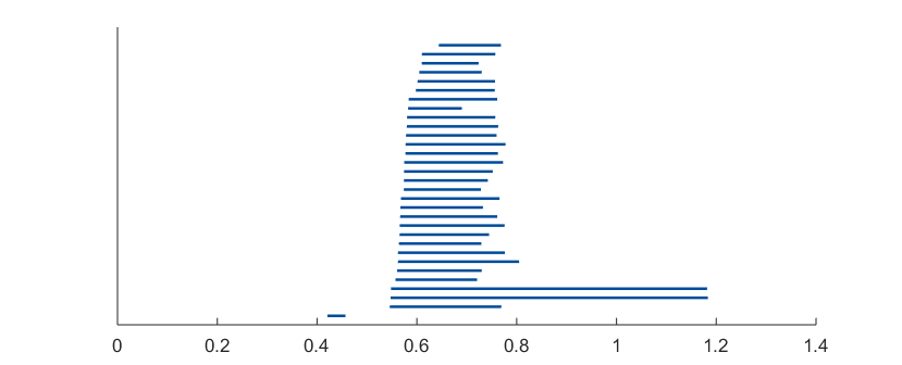
Figure 5. Example of a barcode

Details on the computation of persistent cohomology, and its advantages over persistent homology, can be found in [12].

3. Explicit Classifying Maps

The goal of this section is to derive equation (2), which is in fact a specialization of the proof of Theorem 2.1 to the case of line bundles over metric spaces with finite trivializing covers. When a metric is given, the partition of unity involved in the argument can be described explicitly in terms of bump functions supported on metric balls. Moreover, the local trivializations used in the proof can be replaced by transition functions which — as we will see in sections 4 and 7 — can be calculated in a robust multiscale manner from the persistent cohomology of an appropriate sparse filtration. From this point on, all topological spaces are assumed to be paracompact and Hausdorff.

Classifying maps in terms of local trivializations

Let us sketch the proof of existence in Theorem 2.1 when $B$ has a finite trivializing cover. Starting with local trivializations

(6)

for the vector bundle $\zeta=(E,B,p)$, let $\mu_{r}:p^{-1}(U_{r})\longrightarrow\mathbb{F}^{k}$ be $\mu_{r}\big{(}\rho_{r}(b,\mathbf{v})\big{)}=\mathbf{v}$ for all $(b,\mathbf{v})\in U_{r}\times\mathbb{F}^{k}$.

Definition 3.1.

A collection of continuous maps $\varphi_{r}:U_{r}\longrightarrow\mathbb{R}_{\geq 0}$ is called a partition of unity dominated by $\mathcal{U}=\{U_{r}\}$ if

$$\sum_{r}\varphi_{r}=1\;\;\;\;\;\;\mbox{ and }\;\;\;\;\;\;\mathsf{support}(\varphi_{r})\subset\mathsf{closure}(U_{r})$$

Notice that this notion differs from the usual partition of unity subordinated to a cover in that supports need not be contained in the open sets. However, this is enough for our purposes. Notice that since for paracompact spaces there is always a partition of unity subordinated to a given cover, the same is true in the dominated case.

Let $\psi:[0,1]\longrightarrow[0,1]$ be any homeomorphism so that $\psi(0)=0$ and $\psi(1)=1$. If $\{\varphi_{r}\}$ is a partition of unity dominated by the trivializing cover from equation (6) and we let $\psi_{r}=\psi\circ\varphi_{r}$, then each $\mu_{r}:p^{-1}(U_{r})\longrightarrow\mathbb{F}^{k}$ yields a fiberwise linear map $\widehat{\mu}_{r}:E\longrightarrow\mathbb{F}^{k}$ given by

$$\widehat{\mu}_{r}(e)=\left\{\begin{array}[]{cc}\psi_{r}\big{(}p(e)\big{)}\cdot\mu_{r}(e)&\hbox{ if }\;\;\;p(e)\in U_{r}\\ \\ \mathbf{0}&\hbox{ if }\;\;\;p(e)\notin U_{r}\end{array}\right.$$

Thus one has a continuous map

$$\begin{array}[]{rccc}\widehat{\mu}:&E&\longrightarrow&\mathbb{F}^{k}\oplus\cdots\oplus\mathbb{F}^{k}\\ &e&\mapsto&\left[\widehat{\mu}_{0}(e),\ldots,\widehat{\mu}_{n}(e)\right]\end{array}$$

which, as can be checked, is linear and injective on each fiber. It follows from [27, Lemma 3.1] that the induced continuous map

$$\begin{array}[]{rccc}f_{\zeta}:&B&\longrightarrow&\mathsf{Gr}_{k}\left(\mathbb{F}^{k(n+1)}\right)\\ &b&\mapsto&\widehat{\mu}\left(p^{-1}(b)\right)\end{array}$$

satisfies $f_{\zeta}^{*}\left(\gamma^{k}_{m}\right)\cong\zeta$, if $m=k(n+1)$. This completes the sketch of the proof; let us now describe $f_{\zeta}$ more explicitly in terms of transition functions. The main reason for this change is that transition functions can be determined via a cohomology computation.

Classifying maps from transition functions

Fix $b\in B$ and let $0\leq j\leq n$ be so that $b\in U_{j}$. If $\{\mathbf{v}_{1},\ldots,\mathbf{v}_{k}\}$ is a basis for $\mathbb{F}^{k}$, then $\{\rho_{j}(b,\mathbf{v}_{s})\;|\;s=1,\ldots,k\}$ is a basis for $p^{-1}(b)$ and therefore

$$f_{\zeta}(b)=\mathsf{Span}_{\mathbb{F}}\,\left\{\widehat{\mu}\big{(}\rho_{j}(b,\mathbf{v}_{s})\big{)}\;:\;s=1,\ldots,k\right\}$$ (7)

where

$$\widehat{\mu}\big{(}\rho_{j}(b,\mathbf{v}_{s})\big{)}=\left[\widehat{\mu}_{0}\big{(}\rho_{j}(b,\mathbf{v}_{s})\big{)},\ldots,\widehat{\mu}_{n}\big{(}\rho_{j}(b,\mathbf{v}_{s})\big{)}\right]\in\mathbb{F}^{k(n+1)}$$

If $\{\omega_{rt}:U_{r}\cap U_{t}\longrightarrow\mathsf{GL}_{k}(\mathbb{F})\}$ is the collection of transition functions for $\zeta$ associated to the system of local trivializations $\{\rho_{r}\}$, then whenever $U_{r}\cap U_{t}\neq\emptyset$ we have the commutative diagram

Let $0\leq l\leq n$. If $b\in U_{j}\smallsetminus U_{l}$, then $\widehat{\mu}_{l}\big{(}\rho_{j}(b,\mathbf{v}_{s})\big{)}=0$; else $b\in U_{j}\cap U_{l}$ and

$$\widehat{\mu}_{l}\big{(}\rho_{j}(b,\mathbf{v}_{s})\big{)} = \widehat{\mu}_{l}\left(\rho_{l}\big{(}b,\omega_{jl}(b)^{-1}(\mathbf{v}_{s})\big{)}\right)$$

$$= \psi_{l}(b)\cdot\omega_{lj}(b)(\mathbf{v}_{s})$$

Putting this calculation together with equation (7), it follows that for $b\in U_{j}$

$$f_{\zeta}(b)=\mathsf{Span}_{\mathbb{F}}\Big{\{}\big{[}\psi_{0}(b)\cdot\omega_{0j}(b)(\mathbf{v}_{s})\,,\ldots,\,\psi_{n}(b)\cdot\omega_{nj}(b)(\mathbf{v}_{s})\big{]}\;:\;s=1,\ldots,k\Big{\}}$$ (8)

The case of line bundles

If $k=1$ we can take $\mathbf{v}_{1}=\textbf{1}\in\mathbb{F}$, and abuse notation by writing $\omega_{rt}(b)\in\mathbb{F}^{\times}$ instead of $\omega_{rt}(b)(\mathbf{1})$. Moreover, in this case we have $\mathsf{Gr}_{k}(\mathbb{F}^{k(n+1)})=\mathbb{F}\mathbf{P}^{n}$, and if we use homogeneous coordinates and $\psi(x)=\sqrt{x}$, then $f_{\zeta}:B\longrightarrow\mathbb{F}\mathbf{P}^{n}$ can be expressed locally (i.e. on each $U_{j}$) as

$$f_{\zeta}(b)=\left[\omega_{0j}(b)\cdot\sqrt{\varphi_{0}(b)}:\cdots:\omega_{nj}(b)\cdot\sqrt{\varphi_{n}(b)}\right]\;\;\;\;,\;\;\;\;b\in U_{j}$$

The choice $\psi(x)=\sqrt{x}$ is so that when the transition functions $\omega_{rt}$ are unitary, i.e. $|\omega_{rt}(b)|=1$, then the formula above without homogeneous coordinates produces a representative of $f_{\zeta}(b)$ on the unit sphere of $\mathbb{F}^{n+1}$. We summarize the results thus far in the following theorem:

Theorem 3.2.

Let $B$ be a topological space and let $\mathcal{U}=\{U_{r}\}_{r=0}^{n}$ be an open cover. If $\{\varphi_{r}\}$ is a partition of unity dominated by $\mathcal{U}$, $\mathbb{F}$ is $\mathbb{R}$ or $\mathbb{C}$, and

$$\omega=\big{\{}\omega_{rt}:U_{r}\cap U_{t}\longrightarrow\mathbb{F}^{\times}\big{\}}$$

is a collection of continuous maps satisfying the cocycle condition (4), then the map $f_{\omega}:B\longrightarrow\mathbb{F}\mathbf{P}^{n}$ given in homogenous coordinates by

$$f_{\omega}(b)=\left[\omega_{0j}(b)\cdot\sqrt{\varphi_{0}(b)}:\cdots:\omega_{nj}(b)\cdot\sqrt{\varphi_{n}(b)}\right]\;\;\;\;\;,\;\;\;\;\;b\in U_{j}$$ (9)

is well-defined and classifies the $\mathbb{F}$-line bundle $\zeta_{\omega}$ induced by $(\mathcal{U},\omega)$.

Line bundles over metric spaces

If $B$ comes equipped with a metric $\mathbf{d}$, then (9) can be further specialized to a covering via open balls, and a dominated partition of unity constructed from bump functions supported on the closure of each ball. Indeed, let

$$B_{\epsilon_{r}}(\ell_{r})=\{b\in B\,:\,\mathbf{d}(b,\ell_{r})<\epsilon_{r}\}\;,\;\;\;r=0,\ldots,n$$

for some collection $\{\ell_{0},\ldots,\ell_{n}\}\subset B$ and radii $\epsilon_{r}>0$.

Proposition 3.3.

Let $(B,\mathbf{d})$ be a metric space and let $\mathcal{B}=\{B_{\epsilon_{r}}(\ell_{r})\}_{r=0}^{n}$ be an open cover. If $\phi:\mathbb{R}\longrightarrow\mathbb{R}_{\geq 0}$ is a continuous map so that $\phi^{-1}(0)=\mathbb{R}_{\leq 0}$, and $\lambda_{0},\ldots,\lambda_{n}\in\mathbb{R}_{>0}$ is a set of weights, then

$$\varphi_{r}(b)=\frac{\lambda_{r}\cdot\phi\left(1-\frac{\mathbf{d}(b,\ell_{r})}{\epsilon_{r}}\right)}{\sum\limits_{t=0}^{n}\lambda_{t}\cdot\phi\left(1-\frac{\mathbf{d}(b,\ell_{t})}{\epsilon_{t}}\right)}\;\;,\;\;\;r=0,\ldots,n$$

is a partition of unity for $B$ dominated by $\mathcal{B}$.

Due to the shape of its graph, the map $b\mapsto\lambda_{r}\cdot\phi\left(1-\frac{\mathbf{d}(b,\ell_{r})}{\epsilon_{r}}\right)$ is often referred to as a bump function supported on $\overline{B_{r}}$. The height of the bump is controlled by the weight $\lambda_{r}$, while its overall shape is captured by the function $\phi$. Of course one can choose different functions $\phi_{r}$ on each ball, for instance to capture local density if $B$ comes equipped with a measure. Some examples of bump-shapes are:

• Triangular: The positive part of $x\in\mathbb{R}$ is defined as $\left|x\right|_{+}=\max\{x,0\}$, and $b\mapsto\lambda\cdot\left|1-\frac{\mathbf{d}(b,\ell)}{\epsilon}\right|_{+}$ is the associated triangular bump supported on $\overline{B_{\epsilon}(\ell)}$.

• Polynomial: The polynomial bump with exponent $p>0$ is induced by the function $\phi(x)=\left|x\right|_{+}^{p}$. The triangular bump is recovered when $p=1$, while $p=2$ yields the quadratic bump.

• Gaussian: The Gaussian bump is induced by the funcion

  $$\phi(x)=\left\{\begin{array}[]{cl}e^{-1/x^{2}}&\hbox{if }x>0\\ 0&\hbox{ else}\end{array}\right.$$

• Logarithmic: Is the one associated to $\phi(x)=\log(1+\left|x\right|_{+})$

Figure 6 shows some of these bump functions, with weight $\lambda=1$, for $B_{1}(0)$.

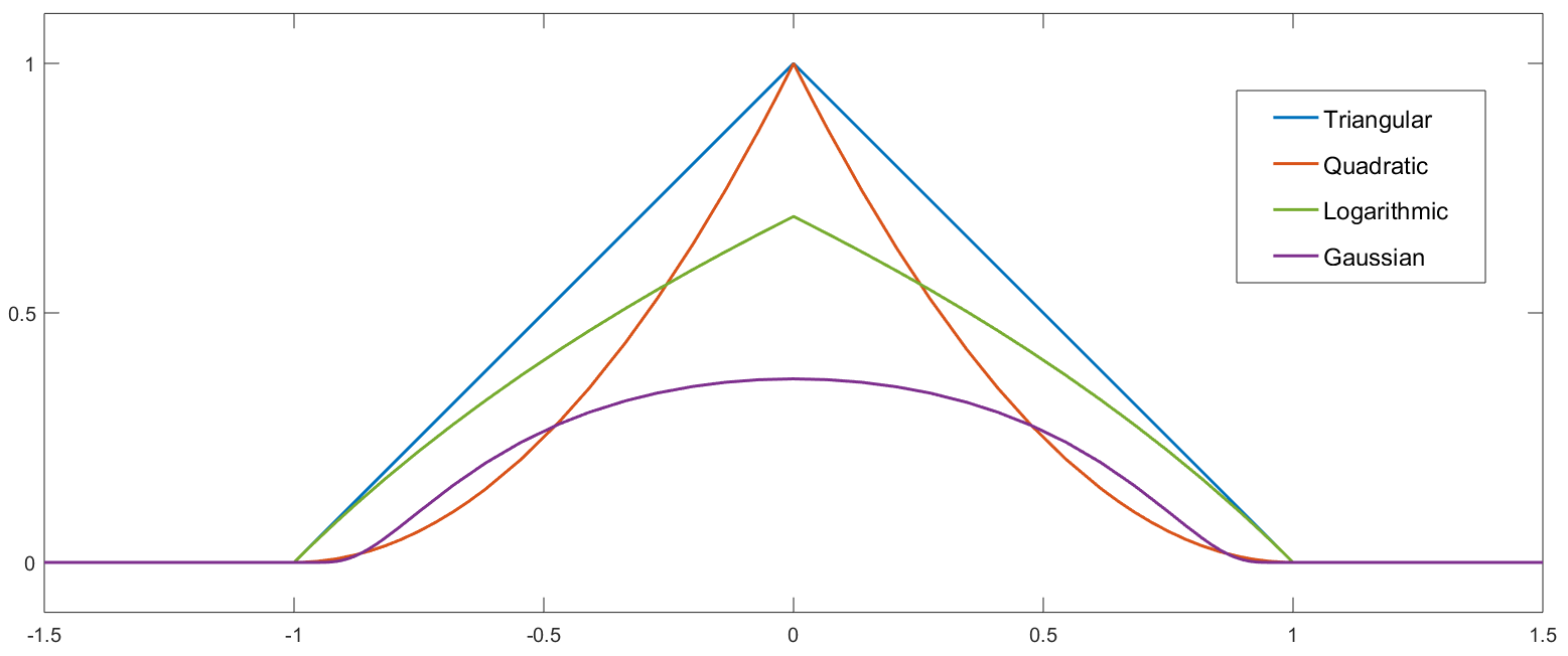
Figure 6. Examples of bump functions supported on $\overline{B_{1}(0)}\subset\mathbb{R}$. Please refer to an online version for colors

Choosing $\phi(x)=\left|x\right|_{+}^{2}$ and the weights as $\lambda_{r}=\epsilon_{r}^{2}$ simplifies Theorem 3.2 to:

Corollary 3.4.

Let $(B,\mathbf{d})$ be a metric space and $\mathcal{B}=\{B_{r}=B_{\epsilon_{r}}(\ell_{r})\}_{r=0}^{n}$ a covering. If $\mathbb{F}$ is $\mathbb{R}$ or $\mathbb{C}$ and $\omega=\{\omega_{rt}:B_{r}\cap B_{t}\longrightarrow\mathbb{F}^{\times}\}$ are continuous maps satisfying the cocycle condition, then $f_{\omega}:B\longrightarrow\mathbb{F}\mathbf{P}^{n}$ given in homogeneous coordinates by

$$f_{\omega}(b)=\Big{[}\omega_{0j}(b)\cdot\left|\epsilon_{0}-\mathbf{d}(b,\ell_{0})\right|_{+}:\cdots:\omega_{nj}(b)\cdot\left|\epsilon_{n}-\mathbf{d}(b,\ell_{n})\right|_{+}\Big{]}\;\;,\;\;\;b\in B_{j}$$

is well-defined and classifies the $\mathbb{F}$-line bundle $\zeta_{\omega}$ induced by $(\mathcal{B},\omega)$.

Geometric Interpretation

Let us clarify (9) for the case of constant transition functions and $\mathbb{F}=\mathbb{R}$. If $\mathcal{U}=\{U_{0},\ldots,U_{n}\}$ is a cover of $B$, then the nerve of $\mathcal{U}$ — denoted $\mathcal{N}(\mathcal{U})$ — is the abstract simplicial complex with one vertex for each open set $U_{r}\in\mathcal{U}$, and a simplex $\{r_{0},\ldots,r_{k}\}$ for each collection $U_{r_{0}},\ldots,U_{r_{k}}\in\mathcal{U}$ such that

$$U_{r_{0}}\cap\cdots\cap U_{r_{k}}\neq\emptyset$$

Given a geometric realization $|\mathcal{N}(\mathcal{U})|\subset\mathbb{R}^{2n+1}$, let $\mathbf{v}_{r}\in|\mathcal{N}(\mathcal{U})|$ be the point corresponding to the vertex $r\in\mathcal{N}(\mathcal{U})$. Each $\mathbf{x}\in|\mathcal{N}(\mathcal{U})|$ is then uniquely determined by (and uniquely determines) its barycentric coordinates: a sequence $\{x_{r}\}$ of real numbers between 0 and 1, one for each open set $U_{r}\in\mathcal{U}$, so that

$$\sum\limits_{r}x_{r}=1\;\;\;\;\mbox{ and }\;\;\;\;\sum_{r}x_{r}\mathbf{v}_{r}=\mathbf{x}$$

To see this, notice that given a non-vertex $\mathbf{x}\in|\mathcal{N}(\mathcal{U})|$ there exists a unique maximal geometric simplex $\sigma$ of $|\mathcal{N}(\mathcal{U})|$ so that $\mathbf{x}$ is in the interior of $\sigma$. If $\mathbf{v}_{r_{0}},\ldots,\mathbf{v}_{r_{k}}\in|\mathcal{N}(\mathcal{U})|$ are the vertices of $\sigma$, then $\mathbf{x}$ can be expressed uniquely as a convex combination of $\mathbf{v}_{r_{0}},\ldots,\mathbf{v}_{r_{k}}$ which determines $x_{r_{0}},\ldots,x_{r_{k}}$. If $r\neq r_{0},\ldots,r_{k}$, then we let $x_{r}=0$.

A partition of unity $\{\varphi_{r}\}$ dominated by $\mathcal{U}$ induces a continuous map

$$\begin{array}[]{rccc}\varphi:&B&\longrightarrow&|\mathcal{N}(\mathcal{U})|\\[2.84544pt] &b&\mapsto&\sum\limits_{r}\varphi_{r}(b)\mathbf{v}_{r}\end{array}$$ (10)

That is, $\varphi$ sends $b$ to the point $\varphi(b)$ with barycentric coordinates $\varphi_{r}(b)$. Moreover, if $\big{\{}\omega_{rt}:U_{r}\cap U_{t}\longrightarrow\{-1,1\}\big{\}}$ is a collection of constant functions satisfying the cocycle condition, then the associated classifying map $f_{\omega}:B\longrightarrow\mathbb{R}\mathbf{P}^{n}$ from Theorem 3.2 can be decomposed as

where $F_{\omega}:|\mathcal{N}(\mathcal{U})|\longrightarrow\mathbb{R}\mathbf{P}^{n}$, in barycentric coordinates, is given on the open star of a vertex $\mathbf{v}_{j}\in|\mathcal{N}(\mathcal{U})|$ as

$$F_{\omega}(x_{0},\ldots,x_{n})=\Big{[}\omega_{0j}\sqrt{x_{0}}:\cdots:\omega_{nj}\sqrt{x_{n}}\Big{]}$$

Example: Let $B=S^{1}$, the unit circle, and let $\mathcal{U}=\{U_{0},U_{1},U_{2}\}$ be the open covering depicted in Figure 7(left).

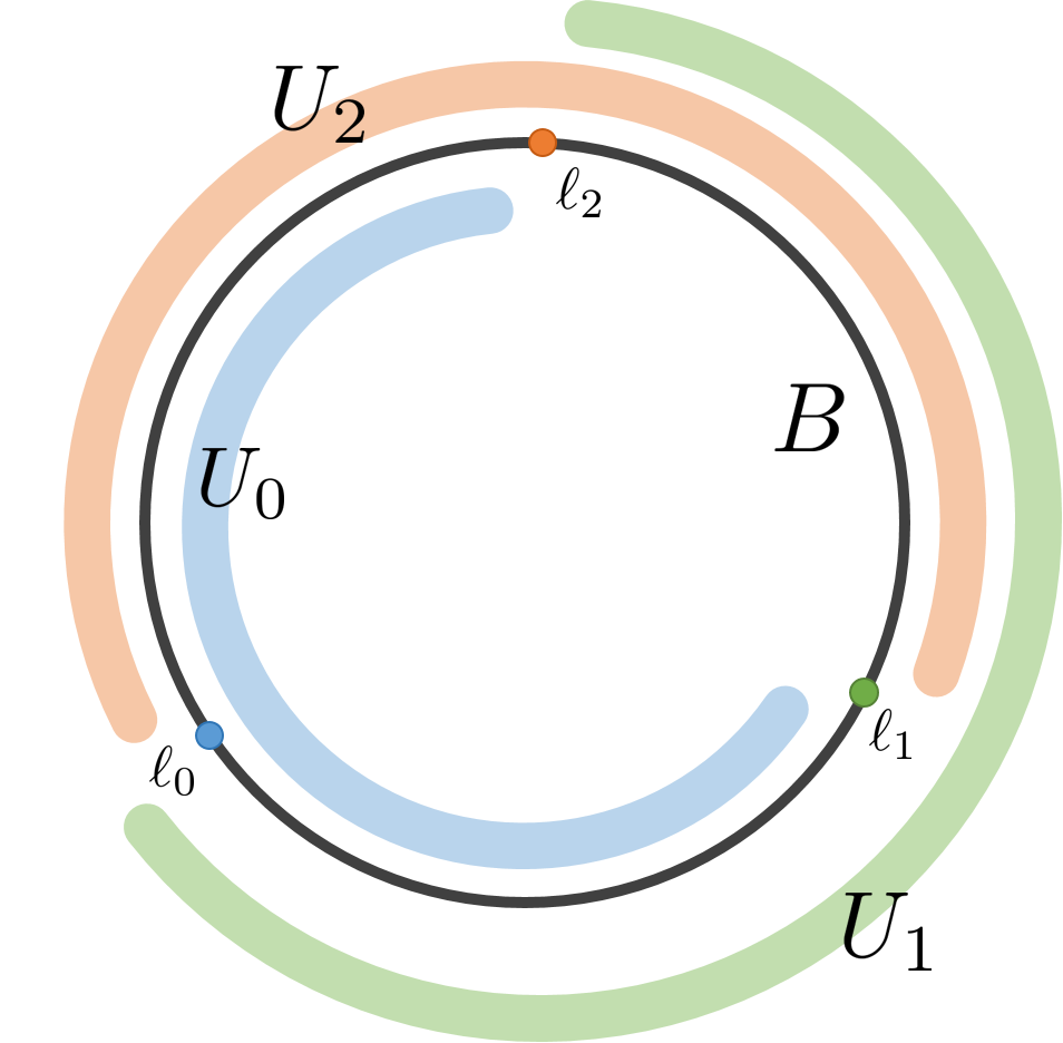
(a) $\mathcal{U}=\{U_{0},U_{1},U_{2}\}$

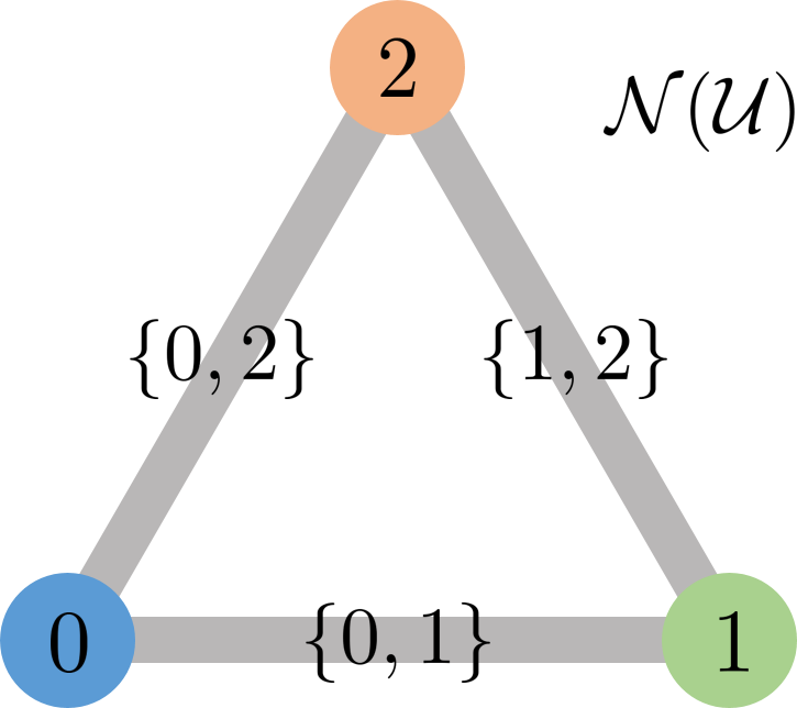
(b) Nerve complex $\mathcal{N}(\mathcal{U})$

Figure 7. An open covering of the circle and the resulting nerve complex.

Define $\omega_{rt}=1$ for $r,t=0,1,2$; let $\omega^{\prime}_{02}=\omega^{\prime}_{20}=-1$ and let $\omega^{\prime}_{rt}=1$ for all $(r,t)\neq(0,2),(2,0)$. Let $(x_{0},x_{1},x_{2})$ denote the barycentric coordinates of a point in $|\mathcal{N}(\mathcal{U})|$. For instance, the vertex labeled as $0$ has coordinates $(1,0,0)$ and the midpoint of the edge $\{0,1\}$ has coordinates $(1/2,1/2,0)$. Then

$$F_{\omega}(x_{0},x_{1},x_{2})=\big{[}\sqrt{x_{0}}:\sqrt{x_{1}}:\sqrt{x_{2}}\big{]}$$

and for each $0\leq x\leq 1$

$$F_{\omega^{\prime}}(x,1-x,0) = \Big{[}\sqrt{x}:\sqrt{1-x}:0\Big{]}$$

$$F_{\omega^{\prime}}(x,0,1-x) = \Big{[}\sqrt{x}:0:-\sqrt{1-x}\Big{]}$$

$$F_{\omega^{\prime}}(0,x,1-x) = \Big{[}0:\sqrt{x}:\sqrt{1-x}\Big{]}$$

We show in Figure 8 how $F_{\omega}$ and $F_{\omega^{\prime}}$ map $|\mathcal{N}(\mathcal{U})|$ to $\mathbb{R}\mathbf{P}^{2}=S^{2}/(\mathbf{x}\sim-\mathbf{x})$.

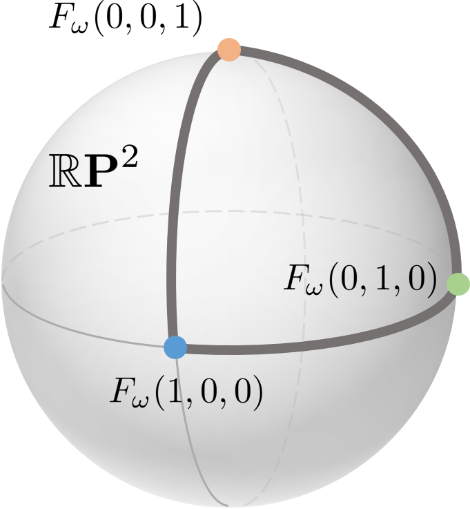
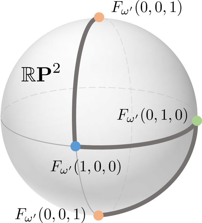
Figure 8. Image of $F_{\omega}$ (left) and $F_{\omega^{\prime}}$ (right) in $\mathbb{R}\mathbf{P}^{2}=S^{2}/(\mathbf{u}\sim-\mathbf{u})$.

If $\mathbf{d}$ is the geodesic distance on $S^{1}$, then each arc $U_{r}$ is an open ball $B_{\epsilon_{r}}(\ell_{r})$ for some $(\epsilon_{r},\ell_{r})\in\mathbb{R}^{+}\times S^{1}$. When $\varphi:S^{1}\longrightarrow|\mathcal{N}(\mathcal{U})|$ is induced by the partition of unity from the triangular bumps $\phi(x)=\left|x\right|_{+}$, then $\varphi$ maps each arc $\{\ell_{r},\ell_{t}\}$ linearly onto the edge $|\{r,t\}|$. It is not hard to see that the $\mathbb{R}$-line bundle induced by $\{\omega_{rt}\}$ is trivial, while the one induced by $\{\omega^{\prime}_{rt}\}$ is the nontrivial bundle on $S^{1}$ having the Moebius band as total space. This is captured by $f_{\omega}=F_{\omega}\circ\varphi:S^{1}\longrightarrow\mathbb{R}\mathbf{P}^{2}$ being null-homotopic and $f_{\omega^{\prime}}=F_{\omega^{\prime}}\circ\varphi$ representing the nontrivial element in the fundamental group $\pi_{1}(\mathbb{R}\mathbf{P}^{2})\cong\mathbb{Z}/2$.

4. Transition Functions from Simplicial Cohomology

Let $\mathcal{U}=\{U_{r}\}$ be a cover for $B$. We have shown thus far that given a collection $\omega=\{\omega_{rt}\}$ of continuous maps

$$\omega_{rt}:U_{r}\cap U_{t}\longrightarrow\mathsf{GL}_{1}(\mathbb{F})=\mathbb{F}^{\times}\;,\;\;U_{r}\cap U_{t}\neq\emptyset$$

satisfying the cocycle condition, one can explicitly write down (given a dominated partition of unity) a classifying map $f_{\omega}:B\longrightarrow\mathbb{F}\mathbf{P}^{n}$ for the associated $\mathbb{F}$-line bundle $\zeta_{\omega}$. What we will see next is that determining such transition functions can be reduced to a computation in simplicial cohomology.

Formulation in Terms of Sheaf Cohomology

If $\mathscr{C}_{\mathbb{F}}^{\times}$ denotes the sheaf of continuous $\mathbb{F}^{\times}$-valued functions on $B$, then one has that $\omega\in\check{C}^{1}(\mathcal{U};\mathscr{C}_{\mathbb{F}}^{\times})$. Moreover, since $\omega$ satisfies the cocycle condition, then $\omega\in\check{Z}^{1}(\mathcal{U};\mathscr{C}_{\mathbb{F}}^{\times})$, and hence we can consider the cohomology class $[\omega]\in\check{H}^{1}(\mathcal{U};\mathscr{C}_{\mathbb{F}}^{\times})$. If $\mathcal{V}$ is another covering of $B$ we say that $\mathcal{V}$ is a refinement of $\mathcal{U}$, denoted $\mathcal{V}\prec\mathcal{U}$, if for every $V\in\mathcal{V}$ there exists $U\in\mathcal{U}$ so that $V\subset U$. A standard result (Exercise 6.2, [1]) is the following:

Lemma 4.1.

If $\omega,\omega^{\prime}\in\check{Z}^{1}(\mathcal{U};\mathscr{C}_{\mathbb{F}}^{\times})$ are cohomologous, then $\zeta_{\omega}\cong\zeta_{\omega^{\prime}}$. Moreover, the function

$$\begin{array}[]{ccc}\check{H}^{1}(\mathcal{U};\mathscr{C}_{\mathbb{F}}^{\times})&\longrightarrow&\mathsf{Vec}^{1}_{\mathbb{F}}(B)\\[2.84544pt] [\,\omega\,]&\mapsto&[\,\zeta_{\omega}\,]\end{array}$$

is an injective homomorphism, and natural with respect to refinements of $\mathcal{U}$.

Here natural means that if $H^{\mathcal{U}}_{\mathcal{V}}:\check{H}^{1}(\mathcal{U};\mathscr{C}_{\mathbb{F}}^{\times})\longrightarrow\check{H}^{1}(\mathcal{V};\mathscr{C}_{\mathbb{F}}^{\times})$ is the homomorphism induced by the refinement $\mathcal{V}\prec\mathcal{U}$ (see [28, Chapter IX, Lemma 3.10]), then the diagram

is commutative. Combining this with equation (3) yields

Corollary 4.2.

Let $\mathcal{U}$ be an open covering of $B$. Then the function

$$\begin{array}[]{rccc}\Gamma_{\mathcal{U}}:&\check{H}^{1}(\mathcal{U};\mathscr{C}_{\mathbb{F}}^{\times})&\longrightarrow&\big{[}B\,,\,\mathbb{F}\mathbf{P}^{\infty}\big{]}\\[2.84544pt] &[\omega]&\mapsto&[f_{\omega}]\end{array}$$

is injective, and natural with respect to refinements of $\mathcal{U}$.

The sheaf cohomology group $\check{H}^{1}(\mathcal{U};\mathscr{C}_{\mathbb{F}}^{\times})$ can be replaced, under suitable conditions, by simplicial cohomology groups: $H^{1}(\mathcal{N}(\mathcal{U});\mathbb{Z}/2)$ when $\mathbb{F}=\mathbb{R}$, and $H^{2}(\mathcal{N}(\mathcal{U});\mathbb{Z})$ when $\mathbb{F}=\mathbb{C}$. We will not assume that $\mathcal{U}$ is a good cover (i.e. that each finite intersection $U_{r_{0}}\cap\ldots\cap U_{r_{k}}$ is either empty or contractible), but rather will phrase the reduction theorems in terms of the relevant connectivity conditions. The construction is described next.

Reduction to Simplicial Cohomology

If $\tau\in Z^{1}(\mathcal{N}(\mathcal{U});\mathbb{Z}/2)$, then for each $U_{r}\cap U_{t}\neq\emptyset$ we have $\tau(\{r,t\})=\tau_{rt}\in\{0,1\}=\mathbb{Z}/2$. Let $\phi^{\tau}=\{\phi^{\tau}_{rt}\}$ be the collection of constant functions

$$\begin{array}[]{rccc}\phi_{rt}^{\tau}:&U_{r}\cap U_{t}&\longrightarrow&\mathbb{R}^{\times}\\ &y&\mapsto&(-1)^{\tau_{rt}}\end{array}$$

Therefore each $\phi^{\tau}_{rt}$ is continuous, so $\phi^{\tau}\in\check{C}^{1}(\mathcal{U};\mathscr{C}_{\mathbb{R}}^{\times})$, and since $\tau$ is a cocycle it follows that $\phi^{\tau}\in\check{Z}^{1}(\mathcal{U};\mathscr{C}_{\mathbb{R}}^{\times})$. Moreover, the association $\tau\mapsto\phi^{\tau}$ induces the homomorphism

$$\begin{array}[]{rccc}\Phi_{\mathcal{U}}:&H^{1}(\mathcal{N}(\mathcal{U});\mathbb{Z}/2)&\longrightarrow&\check{H}^{1}(\mathcal{U};\mathscr{C}_{\mathbb{R}}^{\times})\\ &[\tau]&\mapsto&\left[\phi^{\tau}\right]\end{array}$$

which is well-defined and satisfies:

Proposition 4.3.

$$\Phi_{\mathcal{U}}:H^{1}(\mathcal{N}(\mathcal{U});\mathbb{Z}/2)\longrightarrow\check{H}^{1}(\mathcal{U};\mathscr{C}^{\times}_{\mathbb{R}})$$

is natural with respect to refinements. Moreover, if each $U_{r}$ is connected, then $\Phi_{\mathcal{U}}$ is injective.

Proof.

Fix $\tau\in Z^{1}(\mathcal{N}(\mathcal{U});\mathbb{Z}/2)$ and assume that there is a collection of continuous maps $\{f_{r}:U_{r}\longrightarrow\mathbb{R}^{\times}\}$ for which $(-1)^{\tau_{rt}}=\frac{f_{t}}{f_{r}}$ on $U_{r}\cap U_{t}\neq\emptyset$. If each element of $\mathcal{U}$ is connected, then the $f_{r}$’s have constat sign (either $+1$ or $-1$) in their domains, and hence we can define $\nu\in C^{0}(\mathcal{N}(\mathcal{U});\mathbb{Z}/2)$ as

$$\nu(\{r\})=\frac{1-\mathsf{sign}(f_{r})}{2}$$

Therefore $\tau(\{r,t\})=\delta^{0}(\nu)(\{r,t\})$ and the result follows. ∎

Define $\mathbf{w}_{1}^{\mathcal{U}}$ as the composition

Corollary 4.4.

If each $U_{r}$ is connected, then

$$\mathbf{w}_{1}^{\mathcal{U}}:H^{1}(\mathcal{N}(\mathcal{U});\mathbb{Z}/2)\longrightarrow[B\,,\,\mathbb{R}\mathbf{P}^{\infty}]$$

is injective and natural with respect to refinements.

Let us now address the complex case. Given $\sigma\in Z^{2}(\mathcal{N}(\mathcal{U});\mathbb{Z})$ let $\psi^{\sigma}=\{\psi^{\sigma}_{rst}\}$ be the collection of constant functions

$$\begin{array}[]{rccc}\psi^{\sigma}_{rst}:&U_{r}\cap U_{s}\cap U_{t}&\longrightarrow&\mathbb{Z}\\ &y&\mapsto&\sigma_{rst}\end{array}$$

Each $\psi_{rst}^{\sigma}$ is locally constant and therefore $\psi^{\sigma}\in\check{Z}^{2}(\mathcal{U};\underline{\mathbb{Z}})$. It follows that the association $\sigma\mapsto\psi^{\sigma}$ induces a homomorphism

$$\begin{array}[]{rccc}\Psi_{\mathcal{U}}:&H^{2}(\mathcal{N}(\mathcal{U});\mathbb{Z})&\longrightarrow&\check{H}^{2}(\mathcal{U};\underline{\mathbb{Z}})\\ &[\sigma]&\mapsto&\left[\psi^{\sigma}\right]\end{array}$$

which is well-defined and satisfies:

Proposition 4.5.

$$\Psi_{\mathcal{U}}:H^{2}(\mathcal{N}(\mathcal{U});\mathbb{Z})\longrightarrow\check{H}^{2}(\mathcal{U};\underline{\mathbb{Z}})$$

is natural with respect to refinements. Moreover, if each $U_{r}\cap U_{t}$ is either empty or connected, then $\Psi_{\mathcal{U}}$ is injective.

Proof.

The result is deduced from the following observation: if $U_{r}\cap U_{t}$ is connected, then any function $\mu_{rt}:U_{r}\cap U_{t}\longrightarrow\mathbb{Z}$ which is locally constant is in fact constant. ∎

We will now link $\check{H}^{2}(\mathcal{U};\underline{\mathbb{Z}})$ and $\check{H}^{1}(\mathcal{U};\mathscr{C}_{\mathbb{C}}^{\times})$ using the exponential sequence

which is given at the level of open sets $U\in\mathcal{U}$ by

If $\mathfrak{Im}(\exp)$ denotes the image presheaf

$$\mathfrak{Im}(\exp)\big{(}U\big{)}=Img\left\{\leavevmode\hbox to89.15pt{\vbox to18.39pt{\text{[drawing]}}}\right\} {\mathscr{C}_{\mathbb{C}}(U)} {\mathscr{C}_{\mathbb{C}}^{\times}(U)} \scriptstyle{\exp} {\mathscr{C}_{\mathbb{C}}(U)} {\mathscr{C}_{\mathbb{C}}^{\times}(U)} \scriptstyle{\exp}$$

then

is a short exact sequence of presheaves (i.e. exact for every open set), and hence we get a long exact sequence in Čech cohomology [35, Section 24]

Since $\mathscr{C}_{\mathbb{C}}$ admits partitions of unity (i.e. it is a fine sheaf), then

Lemma 4.6.

$\check{H}^{k}(\mathcal{U};\mathscr{C}_{\mathbb{C}})=0$ for every $k\geq 1$.

Hence $\Delta:\check{H}^{1}(\mathcal{U};\mathfrak{Im}(\exp))\longrightarrow\check{H}^{2}(\mathcal{U};\underline{\mathbb{Z}})$ is an isomorphism. Moreover,

Proposition 4.7.

Let $\{\varphi_{t}\}$ be a continuous partition of unity dominated by $\mathcal{U}$. If $\eta=\{\eta_{rst}\}\in Z^{2}(\mathcal{N}(\mathcal{U});\mathbb{Z})$, then

$$\omega_{rs}=\exp\Big{(}2\pi i\sum_{t}\varphi_{t}\cdot\eta_{rst}\Big{)}\;\;,\;\;\;U_{r}\cap U_{s}\neq\emptyset$$

defines an element $\omega=\{\omega_{rs}\}\in\check{C}^{1}(\mathcal{U};\mathfrak{Im}(\exp))$. Moreover, $\omega$ is a Čech cocycle, and the composition

satisfies $\Delta^{-1}\circ\Psi_{\mathcal{U}}\big{(}[\eta]\big{)}=[\omega]$.

Proof.

First we check that $\omega$ is a Čech cocycle:

$$\omega_{rs}\cdot\omega_{st} = \exp\left(2\pi i\sum_{\ell}\varphi_{\ell}\cdot(\eta_{rs\ell}+\eta_{st\ell})\right)$$

$$= \exp\left(2\pi i\sum_{\ell}\varphi_{\ell}\cdot(\eta_{rt\ell}+\eta_{rst})\right)$$

$$= \exp\left(2\pi i\cdot\eta_{rst}+\sum_{\ell}\varphi_{\ell}\cdot\eta_{rt\ell}\right)$$

$$= \omega_{rt}$$

In order to see that $\Delta([\omega])=\Psi_{\mathcal{U}}([\eta])$, we use the definition of the connecting homomorphism $\Delta$. First, we let $g=\{g_{rs}\}\in\check{C}^{1}(\mathcal{U};\mathscr{C}_{\mathbb{C}})$ be the collection of functions

$$g_{rs}(b)=\sum_{\ell}\varphi_{\ell}(b)\cdot\eta_{rs\ell}\;\;\;\;\;\;\;b\in U_{r}\cap U_{s}$$

It follows that $\omega=\exp^{\#}(g)$ and therefore $\Delta([\omega])=[\delta^{1}(g)]$. The coboundary $\delta^{1}(g)$ can be computed as

$$\delta^{1}(g)_{rst} = g_{rs}-g_{rt}+g_{st}$$

$$= \sum_{\ell}\varphi_{\ell}\cdot(\eta_{rs\ell}-\eta_{rt\ell}+\eta_{st\ell})$$

$$= \sum_{\ell}\varphi_{\ell}\cdot\eta_{rst}$$

$$= \eta_{rst}$$

and therefore $\Delta([\omega])=\Psi_{\mathcal{U}}([\eta]).$ ∎

Corollary 4.8.

If each $U_{r}\cap U_{t}$ is either empty or connected, then

$$\begin{array}[]{cccc}\Delta^{-1}\circ\Psi_{\mathcal{U}}:&H^{2}(\mathcal{N}(\mathcal{U});\mathbb{Z})&\longrightarrow&\check{H}^{1}(\mathcal{U};\mathfrak{Im}(\exp))\\ &[\{\eta_{rst}\}]&\mapsto&[\{\omega_{rs}\}]\end{array}$$

is injective, where $\omega_{rs}=\exp\Big{(}2\pi i\sum\limits_{t}\varphi_{t}\cdot\eta_{rst}\Big{)}$.

When going from $\check{H}^{1}(\mathcal{U};\mathfrak{Im}(\exp))$ to $\check{H}^{1}(\mathcal{U};\mathscr{C}_{\mathbb{C}}^{\times})$ one considers the inclusion of presheaves $\jmath:\mathfrak{Im}(\exp)\longrightarrow\mathscr{C}_{\mathbb{C}}^{\times}$ and its induced homomorphism in cohomology

$$\jmath_{\mathcal{U}}:\check{H}^{1}(\mathcal{U};\mathfrak{Im}(\exp))\longrightarrow\check{H}^{1}(\mathcal{U};\mathscr{C}_{\mathbb{C}}^{\times})$$

After taking direct limits over refinements of $\mathcal{U}$, the resulting homomorphism is an isomorphism [35, Proposition 7, section 25]. That is, each element in $\ker(\jmath_{\mathcal{U}})$ is also in the kernel of $\check{H}^{1}(\mathcal{U};\mathfrak{Im}(\exp))\longrightarrow\check{H}^{1}(\mathcal{V};\mathfrak{Im}(\exp))$ for some refinement $\mathcal{V}$ of $\mathcal{U}$; and for every element in $\check{H}^{1}(\mathcal{U};\mathscr{C}_{\mathbb{C}}^{\times})$ there exists a refinement $\mathcal{W}$ of $\mathcal{U}$ so that the image of said element via $\check{H}^{1}(\mathcal{U};\mathscr{C}_{\mathbb{C}}^{\times})\longrightarrow\check{H}^{1}(\mathcal{W};\mathscr{C}_{\mathbb{C}}^{\times})$ is also in the image of $\check{H}^{1}(\mathcal{W};\mathfrak{Im}(\exp))\longrightarrow\check{H}^{1}(\mathcal{W};\mathscr{C}_{\mathbb{C}}^{\times})$.

The situation is sometimes simpler. Recall that a topological space is said to be simply connected if it is path-connected and its fundamental group is trivial. In addition, it is said to be locally path-connected if each point has a path-connected open neighborhood.

Lemma 4.9.

Let $\mathcal{U}=\{U_{r}\}$ be an open covering of $B$ such that each $U_{r}$ is locally path-connected and simply connected. Then

$$\jmath_{\mathcal{U}}:\check{H}^{1}(\mathcal{U};\mathfrak{Im}(\exp))\longrightarrow\check{H}^{1}(\mathcal{U};\mathscr{C}^{\times}_{\mathbb{C}})$$

is injective.

Proof.

Let $[\{\omega_{rt}\}]\in\check{H}^{1}(\mathcal{U};\mathfrak{Im}(\exp))$ be an element in the kernel of $\jmath_{\mathcal{U}}$. Then there exists a collection of continuous maps

$$\nu_{r}:U_{r}\longrightarrow\mathbb{C}^{\times}$$

so that $\omega_{rt}=\frac{\nu_{t}}{\nu_{r}}$ on $U_{r}\cap U_{t}\neq\emptyset$. If we let

$$\begin{array}[]{rccl}p:&\mathbb{R}_{+}\times\mathbb{R}&\longrightarrow&\mathbb{C}^{\times}\\ &(\rho,\theta)&\mapsto&\rho\cdot e^{2\pi i\cdot\theta}\end{array}$$

then it follows that $\left(\mathbb{R}_{+}\times\mathbb{R}\,,\,p\right)$ is the universal cover for $\mathbb{C}^{\times}$. Moreover, since each $U_{r}$ is locally path-connected and simply connected, then each $\nu_{r}$ has a lift [19, Proposition 1.33]

$$\begin{array}[]{rccl}\widetilde{\nu}_{r}:&U_{r}&\longrightarrow&\mathbb{R}_{+}\times\mathbb{R}\\ &b&\mapsto&\big{(}\rho_{r}(b),\theta_{r}(b)\big{)}\end{array}$$

That is $p\circ\widetilde{\nu}_{r}(b)=\nu_{r}(b)$ for all $b\in U_{r}$. Let $\phi_{r}:U_{r}\longrightarrow\mathbb{C}$ be defined as

$$\phi_{r}(b)=\theta_{r}(b)-i\frac{\ln(\rho_{r}(b))}{2\pi}$$

It follows that $\{\phi_{r}\}\in\check{C}^{0}(\mathcal{U};\mathscr{C}_{\mathbb{C}})$ and that for all $b\in U_{r}$

$$\exp\big{(}2\pi i\cdot\phi_{r}(b)\big{)} = \exp\big{(}\ln(\rho_{r}(b))+2\pi i\cdot\theta_{r}(b)\big{)}$$

$$= \rho_{r}(b)\cdot e^{2\pi i\cdot\theta_{r}(b)}$$

$$= \nu_{r}(b)$$

Therefore $\nu_{r}=\exp(2\pi i\cdot\phi_{r})$ and $\{\nu_{r}\}\in\check{C}^{0}(\mathcal{U};\mathfrak{Im}(\exp))$, which implies $[\{\omega_{rt}\}]=0$ in $\check{H}^{1}(\mathcal{U};\mathfrak{Im}(\exp))$ as claimed. ∎

In summary, given an open cover $\mathcal{U}$ of $B$ we get the function

which is natural with respect to refinements and satisfies:

Corollary 4.10.

Let $\mathcal{U}=\{U_{j}\}$ be an open cover of $B$ such that each $U_{r}$ is locally path-connected and simply connected, and each $U_{r}\cap U_{t}$ is either empty or connected. Then

$$\mathbf{c}_{1}^{\mathcal{U}}:H^{2}(\mathcal{N}(\mathcal{U});\mathbb{Z})\longrightarrow\big{[}B\,,\,\mathbb{C}\mathbf{P}^{\infty}\big{]}$$

is injective.

We summarize the results of this section in the following theorem:

Theorem 4.11.

Let $\mathcal{U}=\{U_{0},\ldots,U_{n}\}$ be an open cover of $B$, and let $\{\varphi_{r}\}$ be a partition of unity dominated by $\mathcal{U}$. Then we have functions

$$\begin{array}[]{rccc}\mathbf{w}^{\mathcal{U}}_{1}:&H^{1}(\mathcal{N}(\mathcal{U});\mathbb{Z}/2)&\longrightarrow&\big{[}B\,,\,\mathbb{R}\mathbf{P}^{\infty}\big{]}\\[2.84544pt] &[\tau=\{\tau_{rt}\}]&\mapsto&[f_{\tau}]\end{array}\mbox{ , }\begin{array}[]{rccc}\mathbf{c}^{\mathcal{U}}_{1}:&H^{2}(\mathcal{N}(\mathcal{U});\mathbb{Z})&\longrightarrow&\big{[}B\,,\,\mathbb{C}\mathbf{P}^{\infty}\big{]}\\[2.84544pt] &[\eta=\{\eta_{rst}\}]&\mapsto&[f_{\eta}]\end{array}$$

natural w.r.t refinements of $\mathcal{U}$, where $\tau_{rt}=\tau(\{r,t\})$, $\eta_{rst}=\eta(\{r,s,t\})$ and

$$\begin{array}[]{rccl}f_{\tau}:&B&\longrightarrow&\mathbb{R}\mathbf{P}^{n}\\ &U_{j}\ni b&\mapsto&\left[(-1)^{\tau_{0j}}\sqrt{\varphi_{0}(b)}:\cdots:(-1)^{\tau_{nj}}\sqrt{\varphi_{n}(b)}\right]\\ \\ f_{\eta}:&B&\longrightarrow&\mathbb{C}\mathbf{P}^{n}\\ &U_{j}\ni b&\mapsto&\left[e^{2\pi i\sum\limits_{t}\varphi_{t}(b)\eta_{0jt}}\sqrt{\varphi_{0}(b)}\;:\cdots:\;e^{2\pi i\sum\limits_{t}\varphi_{t}(b)\eta_{njt}}\sqrt{\varphi_{n}(b)}\right]\end{array}$$

are well-defined. Moreover, if each $U_{r}$ is connected, then $\mathbf{w}_{1}^{\mathcal{U}}$ is injective; if in addition each $U_{r}$ is locally path-connected and simply connected, and each $U_{r}\cap U_{t}$ is either empty or connected, then $\mathbf{c}_{1}^{\mathcal{U}}$ is injective.

5. Dimensionality Reduction in $\mathbb{F}\mathbf{P}^{n}$ via Principal Projective Coordinates

Let $V\subset\mathbb{F}^{n+1}$ be a linear subspace with $\dim(V)\geq 1$. If $\sim$ is the equivalence relation on $\mathbb{F}^{n+1}\smallsetminus\{\mathbf{0}\}$ given by $\mathbf{u}\sim\mathbf{v}$ if and only if $\mathbf{u}=\lambda\mathbf{v}$ for some $\lambda\in\mathbb{F}$, then $\sim$ is also an equivalence relation on $V\smallsetminus\{\mathbf{0}\}$ and hence we can define

$$\mathbb{F}\mathbf{P}^{\dim(V)-1}_{V}:=\big{(}V\smallsetminus\{\mathbf{0}\}\big{)}\big{/}\sim$$

In particular $\mathbb{F}\mathbf{P}^{\dim(U)-1}_{U}=\mathbb{F}\mathbf{P}^{\dim(V)-1}_{V}$ if and only if $U=V$, and $\mathbb{F}\mathbf{P}_{V}^{\dim(V)-1}$ is a subset of $\mathbb{F}\mathbf{P}^{n}$. Recall that $\mathbb{F}$ is either $\mathbb{R}$ or $\mathbb{C}$. For $\mathbf{u},\mathbf{v}\in\mathbb{F}^{n+1}$ let

$$\langle\mathbf{u},\mathbf{v}\rangle=\sum_{r=0}^{n}u_{r}\cdot\overline{v}_{r}$$

denote their inner product. If $\mathbf{d}_{g}$ denotes the geodesic distance in $\mathbb{F}\mathbf{P}^{n}$ induced by the Fubini-Study metric, then one has that

$$\mathbf{d}_{g}([\mathbf{u}],[\mathbf{v}])=\arccos\left(\frac{|\langle\mathbf{u},\mathbf{v}\rangle|}{\|\mathbf{u}\|\cdot\|\mathbf{v}\|}\right)$$

and it can be checked that $\mathbb{F}\mathbf{P}^{\dim(V)-1}_{V}$ is an isometric copy of $\mathbb{F}\mathbf{P}^{\dim(V)-1}$ inside $\mathbb{F}\mathbf{P}^{n}$.

If $1\leq\dim(V)\leq n$ and $V^{\perp}=\{\mathbf{u}\in\mathbb{F}^{n+1}:\langle\mathbf{u},\mathbf{v}\rangle=0\mbox{ for all }\mathbf{v}\in V\}$, then the orthogonal projection $p_{V}:\mathbb{F}^{n+1}\longrightarrow V$ descends to a continuous map

$$\begin{array}[]{rrcl}P_{V}:&\mathbb{F}\mathbf{P}^{n}\smallsetminus\mathbb{F}\mathbf{P}_{V^{\perp}}^{n-\dim(V)}&\longrightarrow&\mathbb{F}\mathbf{P}_{V}^{\dim(V)-1}\\ &\,[\mathbf{u}]&\mapsto&[\,p_{V}(\mathbf{u})]\end{array}$$

Recall that $p_{V}$ sends each $\mathbf{u}\in\mathbb{F}^{n+1}$ to its closest point in $V$ with respect to the distance induced by $\|\cdot\|$. A similar property is inherited by $P_{V}$:

Proposition 5.1.

If $[\mathbf{w}]\in\mathbb{F}\mathbf{P}^{n}\smallsetminus\mathbb{F}\mathbf{P}_{V^{\perp}}^{n-\dim(V)}$, then $P_{V}([\mathbf{w}])$ is the point in $\mathbb{F}\mathbf{P}_{V}^{\dim(V)-1}$ which is closest to $[\mathbf{w}]$ with respect to $\mathbf{d}_{g}$.

Proof.

Let $[\mathbf{u}]\in\mathbb{F}\mathbf{P}^{\dim(V)-1}_{V}$. Since $[\mathbf{w}]\notin\mathbb{F}\mathbf{P}_{V^{\perp}}^{n-\dim(V)}$, then $\mathbf{w}-p_{V}(\mathbf{w})\in V^{\perp}$ with $p_{V}(\mathbf{w})\neq\mathbf{0}$. Therefore $\langle\mathbf{u},\mathbf{w}-p_{U}(\mathbf{w})\rangle=0$ and by the Cauchy-Schwartz inequality

$$\left|\left\langle\mathbf{w},\mathbf{u}\right\rangle\right|=|\langle p_{U}(\mathbf{w}),\mathbf{u}\rangle|\leq\|p_{U}(\mathbf{w})\|\cdot\|\mathbf{u}\|$$

Hence

$$\frac{|\langle\mathbf{w},\mathbf{u}\rangle|}{\|\mathbf{w}\|\cdot\|\mathbf{u}\|}\leq\frac{\|p_{U}(\mathbf{w})\|}{\|\mathbf{w}\|}=\frac{|\langle\mathbf{w},p_{U}(\mathbf{w})\rangle|}{\|\mathbf{w}\|\cdot\|p_{U}(\mathbf{w})\|}$$

and since $\arccos(\alpha)$ is decreasing, then $\mathbf{d}_{g}([\mathbf{w}],P_{U}([\mathbf{w}]))\leq\mathbf{d}_{g}([\mathbf{w}],[\mathbf{u}])$. ∎

Therefore, we can think of $P_{V}$ as the projection onto $\mathbb{F}\mathbf{P}_{V}^{\dim(V)-1}$. Moreover, let $\jmath_{V}:\mathbb{F}\mathbf{P}_{V}^{\dim(V)-1}\hookrightarrow\mathbb{F}\mathbf{P}^{n}\smallsetminus\mathbb{F}\mathbf{P}^{n-\dim(V)}_{V^{\perp}}$ be the inclusion map.

Proposition 5.2.

$\jmath_{V}\circ P_{V}$ is a deformation retraction.

Proof.

Since $p_{V}$ is surjective and satisfies $p_{V}\circ p_{V}(\mathbf{w})=p_{V}(\mathbf{w})$ for all $\mathbf{w}\in\mathbb{F}^{n+1}$, it follows that $P_{V}$ is a retraction. Let $h:\mathbb{F}^{n+1}\times[0,1]\longrightarrow\mathbb{F}^{n+1}$ be given by $h(\mathbf{w},t)=(1-t)\cdot\mathbf{w}+t\cdot p_{V}(\mathbf{w})$. Since $h(\mathbf{w},t)=\mathbf{0}$ implies that $\mathbf{w}\in V^{\perp}$, then $h$ induces a continuous map

$$\begin{array}[]{rcl}\left(\mathbb{F}\mathbf{P}^{n}\smallsetminus\mathbb{F}\mathbf{P}_{V^{\perp}}^{n-\dim(V)}\right)\times[0,1]&\longrightarrow&\mathbb{F}\mathbf{P}^{n}\smallsetminus\mathbb{F}\mathbf{P}_{V^{\perp}}^{n-\dim(V)}\\[2.84544pt] \big{(}[\mathbf{w}],t\big{)}&\mapsto&[h(\mathbf{w},t)]\end{array}$$

which is a homotopy between the identity of $\mathbb{F}\mathbf{P}^{n}\smallsetminus\mathbb{F}\mathbf{P}_{V^{\perp}}^{n-\dim(V)}$ and $\jmath_{V}\circ P_{V}$. ∎

Notice that $[\mathbf{u}]=\mathsf{Span}(\mathbf{u})$ for $\mathbf{u}\in\mathbb{F}^{n+1}\smallsetminus\{\mathbf{0}\}$. The previous proposition yields

Corollary 5.3.

Let $f:B\longrightarrow\mathbb{F}\mathbf{P}^{n}$ be a continuous map which is not surjective. If $[\mathbf{u}]\notin f(B)$, then $f$ is homotopic to $P_{[\mathbf{u}]^{\perp}}\circ f\;:\;B\longrightarrow\mathbb{F}\mathbf{P}_{[\mathbf{u}]^{\perp}}^{n-1}\subset\mathbb{F}\mathbf{P}^{n}$.

In summary, if $f:B\longrightarrow\mathbb{F}\mathbf{P}^{n}$ is not surjective, then it can be continuously deformed so that its image lies in $\mathbb{F}\mathbf{P}^{n-1}_{[\mathbf{u}]^{\perp}}\subset\mathbb{F}\mathbf{P}^{n}$, for $[\mathbf{u}]\notin f(B)$. Moreover, the deformation is obtained by sending each $f(b)\in\mathbb{F}\mathbf{P}^{n}$ to its closest point in $\mathbb{F}\mathbf{P}^{n-1}_{[\mathbf{u}]^{\perp}}$ with respect to $\mathbf{d}_{g}$, along a shortest path in $\mathbb{F}\mathbf{P}^{n}$. This analysis shows that the topological properties encoded by $f$ are preserved by the dimensionality reduction step if $f(B)\neq\mathbb{F}\mathbf{P}^{n}$.

Given a finite set $\mathbf{Y}\subset\mathbb{F}\mathbf{P}^{n}$, we will show next that $\mathbf{u}$ can be chosen so that $\mathbb{F}\mathbf{P}^{n-1}_{[\mathbf{u}]^{\perp}}$ provides the best $(n-1)$-dimensional approximation. Indeed, given

$$\mathbf{Y}=\big{\{}[\mathbf{y}_{1}],\ldots,[\mathbf{y}_{N}]\big{\}}\subset\mathbb{F}\mathbf{P}^{n}$$

the goal is to find $\mathbf{u}^{*}\in\mathbb{F}^{n+1}$ so that

$$\mathbf{u}^{*}=\operatorname*{\arg\!\min\;}_{\begin{subarray}{c}\mathbf{u}\in\mathbb{F}^{n+1}\\[2.84544pt] \|\mathbf{u}\|=1\end{subarray}}\sum_{r=1}^{N}\mathbf{d}_{g}\left([\mathbf{y}_{r}],\mathbb{F}\mathbf{P}^{n-1}_{[\mathbf{u}]^{\perp}}\right)^{2}$$

Since

$$\mathbf{d}_{g}\left([\mathbf{y}_{r}],\mathbb{F}\mathbf{P}^{n-1}_{[\mathbf{u}]^{\perp}}\right)=\mathbf{d}_{g}\left([\mathbf{y}_{r}],P_{[\mathbf{u}]^{\perp}}([\mathbf{y}_{r}])\right)=\mathbf{d}_{g}\left([\mathbf{y}_{r}],\big{[}\mathbf{y}_{r}-\langle\mathbf{y}_{r},\mathbf{u}\rangle\mathbf{u}\big{]}\right)$$

then

$$\mathbf{u}^{*} = \operatorname*{\arg\!\min\;}_{\begin{subarray}{c}\mathbf{u}\in\mathbb{F}^{n+1}\\[2.84544pt] \|\mathbf{u}\|=1\end{subarray}}\sum_{r=1}^{N}\arccos\left(\frac{\left|\big{\langle}\mathbf{y}_{r},\mathbf{y}_{r}-\langle\mathbf{y}_{r},\mathbf{u}\rangle\mathbf{u}\big{\rangle}\right|}{\|\mathbf{y}_{r}\|\cdot\|\mathbf{y}_{r}-\langle\mathbf{y}_{r},\mathbf{u}\rangle\mathbf{u}\|}\right)^{2}$$ (11)

$$= \operatorname*{\arg\!\min\;}_{\begin{subarray}{c}\mathbf{u}\in\mathbb{F}^{n+1}\\[2.84544pt] \|\mathbf{u}\|=1\end{subarray}}\sum_{r=1}^{N}\arccos\left(\frac{\|\mathbf{y}_{r}-\langle\mathbf{y}_{r},\mathbf{u}\rangle\mathbf{u}\|}{\|\mathbf{y}_{r}\|}\right)^{2}$$

$$= \operatorname*{\arg\!\min\;}_{\begin{subarray}{c}\mathbf{u}\in\mathbb{F}^{n+1}\\[2.84544pt] \|\mathbf{u}\|=1\end{subarray}}\sum_{r=1}^{N}\left(\frac{\pi}{2}-\arccos\left(\frac{\big{|}\langle\mathbf{y}_{r},\mathbf{u}\rangle\big{|}}{\|\mathbf{y}_{r}\|}\right)\right)^{2}$$

This nonlinear least squares problem — in a nonlinear domain — can be solved approximately using linearization; the reduction, in turn, has a closed form solution. Indeed, the Taylor series expansion for $\arccos(\alpha)$ around 0 is

$$\arccos(\alpha)=\frac{\pi}{2}-\left(\alpha+\sum_{\ell=1}^{\infty}\frac{(2\ell)!}{4^{\ell}(\ell!)^{2}}\frac{\alpha^{2\ell+1}}{2\ell+1}\right)\;\;,\;\;\;|\alpha|<1$$

and therefore $\left|\frac{\pi}{2}-\arccos(\alpha)\right|\approx|\alpha|$ is a third order approximation. Hence

$$\mathbf{u}^{*}\approx\operatorname*{\arg\!\min\;}_{\begin{subarray}{c}\mathbf{u}\in\mathbb{F}^{n+1}\\[2.84544pt] \|\mathbf{u}\|=1\end{subarray}}\sum_{r=1}^{N}\left|\frac{\langle\mathbf{y}_{r},\mathbf{u}\rangle}{\|\mathbf{y}_{r}\|}\right|^{2}$$ (12)

which is a linear least squares problem, and a solution is the eigenvector of the ($n+1$)-by-($n+1$) uncentered covariance matrix

$$\mathsf{Cov}\left(\frac{\mathbf{y}_{1}}{\|\mathbf{y}_{1}\|},\ldots,\frac{\mathbf{y}_{N}}{\|\mathbf{y}_{N}\|}\right)={\begin{bmatrix}|&&|\\ \frac{\mathbf{y}_{1}}{\|\mathbf{y}_{1}\|}&\cdots&\frac{\mathbf{y}_{N}}{\|\mathbf{y}_{N}\|}\\ |&&|\end{bmatrix}}\cdot{\begin{bmatrix}\mbox{\textemdash}&\frac{\overline{\mathbf{y}}_{1}}{\|\overline{\mathbf{y}}_{1}\|}&\mbox{\textemdash}\\ &\vdots&\\ \mbox{\textemdash}&\frac{\overline{\mathbf{y}}_{N}}{\|\overline{\mathbf{y}}_{N}\|}&\mbox{\textemdash}\end{bmatrix}}$$

corresponding to the smallest eigenvalue. Notice that if $a_{1},\ldots,a_{N}\in\mathbb{F}$ satisfy $|a_{r}|=1$ for each $r=1,\ldots,N$, then

$$\mathsf{Cov}\left(\frac{\mathbf{y}_{1}}{\|\mathbf{y}_{1}\|},\ldots,\frac{\mathbf{y}_{N}}{\|\mathbf{y}_{N}\|}\right)=\mathsf{Cov}\left(a_{1}\frac{\mathbf{y}_{1}}{\|\mathbf{y}_{1}\|},\ldots,a_{N}\frac{\mathbf{y}_{N}}{\|\mathbf{y}_{N}\|}\right)$$

and hence we can write $\mathsf{Cov}(\mathbf{Y})$ for the unique uncentered covariance matrix associated to $\mathbf{Y}=\big{\{}[\mathbf{y}_{1}],\ldots,[\mathbf{y}_{N}]\big{\}}\subset\mathbb{F}\mathbf{P}^{n}$. If $\mathbf{u}\in\mathbb{F}^{n+1}$ is an eigenvector of $\mathsf{Cov}(\mathbf{Y})$ corresponding to the smallest eigenvalue, then we use the notation $\left[\mathbf{u}\right]={\tt LastProjComp}\left(\mathbf{Y},\mathbb{F}\mathbf{P}^{n}\right)$ with the understanding that $[\mathbf{u}]$ is unique only if the relevant eigenspace has dimension one. If not, the choice is arbitrary.

Principal Projective Coordinates

First we define, inductively, the Principal Projective Components of $\mathbf{Y}$. Starting with $\left[\mathbf{v}_{n}\right]=$LastProjComp$(\mathbf{Y},\mathbb{F}\mathbf{P}^{n})$, assume that for $1\leq k\leq n-1$ the components $\left[\mathbf{v}_{k+1}\right],\ldots,\left[\mathbf{v}_{n}\right]\in\mathbb{F}\mathbf{P}^{n}$ have been determined and let us define $[\mathbf{v}_{k}]$. To this end, let $\{\mathbf{u}_{0},\ldots,\mathbf{u}_{k}\}$ be an orthonormal basis for $V^{k}=\mathsf{Span}\left(\mathbf{v}_{k+1},\ldots,\mathbf{v}_{n}\right)^{\perp}$, let

$$A_{k}={\begin{bmatrix}|&&|\\ \mathbf{u}_{0}&\cdots&\mathbf{u}_{k}\\ |&&|\end{bmatrix}}$$

and let $A_{k}^{{\dagger}}$ be its conjugate transpose. If $A_{k}^{\dagger}\cdot\mathbf{Y}=\left\{\left[A_{k}^{\dagger}\mathbf{y}_{1}\right],\ldots,\left[A_{k}^{\dagger}\mathbf{y}_{N}\right]\right\}$, define

$$[\mathbf{v}_{k}]:=A_{k}\cdot{\tt LastProjComp}\left(A_{k}^{\dagger}\cdot\mathbf{Y}\;,\;\mathbb{F}\mathbf{P}^{k}\right)$$

This is well-defined as the following proposition shows.

Proposition 5.4.

The class $[\mathbf{v}_{k}]=A_{k}\cdot{\tt LastProjComp}\left(A_{k}^{\dagger}\cdot\mathbf{Y}\;,\;\mathbb{F}\mathbf{P}^{k}\right)$ is independent of the choice of orthonormal basis $\{\mathbf{u}_{0},\ldots,\mathbf{u}_{k}\}$.

Proof.

Let $\{\mathbf{w}_{0},\ldots,\mathbf{w}_{k}\}$ be another orthonormal basis for $V^{k}$ and let

$$B_{k}={\begin{bmatrix}|&&|\\ \mathbf{w}_{0}&\cdots&\mathbf{w}_{k}\\ |&&|\end{bmatrix}}$$

It follows that $B_{k}^{\dagger}B_{k}=A_{k}^{\dagger}A_{k}=I_{k+1}$, the $(k+1)$-by-$(k+1)$ identity matrix, and that $B_{k}B_{k}^{\dagger}=A_{k}A_{k}^{\dagger}$ is the matrix (with respect to the standard basis of $\mathbb{F}^{n+1}$) of the orthogonal projection $p_{V^{k}}:\mathbb{F}^{n+1}\longrightarrow V^{k}$. Therefore

$$\left(B^{\dagger}_{k}A_{k}\right)\left(A_{k}^{\dagger}B_{k}\right) = B^{\dagger}_{k}\left(A_{k}A_{k}^{\dagger}\right)B_{k}$$

$$= B^{\dagger}_{k}\left(B_{k}B_{k}^{\dagger}\right)B_{k}$$

$$= I_{r+1}$$

which shows that $A^{\dagger}_{k}B_{k}$ is an orthogonal matrix. Since

$$\left\|A_{k}^{\dagger}\mathbf{y}\right\|^{2}=\left\langle\mathbf{y},A_{k}A_{k}^{\dagger}\mathbf{y}\right\rangle=\left\|B_{k}^{\dagger}\mathbf{y}\right\|^{2}$$

for every $\mathbf{y}\in\mathbb{F}^{n+1}$, then

$$\mathsf{Cov}\left(A^{\dagger}_{k}\mathbf{Y}\right) = \mathsf{Cov}\left(\frac{A^{\dagger}_{k}\mathbf{y}_{1}}{\left\|A^{\dagger}_{k}\mathbf{y}_{1}\right\|},\ldots,\frac{A^{\dagger}_{k}\mathbf{y}_{N}}{\left\|A^{\dagger}_{k}\mathbf{y}_{N}\right\|}\right)$$

$$= \mathsf{Cov}\left(A^{\dagger}_{k}B_{k}\frac{B^{\dagger}_{k}\mathbf{y}_{1}}{\left\|B^{\dagger}_{k}\mathbf{y}_{1}\right\|},\ldots,A^{\dagger}_{k}B_{k}\frac{B^{\dagger}_{k}\mathbf{y}_{N}}{\left\|B^{\dagger}_{k}\mathbf{y}_{N}\right\|}\right)$$

$$= A^{\dagger}_{k}B_{k}\cdot\mathsf{Cov}\left(B_{k}^{\dagger}\mathbf{Y}\right)\cdot B^{\dagger}_{k}A_{k}$$

and thus $\mathsf{Cov}\left(A^{\dagger}_{k}\mathbf{Y}\right)$ and $\mathsf{Cov}(B_{k}^{\dagger}\mathbf{Y})$ have the same spectrum. Moreover, $\mathbf{u}$ is an eigenvector of $\mathsf{Cov}\left(A^{\dagger}_{k}\mathbf{Y}\right)$ corresponding to the smallest eigenvalue $\lambda$ if and only if $\mathbf{u}=A^{\dagger}_{k}B_{k}\mathbf{w}$ for a unique eigenvector $\mathbf{w}$ of $\mathsf{Cov}\left(B^{\dagger}_{k}\mathbf{Y}\right)$ with eigenvalue $\lambda$. Since $B_{k}\mathbf{w}\in V^{k}$ and $A_{k}A^{\dagger}_{k}$ is the matrix of $p_{V^{k}}$, then

$$A_{k}\mathbf{u}=A_{k}A_{k}^{\dagger}B_{k}\mathbf{w}=B_{k}\mathbf{w}$$

which shows that

$$A_{k}\cdot{\tt LastProjComp}\left(A_{k}^{\dagger}\cdot\mathbf{Y}\;,\;\mathbb{F}\mathbf{P}^{k}\right)=B_{k}\cdot{\tt LastProjComp}\left(B_{k}^{\dagger}\cdot\mathbf{Y}\;,\;\mathbb{F}\mathbf{P}^{k}\right)$$

∎

This inductive procedure defines $[\mathbf{v}_{1}],\ldots,[\mathbf{v}_{n}]\in\mathbb{F}\mathbf{P}^{n}$, and we let $\mathbf{v}_{0}\in\mathbb{F}^{n+1}$ with $\|\mathbf{v}_{0}\|=1$ be so that $\mathsf{Span}(\mathbf{v}_{0})=\mathsf{Span}(\mathbf{v}_{1},\ldots,\mathbf{v}_{n})^{\perp}$. We will use the notation

$${\tt PrinProjComps}(\mathbf{Y})=\big{\{}[\mathbf{v}_{0}],\ldots,[\mathbf{v}_{n}]\big{\}}$$

for the principal projective components of $\mathbf{Y}$ computed in this fashion. Each choice of unitary (i.e. having norm 1) representatives $\mathbf{u}_{0}\in[\mathbf{v}_{0}],\ldots,\mathbf{u}_{n}\in[\mathbf{v}_{n}]$ yields an orthonormal basis $\{\mathbf{u}_{0},\ldots,\mathbf{u}_{n}\}$ for $\mathbb{F}^{n+1}$, and each $\mathbf{y}\in\mathbb{F}^{n+1}$ can be represented in terms of its vector of coefficients

$$\mathsf{coeff}_{U}(\mathbf{y})={\begin{bmatrix}\langle\mathbf{y},\mathbf{u}_{0}\rangle\\ \vdots\\ \langle\mathbf{y},\mathbf{u}_{n}\rangle\end{bmatrix}}$$

If $\widetilde{U}$ is another set of unitary representatives for ${\tt PrinProjComps}(\mathbf{Y})$, then there exists a $(n+1)$-by-$(n+1)$ diagonal matrix $\Lambda$, with entries in the unit circle in $\mathbb{F}$, and so that $\mathsf{coeff}_{\widetilde{U}}(\mathbf{y})=\Lambda\cdot\mathsf{coeff}_{U}(\mathbf{y})$. That is, the resulting principal projective coordinates $[\mathsf{coeff}_{U}(\mathbf{y})]\in\mathbb{F}\mathbf{P}^{n}$ are unique up to a diagonal isometry.

Visualizing the Reduction

Fix a set of unitary representatives $\mathbf{v}_{0},\ldots,\mathbf{v}_{n}$ for ${\tt PrinProjComps}(\mathbf{Y})$, and let $V^{k}=\mathsf{Span}(\mathbf{v}_{0},\ldots,\mathbf{v}_{k})$ for $1\leq k\leq n$. It is often useful to visualize $P_{V^{k}}(\mathbf{Y})\subset\mathbb{F}\mathbf{P}_{V^{k}}^{k}$ for $k$ small, specially in $\mathbb{R}\mathbf{P}^{1}$, $\mathbb{R}\mathbf{P}^{2}$, $\mathbb{R}\mathbf{P}^{3}$ and $\mathbb{C}\mathbf{P}^{1}$. We do this using the principal projective coordinates of $\mathbf{Y}$. For the real case (i.e. $\mathbb{R}\mathbf{P}^{1}$, $\mathbb{R}\mathbf{P}^{2}$ and $\mathbb{R}\mathbf{P}^{3}$) we consider the set

$$\left\{\frac{\mathbf{x}_{r}}{\|\mathbf{x}_{r}\|}\in S^{k}\;\;\bigg{|}\;\;\mathbf{x}_{r}\;=\;\mathsf{sign}\left(\langle\mathbf{y}_{r},\mathbf{v}_{0}\rangle\right)\cdot{\begin{bmatrix}\langle\mathbf{y}_{r},\mathbf{v}_{0}\rangle\\ \vdots\\ \langle\mathbf{y}_{r},\mathbf{v}_{k}\rangle\end{bmatrix}}\;\;,\;\;\;r=1,\ldots,N\right\}\;,\;k\leq 3$$

and its image through the stereographic projection $S^{k}\smallsetminus\{-\mathbf{e}_{1}\}\longrightarrow D^{k}$ with respect to $-\mathbf{e}_{1}$, where $\mathbf{e}_{1}$ is the first standard basis vector $\mathbf{e}_{1}\in\mathbb{R}^{k+1}$. That is, we visualize $P_{V^{k}}(\mathbf{Y})$ in the $k$-disk $D^{k}\subset\mathbb{R}^{k}$ with the understanding that antipodal points on the boundary are identified. For the complex case (i.e. $\mathbb{C}\mathbf{P}^{1}$) we consider the set

$$\left\{\frac{\mathbf{z}_{r}}{\|\mathbf{z}_{r}\|}\in\mathbb{C}^{2}\;\;:\;\;\mathbf{z}_{r}={\begin{bmatrix}\langle\mathbf{y}_{r},\mathbf{v}_{0}\rangle\\ \langle\mathbf{y}_{r},\mathbf{v}_{1}\rangle\end{bmatrix}}\;\;,\;\;\;r=1,\ldots,N\right\}$$

and its image through the Höpf map

$$\begin{array}[]{rccl}H:&S^{3}\subset\mathbb{C}^{2}&\longrightarrow&S^{2}\subset\mathbb{C}\times\mathbb{R}\\ &[z_{1},z_{2}]&\mapsto&(2z_{1}\overline{z_{2}},|z_{1}|^{2}-|z_{2}|^{2})\end{array}$$

which is exactly the composition of $S^{3}\subset\mathbb{C}^{2}\longrightarrow\mathbb{C}_{\infty}=\mathbb{C}\cup\{\infty\}$, sending $[z_{1},z_{2}]$ to $z_{1}/z_{2}$, and the isometry $\mathbb{C}_{\infty}\cong S^{2}\subset\mathbb{C}\times\mathbb{R}$ given by the inverse of the north-pole stereographic projection.

Choosing the Target Dimension

Given $1\leq k\leq n$, the cumulative variance recovered by $P_{V^{k}}(\mathbf{Y})\subset\mathbb{F}\mathbf{P}_{V^{k}}^{k}$ is given by the expression

$$\mathsf{var}_{\mathbf{Y}}(k) = \frac{1}{N}\sum_{\ell=1}^{k}\sum_{r=1}^{N}\mathbf{d}_{g}\left(P_{V^{\ell}}([\mathbf{y}_{r}]),\mathbb{F}\mathbf{P}^{\ell-1}_{V^{\ell-1}}\right)^{2}$$ (13)

$$= \frac{1}{N}\sum_{\ell=1}^{k}\sum_{r=1}^{N}\left(\frac{\pi}{2}-\mathbf{d}_{g}\left(P_{V^{\ell-1}}([\mathbf{y}_{r}]),\left[\mathbf{v}_{\ell}\right]\right)\right)^{2}$$

Define the percentage of cumulative variance as

$$\mathsf{p.var}_{\mathbf{Y}}(k)=\frac{\mathsf{var}_{\mathbf{Y}}(k)}{\mathsf{var}_{\mathbf{Y}}(n)}$$ (14)

A common rule of thumb for choosing the target dimension is identifying the smallest value of $k$ so that $\mathsf{p.var}_{\mathbf{Y}}$ exhibits a prominent reduction in growth rate. Visually, this creates an “elbow” in the graph of $\mathsf{p.var}_{\mathbf{Y}}$ at $k$ (see Figure 2(b)(b), $k=5$). The target dimension can also be chosen as the smallest $k\geq 1$ so that $\mathsf{p.var}_{\mathbf{Y}}(k)$ is greater than a predetermined threshold, e.g. $0.7$ (see Figure 3, $k=2$).

Examples

Let us illustrate the inner workings of the framework we have developed thus far.

The Projective Plane $\mathbb{R}\mathbf{P}^{2}$:

Let $\mathbb{R}\mathbf{P}^{2}$ denote the quotient $S^{2}/(\mathbf{u}\sim-\mathbf{u})$, endowed with the geodesic distance $\mathbf{d}_{g}(\mathbf{u},\mathbf{v})=\arccos(|\langle\mathbf{u},\mathbf{v}\rangle|)$. We begin by selecting six landmark points $\ell_{0},\ldots,\ell_{5}\in\mathbb{R}\mathbf{P}^{2}$ as shown in Figure 9(Left). If for each landmark $\ell_{j}$ we let $r_{j}=\min\{\mathbf{d}_{g}(\ell_{j},\ell_{r}):r\neq j\}$ and let $\epsilon_{j}=0.95*r_{j}$, then $\mathcal{U}=\{B_{\epsilon_{j}}(\ell_{j})\}$ is a covering for $\mathbb{R}\mathbf{P}^{2}$ and the corresponding nerve complex $\mathcal{N}(\mathcal{U})$ is shown in Figure 9(Right).

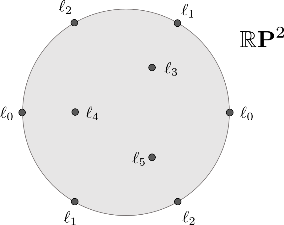
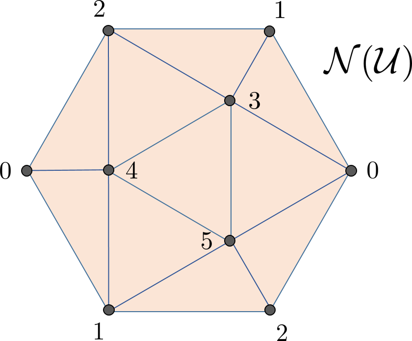
Figure 9. Left: Landmark points on $\mathbb{R}\mathbf{P}^{2}$, Right: Induced nerve complex $\mathcal{N}(\mathcal{U})$.

Let $\mathds{1}_{\{i,j\}}:\mathcal{N}(\mathcal{U})^{(1)}\longrightarrow\mathbb{Z}/2$ be the indicator function $\mathds{1}_{\{i,j\}}(\{r,k\})=1$ if $\{i,j\}=\{r,k\}$ and 0 otherwise. Then

$$\tau=\mathds{1}_{\{0,1\}}+\mathds{1}_{\{1,2\}}+\mathds{1}_{\{0,2\}}+\mathds{1}_{\{0,4\}}+\mathds{1}_{\{2,5\}}+\mathds{1}_{\{1,3\}}$$

is a 1-cocycle, and its cohomology class $[\tau]$ is the non-zero element in

$$H^{1}(\mathcal{N}(\mathcal{U});\mathbb{Z}/2)\cong\mathbb{Z}/2$$

Using the formula from Theorem 4.11, the cocycle $\tau$ above, and quadratic bumps with weights $\lambda_{j}=\epsilon_{j}^{2}$, we get the corresponding map $f_{\tau}:\mathbb{R}\mathbf{P}^{2}\longrightarrow\mathbb{R}\mathbf{P}^{5}$. For instance, if $b\in B_{\epsilon_{0}}(\ell_{0})$, then

$$f_{\tau}(b) = \left[\left|\epsilon_{0}-\mathbf{d}_{g}(b,\ell_{0})\right|_{+}\;:\;-\left|\epsilon_{1}-\mathbf{d}_{g}(b,\ell_{1})\right|_{+}\;:\;-\left|\epsilon_{2}-\mathbf{d}_{g}(b,\ell_{2})\right|_{+}\;:\;\right.$$

$$\hskip 56.9055pt\left.\left|\epsilon_{3}-\mathbf{d}_{g}(b,\ell_{3})\right|_{+}\;:\;-\left|\epsilon_{4}-\mathbf{d}_{g}(b,\ell_{4})\right|_{+}\;:\;\left|\epsilon_{5}-\mathbf{d}_{g}(b,\ell_{5})\right|_{+}\right]$$

Let $\mathbf{X}\subset\mathbb{R}\mathbf{P}^{2}$ be a uniform random sample with 10,000 points. After computing the principal projective components of $f_{\tau}(\mathbf{X})\subset\mathbb{R}\mathbf{P}^{5}$ and the percentage of cumulative variance $\mathsf{p.var}_{\mathbf{Y}}(k)$ (see equation (14)) for $k=1,\ldots,5$ we obtain the following:

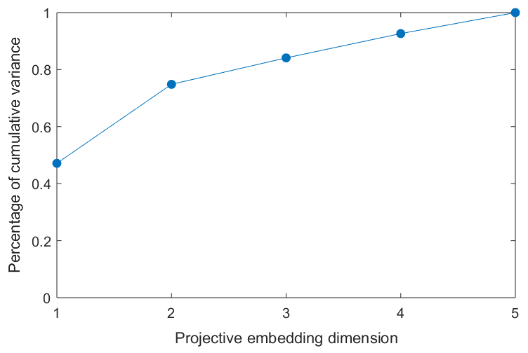
Figure 10. Percentage of cumulative variance

This profile of cumulative variance suggests that dimension 2 is appropriate for representing $f_{\tau}(\mathbf{X})$: both “the elbow” and the “70% of recovered variance” happen at around $k=2$. Below in Figure 11 we show the original sample $\mathbf{X}\subset\mathbb{R}\mathbf{P}^{2}$ as well as the point cloud $P_{V^{2}}(f_{\tau}(\mathbf{X}))$ resulting from projecting $f_{\tau}(\mathbf{X})$ onto $\mathbb{R}\mathbf{P}^{2}_{V^{2}}\subset\mathbb{R}\mathbf{P}^{5}$. Recall that $P_{V^{2}}\big{(}f_{\tau}(\mathbf{X})\big{)}$ is visualized on the unit disk $D^{2}=\{\mathbf{u}\in\mathbb{R}^{2}\,:\,\|\mathbf{u}\|\leq 1\}$, with the understanding that points in the boundary $\partial D^{2}=S^{1}$ are identified with their antipodes.

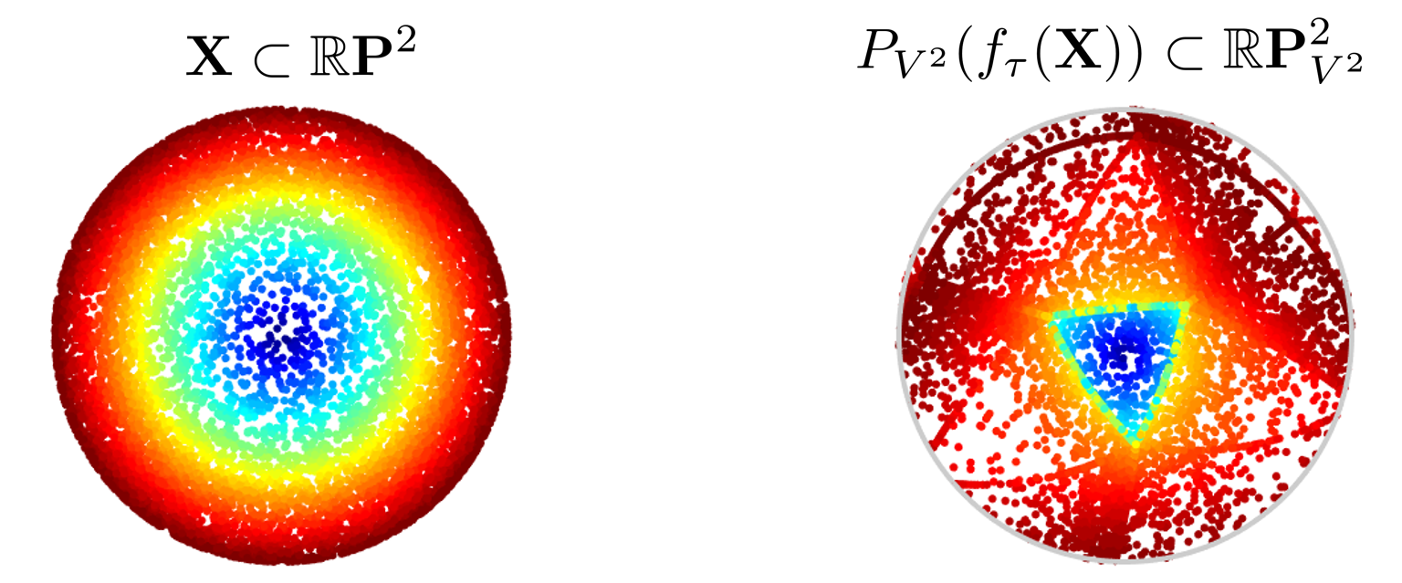
Figure 11. Left: Original sample $\mathbf{X}\subset\mathbb{R}\mathbf{P}^{2}$, Right: Visualization of resulting projective coordinates. Please refer to an electronic version for colors.

These results are consistent with the fact that any $f:\mathbb{R}\mathbf{P}^{2}\longrightarrow\mathbb{R}\mathbf{P}^{\infty}$ which classifies the nontrivial bundle over $\mathbb{R}\mathbf{P}^{2}$, must be homotopic to the inclusion $\mathbb{R}\mathbf{P}^{2}\hookrightarrow\mathbb{R}\mathbf{P}^{\infty}$. So not only did we get the right homotopy-type, but also the global geometry and the metric information were recovered to a large extent.

The Klein Bottle $K$:

Let $K$ denote the quotient of the unit square $[0,1]\times[0,1]$ by the relation $\sim$ given by $(x,0)\sim(x,1)$ and $(0,y)\sim(1,1-y)$. Let us endow $K$ with the induced flat metric, which we denote by $\mathbf{d}$, and let $\ell_{0},\ldots,\ell_{8}\in K$ be landmark points selected as shown in Figure 12(Left). If for each landmark $\ell_{j}$ we let

$$\epsilon_{j}=\min\{\mathbf{d}(\ell_{j},\ell_{r})\;:\;j\neq r\}$$

then $\mathcal{U}=\{B_{\epsilon_{j}}(\ell_{j})\}$ is a covering for $K$ and the resulting nerve complex $\mathcal{N}(\mathcal{U})$ is shown in Figure 12(Right).

Figure 12. Lef: Landmarks on the Klein bottle. Right: Induced nerve complex.

It follows that the 1-skeleton of $\mathcal{N}(\mathcal{U})$ is the complete graph on nine vertices, and that there are thirty-six 2-simplices and nine 3-simplices. Let us define the 1-chains

$$\tau_{\mathsf{diag}},\tau_{\mathsf{horz}},\tau_{\mathsf{vert}}\in C^{1}(\mathcal{N}(\mathcal{U});\mathbb{Z}/2)$$

as follows: $\tau_{\mathsf{diag}}$ will be the sum of indicator functions on the diagonal edges, $\tau_{\mathsf{horz}}$ is the sum of indicator functions on the horizontal edges, and $\tau_{\mathsf{vert}}$ will be the sum of indicator functios on the vertical edges. One can check that

$$\tau=\tau_{\mathsf{diag}}+\tau_{\mathsf{horz}}\;\;\;\;\;\mbox{ and }\;\;\;\;\;\tau^{\prime}=\tau_{\mathsf{diag}}+\tau_{\mathsf{vert}}$$

are coycles and that their cohomology classes generate

$$H^{1}(\mathcal{N}(\mathcal{U});\mathbb{Z}/2)\cong\mathbb{Z}/2\oplus\mathbb{Z}/2$$

Let $\mathbf{X}\subset K$ be a random sample with 10,000 points. The formula from Theorem 4.11 yields classifying maps

$$f_{\tau},f_{\tau^{\prime}},f_{\tau+\tau^{\prime}}:K\longrightarrow\mathbb{R}\mathbf{P}^{8}$$

and we obtain the point clouds $f_{\tau}(\mathbf{X}),f_{\tau^{\prime}}(\mathbf{X}),f_{\tau+\tau^{\prime}}(\mathbf{X})\subset\mathbb{R}\mathbf{P}^{8}$ of which we will compute their principal projective coordinates. Starting with $f_{\tau}(\mathbf{X})$ we get the profile of recovered variance shown in Figure 13.

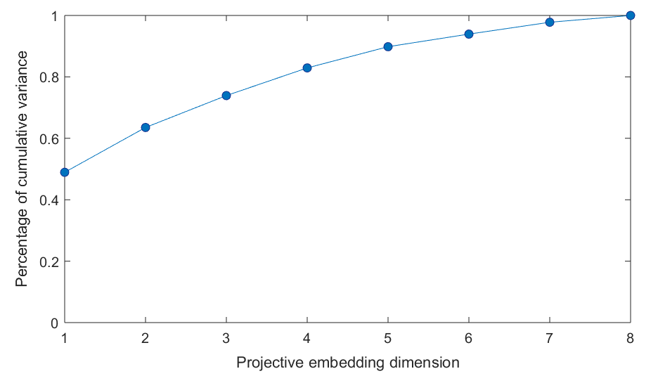
Figure 13. Percentage of cumulative variance for $f_{\tau}(\mathbf{X})$

The figure suggests that dimension 3 provides an appropriate representation of $f_{\tau}(\mathbf{X})\subset\mathbb{R}\mathbf{P}^{8}$. As described above, we visualize $P_{V^{3}}(f_{\tau}(\mathbf{X}))\subset\mathbb{R}\mathbf{P}^{3}_{V^{3}}$ in the 3-dimensional unit disk $D^{3}=\{\mathbf{u}\in\mathbb{R}^{3}\,:\,\|\mathbf{u}\|\leq 1\}$ with the understanding that points on the boundary $\partial D^{3}=S^{2}$ are identified with their antipodes. The results are summarized in Figure 14.

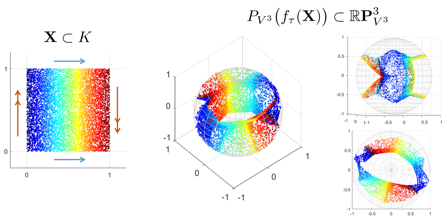
Figure 14. Left: Original sample $\mathbf{X}\subset K$; Center: Visualization of $P_{V^{3}}\big{(}f_{\tau}(\mathbf{X})\big{)}\subset\mathbb{R}\mathbf{P}^{3}_{V^{3}}$ in $D^{3}/\!\sim\;=\mathbb{R}\mathbf{P}^{3}$; Right: Lateral (upper right) and aerial view of the representation (lower right). Please refer to an electronic version for colors.

This example highlights the following point: when representing data sampled from complicated spaces, e.g. the Klein bottle, it is advantageous to use target spaces with similar properties. In particular, the representation for $\mathbf{X}\subset K$ we recover here is much simpler than those obtained with traditional dimensionality reduction methods. We now transition to the 2-dimensional reduction $P_{V^{2}}(f_{\tau}(\mathbf{X}))\subset\mathbb{R}\mathbf{P}^{2}_{V^{2}}$. As before we visualize the representation in the 2-dimensional unit disk $D^{2}$ with the understanding that points on the boundary $\partial D^{2}=S^{1}$ are identified with their antipodes.

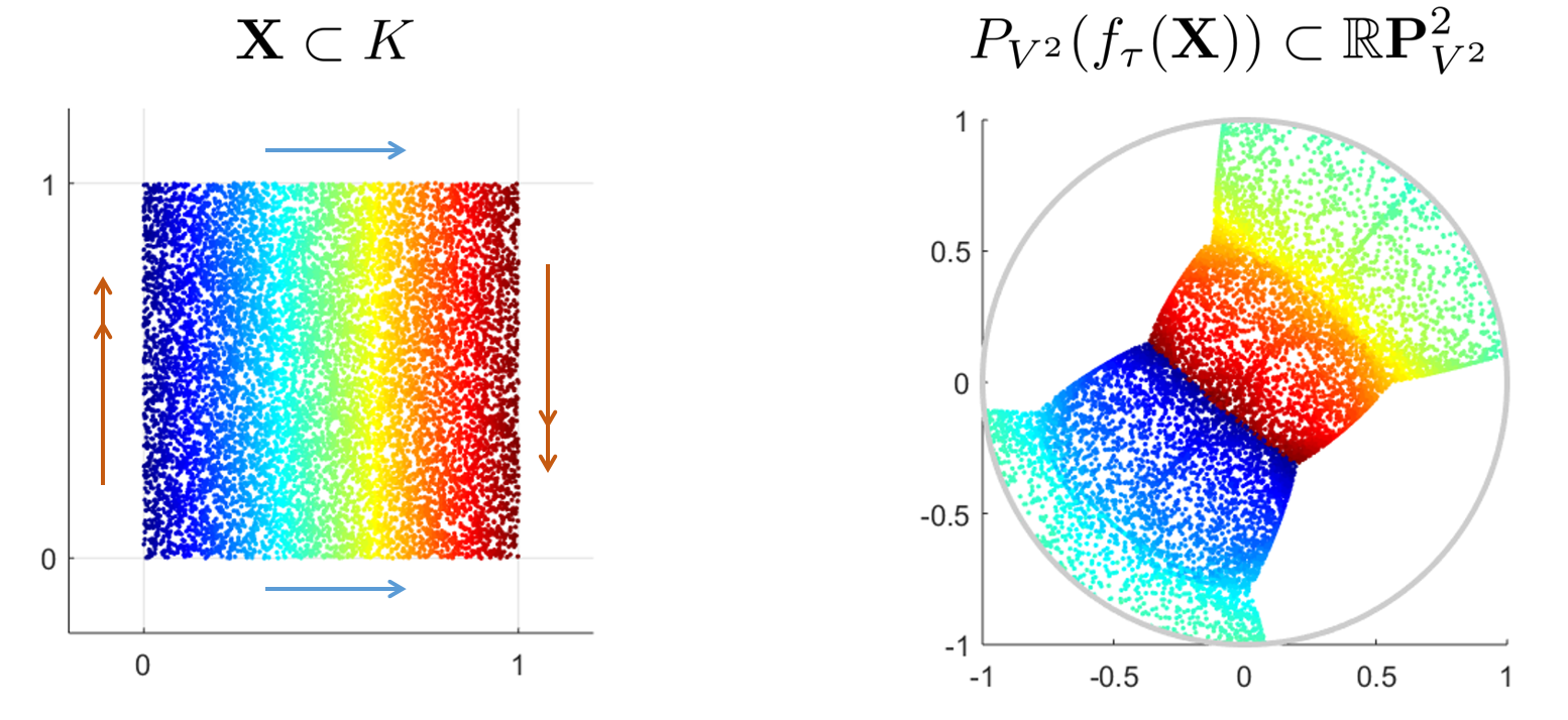
Figure 15. $\mathbb{R}\mathbf{P}^{2}$-coordinates for $\mathbf{X}\subset K$ corresponding to the cocycle $\tau$.

We conclude this example by examining the $\mathbb{R}\mathbf{P}^{2}$ coordinates induced by $\tau^{\prime}$ and $\tau+\tau^{\prime}$ (Figure 16). For completeness we include the one for $\tau$ and also add figures with coloring by the vertical direction in $K$.

Figure 16. Columns: $\mathbb{R}\mathbf{P}^{2}$ coordinates for $\mathbf{X}\subset K$ induced by the cocycles $\tau=\tau_{\mathsf{diag}}+\tau_{\mathsf{horz}}$, $\tau^{\prime}=\tau_{\mathsf{diag}}+\tau_{\mathsf{vert}}$ and $\tau+\tau^{\prime}=\tau_{\mathsf{horz}}+\tau_{\mathsf{vert}}$, respectively. Rows: Color schemes of the computed coordinates according to the horizontal and vertical directions in $K$. Please refer to an electronic version for colors.

6. Choosing Cocycle Representatives

We now describe how $f_{\tau}:B\longrightarrow\mathbb{R}\mathbf{P}^{n}$ and $f_{\eta}:B\longrightarrow\mathbb{C}\mathbf{P}^{n}$ depend on the choice of representatives $\tau=\{\tau_{rt}\}\in Z^{1}(\mathcal{N}(\mathcal{U});\mathbb{Z}/2)$ and $\eta=\{\eta_{rst}\}\in Z^{2}(\mathcal{N}(\mathcal{U});\mathbb{Z})$, respectively. We know that any two such choices yield homotopic maps (Theorem 4.11), but intricate geometries can negatively impact the dimensionality reduction step. Given $\mathbf{X}=\{\mathbf{x}_{1},\ldots,\mathbf{x}_{N}\}\subset B$, the goal is to elucidate the affects on the principal projective coordinates of $f_{\tau}(\mathbf{X})\subset\mathbb{R}\mathbf{P}^{n}$ and $f_{\eta}(\mathbf{X})\subset\mathbb{C}\mathbf{P}^{n}$. The results are: the real case is essentially independent of the cocycle representative; while the complex case requires the harmonic cocycle.

We begin with a simple observation. Let $\mathbf{Y}=\big{\{}[\mathbf{y}_{1}],\ldots,[\mathbf{y}_{N}]\big{\}}\subset\mathbb{F}\mathbf{P}^{n}$, let $A$ be a $(n+1)\times(n+1)$ orthogonal matrix with entries in $\mathbb{F}$, that is $A\in\mathsf{O}(n+1,\mathbb{F})$, and let $A\cdot\mathbf{Y}$ denote the set $\big{\{}[A\cdot\mathbf{y}_{1}],\ldots,[A\cdot\mathbf{y}_{N}]\big{\}}$.

Proposition 6.1.

Let $A\in\mathsf{O}(n+1,\mathbb{F})$ and let $\mathbf{Y}\subset\mathbb{F}\mathbf{P}^{n}$ be finite. Then

$${\tt PrinProjComps}(A\cdot\mathbf{Y})=A\cdot{\tt PrinProjComps}(\mathbf{Y})$$

Proof.

Since $A$ is an orthogonal matrix, then

$$\mathsf{Cov}(A\cdot\mathbf{Y})=A\cdot\mathsf{Cov}(\mathbf{Y})\cdot A^{\dagger}$$

Hence, if $\mathbf{u}$ is an eigenvector of $\mathsf{Cov}(\mathbf{Y})$, then $A\cdot\mathbf{u}$ is an eigenvector of $\mathsf{Cov}(A\cdot\mathbf{Y})$ with the same eigenvalue and therefore, if ${\tt LastProjComp}\left(\mathbf{Y},\mathbb{F}\mathbf{P}^{n}\right)=[\mathbf{v}_{n}]$, then

$${\tt LastProjComp}\left(A\cdot\mathbf{Y},\mathbb{F}\mathbf{P}^{n}\right)=[A\cdot\mathbf{v}_{n}]$$

Since the remaining principal projective components are computed in the same fashion, after the appropriate orthogonal projections, the result follows. ∎

The Real Case is Independent of the Cocycle Representative

Let $\alpha=\{\alpha_{r}\}\in C^{0}(\mathcal{N}(\mathcal{U});\mathbb{Z}/2)$ and let $\widetilde{\tau}=\tau+\delta^{0}(\alpha)$. It follows that for $b\in U_{j}$

$$f_{\widetilde{\tau}}(b) = \left[(-1)^{\widetilde{\tau}_{0j}}\sqrt{\varphi_{0}(b)}:\cdots:(-1)^{\widetilde{\tau}_{nj}}\sqrt{\varphi_{n}(b)}\right]$$

$$= \left[(-1)^{\tau_{0j}+\alpha_{0}}\sqrt{\varphi_{0}(b)}:\cdots:(-1)^{\tau_{nj}+\alpha_{n}}\sqrt{\varphi_{n}(b)}\right]$$

Hence, if $f_{\tau}(\mathbf{X})=\big{\{}[\mathbf{y}_{1}],\ldots,[\mathbf{y}_{N}]\big{\}}$ and

$$A_{\alpha}={\begin{bmatrix}(-1)^{\alpha_{0}}&&\mbox{\Large 0}\\ &\ddots&\\ \mbox{\Large 0}&&(-1)^{\alpha_{n}}\end{bmatrix}}$$

then $f_{\widetilde{\tau}}(\mathbf{X})=\big{\{}[A_{\alpha}\cdot\mathbf{y}_{1}],\ldots,[A_{\alpha}\cdot\mathbf{y}_{N}]\big{\}}=A_{\alpha}\cdot f_{\tau}(\mathbf{X})$. This shows that

$${\tt PrinProjComps}(f_{\widetilde{\tau}}(\mathbf{X}))=A_{\alpha}\cdot{\tt PrinProjComps}(f_{\tau}(\mathbf{X}))$$

which implies, in particular, that the profiles of cumulative variance for $f_{\widetilde{\tau}}(\mathbf{X})$ and $f_{\tau}(\mathbf{X})$ are identical. Moreover, the resulting projective coordinates for both point-clouds differ by the isometry of $\mathbb{F}\mathbf{P}^{n}$ induced by $A_{\alpha}$.

The Harmonic Representative is Required for the Complex Case

Just as we did in Section 3(Geometric Interpretation), given $\eta=\{\eta_{rst}\}\in Z^{2}(\mathcal{N}(\mathcal{U});\mathbb{Z})$ we can express $f_{\eta}:B\longrightarrow\mathbb{C}\mathbf{P}^{n}$ as

where $\varphi$ is defined in equation (10) and $F_{\eta}:|\mathcal{N}(\mathcal{U})|\longrightarrow\mathbb{C}\mathbf{P}^{n}$ is given (in barycentric coordinates) on the open star of a vertex $\mathbf{v}_{j}$ by

$$F_{\eta}(x_{0},\ldots,x_{n})=\left[\sqrt{x_{0}}\cdot e^{2\pi i\sum\limits_{t}(x_{t}\cdot\eta_{0jt})}:\cdots:\sqrt{x_{n}}\cdot e^{2\pi i\sum\limits_{t}(x_{t}\cdot\eta_{njt})}\right]$$

Let us describe the local behavior of $F_{\eta}$ when restricted to the 2-skeleton of $|\mathcal{N}(\mathcal{U})|$. To this end, let $\sigma$ be the 2-simplex of $|\mathcal{N}(\mathcal{U})|$ spanned by the vertices $\mathbf{v}_{r},\mathbf{v}_{s},\mathbf{v}_{t}$, with $0\leq r<s<t\leq n$. It follows that $F_{\eta}:\sigma\longrightarrow\mathbb{C}\mathbf{P}^{n}$ can be written as

$$F_{\eta}(x_{r},x_{s},x_{t})=\Big{[}\sqrt{x_{r}}:\sqrt{x_{s}}\cdot e^{-2\pi i\cdot\eta_{rst}\cdot x_{t}}:\sqrt{x_{t}}\cdot e^{2\pi i\cdot\eta_{rst}\cdot x_{s}}\Big{]}$$ (15)

with the understanding that only the potentially-nonzero entries appear. Furthermore, if we fix $0<c<1$ and consider the straight line in $\sigma$ given by

$$L_{c}=\Big{\{}(1-c,x,c-x)\;:\;0\leq x\leq c\Big{\}}$$

then $F_{\eta}:L_{c}\longrightarrow\mathbb{C}\mathbf{P}^{n}$ can be written as

$$F_{\eta}(x) = \Big{[}\sqrt{1-c}\;:\;\sqrt{x}\cdot e^{2\pi i(x-c)\eta_{rst}}\;:\;\sqrt{c-x}\cdot e^{2\pi i\cdot x\cdot\eta_{rst}}\Big{]}$$

$$= \Big{[}\sqrt{1-c}\cdot e^{-2\pi i\cdot x\cdot\eta_{rst}}\;:\;\sqrt{x}\cdot e^{-2\pi i\cdot c\cdot\eta_{rst}}\;:\;\sqrt{c-x}\Big{]}$$

which parametrizes a spiral with radius $\sqrt{1-c}$ and winding number $\left\lfloor c\cdot|\eta_{rst}|\right\rfloor$. Hence, as each $|\eta_{rst}|$ gets larger, $F_{\eta}$ becomes increasingly highly-nonlinear on the 2-simplices of $|\mathcal{N}(\mathcal{U})|$. As a consequence, the dimensionality reduction scheme furnished by principal projective components is less likely to work as it relies on a (global) linear approximation. Let us illustrate this phenomenon via an example.
Example: Let $B=S^{2}$ be the unit sphere in $\mathbb{R}^{3}$, and for $r\in\{0,1,2,3\}$ let $U_{r}\subset S^{2}$ be the geodesic open ball of radius $\arccos(-1/3)$ centered at

$$\ell_{0}={\begin{bmatrix}0\\ 0\\ 1\end{bmatrix}}\;\;,\;\;\ell_{1}=\frac{1}{3}{\begin{bmatrix}2\sqrt{2}\\ 0\\ -1\end{bmatrix}}\;\;,\;\;\ell_{2}=\frac{1}{3}{\begin{bmatrix}-\sqrt{2}\\ \sqrt{6}\\ -1\end{bmatrix}}\;\;,\;\;\ell_{3}=\frac{1}{3}{\begin{bmatrix}-\sqrt{2}\\ -\sqrt{6}\\ -1\end{bmatrix}}$$

respectively. It follows that $\mathcal{U}=\{U_{0},U_{1},U_{2},U_{3}\}$ is an open cover of of $S^{2}$, and that $\mathcal{N}(\mathcal{U})$ is the boundary of the 3-simplex. Therefore, if

$$\sigma_{0}=\{0,1,2\}\;\;,\;\;\sigma_{1}=\{0,2,3\}\;\;,\;\;\sigma_{2}=\{0,1,3\}\;\;,\;\;\sigma_{3}=\{1,2,3\}$$

denote the 2-simplices of $\mathcal{N}(\mathcal{U})$ and $\{\eta^{0},\eta^{1},\eta^{2},\eta^{3}\}$ is the basis for $C^{2}(\mathcal{N}(\mathcal{U});\mathbb{Z})$ of indicator functions, then each $\eta^{r}$ is a cocycle whose cohomology class generates

$$H^{2}(\mathcal{N}(\mathcal{U});\mathbb{Z})\cong\mathbb{Z}$$

Moreover, $\big{\{}\eta^{0}-\eta^{1}\;,\;\eta^{0}+\eta^{2}\;,\;\eta^{0}+\eta^{3}\big{\}}$ is a basis for $B^{2}(\mathcal{N}(\mathcal{U});\mathbb{Z})$ and therefore

$$[\eta^{0}]=[\eta^{1}]=-[\eta^{2}]=-[\eta^{3}]$$

Consider the map $f_{\eta}:S^{2}\longrightarrow\mathbb{C}\mathbf{P}^{3}$ associated to $\eta=\eta^{0}$; the results will be similar for the other $\eta^{r}$’s. We show in Figure 17 the computed $\mathbb{C}\mathbf{P}^{1}$ coordinates of $f_{\eta}(\mathbf{X})$ for a random sample $\mathbf{X}\subset S^{2}$ with 10,000 points. As one can see, the homotopy type of the resulting map is correct, but the distances are completely distorted.

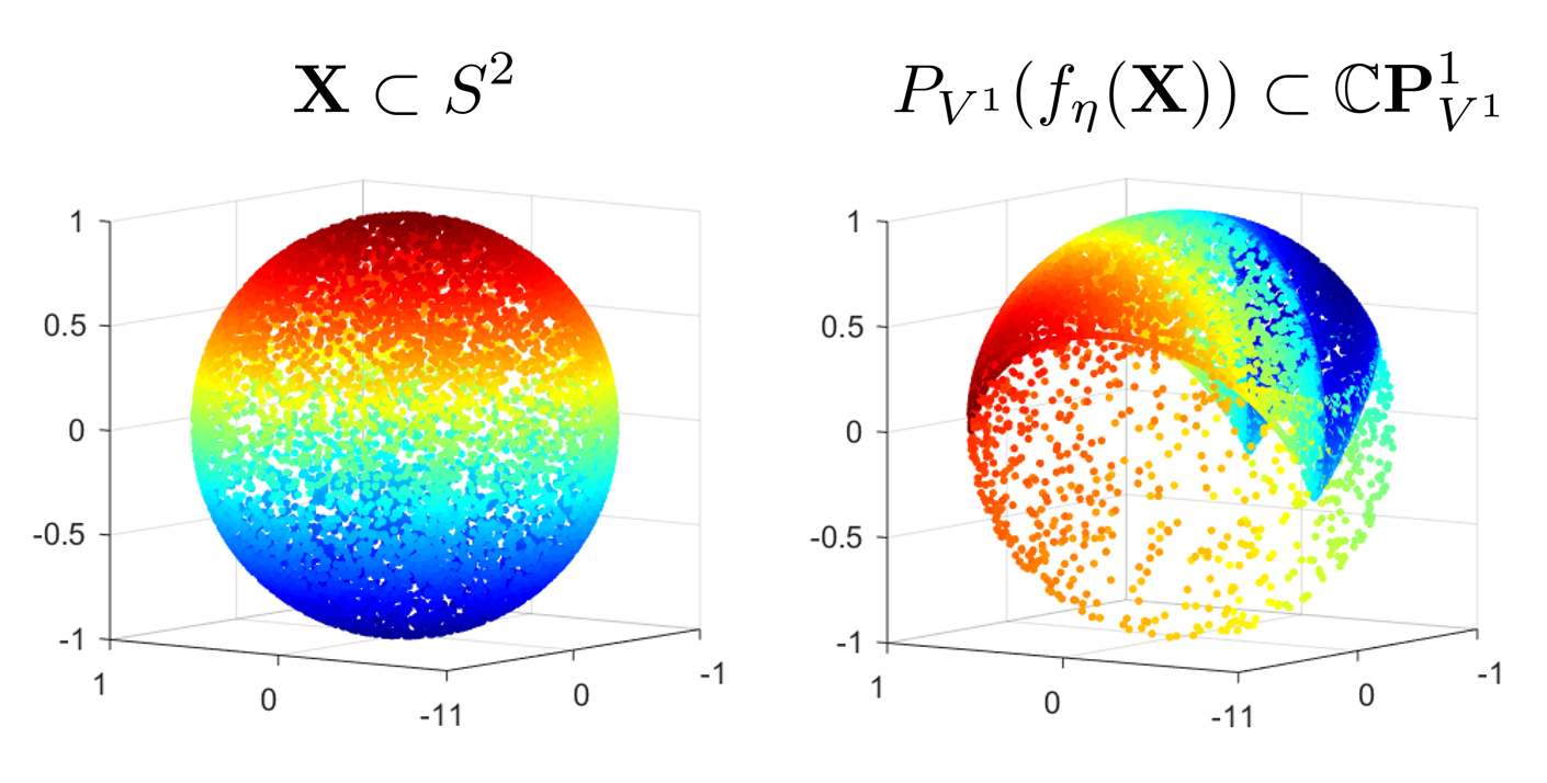
Figure 17. $\mathbb{C}\mathbf{P}^{1}$ coordinates for points on the 2-sphere using the map $f_{\eta}$ associated to the integer cocycle $\eta=\eta^{0}$. This shows the inadequacy of the integer cocycle; see Figure 18 for comparison. Please refer to an electronic version for colors.

The main difference between the real and complex cases is that the former is locally linear, while the latter has local nonlinearities arising from the terms

$$\exp\big{(}2\pi i\cdot\eta_{rst}\cdot x_{t}\big{)}.$$

The tempting conclusion would be then to choose the cocycle representative $\eta=\{\eta_{rst}\}\in Z^{2}(\mathcal{N}(\mathcal{U});\mathbb{Z})$ that makes $F_{\eta}$ as locally linear as possible. This can be achieved by making each $|\eta_{rst}|$ small. The problem — as in the sphere example — is that since $\eta_{rst}\in\mathbb{Z}$, then even this choice is inadequate. What we will see now is that the integer constraint can be relaxed via Hodge theory (see, for instance, Section 2 of [24]).

Harmonic Smoothing

Let $K$ be a finite simplicial complex. Then for each $n\geq 0$ the group of $n$-cochains $C^{n}(K;\mathbb{R})$ is a finite dimensional vector space over $\mathbb{R}$, and hence can be endowed with an inner product. A common choice is

$$\langle\beta_{1},\beta_{2}\rangle_{n}=\sum_{\sigma}\beta_{1}(\sigma)\beta_{2}(\sigma)$$

where $\beta_{1},\beta_{2}\in C^{n}(K;\mathbb{R})$ and the sum ranges over all $n$-simplices $\sigma$ of $K$. In particular we have the induced norm

$$\|\beta\|^{2}=\sum_{\sigma}|\beta(\sigma)|^{2}$$

Each boundary map $\delta^{n}:C^{n}(K;\mathbb{R})\longrightarrow C^{n+1}(K;\mathbb{R})$ is therefore a linear transformation between inner-product spaces, and hence has an associated dual map $d_{n+1}:C^{n+1}(K;\mathbb{R})\longrightarrow C^{n}(K;\mathbb{R})$ uniquely determined by the identity

$$\left\langle\,\delta^{n}(\nu)\;,\;\beta\,\right\rangle_{n+1}=\left\langle\,\nu\;,\;d_{n+1}(\beta)\,\right\rangle_{n}$$

for all $\nu\in C^{n}(K;\mathbb{R})$ and all $\beta\in C^{n+1}(K;\mathbb{R})$. The Hodge Laplacian $\Delta_{n}$ is the endomorphism of $C^{n}(K;\mathbb{R})$ defined by the formula

$$\Delta_{n}=d_{n+1}\circ\delta^{n}\;+\;\delta^{n-1}\circ d_{n}$$

and a cochain $\theta\in C^{n}(K;\mathbb{R})$ is said to be harmonic if $\Delta_{n}(\theta)=0$. A simple linear algebra argument shows that Harmonic cochains can be characterized as follows:

Proposition 6.2.

$\theta\in C^{n}(K;\mathbb{R})$ is harmonic if and only if

$$d_{n}(\theta)=0\;\;\;\mbox{ and }\;\;\;\delta^{n}(\theta)=0.$$

That is, harmonic cochains are in particular cocycles. Moreover

Theorem 6.3.

Every class $[\beta]\in H^{n}(K;\mathbb{R})$ is represented by a unique harmonic cocycle $\theta\in Z^{n}(K;\mathbb{R})$ satisfying $\theta=\beta-\delta^{n-1}(\nu^{*})$, where

$$\nu^{*}=\operatorname*{\arg\!\min\;}\big{\{}\left\|\beta-\delta^{n-1}(\nu)\right\|:\nu\in C^{n-1}(K;\mathbb{R})\big{\}}$$

In other words, given $\beta\in Z^{n}(K;\mathbb{R})$, $\theta$ is obtained by projecting $\beta$ orthogonally onto the orthogonal complement of $B^{n}(K;\mathbb{R})$ in $Z^{n}(K;\mathbb{R})$.
Let us now go back to our original set up: A covering $\mathcal{U}=\{U_{r}\}$ for a space $B$, a partition of unity $\{\varphi_{r}\}$ dominated by $\mathcal{U}$ and a class $[\eta]\in H^{2}(\mathcal{N}(\mathcal{U});\mathbb{Z})$. The inclusion $\jmath:\mathbb{Z}\hookrightarrow\mathbb{R}$ induces a homomorphism

$$\jmath^{*}:H^{2}(\mathcal{N}(\mathcal{U});\mathbb{Z})\longrightarrow H^{2}(\mathcal{N}(\mathcal{U});\mathbb{R})$$

and if $\beta\in\jmath^{*}([\eta])$, then there exists $\nu\in C^{1}(\mathcal{N}(\mathcal{U});\mathbb{R})$ so that $\jmath^{\#}(\eta)=\beta+\delta^{1}(\nu)$.

Lemma 6.4.

Let $\omega=\{\omega_{rs}\}$ and $\widetilde{\omega}=\{\widetilde{\omega}_{rs}\}$ be the sets of functions

$$\begin{array}[]{cccl}\omega_{rs}:&U_{r}\cap U_{s}&\longrightarrow&\mathbb{C}^{\times}\\ &b&\mapsto&\exp\left\{2\pi i\sum\limits_{t}\varphi_{t}(b)\eta_{rst}\right\}\\ \\ \widetilde{\omega}_{rs}:&U_{r}\cap U_{s}&\longrightarrow&\mathbb{C}^{\times}\\ &b&\mapsto&\exp\left\{2\pi i\left(\nu_{rs}+\sum\limits_{t}\varphi_{t}(b)\beta_{rst}\right)\right\}\end{array}$$

then $\omega,\widetilde{\omega}\in\check{C}^{1}(\mathcal{U};\mathscr{C}_{\mathbb{C}}^{\times})$ are cohomologous Čech cocycles.

Proof.

Since $\omega$ is a cocycle, it is enough that check that $\omega$ and $\widetilde{\omega}$ are cohomologous. To this end let $\mu=\{\mu_{r}\}\in\check{C}^{0}(\mathcal{U};\mathscr{C}_{\mathbb{C}}^{\times})$, where

$$\mu_{r}(b)=\exp\left\{2\pi i\sum_{t}\varphi_{t}(b)\cdot\nu_{rt}\right\}\;\;\;\;b\in U_{r}$$

Since for every $U_{r}\cap U_{t}\neq\emptyset$

$$\sum_{t}\varphi_{t}\cdot n_{rst} = \sum_{t}\varphi_{t}\cdot\left(\beta_{rst}+\delta^{1}(\nu)_{rst}\right)$$

$$= \sum_{t}\varphi_{t}\cdot(\beta_{rst}+\nu_{rs}-\nu_{rt}+\nu_{st})$$

$$= \nu_{rs}+\sum_{t}\varphi_{t}\cdot\beta_{rst}+\sum_{t}\varphi_{t}\cdot\nu_{st}-\sum_{t}\varphi_{t}\cdot\nu_{rt}$$

then

$$\omega_{rs}=\widetilde{\omega}_{rs}\cdot\frac{\mu_{s}}{\mu_{r}}=\widetilde{\omega}_{rs}\cdot\delta^{0}(\mu)_{rs}$$

and the result follows. ∎

Let $\theta\in Z^{2}(\mathcal{N}(\mathcal{U});\mathbb{R})$ be the harmonic cocycle representing the class

$$\jmath^{*}([\eta])\in H^{2}(\mathcal{N}(\mathcal{U});\mathbb{R})$$

let $\nu\in C^{1}(\mathcal{N}(\mathcal{U});\mathbb{R})$ be so that $\jmath^{\#}(\eta)-\theta=\delta^{1}(\nu)$ and let $f_{\theta,\nu}:B\longrightarrow\mathbb{C}\mathbf{P}^{n}$ be given on $b\in U_{j}$

$$f_{\theta,\nu}(b)=\left[\sqrt{\varphi_{0}(b)}\cdot e^{2\pi i\big{(}\nu_{0j}+\sum\limits_{t}\varphi_{t}(b)\theta_{0jt}\big{)}}:\cdots:\sqrt{\varphi_{n}(b)}\cdot e^{2\pi i\big{(}\nu_{nj}+\sum\limits_{t}\varphi_{t}(b)\theta_{njt}\big{)}}\right]$$ (16)

It follows that $f_{\eta}$ and $f_{\theta,\nu}$ are homotopic, $f_{\theta,\nu}$ is as locally linear as possible, and for different choices of $\nu$ the resulting principal projective coordinates of $f_{\theta,\nu}(\mathbf{X})$ differ by a linear (diagonal) isometry.

We now revisit the 2-sphere example. One can check that

$$\theta=\jmath^{\#}\left(\eta^{0}+\eta^{1}-\eta^{2}-\eta^{3}\right)/4$$

is the harmonic cocycle representing the cohomology class

$$\jmath^{*}\left(\left[\eta^{0}\right]\right)\in H^{2}(\mathcal{N}(\mathcal{U});\mathbb{R})$$

Let $\nu\in C^{1}(\mathcal{N}(\mathcal{U});\mathbb{R})$ be so that $\theta=\jmath^{\#}(\eta^{0})-\delta^{1}(\nu)$ and let $f_{\theta,\nu}:S^{2}\longrightarrow\mathbb{C}\mathbf{P}^{3}$ be as in equation (16). We show in Figure 18 the computed $\mathbb{C}\mathbf{P}^{1}$ coordinates of $f_{\theta,\nu}(\mathbf{X})$ for the finite random sample $\mathbf{X}\subset S^{2}$.

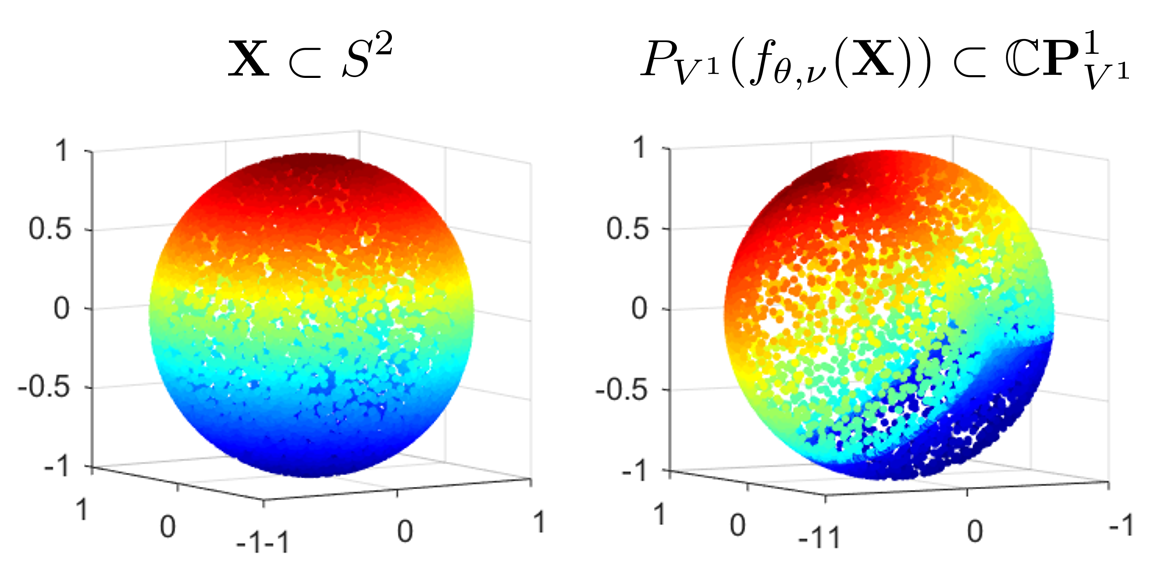
Figure 18. $\mathbb{C}\mathbf{P}^{1}$ coordinates for $\mathbf{X}\subset S^{2}$ using the harmonic cocycle $\theta$; see Figure 17 for comparison. Please refer to an electronic version for colors.

7. Multiscale Projective Coordinates via Persistent Cohomology of Sparse Filtrations

The goal of this section is to show how one can use persistent cohomology to construct multiscale projective coordinates.

Greedy Permutations

Let $\underline{k}=\{0,\ldots,k\}$ for $k\in\mathbb{Z}_{\geq 0}$, let $(\mathbb{M},\mathbf{d})$ be a metric space and let $X\subset\mathbb{M}$ be a finite subset with $n+1$ elements. A greedy permutation on $X$ is a bijection $\sigma_{g}:\underline{n}\longrightarrow X$ which satisfies

$$\sigma_{g}(s+1)=\operatorname*{\arg\!\max\;}\limits_{x\in X}\mathbf{d}\big{(}x,\sigma_{g}\left(\underline{s}\right)\big{)}\;\;,\;\;\;s=0,\ldots,n-1$$

Sparse Filtrations

Given a greedy permutation $\sigma_{g}:\underline{n}\longrightarrow X$, let $x_{s}=\sigma_{g}(s)$ and $X_{s}=\sigma_{g}\left(\underline{s}\right)$. The insertion radius of $x_{s}$, denoted $\lambda_{s}$, is defined as

$$\lambda_{s}=\left\{\begin{array}[]{ccc}\infty&\mbox{ if }&s=0\\[5.69046pt] \mathbf{d}\big{(}x_{s},X_{s-1}\big{)}&\mbox{ if }&s>0\end{array}\right.$$

If follows that $\infty=\lambda_{0}>\lambda_{1}\geq\cdots\geq\lambda_{n}$ . Fix $0<\epsilon<1$ and for $\alpha\geq 0$ define

$$r_{s}(\alpha)=\left\{\begin{array}[]{ccc}\alpha&\hbox{ if }&\alpha<\lambda_{s}(1+\epsilon)/\epsilon\\[5.69046pt] \lambda_{s}(1+\epsilon)/\epsilon&\hbox{ if }&\lambda_{s}(1+\epsilon)/\epsilon\leq\alpha\leq\lambda_{s}(1+\epsilon)^{2}/\epsilon\\[5.69046pt] 0&\hbox{ if }&\alpha>\lambda_{s}(1+\epsilon)^{2}/\epsilon\end{array}\right.$$ (17)

In particular $r_{0}(\alpha)=\alpha$ for all $\alpha\geq 0$, and for $s\geq 1$ the graph of $r_{s}$ is shown below.

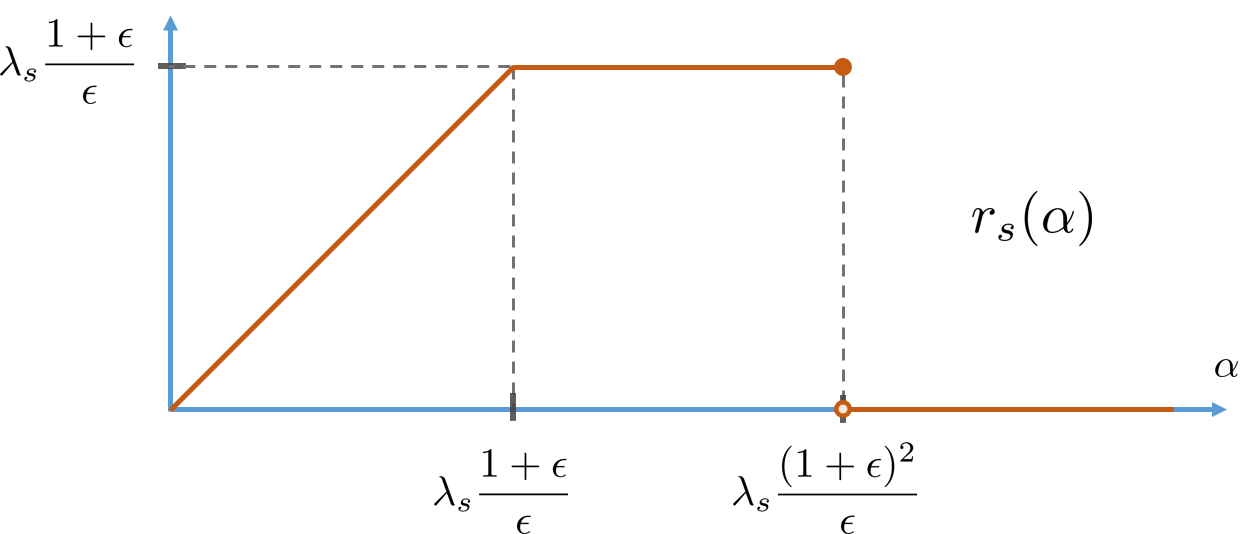
Figure 19. Function $r_{s}$

Definition 7.1.

For $\alpha\geq 0$ let

$$B_{s}^{\alpha}=\{b\in\mathbb{M}\;:\;\mathbf{d}(b,x_{s})<r_{s}(\alpha)\}$$

It follows thats $S_{\alpha}=\left\{s\in\underline{n}\;:\;\lambda_{s}\geq\epsilon\alpha/(1+\epsilon)^{2}\right\}$ is the collection of indices $s$ for which $B_{s}^{\alpha}\neq\emptyset$. Moreover,

$$\mathcal{B}^{\alpha}=\{B_{s}^{\alpha}\;:\;s\in S_{\alpha}\}$$

satisfies $X\subset\bigcup\mathcal{B}^{\alpha}$ for each $\alpha>0$, and it is a sparse covering in the sense that as $\alpha$ increases there are fewer balls in $\mathcal{B}^{\alpha}$, but of larger radii. Moreover, it is a $(1+\epsilon)$-approximation of the $\alpha$-offset $X^{\alpha}=\{b\in\mathbb{M}\;:\;\mathbf{d}(b,X)<\alpha\}$:

Proposition 7.2 ([6], Corollary 2).

If $\beta\geq(1+\epsilon)\alpha$, then

$$\bigcup\mathcal{B}^{\alpha}\subset X^{\alpha}\subset\bigcup\mathcal{B}^{\beta}$$

Let

$$U^{\alpha}_{s}=\bigcup_{0\leq\lambda\leq\alpha}\big{(}B_{s}^{\lambda}\times\{\lambda\}\big{)}\;\;\;\mbox{ and }\;\;\;\mathcal{U}^{\alpha}=\left\{U_{s}^{\alpha}\;:\;s\in\underline{n}\right\}$$

It follows that $\mathcal{N}(\mathcal{U}^{\alpha})\subset\mathcal{N}(\mathcal{U}^{\beta})$ whenever $\alpha\leq\beta$.

Definition 7.3.

The sparse Čech filtration with sparsity parameter $0<\epsilon<1$, induced by the greedy permutation $\sigma_{g}:\underline{n}\longrightarrow X$, is the filtered simplicial complex

$$\check{\mathcal{C}}(\sigma_{g},\epsilon)=\left\{\check{C}_{\alpha}(\sigma_{g},\epsilon)\;:\;\alpha\geq 0\right\}$$

where

$$\check{\mathcal{C}}_{\alpha}(\sigma_{g},\epsilon)=\mathcal{N}\left(\mathcal{U}^{\alpha}\right)$$

Multiscale Projective Coordinates

We will show now how the persistent cohomology of $\check{\mathcal{C}}(\sigma_{g},\epsilon)$ can be used to compute multiscale compatible classifying maps. The first thing to notice is that projection onto the first coordinate

$$\begin{array}[]{ccc}\bigcup\mathcal{U}^{\alpha}&\longrightarrow&\bigcup\mathcal{B}^{\alpha}\\[2.84544pt] (b,\lambda)&\mapsto&b\end{array}$$

is a deformation retraction if one regards $B_{s}^{\alpha}$ as a subset of $U_{s}^{\alpha}$ via the inclusion

$$\begin{array}[]{ccc}B_{s}^{\alpha}&\hookrightarrow&U^{\alpha}_{s}\\ b&\mapsto&(b,\alpha)\end{array}$$ (18)

Theorem 7.4.

Let $(\mathbb{M},\mathbf{d})$ be a metric space and let $X\subset\mathbb{M}$ be a subset with $n+1$ points. Given a greedy permutation $\sigma_{g}:\underline{n}\longrightarrow X$ and a sparsity parameter $0<\epsilon<1$, let $r_{s}(\alpha)$ for $\alpha\geq 0$ be as in equation (17).

If $\check{\mathcal{C}}(\sigma_{g},\epsilon)$ is the resulting sparse Čech filtration and

$$\varphi^{\alpha}_{s}(b)=\frac{\left|r_{s}(\alpha)-\mathbf{d}(b,x_{s})\right|_{+}^{2}}{\sum\limits_{t\in\underline{n}}\left|r_{t}(\alpha)-\mathbf{d}(b,x_{t})\right|_{+}^{2}}\;\;\;\;\;\;\mbox{ for }\;\;\;\;\;\;\;s\in\underline{n}\;\;,\;\;b\in\bigcup\mathcal{B}^{\alpha}$$

then we have well-defined maps

$$\begin{array}[]{rccl}\mathbf{w}^{\alpha}_{1}:&H^{1}\left(\check{\mathcal{C}}_{\alpha}(\sigma_{g},\epsilon);\mathbb{Z}/2\right)&\longrightarrow&\left[\bigcup\mathcal{B}^{\alpha}\,,\,\mathbb{R}\mathbf{P}^{\infty}\right]\\[5.69046pt] &[\tau=\{\tau_{rt}\}]&\mapsto&[f^{\alpha}_{\tau}]\\ \\ f^{\alpha}_{\tau}:&\bigcup\mathcal{B}^{\alpha}&\longrightarrow&\mathbb{R}\mathbf{P}^{n}\\ &B^{\alpha}_{j}\ni b&\mapsto&\left[(-1)^{\tau_{0j}}\sqrt{\varphi^{\alpha}_{0}(b)}:\cdots:(-1)^{\tau_{nj}}\sqrt{\varphi^{\alpha}_{n}(b)}\right]\end{array}$$

and

$$\begin{array}[]{rccl}\mathbf{c}^{\alpha}_{1}:&H^{2}\left(\check{\mathcal{C}}_{\alpha}(\sigma_{g},\epsilon);\mathbb{Z}\right)&\longrightarrow&\left[\bigcup\mathcal{B}^{\alpha}\,,\,\mathbb{C}\mathbf{P}^{\infty}\right]\\[5.69046pt] &\left[\eta=\theta+\delta^{1}(\nu)\right]&\mapsto&[f^{\alpha}_{\theta,\nu}]\\ \\ f^{\alpha}_{\theta,\nu}:&\bigcup\mathcal{B}^{\alpha}&\longrightarrow&\mathbb{C}\mathbf{P}^{n}\\ &B^{\alpha}_{j}\ni b&\mapsto&\left[e^{2\pi i(\nu_{0j}+\sum\limits_{t}\varphi^{\alpha}_{t}(b)\theta_{0jt})}\sqrt{\varphi^{\alpha}_{0}(b)}:\cdots:e^{2\pi i(\nu_{nj}+\sum\limits_{t}\varphi^{\alpha}_{t}(b)\theta_{njt})}\sqrt{\varphi^{\alpha}_{n}(b)}\right]\end{array}$$

where $\theta=\{\theta_{rst}\}\in Z^{2}\left(\check{C}_{\alpha}(\sigma_{g},\epsilon);\mathbb{R}\right)$ is the harmonic cocycle representing $\jmath^{*}([\eta])\in H^{2}\left(\check{C}_{\alpha}(\sigma_{g},\epsilon);\mathbb{R}\right)$ and $\nu=\{\nu_{rt}\}\in C^{1}\left(\check{C}_{\alpha}(\sigma_{g},\epsilon);\mathbb{R}\right)$ is so that $\theta=\jmath^{\#}(\eta)-\delta^{1}(\nu)$. Moreover, if each $B^{\alpha}_{s}\in\mathcal{B}^{\alpha}$ is connected, then $\mathbf{w}_{1}^{\alpha}$ is injective; if in addition each $B^{\alpha}_{s}$ is locally path-connected and simply connected, and each $B^{\alpha}_{r}\cap B^{\alpha}_{t}$ is either empty or connected, then $\mathbf{c}_{1}^{\alpha}$ is injective.

Proof.

The first thing to notice is that the collection of continuous maps

$$\begin{array}[]{rccl}\varphi_{s}&:\bigcup\mathcal{U}^{\alpha}&\longrightarrow&\mathbb{R}\\ &(b,\lambda)&\mapsto&\varphi_{s}^{\lambda}(b)\end{array}\;\;\;\;\;,\;\;\;\;s\in\underline{n}$$

is a partition of unity dominated by $\mathcal{U}^{\alpha}$. The Theorem follows from combining Theorem 4.11 and the following two facts: the inclusion $\bigcup\mathcal{B}^{\alpha}\hookrightarrow\bigcup\mathcal{U}^{\alpha}$ from Equation (18) induces a bijection

$$\left[\bigcup\mathcal{U}^{\alpha},\mathbb{F}\mathbf{P}^{\infty}\right]\longrightarrow\left[\bigcup\mathcal{B}^{\alpha},\mathbb{F}\mathbf{P}^{\infty}\right]$$

and the necessary connectedness conditions are satisfied by $\mathcal{U}^{\alpha}$ if they are satisfied by $\mathcal{B}^{\alpha}$. ∎

Remark 7.5.

As $\alpha$ increases, the number of potentially nontrivial dimensions in the images of $f_{\tau}^{\alpha}$ and $f_{\theta,\nu}^{\alpha}$ decrease. Indeed, since $\varphi_{s}^{\alpha}$ is identically zero if and only if $B_{s}^{\alpha}=\emptyset$, it follows that for any $b\in\bigcup\mathcal{B}^{\alpha}$ the only potentially non-zero entries in either $f^{\alpha}_{\tau}(b)$ or $f^{\alpha}_{\theta,\nu}(b)$ correspond to the indices in

$$S_{\alpha}=\{s\in\underline{n}\;:\;\lambda_{s}\geq\epsilon\alpha/(1+\epsilon)^{2}\}$$

The observation follows from the fact that the sequence $\{\lambda_{s}\}_{s\in\underline{n}}$ is non-increasing, and monotonically decreasing for generic $X$.

Proposition 7.6.

Let $\alpha\leq\beta$, then the diagrams

are commutative.

As a consequence, if for $\alpha=\alpha_{0}<\cdots<\alpha_{\ell-1}<\alpha_{\ell}=\beta$ one has classes

then the diagram

commutes up to a homotopy which perhaps takes place in a higher dimensional projective space. The same is true in dimension one with $\mathbb{Z}/2$ coefficients. The persistent cohomology of the sparse Čech filtration $\check{\mathcal{C}}(\sigma_{g},\epsilon)$ now becomes relevant: over $\mathbb{Z}/2$, a 1-dimensional cohomology class with nonzero persistence yields a multiscale system of compatible (up to homotopy) $\mathbb{R}\mathbf{P}^{n}$ coordinates. Constructing multiscale $\mathbb{C}\mathbf{P}^{n}$ coordinates from a persistent cohomology computation for $k=2$ requires a bit more work, as the barcode decomposition is not valid for integer coefficients. Let $p$ be a prime and consider the short exact sequence of abelian groups

The induced homomorphism

$$H^{2}\left(\mathcal{\check{C}}_{\alpha}(\sigma_{g},\epsilon);\mathbb{Z}\right)\longrightarrow H^{2}\left(\mathcal{\check{C}}_{\alpha}(\sigma_{g},\epsilon);\mathbb{Z}/p\right)$$

will be an epimorphism whenever $H^{3}\left(\mathcal{\check{C}}_{\alpha}(\sigma_{g},\epsilon);\mathbb{Z}\right)$ has no $p$-torsion. The universal coefficient theorem implies the following

Proposition 7.7.

Let $p$ be a prime not dividing the order of the torsion subgroup of $H_{2}(\mathcal{\check{C}}_{\alpha}(\sigma_{g},\epsilon);\mathbb{Z})$. Then the homomorphism

$$H^{2}(\mathcal{\check{C}}_{\alpha}(\sigma_{g},\epsilon);\mathbb{Z})\longrightarrow H^{2}(\mathcal{\check{C}}_{\alpha}(\sigma_{g},\epsilon);\mathbb{Z}/p)$$

is surjective.

Now one can follow the strategy in [13, Sections 2.4 and 2.5] for choosing $p$, lifting to integer coefficients and constructing the harmonic representative. The solution to the harmonic representative problem is plugged into equation (16).

Definition 7.8.

The sparse Rips filtration, with sparsity parameter $0<\epsilon<1$, induced by the greedy permutation $\sigma_{g}:\underline{n}\longrightarrow X$ is the filtered simplicial complex

$$\mathcal{R}(\sigma_{g},\epsilon)=\big{\{}R_{\alpha}(\sigma_{g},\epsilon)\;:\;\alpha\geq 0\big{\}}$$

where

$$R_{\alpha}(\sigma_{g},\epsilon)=\big{\{}\{s_{0},\ldots,s_{k}\}\subset\underline{n}\;:\;U_{s_{r}}^{\alpha}\cap U_{s_{t}}^{\alpha}\neq\emptyset\mbox{ for all }0\leq r,t\leq k\big{\}}$$

Remark 7.9.

It follows that for all $\beta\geq 0$

$$\check{C}_{\beta}(\sigma_{g},\epsilon)\subset R_{\beta}(\sigma_{g},\epsilon)$$

and if $\alpha$ is small enough (as the cones $U_{s}^{\alpha}$ stop growing) we also get the inclusion $R_{\alpha}(\sigma_{g},\epsilon)\subset\check{C}_{2\alpha}(\sigma_{g},\epsilon).$ Then for each abelian group $G$ and integer $k\geq 0$ we get a commutative diagram

which shows that cohomology classes in the sparse Rips filtration with long enough persistence, and small enough death time, yield nontrivial persistent cohomology classes in the sparse Čech filtration. This is useful because the persistent cohomology of the sparse Rips filtration is easier to compute in practice.

Example:

Let $\mathbf{X}$ be a uniform random sample with $2,500$ points from the 2-dimensional torus $S^{1}\times S^{1}\subset\mathbb{C}^{2}$, endowed with the metric $\mathbf{d}$ given by

$$\mathbf{d}\big{(}(z_{1},w_{1}),(z_{2},w_{2})\big{)}=\sqrt{\big{|}\arccos(\langle z_{1},z_{2}\rangle)\big{|}^{2}+\big{|}\arccos(\langle w_{1},w_{2}\rangle)\big{|}^{2}}$$

There are two things we would like to illustrate with this example: First, that one does not need the entire data set $\mathbf{X}$ to compute appropriate classifying maps $f^{\alpha}_{\tau}$, in fact a small subsample suffices; and second, that one can use the sparse Rips filtration instead of the Čech filtration, which simplifies computations. Indeed, let $n=34$ and let

$$X=\{x_{0},\ldots,x_{n}\}\subset\mathbf{X}$$

be obtained through maxmin sampling. Notice that $X$ is $1.4\%$ of the total size of $\mathbf{X}$ and that $\sigma_{g}:\underline{n}\longrightarrow X$ given by $\sigma_{g}(s)=x_{s}$ is a greedy permutation on $X$. We let $\epsilon=0.01$ since the sample is already sparse. Computing the 1-dimensional persistent cohomology with coefficients in $\mathbb{Z}/2$ for the sparse Rips filtration $\mathcal{R}(\sigma_{g},\epsilon)$, yields the barcode shown in Figure 20(left).

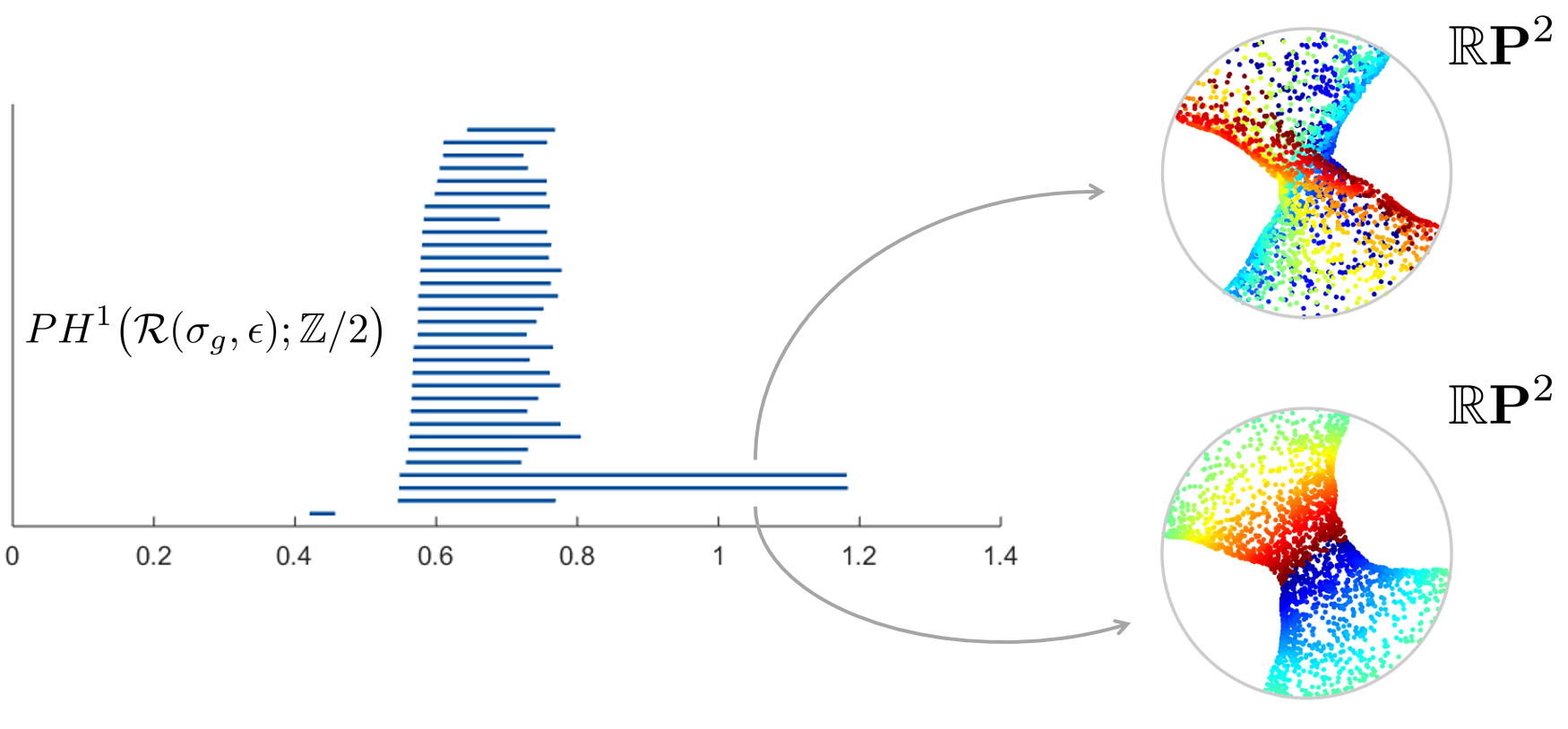
Figure 20. $\mathbb{R}\mathbf{P}^{2}$ coordinates for $\mathbf{X}\subset S^{1}\times S^{1}$, from the 1-dimensional $\mathbb{Z}/2$-persistent cohomology of a sparse rips filtration. Left: Computed barcode, Right: resulting $\mathbb{R}\mathbf{P}^{2}$ coordinates induced by classes with large persistence. In both cases, the $\mathbb{R}\mathbf{P}^{2}$ coordinates of a point $(z,w)\in\mathbf{X}$ are colored according to $\arg(z)\in[0,2\pi)$. Please refer to an electronic version for colors.

For this calculation we first determine the birth-times of the edges as in [6, Algorithm 3], and input them as a distance matrix into Dionysus’ persistent cohomology algorithm [29]. After selecting the two classes with the longest persistence, Dionysus outputs cocycle representatives $\mu_{1}$ and $\mu_{2}$ at cohomological birth $\alpha_{1},\alpha_{2}\approx 1.18$. Now, using the fact that $\check{C}_{\alpha}(\sigma_{g},\epsilon)\subset R_{\alpha}(\sigma_{g},\epsilon)$ for all $\alpha\geq 0$, we have that the induced homomorphism

$$C^{1}(R_{\alpha}(\sigma_{g},\epsilon);\mathbb{Z}/2)\longrightarrow C^{1}(\check{C}_{\alpha}(\sigma_{g},\epsilon);\mathbb{Z}/2)$$

sends $\mu_{1}$ and $\mu_{2}$ to $\tau_{1}$ and $\tau_{2}$, respectively. Moreover, since $R_{\alpha}(\sigma_{g},\epsilon)$ is connected at $\alpha=\min\{\alpha_{1},\alpha_{2}\}$ it follows that $\mathbf{X}\subset\bigcup\mathcal{B}^{\alpha}$, and using the formula from Theorem 7.4 we get the point clouds $f_{\tau_{1}}^{\alpha}(\mathbf{X}),f_{\tau_{2}}^{\alpha}(\mathbf{X})\subset\mathbb{R}\mathbf{P}^{34}$. The result of computing their $\mathbb{R}\mathbf{P}^{2}$ coordinates via principal projective components is shown in Figure 20(right).

8. Discussion

We have shown in this paper how 1-dimensional (resp. 2-dimensional) persistent cohomology classes with $\mathbb{Z}/2$ coefficients (resp. $\mathbb{Z}/p$ coefficients for appropriate primes $p$) can be used to produce multiscale projective coordinates for data. The main ingredients were: interpreting a given cohomology class as the characteristic class corresponding to a unique isomorphism type of line bundle, and constructing explicit classifying maps from Čech cocycle representatives. In addition, we develop a dimensionality reduction step in projective space in order to lower the target dimension of the original classifying map.

Some questions/directions suggested by the current approach are the following: The case $H^{3}(B;\mathbb{Z})$ has a similar flavor to the bundle perspective presented here, and can perhaps be addressed using gerbes [20]. On the other hand, since Principal Projective Components is essentially a global fitting procedure, it would be valuable to investigate what local nonlinear dimensionality reduction techniques can be adapted to projective space.

Acknowledgements

The author would like to thank Nils Baas, Ulrich Bauer, John Harer, Dmitriy Morozov and Don Sheehy for extremely helpful conversations regarding the contents of this paper. The detailed comments of the anonymous reviewers were invaluable in fixing multiple imprecisions found in the original draft; thank you for the high-quality feedback.

References

- Bott and Tu [2013] R. Bott and L. W. Tu. Differential forms in algebraic topology, volume 82. Springer Science & Business Media, 2013.
- Carlsson [2009] G. Carlsson. Topology and data. Bulletin of the American Mathematical Society, 46(2):255–308, 2009.
- Carlsson [2014] G. Carlsson. Topological pattern recognition for point cloud data. Acta Numerica, 23:289, 2014.
- Carlsson and Mémoli [2010] G. Carlsson and F. Mémoli. Characterization, stability and convergence of hierarchical clustering methods. Journal of machine learning research, 11(Apr):1425–1470, 2010.
- Carlsson and Mémoli [2013] G. Carlsson and F. Mémoli. Classifying clustering schemes. Foundations of Computational Mathematics, 13(2):221–252, 2013.
- Cavanna et al. [2015] N. J. Cavanna, M. Jahanseir, and D. R. Sheehy. A geometric perspective on sparse filtrations. arXiv preprint arXiv:1506.03797, 2015.
- Chan et al. [2013] J. M. Chan, G. Carlsson, and R. Rabadan. Topology of viral evolution. Proceedings of the National Academy of Sciences, 110(46):18566–18571, 2013.
- Chazal et al. [2009] F. Chazal, D. Cohen-Steiner, and A. Lieutier. A sampling theory for compact sets in euclidean space. Discrete & Computational Geometry, 41(3):461–479, 2009.
- Chen and Freedman [2011] C. Chen and D. Freedman. Hardness results for homology localization. Discrete & Computational Geometry, 45(3):425–448, 2011.
- Cohen-Steiner et al. [2007] D. Cohen-Steiner, H. Edelsbrunner, and J. Harer. Stability of persistence diagrams. Discrete & Computational Geometry, 37(1):103–120, 2007.
- De Silva and Ghrist [2007] V. De Silva and R. Ghrist. Coverage in sensor networks via persistent homology. Algebraic & Geometric Topology, 7(1):339–358, 2007.
- De Silva et al. [2011a] V. De Silva, D. Morozov, and M. Vejdemo-Johansson. Dualities in persistent (co) homology. Inverse Problems, 27(12):124003, 2011a.
- De Silva et al. [2011b] V. De Silva, D. Morozov, and M. Vejdemo-Johansson. Persistent cohomology and circular coordinates. Discrete & Computational Geometry, 45(4):737–759, 2011b.
- De Silva et al. [2012] V. De Silva, P. Skraba, and M. Vejdemo-Johansson. Topological analysis of recurrent systems. In Workshop on Algebraic Topology and Machine Learning, NIPS, 2012.
- Dey et al. [2010] T. K. Dey, J. Sun, and Y. Wang. Approximating loops in a shortest homology basis from point data. In Proceedings of the twenty-sixth annual symposium on Computational geometry, pages 166–175. ACM, 2010.
- Dey et al. [2011] T. K. Dey, A. N. Hirani, and B. Krishnamoorthy. Optimal homologous cycles, total unimodularity, and linear programming. SIAM Journal on Computing, 40(4):1026–1044, 2011.
- Edelsbrunner et al. [2015] H. Edelsbrunner, G. Jabloński, and M. Mrozek. The persistent homology of a self-map. Foundations of Computational Mathematics, 15(5):1213–1244, 2015.
- Ghrist and Muhammad [2005] R. Ghrist and A. Muhammad. Coverage and hole-detection in sensor networks via homology. In Proceedings of the 4th international symposium on Information processing in sensor networks, page 34. IEEE Press, 2005.
- Hatcher [2002] A. Hatcher. Algebraic topology. Cambridge University Press, 2002.
- Hitchin [2003] N. Hitchin. Communications-what is… a gerbe? Notices of the American Mathematical Society, 50(2):218–219, 2003.
- Jolliffe [2002] I. Jolliffe. Principal component analysis. Wiley Online Library, 2002.
- Jung et al. [2012] S. Jung, I. L. Dryden, and J. S. Marron. Analysis of principal nested spheres. Biometrika, 99(3):551–568, 2012.
- Kruskal [1964] J. B. Kruskal. Multidimensional scaling by optimizing goodness of fit to a nonmetric hypothesis. Psychometrika, 29(1):1–27, 1964.
- Lim [2015] L.-H. Lim. Hodge laplacians on graphs. arXiv:1507.05379, 2015.
- Martin et al. [2010] S. Martin, A. Thompson, E. A. Coutsias, and J.-P. Watson. Topology of cyclo-octane energy landscape. The journal of chemical physics, 132(23):234115, 2010.
- May [1999] J. P. May. A concise course in algebraic topology. University of Chicago press, 1999.
- Milnor and Stasheff [1974] J. Milnor and J. D. Stasheff. Characteristic Classes.(AM-76), volume 76. Princeton university press, 1974.
- Miranda [1995] R. Miranda. Algebraic curves and Riemann surfaces, volume 5. American Mathematical Soc., 1995.
- Morozov [2012] D. Morozov. Dionysus. http://mrzv.org/software/dionysus/, 2012.
- Niyogi et al. [2008] P. Niyogi, S. Smale, and S. Weinberger. Finding the homology of submanifolds with high confidence from random samples. Discrete & Computational Geometry, 39(1-3):419–441, 2008.
- Perea [2016] J. A. Perea. Persistent homology of toroidal sliding window embeddings. In 2016 IEEE International Conference on Acoustics, Speech and Signal Processing (ICASSP), pages 6435–6439. IEEE, 2016.
- Perea and Carlsson [2014] J. A. Perea and G. Carlsson. A klein-bottle-based dictionary for texture representation. International journal of computer vision, 107(1):75–97, 2014.
- Perea and Harer [2015] J. A. Perea and J. Harer. Sliding windows and persistence: An application of topological methods to signal analysis. Foundations of Computational Mathematics, 15(3):799–838, 2015.
- Schönemann [1966] P. H. Schönemann. A generalized solution of the orthogonal procrustes problem. Psychometrika, 31(1):1–10, 1966.
- Serre [1955] J.-P. Serre. Faisceaux algébriques cohérents. Annals of Mathematics, pages 197–278, 1955.
- Tausz and Carlsson [2011] A. Tausz and G. Carlsson. Homological coordinatization. arXiv preprint arXiv:1107.0511, 2011.
- Tenenbaum et al. [2000] J. B. Tenenbaum, V. De Silva, and J. C. Langford. A global geometric framework for nonlinear dimensionality reduction. science, 290(5500):2319–2323, 2000.
- Weinberger [2011] S. Weinberger. What is… persistent homology? Notices of the AMS, 58(1):36–39, 2011.