Extending one-factor copulas

Abstract

So far, one-factor copulas induce conditional independence with respect to a latent factor. In this paper, we extend one-factor copulas to conditionally dependent models. This is achieved through new representations which allow to build new parametric factor copulas with a varying conditional dependence structure. We discuss estimation and properties of these representations. In order to distinguish between conditionally independent and conditionally dependent factor copulas, we provide a novel statistical test which does not assume any parametric form for the conditional dependence structure. Illustrations of our framework are provided through examples, numerical experiments, as well as a real data analysis.

Keywords: Archimedean copula, dependence, conditional, hierarchical Archimedean copula, factor, copula, latent, independence, test.

1 Introduction

Factor copulas refer to copulas which can be expressed by means of unobserved variables, the factors. Most of the time, only one univariate (and continuous) factor $X_{0}$ is used, and thus one talks about one-factor copulas. They are a hot topic of research at the moment, being written about by Krupskii and Joe (2013), Joe (2014), Krupskii and Joe (2015), Mazo et al. (2015) or Oh and Patton (2015). Nonetheless, the scope of current one-factor copulas is still limited when it comes to the construction of parametric models.

First, only factors with a uniform distribution are currently considered to the literature. Yet, in applications, the identification of a factor may implicitely assume estimating its distribution. Second, studying the factor’s impact on the dependence structure is not allowed, either. Indeed, in current one-factor copulas, only conditional independence is allowed. That is, the variables $U_{1},\dots,U_{d}$, whose joint distribution is a copula, are independent conditionally on the factor $X_{0}=x_{0}$. This means that, for all $u_{1},\dots,u_{d}\in[0,1]$,

$$P(U_{1}\leq u_{1},\dots,U_{d}\leq u_{d}|X_{0}=x_{0})=\prod_{i=1}^{d}P(U_{i}\leq u_{i}|X_{0}=x_{0}).$$

As a result, current one-factor copulas are written (Krupskii and Joe, 2013) as

$$C(u_{1},\dots,u_{d}) =\int_{0}^{1}\prod_{i=1}^{d}P(U_{i}\leq u_{i}|X_{0}=x_{0})\,dx_{0}$$ (1.1)

$$=\int_{0}^{1}\prod_{i=1}^{d}\frac{\partial C_{i}(u_{i},x_{0})}{\partial x_{0}}\,dx_{0}$$

$$=\int_{0}^{1}\prod_{i=1}^{d}C_{i|0}(u_{i}|x_{0})\,dx_{0},$$

where $C_{i}$ is some bivariate copula and $X_{0}$ has a uniform distribution.

As (1.1) allows to see, the task of modeling only amounts to choose a parametric form for $P(U_{i}\leq u_{i}|X_{0}=x_{0}),i\in\{1,\ldots,d\}$. What if the practitioner assumes that the dependence grows with the factor’s value? Or, what if the dependence structure remains the same, but is not conditional independence?

This paper introduces new representations for one-factor copulas, allowing one to construct novel parametric models. These representations cover many models of the literature in a nontrivial way, as seen in Section 5. Section 3 explores various properties of the new representations, while Section 6 explores estimation and also proposes a novel test to assess whether conditional independence may hold or not, without assuming any parametric form for the dependence structure. Section 7 presents the numerical experiments used to illustrate the testing procedure as well as a real data analysis.

2 Extended one-factor copulas and nested extended one-factor copulas

Consider the the law of total probability,

$$C(u_{1},\dots,u_{d}) =P(U_{1}\leq u_{1},\dots,U_{d}\leq u_{d})$$

$$=\int P(U_{1}\leq u_{1},\dots,U_{d}\leq u_{d}|X_{0}=x_{0})f_{0}(x_{0})\,dx_{0},$$ (2.1)

where the integral is taken over the support of $X_{0}$ and $f_{0}$ denotes its density. Equation (2) is the one from which the formula of current one-factor copulas originated, given by (1.1). One can easily see that one-factor copulas are a reformulation of the law of total probability in which the factor $X_{0}$ is uniformly distributed on $[0,1]$ and the variables $U_{1},\dots,U_{d}$ are assumed to be independent conditionally on the factor.

To extend one-factor copulas, in addition to letting the density of $X_{0}$, $f_{0}$, be unspecified, it is proposed to reconsider the decomposition of

$$P(U_{1}\leq u_{1},\dots,U_{d}\leq u_{d}|X_{0}=x_{0}).$$

Given $X_{0}=x_{0}$, certainly the vector $(U_{1},\dots,U_{d})$ has a distribution function, but it is not, in general, a copula, because $U_{i}|X_{0}=x_{0}$ is not, in general, uniformly distributed. By Sklar’s theorem (Sklar, 1959; Nelsen, 2006),

$$P(U_{1}\leq u_{1},\dots,U_{d}\leq u_{d}|X_{0}=x_{0})$$

can be decomposed as a copula and a set of marginal distributions, that is,

$$P(U_{1}\leq u_{1},\dots,U_{d}\leq u_{d}|X_{0}=x_{0})=\\ C_{x_{0}}(P(U_{1}\leq u_{1}|X_{0}=x_{0}),\dots,P(U_{d}\leq u_{d}|X_{0}=x_{0})).$$ (2.2)

If we let $x_{0}$ vary, both the copula $C_{x_{0}}$ and the margins $P(U_{i}\leq u_{i}|X_{0}=x_{0})$, $i=1,\dots,d$, will be, in fact, conditional distributions.

Example 2.1.

Consider (2) with $X_{0}$ following an exponential distribution, as

$$f_{0}(x_{0})=e^{-x_{0}},\qquad x_{0}>0.$$ (2.3)

Moreover, in (2.2), assume that

$$P(U_{i}\leq u_{i}|X_{0}=x_{0})=\int_{0}^{u_{i}}\frac{\Gamma(1+x_{0})}{\Gamma(x_{0})}(1-t)^{x_{0}-1}\,dt,$$

where

$$\Gamma(z)=\int_{0}^{\infty}t^{z-1}e^{-t}\,dt,\qquad z>0,$$ (2.4)

is the well known Gamma function. Finally, assume that the density of $C_{x_{0}}$, $c_{x_{0}}$ is

$$c_{x_{0}}(u_{1},\dots,u_{d})=(\text{det }R(x_{0}))^{-1/2}\exp\left[-\frac{1}{2}z^{\top}([R(x_{0})]^{-1}-I)z\right],$$ (2.5)

where $z=(z_{1},\dots,z_{d})$, $z_{i}$ is the quantile of order $u_{i}$ of the standard normal distribution, $I$ is the $d\times d$ identity matrix, and

$$R(x_{0})=\begin{pmatrix}1&&&\\ &\ddots&\beta(x_{0})&\\ &\beta(x_{0})&\ddots&\\ &&&1\end{pmatrix},$$ (2.6)

where

$$\beta(x_{0})=e^{-x_{0}}.$$

In Example 2.1, for a fixed $x_{0}$, the copula $C_{x_{0}}$ is a multivariate Gaussian copula with an exchangeable correlation matrix with parameter $\beta(x_{0})=e^{-x_{0}}$. Likewise, the distribution of $U_{i}$ given $X_{0}=x_{0}$ is a beta distribution with parameters $1$ and $x_{0}$. By Sklar’s theorem, $P(U_{i}\leq u_{i}|X_{0}=x_{0})$ and $C_{x_{0}}$ can be set independently.

Example 2.2.

Consider (2) with $X_{0}$ following a Pareto distribution, as

$$f_{0}(x_{0})=x_{0}^{-2},\qquad x_{0}>1.$$ (2.7)

Moreover, in (2.2), assume that

$$C_{x_{0}}(u_{1},\dots,u_{d})=\exp\left[-\bigg{(}(-\log u_{1})^{x_{0}}+\ldots+(-\log u_{d})^{x_{0}}\bigg{)}^{1/x_{0}}\right].$$

In Example 2.2, for a fixed $x_{0}$, the copula $C_{x_{0}}$ is recognized to be a Gumbel-Hougaard copula with parameter $x_{0}$, see Nelsen (2006, p. 153). The margins $P(U_{i}\leq u_{i}|X_{0}=x_{0})$, $i=1,\dots,d$ were not specified.

While examples such as Example 2.1 and Example 2.2 could be multiplied endlessly, there is a representation, presented below, which permits to get them all, and build general parametric one-factor copulas quite easily. So, in view of both the law of total probability (2) and the “conditional Sklar’s theorem” (2.2), every one-factor copula can be written as

$$C(u_{1},\dots,u_{d})$$

$$= \int C_{x_{0}}[P(U_{1}\leq u_{1}|X_{0}=x_{0}),\dots,P(U_{d}\leq u_{d}|X_{0}=x_{0})]f_{0}(x_{0})\,dx_{0},$$ (2.8)

where, as in Examples 2.1 and 2.2, $C_{x_{0}}$ is to be understood as a collection, running over $x_{0}$, of well defined $d$-variate copulas and where the integral is taken over the support of $X_{0}$. In representation (2), as well as in Example 2.1 and Example 2.2, letting $x_{0}$ vary induces a collection of copulas $\{C_{x_{0}}\}$ which reflects the change in the dependence structure as the factor varies. For instance, in the Example 2.1, $C_{x_{0}}\to\Pi$ (pointwise) as $x_{0}\to\infty$, where $\Pi$ denotes the independence copula, that is, $\Pi(u_{1},\dots,u_{d})=u_{1}\cdots u_{d}$ for all $u_{1},\dots,u_{d}\in[0,1]$. On the other hand, if $x_{0}\to 0$, then $C_{x_{0}}\to M$, where $M$ denotes the Fréchet-Hoeffding bound for copulas, that is, $M$ represents the complete positive dependence structure, with $M(u_{1},\dots,u_{d})=\min(u_{1},\dots,u_{d})$ for all $u_{1},\dots,u_{d}\in[0,1]$. The opposite happens in Example 2.2. We have that $C_{x_{0}}\to M$ whenever $x_{0}\to 0$ and $C_{x_{0}}\to\Pi$ whenever $x_{0}\to 1$.

Representation (2) can be recast in terms of standard uniform variables only. Let $Q_{0}=F_{0}^{-1}$ be the inverse of the factor’s distribution function $F_{0}$. By the change of variables $u_{0}=F_{0}(x_{0})$ in (2), we have

$$C(u_{1},\dots,u_{d})$$

$$= \int C_{x_{0}}[P(U_{1}\leq u_{1}|U_{0}=F_{0}(x_{0})),\dots,P(U_{d}\leq u_{d}|U_{0}=F_{0}(x_{0}))]f_{0}(x_{0})\,dx_{0}$$

$$= \int_{0}^{1}C_{Q_{0}(u_{0})}^{\diamond}[P(U_{1}\leq u_{1}|U_{0}=u_{0}),\dots,P(U_{d}\leq u_{d}|U_{0}=u_{0})]\,du_{0}$$

$$= \int_{0}^{1}C_{Q_{0}(u_{0})}^{\diamond}[C_{1|0}(u_{1}|u_{0}),\dots,C_{d|0}(u_{d}|u_{0})]\,du_{0}$$

$$= \int_{0}^{1}C_{Q_{0}(u_{0})}^{\diamond}\bigg{[}\frac{\partial C_{1}(u_{1},u_{0})}{\partial u_{0}},\ldots,\frac{\partial C_{d}(u_{d},u_{0})}{\partial u_{0}}\bigg{]}\,du_{0},$$ (2.9)

where $(U_{i},U_{0})\sim C_{i}$, $i=1,\dots,d$.

Examples 2.1 and 2.2 can be recast in view of (2).

Example 2.3 (continuation of Example 2.1).

From (2.3), we have $Q_{0}(u_{0})=-\log(1-u_{0})$, hence, for a fixed $u_{0}\in(0,1)$, $C_{Q_{0}(u_{0})}^{\diamond}$ is a multivariate Gaussian copula with correlation matrix given by

$$R(u_{0})=\begin{pmatrix}1&&&\\ &\ddots&\beta(u_{0})&\\ &\beta(u_{0})&\ddots&\\ &&&1\end{pmatrix},\qquad\beta(u_{0})=e^{-Q_{0}(u_{0})}=1-u_{0}.$$

Furthermore, since $P(U_{i}\leq u_{i}|U_{0}=u_{0})=P(U_{i}\leq u_{i}|X_{0}=Q_{0}(u_{0}))$, we have

$$C_{i|0}(u_{i}|u_{0})=\int_{0}^{u_{i}}\frac{\Gamma(1+Q_{0}(u_{0}))}{\Gamma(Q_{0}(u_{0}))}(1-t)^{Q_{0}(u_{0})-1}\,dt,$$

so that the underlying bivariate copula is

$$C_{i}(u_{i},u_{0})=\int_{0}^{u_{0}}\int_{0}^{u_{i}}\frac{\Gamma(1+Q_{0}(t))}{\Gamma(Q_{0}(t))}(1-y)^{Q_{0}(t)-1}\,dt\,dy,$$

for $i=1,\dots,d$.

In Example 2.3, note that $u_{0}=0$ implies $\beta(u_{0})=1$, and thus $C_{Q_{0}(u_{0})}^{\diamond}$ is the Fréchet-Hoeffding bound $M$. Likewise, $u_{0}=1$ implies $\beta(u_{0})=0$ (by continuity), and thus $C_{Q_{0}(u_{0})}^{\diamond}$ is the independence copula.

Example 2.4 (continuation of Example 2.2).

From (2.7), we have $Q_{0}(u_{0})=1/(1-u_{0})$, hence, for a fixed $u_{0}\in(0,1)$,

$$C_{Q_{0}(u_{0})}^{\diamond}(u_{1},\dots,u_{d})=\exp\left[-\left((-\log u_{1})^{\beta(u_{0})}+\ldots+(-\log u_{d})^{\beta(u_{0})}\right)^{1/\beta(u_{0})}\right],\qquad$$

$$\beta(u_{0})=Q_{0}(u_{0})=\frac{1}{1-u_{0}},$$

that is, $C_{Q_{0}(u_{0})}^{\diamond}$ is a multivariate Gumbel-Hougaard copula with parameter given by

$$\beta(u_{0})=Q_{0}(u_{0})=1/(1-u_{0}).$$

In Example 2.4, $u_{0}=0$ implies $\beta(u_{0})=1$, and thus $C_{Q_{0}(u_{0})}^{\diamond}$ is the independence copula. Likewise, $u_{0}=1$ implies $\beta(u_{0})=\infty$ (by continuity), and thus $C_{Q_{0}(u_{0})}^{\diamond}$ is the Fréchet-Hoeffding bound. In short, we simply replaced the $x_{0}$’s of Example 2.1 and Example 2.2 by $Q_{0}(u_{0})$.

Mathematically, both representations (2) and (2) are of course equivalent. It is worth stressing that these representations are better not to be taken as plain mathematical results, but rather as a convenient way to generate new parametric one-factor copula models, as was shown in the above examples. The advantage of the representation in (2) is that it involves copulas only and allows an easy comparison with (1.1). This last equation indeed corresponds to (2) with $C_{Q_{0}(u_{0})}^{\diamond}=\Pi$, $x_{0}=u_{0}$ and $X_{0}=U_{0}$. Representation (2) is however more convenient when one adopts a point of view centered on the factor itself.

Both representations (2) and (2) contain two $d$-dimensional copulas: one, $C_{x_{0}}$ or $C_{Q_{0}(u_{0})}^{\diamond}$, that’s part of the integrand, and one, $C(u_{1},\ldots,u_{d})$, that’s the result of the integral. In the rest of this paper, the latter will often be referred to as the outer copula, while the former will often be referred to as the inner copula. In the rest of this paper, the copulas $C_{1},\ldots,C_{d}$ in (2) will be referred to as the bivariate copulas or linking copulas.

The inner copula in both representations is usually assumed to be a copula with one parameter, this parameter being explicitly related to $u_{0}$ through $Q_{0}$ in representation (2). However, many $d$-dimensional copula have more than one parameter. In such cases, each parameter can be assumed to be related to $u_{0}$ through a different mapping $Q_{l}$, $l\in\{1,\ldots,p\}$, where $p$ is the number of parameters of the related inner copula, and one can write:

$$C(u_{1},\dots,u_{d})=\int_{0}^{1}C_{\{Q_{l}(u_{0})\}}^{\diamond}\bigg{[}\frac{\partial C_{1}(u_{1},u_{0})}{\partial u_{0}},\ldots,\frac{\partial C_{d}(u_{d},u_{0})}{\partial u_{0}}\bigg{]}\,du_{0}.$$

In general however, we will just write $C_{\{Q_{l}(u_{0})\}}^{\diamond}$ as $C_{Q_{0}(u_{0})}^{\diamond}$ or even $C_{u_{0}}^{\diamond}$.

Since any $d$-dimensional copula can be used in representations (2) and (2) as inner copula, one can also consider using an outer copula as inner copula, nesting our construction in itself.

Let us rewrite expression (2) as

$$C(u_{1},\dots,u_{d})=\int_{0}^{1}C_{t_{1}}^{\diamond_{1}}\bigg{[}H_{11}(u_{1},t_{1}),\ldots,H_{d1}(u_{d},t_{1})\bigg{]}\,dt_{1},$$ (2.10)

that is, we rewrite $C_{Q_{0}(u_{0})}^{\diamond}$ as $C_{t_{1}}^{\diamond_{1}}$, replace $\frac{\partial C_{i}(u_{i},u_{0})}{\partial u_{0}}$ by $H_{i1}(u_{i},t_{1})$ and $u_{0}$ by $t_{1}$.

Next, define $C_{t_{1}}^{\diamond_{1}}$ as

$$C_{t_{1}}^{\diamond_{1}}(v_{1},\dots,v_{d})=\int_{0}^{1}C_{t_{2}}^{\diamond_{2}}\big{(}H_{12}(v_{1},t_{2}),\ldots,H_{d2}(v_{d},t_{2})\big{)}dt_{2},$$

where $C_{t_{2}}^{\diamond_{2}}$ is some $d$-variate copula, the parameters of which being each related to $t_{2}$ through a different mapping, and where $H_{i2}(v_{i},t_{2})=\frac{\partial C_{i2}(v_{i},t_{2})}{\partial t_{2}}$, $\{C_{i2}\}$ being a set of bivariate copulas, with $i\in\{1,\ldots,d\}$.

The outer copula $C(u_{1},\dots,u_{d})$ in Equation (2.10) is then

$$\begin{split}&C(u_{1},\dots,u_{d})\\ =&\int_{0}^{1}\int_{0}^{1}C_{t_{2}}^{\diamond_{2}}\big{(}H_{12}(H_{11}(u_{1},t_{1}),t_{2}),\ldots,H_{d2}(H_{d1}(u_{d},t_{1}),t_{2})\big{)}\,dt_{2}\,dt_{1}.\end{split}$$

Note that in the above nesting scheme, the $d$-variate copula $C_{t_{1}}^{\diamond_{1}}$ actually does not depend on $t_{1}$. In general, we will always assume that only the last $d$-variate copula $C_{t_{w}}^{\diamond_{w}}$ in a nesting chain actually depends on its related variable $t_{w}$, in order to avoid an extra layer of complexity. While working with this last assumption, a nested extended one-factor copula (NEOFC), hereafter denoted as $C_{w}^{\odot}$, can be written as

$$\begin{split}&C_{w}^{\odot}(u_{1},\dots,u_{d})\\ &=\int_{[0,1]^{w}}C_{t_{w}}^{\diamond_{w}}\big{(}G_{1}(u_{1};t_{w},\ldots,t_{1}),\ldots,G_{d}(u_{d};t_{w},\ldots,t_{1})\big{)}\,dt_{w}\ldots dt_{1},\end{split}$$ (2.11)

where $w,d\geq 2$, $G_{i}(u_{i};t_{w},\ldots,t_{1})$ is

$$G_{i}(u_{i};t_{w},\ldots,t_{1})=H_{iw}^{t_{w}}\circ\dots\circ H_{i1}^{t_{1}}(u_{i}),$$ (2.12)

and $H_{ij}^{t_{j}}(\bullet)\equiv H_{ij}(\bullet,t_{j})$, with

$$\begin{split}H_{i1}(\bullet,t_{1})=&\frac{\partial C_{i1}(\bullet,t_{1})}{\partial t_{1}},\\ H_{i2}(\bullet,t_{2})=&\frac{\partial C_{i2}(\bullet,t_{2})}{\partial t_{2}},\\ \vdots&\\ H_{iw}(\bullet,t_{w})=&\frac{\partial C_{iw}(\bullet,t_{w})}{\partial t_{w}}.\end{split}$$ (2.13)

As an example, if $w=3$, we have

$$\begin{split}G_{i}(u_{i};t_{3},t_{2},t_{1})=&H_{i3}^{t_{3}}\circ H_{i2}^{t_{2}}\circ H_{i1}^{t_{1}}(u_{i})\\ =&\frac{\partial C_{i3}(H_{i2}^{t_{2}}\circ H_{i1}^{t_{1}}(u_{i}),t_{3})}{\partial t_{3}}\\ =&\frac{\partial C_{i3}(\frac{\partial C_{i2}(H_{i1}^{t_{1}}(u_{i}),t_{2})}{\partial t_{2}},t_{3})}{\partial t_{3}}\\ =&\frac{\partial C_{i3}(\frac{\partial C_{i2}(\frac{\partial C_{i1}(u_{i},t_{1})}{\partial t_{1}},t_{2})}{\partial t_{2}},t_{3})}{\partial t_{3}}.\end{split}$$

The block of equations (2.13) reveals that there is a set of $w$ bivariate copulas underlying $G_{i}(u_{i};t_{w},\ldots,t_{1})$. Since $i\in\{1,\ldots,d\}$, this means that there is always a set of $d\times w$ bivariate copulas underlying any NEOFC. The set $\{C_{i1}\}$, $i\in\{1,\ldots,d\}$, is the first layer of linking copulas, while the set $\{C_{iw}\}$ corresponds to the last layer of linking copulas.

To summarize, a one-factor copula (OFC) can be written as

$$C(u_{1},\dots,u_{d})=\int_{0}^{1}\prod_{i=1}^{d}\bigg{(}\frac{\partial C_{i}(u_{i},u_{0})}{\partial u_{0}}\bigg{)}\,du_{0},$$ (2.14)

an extended one-factor copula (EOFC) as

$$C(u_{1},\dots,u_{d})=\int_{0}^{1}C_{u_{0}}^{\diamond}\bigg{(}\frac{\partial C_{1}(u_{1},u_{0})}{\partial u_{0}},\ldots,\frac{\partial C_{d}(u_{d},u_{0})}{\partial u_{0}}\bigg{)}\,du_{0},$$ (2.15)

and a nested extended one-factor copual (NEOFC) as

$$\begin{split}&C_{w}^{\odot}(u_{1},\dots,u_{d})\\ &=\int_{[0,1]^{w}}C_{t_{w}}^{\diamond_{w}}\big{(}G_{1}(u_{1};t_{w},\ldots,t_{1}),\ldots,G_{d}(u_{d};t_{w},\ldots,t_{1})\big{)}\,dt_{w}\ldots dt_{1}.\end{split}$$ (2.16)

Note that EOFCs are a special case of NEOFCs: setting $w=1$ in the last expression above means falling back to extended one-factor copulas. Also note that, while the inner copula of a NEOFC is assumed to depend on only one factor, $T_{w}$, a nested extended one-factor copula actually encompasses more than one factor: from $T_{1}$ to $T_{w}$.

3 Properties of EOFCs and NEOFCs

In this section, various properties of EOFCs and NEOFCs are given. Identifiability issues are also addressed.

3.1 On the inner copula

In order to generate new parametric families of one-factor copulas using (2) or (2), one can act on 3 components: the bivariate or linking copulas $C_{i}$, $i\in\{1,\dots,d\}$, the factor’s distribution, represented either by its density $f_{0}$ or by its quantile function $Q_{0}$, and the set of multivariate copulas $\{C_{x_{0}}\}=\{C^{\diamond}_{Q_{0}(u_{0})}\}$. Depending on the choice for the inner copula $C_{x_{0}}$, three different forms of factor copulas can be made. This is illustrated by the following example.

Example 3.1.

Let $X_{0}$ follow an exponential distribution with parameter $\lambda>0$,

$$f_{0}(x_{0})=\lambda e^{-\lambda x_{0}},\qquad x_{0}>0.$$

For $i\in\{1,\dots,d\}$, let $C_{i}$ be a Clayton copula so that

$$C_{i}(u_{i},u_{0})=[(u_{i}^{-\alpha_{i}}+u_{0}^{-\alpha_{i}}-1)]^{-1/\alpha_{i}}\qquad\alpha_{i}\geqslant 0.$$ (3.1)

Finally, let $c_{x_{0}}$, the density of $C_{x_{0}}$, be as in (2.5) where $R(x_{0})$ is as in (2.6) and where

$$\beta(x_{0})=e^{-\beta_{0}-\beta_{1}x_{0}},\qquad\beta_{0},\beta_{1}\geqslant 0.$$ (3.2)

In Example 3.1, we have built a parametric model for one-factor copulas which allow for different features. First, the number of parameters, $d+3$, is linear in $d$, the dimension. Second, as will be seen in Section 6, assuming a parametric form for the factor’s distribution, one can estimate the related parameter $\lambda$ by maximum pseudo-likelihood, thus learning valuable information about a variable which, by definition, is never directly observed. Finally, one can control the growth rate of the dependence structure, relative to the change of the factor’s value. For instance, in (3.2), a decrease in $\beta_{1}$ leads to an increase in $\beta(x_{0}),\forall x_{0}$, $\beta(x_{0})$ being the correlation parameter. If one set $\beta_{1}=0$, then $\beta(x_{0})=\exp(-\beta_{0})$, and thus the correlation parameter, hence the conditional copula $C_{x_{0}}$, does not depend on $x_{0}$ anymore: we call this conditional invariance, not to be mistaken with conditional independence. This last feature happens when $\beta_{0}=\infty$, implying a correlation parameter $\beta(x_{0})=0$.

The three different forms of factor copulas are now formalized.

Conditional independence.

Conditional independent one-factor copulas are those such that the inner copula is the independence copula. They correspond exactly to copulas of the form (1.1), described in Krupskii and Joe (2013), and their interpretation is such that, given the factor’s value $X_{0}=x_{0}$, the variables $U_{1},\dots,U_{d}$ are independent. Let us note that, even in this simple case, the obtained models are quite reasonable and useful, as was demonstrated not only in Krupskii and Joe (2013) or Oh and Patton (2015), but also in view of the vast literature about conditional independent models, see Skrondal and Rabe-Hesketh (2007). In Section 6.2, we provide a novel procedure in order to test the assumption of conditional independence.

Conditional invariance.

Conditional invariant one-factor copulas are those such that, in (2) for instance, $C_{x_{0}}=C_{x_{0}^{\prime}}$ for any $x_{0}$ and $x_{0}^{\prime}$. That is, there is conditional dependence, but this conditional dependence remains the same regardless of the factor’s value.

Conditional noninvariance.

Conditional noninvariant one-factor copulas are those which are not conditionally invariant. Note that, a fortiori, they are not conditionally independent either. Here, the conditional dependence structure is allowed to change with the factor’s value. In Example 2.1, $\beta(x_{0})\to 0$ as $x_{0}\to\infty$ and therefore $C_{x_{0}}\to\Pi$, the independence copula. On the opposite, $\beta(x_{0})\to 1$ as $x_{0}\to 0$ and thus $C_{x_{0}}\to M$, the Fréchet-Hoeffding upper bound, characterizing complete positive dependence.

Natural parametric one-factor copulas can be built with the help of Kendall’s tau and Spearman’s rho. Recall that, given a bivariate copula $C$, Kendall’s tau is a dependence coefficient in $[-1,1]$ defined by

$$\tau=4\int_{[0,1]^{2}}C(u,v)\,dC(u,v)-1.$$ (3.3)

A value of $\tau\approx 0$ hints at independence, and $\tau\approx-1$ (respectively $\tau\approx+1$) indicates negative (respectively positive) dependence. Example 3.2 illustrates the procedure.

Example 3.2.

Let $X_{0}$ follow a standard uniform distribution and let $C_{x_{0}}$ be as

$$C_{x_{0}}(u_{1},\dots,u_{d})=(u_{1}^{-\tau^{-1}(x_{0})}+\dots+u_{d}^{-\tau^{-1}(x_{0})}-d+1)^{-1/\tau^{-1}(x_{0})},$$

where $\tau^{-1}$ is the inverse map of

$$\tau(\beta)=\frac{\beta}{\beta+2},\qquad\beta>0.$$ (3.4)

In Example 3.2, for a fixed $x_{0}$, $C_{x_{0}}$ is recognized to be a Clayton copula with parameter $\tau^{-1}(x_{0})=2x_{0}/(1-x_{0})$ for $x_{0}\in(0,1)$. In general, the procedure works as follows. First, choose a parametric family of copulas, here the family of Clayton copulas

$$C_{\beta}(u_{1},\dots,u_{d})=(u_{1}^{-\beta}+\dots+u_{d}^{-\beta}-d+1)^{-1/\beta},\qquad\beta>0.$$ (3.5)

Second, compute Kendall’s tau (there is only one, since all pairs have the same distribution), which in this case is given by (3.4). Third, choose the distribution of $X_{0}$ so that its support corresponds to the range of the map induced by (3.4), here $(0,1)$. Fourth and last, replace $\beta$ by $\tau^{-1}(x_{0})$ in (3.5).

The conditional dependence structure in Example 3.2 goes from conditional independence to conditional complete dependence. Indeed, when $x_{0}\rightarrow 0$, $\beta(x_{0})\rightarrow 0$ and $C_{\beta(x_{0})}\rightarrow\Pi$. If $x_{0}\to 1$ instead, $\beta(x_{0})\rightarrow\infty$ and $C_{\beta(x_{0})}\rightarrow M$, the Fréchet-Hoeffding upper bound for copulas. If one rather defines $\beta(x_{0})=-\log(x_{0})$, then $\beta(x_{0})\rightarrow\infty$ when $x_{0}\rightarrow 0$ and $C_{\beta(x_{0})}\rightarrow M$. Hence, in one case the dependence increases with respect to the factor, while in the other case it decreases.

3.2 Densities of EOFCs and NEOFCs

The density of an EOFC, as defined by (2.10) is straighforward to get:

$$\begin{split}&c(u_{1},\ldots,u_{d})=\frac{\partial^{d}C(u_{1},\dots,u_{d})}{\partial u_{1}\ldots\partial u_{d}}\\ =&\int_{0}^{1}c_{t_{1}}^{\diamond_{1}}(H_{11}(u_{1},t_{1}),\ldots,H_{d1}(u_{d},t_{1}))\prod_{i=1}^{d}c_{i}(u_{i},t_{1})dt_{1},\end{split}$$ (3.6)

which is the integral of the product of one $d$-variate density and $d$ bivariate densities, and where $c_{t_{1}}^{\diamond_{1}}$ is the density of $C_{t_{1}}^{\diamond_{1}}$ while $c_{i}$ is the density of $C_{i}$.

The density of a NEOFC, as defined by (2.11), is however less straighforward to obtain and requires first to figure out the result of $\frac{\partial G_{i}}{\partial u_{i}}$, also refer to (2.12) and (2.13). Observe that (chain rule):

$$\frac{\partial H_{ij}^{t_{j}}\circ H_{il}^{t_{l}}(u_{i})}{\partial u_{i}}=\frac{\partial H_{ij}(H_{il}^{t_{l}}(u_{i}),t_{j})}{\partial H_{il}^{t_{l}}(u_{i})}\frac{\partial H_{il}^{t_{l}}(u_{i})}{\partial u_{i}}.$$

Using this last result, $\frac{\partial G_{i}}{\partial u_{i}}$ can now be written as

$$\begin{split}\frac{\partial G_{i}}{\partial u_{i}}=&\frac{\partial H_{iw}^{t_{w}}\circ\dots\circ H_{i1}^{t_{1}}(u_{i})}{\partial u_{i}}\\ =&\frac{\partial H_{iw}(H_{i,w-1}^{t_{w-1}}\circ\dots\circ H_{i1}^{t_{1}}(u_{i}),t_{w})}{\partial H_{i,w-1}^{t_{w-1}}\circ\dots\circ H_{i1}^{t_{1}}(u_{i})}\frac{\partial H_{i,w-1}^{t_{w-1}}\circ\dots\circ H_{i1}^{t_{1}}(u_{i})}{\partial u_{i}}\\ =&\prod_{k=w}^{3}\Bigg{(}\frac{\partial H_{ik}(H_{i,k-1}^{t_{k-1}}\circ\dots\circ H_{i1}^{t_{1}}(u_{i}),t_{k})}{\partial H_{i,k-1}^{t_{k-1}}\circ\dots\circ H_{i1}^{t_{1}}(u_{i})}\Bigg{)}\frac{\partial H_{i2}(H_{i1}^{t_{1}}(u_{i}),t_{2})}{\partial H_{i1}^{t_{1}}(u_{i})}\frac{\partial H_{i1}^{t_{1}}(u_{i})}{\partial u_{i}}.\end{split}$$ (3.7)

The last expression in (3.7) is the product of $(w-2)+1+1=w$ fractions. The last one is a bivariate copula density and the others each involve a bivariate density. Starting with the fraction on the right of the last expression in (3.7), we indeed have that

$$\frac{\partial H_{i1}^{t_{1}}(u_{i})}{\partial u_{i}}=\frac{\partial H_{i1}(u_{i},t_{1})}{\partial u_{i}}=\frac{\partial^{2}C_{i1}(u_{i},t_{1})}{\partial u_{i}\partial t_{1}}=c_{i1}(u_{i},t_{1}).$$

If we replace $H_{i,k-1}^{t_{k-1}}\circ\dots\circ H_{i1}^{t_{1}}(u_{i})$ by $\bigcirc$ so that

$$\frac{\partial H_{ik}(H_{i,k-1}^{t_{k-1}}\circ\dots\circ H_{i1}^{t_{1}}(u_{i}),t_{k})}{\partial H_{i,k-1}^{t_{k-1}}\circ\dots\circ H_{i1}^{t_{1}}(u_{i})}=\frac{\partial H_{ik}(\bigcirc,t_{k})}{\partial\bigcirc},$$

we see that

$$\frac{\partial H_{ik}(\bigcirc,t_{k})}{\partial\bigcirc}=\frac{\partial^{2}C_{ik}(\bigcirc,t_{k})}{\partial\bigcirc\partial t_{k}}=c_{ik}(\bigcirc,t_{k}).$$ (3.8)

Therefore, we can write that

$$\frac{\partial G_{i}}{\partial u_{i}}=\prod_{k=w}^{3}\Bigg{(}c_{ik}\bigg{(}H_{i,k-1}^{t_{k-1}}\circ\dots\circ H_{i1}^{t_{1}}(u_{i}),t_{k}\bigg{)}\Bigg{)}\times c_{i2}(H_{i1}^{t_{1}}(u_{i}),t_{2})\times c_{i1}(u_{i},t_{1}).$$ (3.9)

As an example, we can expand (3.9) for $w=3$:

$$\begin{split}\frac{\partial G_{i}}{\partial u_{i}}=&c_{i3}(H_{i2}^{t_{2}}(H_{i1}^{t_{1}}(u_{i})),t_{3})c_{i2}(H_{i1}^{t_{1}}(u_{i}),t_{2})c_{i1}(u_{i},t_{1})\\ =&c_{i3}(\frac{\partial C_{i2}(\frac{\partial C_{i1}(u_{i},t_{1})}{\partial t_{1}},t_{2})}{\partial t_{2}},t_{3})c_{i2}(\frac{\partial C_{i1}(u_{i},t_{1})}{\partial t_{1}},t_{2})c_{i1}(u_{i},t_{1}).\end{split}$$ (3.10)

The density of a NEOFC can now be written:

$$\begin{split}&c_{w}^{\odot}(u_{1},\ldots,u_{d})=\frac{\partial^{d}C_{w}^{\odot}(u_{1},\dots,u_{d})}{\partial u_{1}\ldots\partial u_{d}}\\ =&\int_{[0,1]^{w}}c_{t_{w}}^{\diamond_{w}}\big{(}G_{1}(u_{1};t_{w},\ldots,t_{1}),\ldots,G_{d}(u_{d};t_{w},\ldots,t_{1})\big{)}\prod_{i=1}^{d}\frac{\partial G_{i}}{\partial u_{i}}dt_{w}\ldots dt_{1}\\ =&\int_{[0,1]^{w}}c_{t_{w}}^{\diamond_{w}}\big{(}\{G_{i}\}\big{)}\\ \times&\prod_{i=1}^{d}\Bigg{[}\prod_{k=w}^{3}\Bigg{(}c_{ik}\bigg{(}H_{i,k-1}^{t_{k-1}}\circ\dots\circ H_{i1}^{t_{1}}(u_{i}),t_{k}\bigg{)}\Bigg{)}\times c_{i2}(H_{i1}^{t_{1}}(u_{i}),t_{2})\times c_{i1}(u_{i},t_{1})\Bigg{]}dt_{w}\ldots dt_{1},\end{split}$$ (3.11)

where $c_{t_{w}}^{\diamond_{w}}$ is the density of $C_{t_{w}}^{\diamond_{w}}$ and $\{G_{i}\}=\{G_{1}(u_{1};t_{w},\ldots,t_{1}),\ldots,G_{d}(u_{d};t_{w},\ldots,t_{1})\}$.

The density of a NEOFC, as displayed in the last expression of (3.11), is thus made of two parts: a $d$-variate copula density on the left, $c_{t_{w}}^{\diamond_{w}}\big{(}\{G_{i}\}\big{)}$, and a product that involves $d\times w$ bivariate copula densities on the right of $c_{t_{w}}^{\diamond_{w}}\big{(}\{G_{i}\}\big{)}$.

3.3 On the margins of EOFCs and NEOFCs

The multivariate margins of an EOFC are still EOFCs.

Proof.

This can be easily seen by integrating $u_{1}$ out of Equation (3.6):

$$\begin{split}&\int_{0}^{1}c(u_{1},\ldots,u_{d})\,du_{1}\\ =&\int_{0}^{1}\int_{0}^{1}c_{t_{1}}^{\diamond_{1}}(H_{11}(u_{1},t_{1}),\ldots,H_{d1}(u_{d},t_{1}))\prod_{i=1}^{d}c_{i}(u_{i},t_{1})dt_{1}\,du_{1}\\ =&\int_{0}^{1}\int_{0}^{1}c_{t_{1}}^{\diamond_{1}}(H_{11}(u_{1},t_{1}),\ldots,H_{d1}(u_{d},t_{1}))\prod_{i=1}^{d}\frac{\partial H_{i}(u_{i},t_{1})}{\partial u_{i}}dt_{1}\,du_{1}.\end{split}$$

The integral requires the following change of variable to be solved:

$$\begin{split}u=&H_{11}(u_{1},t_{1}),\\ du=&\frac{\partial H_{11}(u_{1},t_{1})}{\partial u_{1}}du_{1},\end{split}$$

leading to

$$\int_{0}^{1}\int_{0}^{1}c_{t_{1}}^{\diamond_{1}}(u,H_{21}(u_{2},t_{1}),\ldots,H_{d1}(u_{d},t_{1}))\prod_{i=2}^{d}\frac{\partial H_{i1}(u_{i},t_{1})}{\partial u_{i}}dt_{1}\,du.$$

After reorganizing this last expression, one gets:

$$\begin{split}&\int_{0}^{1}c(u_{1},\ldots,u_{d})\,du_{1}\\ =&\int_{0}^{1}\prod_{i=2}^{d}\frac{\partial H_{i1}(u_{i},t_{1})}{\partial u_{i}}\int_{0}^{1}c_{t_{1}}^{\diamond_{1}}(u,H_{21}(u_{2},t_{1}),\ldots,H_{d1}(u_{d},t_{1}))\,du\,dt_{1}.\end{split}$$

The integral related to $du$ is the margin of $c_{t_{1}}^{\diamond_{1}}$ in $H_{21},\ldots,H_{d1}$ when its first argument is integrated out. The final result is

$$c^{[2:d]}(u_{2},\ldots,u_{d})=\int_{0}^{1}c^{[2:d],{\diamond_{1}}}_{t_{1}}(H_{21}(u_{2},t_{1}),\ldots,H_{d1}(u_{d},t_{1}))\prod_{i=2}^{d}\frac{\partial H_{i1}(u_{i},t_{1})}{\partial u_{i}}dt_{1},$$

which is the density of an EOFC. ∎

In general, in order to get a given margin from an EOFC, one just needs to drop the variables that are no longer needed in (3.6).

Similarly to this last result, the multivariate margins of a NEOFC are also NEOFCs.

Proof.

The proof is similar to what was done in the case of EOFCs. Start from (3.11) and integrate $u_{1}$ out:

$$\begin{split}&\int_{0}^{1}c_{w}^{\odot}(u_{1},\ldots,u_{d})du_{1}\\ =&\int_{0}^{1}\int_{[0,1]^{w}}c_{t_{w}}^{\diamond_{w}}\big{(}G_{1}(u_{1};t_{w},\ldots,t_{1}),\ldots,G_{d}(u_{d};t_{w},\ldots,t_{1})\big{)}\prod_{i=1}^{d}\frac{\partial G_{i}}{\partial u_{i}}dt_{w}\ldots dt_{1}\,du_{1}.\end{split}$$ (3.12)

Perform a change of variable:

$$\begin{split}u&=G_{1}(u_{1};t_{w},\ldots,t_{1}),\\ du&=\frac{\partial G_{1}(u_{1};t_{w},\ldots,t_{1})}{\partial u_{1}}du_{1},\\ \end{split}$$

leading to

$$\int_{0}^{1}\int_{[0,1]^{w}}c_{t_{w}}^{\diamond_{w}}\big{(}u,G_{2},\ldots,G_{d}\big{)}\prod_{i=2}^{d}\frac{\partial G_{i}}{\partial u_{i}}dt_{w}\ldots dt_{1}\,du.$$

Reorganize this last expression:

$$\int_{[0,1]^{w}}\prod_{i=2}^{d}\frac{\partial G_{i}}{\partial u_{i}}\int_{0}^{1}c_{t_{w}}^{\diamond_{w}}\big{(}u,G_{2},\ldots,G_{d}\big{)}du\,dt_{w}\ldots dt_{1}.$$

The integral related to $du$ is just the $(d-1)$ margin of $c_{t_{w}}^{\diamond_{w}}$ in $G_{2},\ldots,G_{d}$. One can now write:

$$\begin{split}&\int_{0}^{1}c_{w}^{\odot}(u_{1},\ldots,u_{d})\,du_{1}=c_{w}^{[2:d],\odot}(u_{2},\ldots,u_{d})\\ =&\int_{[0,1]^{w}}c_{t_{w}}^{[2:d],\diamond_{w}}\big{(}G_{2}(u_{2};t_{w},\ldots,t_{1}),\ldots,G_{d}(u_{d};t_{w},\ldots,t_{1})\big{)}\prod_{i=2}^{d}\frac{\partial G_{i}}{\partial u_{i}}dt_{w}\ldots dt_{1},\end{split}$$ (3.13)

which is the expression of a NEOFC density. ∎

In general, the margins of a NEOFC are easy to get: just drop in expression (3.11) the elements corresponding to the variables that are no longer of interest.

3.4 The upper and lower Fréchet-Hoeffding bounds

The upper Fréchet–Hoeffding bound is defined as $M(u_{1},\ldots,u_{d})=\min(u_{1},\allowbreak\ldots,u_{d})$. It is always a copula, and corresponds to comonotone random variables.

Proposition 3.3.

In (2), let $C^{\diamond}_{Q_{0}(u_{0})}=\Pi$ and let $C_{i}(u_{i},u_{0})=\min(u_{i},u_{0}),\allowbreak\forall i\in\{1,\ldots,d\}$, where $\min(u_{i},u_{0})=M(u_{i},u_{0})$ is the upper Fréchet-Hoeffding bound on $(U_{i},U_{0})$. Then, $C(u_{1},\ldots,u_{d})=\min(u_{1},\ldots,u_{d})$.

Proof.

The outer copula is

$$C(u_{1},\ldots,u_{d})=\int_{0}^{1}\frac{\partial\min(u_{1},u_{0})}{\partial u_{0}}\ldots\frac{\partial\min(u_{d},u_{0})}{\partial u_{0}}du_{0},$$

and since $\frac{\partial\min(u_{i},u_{0})}{\partial u_{0}}$ is 0 as soon as $u_{0}>u_{i}$, one can write:

$$C(u_{1},\ldots,u_{d})=\int_{0}^{\min(u_{1},\ldots,u_{d})}\frac{\partial\min(u_{1},u_{0})}{\partial u_{0}}\ldots\frac{\partial\min(u_{d},u_{0})}{\partial u_{0}}du_{0}.$$

Moreover, as long as $u_{0}<\min(u_{1},\ldots,u_{d})$, we have that $\frac{\partial\min(u_{i},u_{0})}{\partial u_{0}}=\frac{\partial u_{0}}{\partial u_{0}}=1,\forall i\in\{1,\ldots d\}$. Therefore, we have

$$C(u_{1},\ldots,u_{d})=\int_{0}^{\min(u_{1},\ldots,u_{d})}1\ldots 1\,du_{0}=\min(u_{1},\ldots,u_{d}).$$

∎

This result will turn out very useful to show that OFCs are not suited to model hierarchical dependence in Section 5.

The 2-dimensional lower Fréchet-Hoeffding bound is usually written as $W(u_{1},\allowbreak u_{2})=\max(u_{1}+u_{2}-1,0)$. Note that, in contrast to the upper Fréchet-Hoeffding bound, its generalization, $W(u_{1},\ldots,u_{d})=\max(d-1+\sum_{i=1}^{d}u_{i},0)$, is not a copula anymore.

Proposition 3.4.

In (2), let $d=2$, $C^{\diamond}_{Q_{0}(u_{0})}=\Pi$, $C_{1}(u_{1},u_{0})=\max(u_{1}+u_{0}-1,0)$ and $C_{2}(u_{2},u_{0})=\min(u_{2},u_{0})$. Then, $C(u_{1},u_{2})=\max(u_{1}+u_{2}-1,0).$

Proof.

The outer copula is

$$C(u_{1},u_{2})=\int_{0}^{1}\frac{\partial\max(u_{1}+u_{0}-1,0)}{\partial u_{0}}\frac{\partial\min(u_{2},u_{0})}{\partial u_{0}}du_{0},$$

and since the integrand is 0 as long as $u_{2}<u_{0}$, one can write that

$$C(u_{1},u_{2})=\int_{0}^{u_{2}}\frac{\partial\max(u_{1}+u_{0}-1,0)}{\partial u_{0}}\frac{\partial\min(u_{2},u_{0})}{\partial u_{0}}du_{0}.$$

Since, $\forall u_{0}\in[0,u_{2}]$, $\frac{\partial\min(u_{2},u_{0})}{\partial u_{0}}=1$, one can write

$$C(u_{1},u_{2}) =\int_{0}^{u_{2}}\frac{\partial\max(u_{1}+u_{0}-1,0)}{\partial u_{0}}du_{0}$$

$$=\max(u_{1}+u_{0}-1,0)|_{u_{0}=u_{2}}-\max(u_{1}+u_{0}-1,0)|_{u_{0}=0}$$

$$=\max(u_{1}+u_{2}-1,0),$$

and the proof is complete.

∎

3.5 Two degenerate cases

From Equation (2.15) or Equation (2.16), one can end up with

$$C(u_{1},\ldots,u_{d})=E_{U_{0}}\big{[}C_{U_{0}}^{\diamond}(u_{1},\ldots,u_{d})\big{]}$$

or with

$$C_{w}^{\odot}(u_{1},\ldots,u_{d})=E_{T_{w}}\big{[}C^{\diamond_{w}}_{T_{w}}(u_{1},\ldots,u_{d})\big{]}.$$

Proposition 3.5.

In Equation (2.15), let $C_{i}$, $\forall i\in\{1,\ldots,d\}$, be such that $C_{i}(u_{i},u_{0})=u_{i}u_{0}$. Then, $C(u_{1},\ldots,u_{d})=E_{U_{0}}\big{[}C_{U_{0}}^{\diamond}(u_{1},\ldots,u_{d})\big{]}$.

Proof.

If $C_{i}$, $\forall i\in\{1,\ldots,d\}$, is such that $C_{i}(u_{i},u_{0})=u_{i}u_{0}$, and since we have that $\frac{\partial(u_{i}u_{0})}{\partial u_{0}}=u_{i}$, Equation (2.15) becomes

$$C(u_{1},\dots,u_{d})=\int_{0}^{1}C_{u_{0}}^{\diamond}(u_{1},\ldots,u_{d})\,du_{0}=E_{U_{0}}\big{[}C_{U_{0}}^{\diamond}(u_{1},\ldots,u_{d})\big{]}.$$

∎

The reasoning is the same for a NEOFC: one just needs to let all linking copulas, for all layers, be the independence copula. Note that in case of conditional invariance, we have that $C(u_{1},\ldots,u_{d})=C^{\diamond}(u_{1},\ldots,u_{d})$ and $C_{w}^{\odot}(u_{1},\ldots,u_{d})=C^{\diamond_{w}}(u_{1},\ldots,u_{d})$, that is, the outer copula is directly equal to the inner one. This result is important as it means that any $d$-dimensional copula in the literature is an EOFC where the linking copulas are the independence copula and the inner copula is equal to the $d$-dimensional copula of interest.

A second degenerate case, regarding the linking copulas, is now presented.

Proposition 3.6.

Let the inner copula be the independence copula and set all linking copulas to the upper Fréchet-Hoeffding bound, except for one, $C_{l}$. In $C(u_{1},\ldots,u_{d})$, set now all arguments to 1, except for $u_{l}$ and $u_{k}$, where $k$ is an arbitrary element of $\{1,\ldots d\}\backslash\{l\}$. The resulting bivariate margin of $C$, $C^{[l,k]}(u_{l},u_{k})$, is then equal to $C_{l}(u_{l},u_{k})$.

Proof.

Let us write the expression of $C^{[l,k]}(u_{l},u_{k})$ when the inner copula is the independence one and $C_{k}$ is the upper Fréchet-Hoeffding bound:

$$C^{[l,k]}(u_{l},u_{k})=\int_{0}^{1}\frac{\partial C_{l}(u_{l},u_{0})}{\partial u_{0}}\frac{\partial\min(u_{k},u_{0})}{\partial u_{0}}du_{0}.$$

The function $\min(u_{k},u_{0})$ will return $u_{0}$ as long as $u_{0}<u_{k}$. Otherwise, $u_{k}$ is returned. Therefore, one can write

$$C^{[l,k]}(u_{l},u_{k}) =\int_{0}^{u_{k}}\frac{\partial C_{l}(u_{l},u_{0})}{\partial u_{0}}\frac{\partial u_{0}}{\partial u_{0}}du_{0}+\int_{u_{k}}^{1}\frac{\partial C_{l}(u_{l},u_{0})}{\partial u_{0}}\frac{\partial u_{k}}{\partial u_{0}}du_{0}$$

$$=\int_{0}^{u_{k}}\frac{\partial C_{l}(u_{l},u_{0})}{\partial u_{0}}du_{0}+0$$

$$=C_{l}(u_{l},u_{k})-C_{l}(u_{l},0)$$

$$=C_{l}(u_{l},u_{k})$$

∎

Proposition 3.6 can be generalized for the case of a NEOFC as follows: if $C_{lm}$ is the linking copula of interest, $l\in\{1,\ldots d\}$, $m\in\{1,\ldots w\}$, then the $[l,k]$-margin of $C_{w}^{\odot}(u_{1},\ldots,u_{d})$ is $C_{lm}(u_{l},u_{k})$ if $C_{t_{w}}^{\diamond_{t}}$ is the independence copula while the linking copulas related to $T_{m}$ are set to the upper Fréchet-Hoeffding bound, except for $C_{lm}$, and the remaining linking copulas are set to the independence copula. The proof that the result of this setup is $C^{[l,k],\odot}(u_{l},u_{k})=C_{lm}(u_{l},u_{k})$ is trivial in view of the proof of Proposition 3.6 and is therefore left to the reader.

3.6 Dependence properties

To start, let us write representation (2) when $d=2$:

$$C(u_{1},u_{2})=\int_{0}^{1}C_{Q_{0}(u_{0})}^{\diamond}\bigg{[}\frac{\partial C_{1}(u_{1},u_{0})}{\partial u_{0}},\frac{\partial C_{2}(u_{2},u_{0})}{\partial u_{0}}\bigg{]}\,du_{0}.$$ (3.14)

Let’s also recall some dependence properties from Nelsen (2006).

A copula $C$ is positively quadrant dependent (PQD) if $C(\mathbf{u})\geq\Pi(\mathbf{u})$ for any $\mathbf{u}\in[0,1]^{d}$, where $\Pi(\mathbf{u})$ is the independence copula. Similarly, a copula $C$ is negatively quadrant dependent (NQD) if $C(\mathbf{u})\leq\Pi(\mathbf{u})$ for any $\mathbf{u}\in[0,1]^{d}$.

If $C_{1}$ is the copula of $(U_{1},U_{0})$, then $U_{1}$ is said to be stochastically decreasing in $U_{0}$ if $\frac{\partial C_{1}(u_{1},u_{0})}{\partial u_{0}}$ is an increasing function of $u_{0}$, $\frac{\partial^{2}C_{1}(u_{1},u_{0})}{\partial u_{0}^{2}}\geq 0$. This can be written as $SD(U_{1}|U_{0})$ and it will often be said that $C_{1}$ is SD in $U_{0}$ or that $C_{1}(u_{1},u_{0})$ is SD in its second argument.

Similarly, if $C_{1}$ is the copula of $(U_{1},U_{0})$, then $U_{1}$ is said to be stochastically increasing in $U_{0}$ if $\frac{\partial C_{1}(u_{1},u_{0})}{\partial u_{0}}$ is a decreasing function of $u_{0}$, $\frac{\partial^{2}C_{1}(u_{1},u_{0})}{\partial u_{0}^{2}}\leq 0$. This can be written as $SI(U_{1}|U_{0})$ and it will often be said that $C_{1}$ is SI in $U_{0}$ or that $C_{1}(u_{1},u_{0})$ is SI in its second argument.

Finally, note that if a copula $C_{1}$ is stochastically increasing in either $U_{0}$ or $U_{1}$, then it is PQD. The same applies if $C_{1}$ is stochastically decreasing in either $U_{0}$ or $U_{1}$: $C_{1}$ is then NQD. The reverse is however not true: being SI or SD for a copula is a stronger dependence property than being PQD or NQD.

Proposition 3.7.

Let the inner copula in (3.14), $C_{Q_{0}(u_{0})}^{\diamond}$, be a PQD copula, $\forall u_{0}$. Then if $C_{2}$ is NQD and $C_{1}$ is $SD(U_{1}|U_{0})$ or if $C_{2}$ is PQD and $C_{1}$ is $SI(U_{1}|U_{0})$, the outer copula is PQD, too.

Proof.

If $C_{Q_{0}(u_{0})}^{\diamond}(v_{1},v_{2})$ is PQD, then $C_{Q_{0}(u_{0})}^{\diamond}(v_{1},v_{2})\geq v_{1}v_{2}$. Therefore, it is clear that

$$C(u_{1},u_{2})=\int_{0}^{1}C_{Q_{0}(u_{0})}^{\diamond}\bigg{[}\frac{\partial C_{1}(u_{1},u_{0})}{\partial u_{0}},\frac{\partial C_{2}(u_{2},u_{0})}{\partial u_{0}}\bigg{]}\,du_{0}\\ \geq\int_{0}^{1}\frac{\partial C_{1}(u_{1},u_{0})}{\partial u_{0}}\frac{\partial C_{2}(u_{2},u_{0})}{\partial u_{0}}\,du_{0}.$$ (3.15)

Using integration by parts, one can then show that

$$C(u_{1},u_{2})\geq u_{2}\frac{\partial C_{1}(u_{1},u_{0})}{\partial u_{0}}\biggr{\rvert}_{u_{0}=1}-\int_{0}^{1}C_{2}(u_{2},u_{0})\frac{\partial^{2}C_{1}(u_{1},u_{0})}{\partial u_{0}^{2}}du_{0}.$$

Since $C_{1}$ is $SD(U_{1}|U_{0})$ and $C_{2}$ is NQD, we have that

$$0\leq\int_{0}^{1}C_{2}(u_{2},u_{0})\frac{\partial^{2}C_{1}(u_{1},u_{0})}{\partial u_{0}^{2}}du_{0}\leq\int_{0}^{1}u_{2}u_{0}\frac{\partial^{2}C_{1}(u_{1},u_{0})}{\partial u_{0}^{2}}du_{0},$$

and therefore

$$C(u_{1},u_{2})\geq u_{2}\frac{\partial C_{1}(u_{1},u_{0})}{\partial u_{0}}\biggr{\rvert}_{u_{0}=1}-\int_{0}^{1}u_{2}u_{0}\frac{\partial^{2}C_{1}(u_{1},u_{0})}{\partial u_{0}^{2}}du_{0}.$$

Using integration by parts again, we have that

$$\int_{0}^{1}u_{2}u_{0}\frac{\partial^{2}C_{1}(u_{1},u_{0})}{\partial u_{0}^{2}}du_{0}=u_{2}\frac{\partial C_{1}(u_{1},u_{0})}{\partial u_{0}}\biggr{\rvert}_{u_{0}=1}-u_{1}u_{2},$$

leading to

$$C(u_{1},u_{2})\geq u_{1}u_{2}.$$

∎

A similar proposition as the one above can be made, ensuring that the outer copula is this time NQD. The proof is almost the same as the one from the previous proposition and is therefore left to the reader.

Proposition 3.8.

Let the inner copula in (3.14), $C_{Q_{0}(u_{0})}^{\diamond}$, be a NQD copula, $\forall u_{0}$. Then if $C_{2}$ is NQD and $C_{1}$ is $SI(U_{1}|U_{0})$ or if $C_{2}$ is PQD and $C_{1}$ is $SD(U_{1}|U_{0})$, the outer copula is NQD, too.

Corollary 3.9.

Let the inner copula in a 2-dimensional EOFC be the independence copula, that is, we fall back to Equation (1.1), where $X_{0}=U_{0}$. Then if $C_{2}$ is PQD, $C_{1}$ is $SI(U_{1}|U_{0})$ and since the independence copula is PQD, by Proposition 3.7, the outer copula is PQD. Similarly, if $C_{2}$ is NQD, $C_{1}$ is $SI(U_{1}|U_{0})$ and since the independence copula is NQD, by Proposition 3.8, the outer copula is NQD.

Note that Proposition 1 in Krupskii and Joe (2013) offers a similar result as the one from the above corollary, where it is shown that if both $C_{1}$ and $C_{2}$ are SI in $U_{0}$, the outer copula is PQD. Proposition 3.7 shows that both $C_{1}$ and $C_{2}$ do not need to be SI in $U_{0}$ for the outer copula to be PQD: as long as one of the two linking copulas is SI and the remaining one is just PQD, then the outer one is PQD.

Let us now write the expression of a NEOFC when $w,d=2$. Then:

$$C_{2}^{\odot}(u_{1},u_{2})=\int_{[0,1]^{2}}C_{t_{2}}^{\diamond_{2}}\bigg{(}\frac{\partial C_{12}(\frac{\partial C_{11}(u_{1},t_{1})}{\partial t_{1}},t_{2})}{\partial t_{2}},\frac{\partial C_{22}(\frac{\partial C_{21}(u_{2},t_{1})}{\partial t_{1}},t_{2})}{\partial t_{2}}\bigg{)}\,dt_{2}\,dt_{1}.$$ (3.16)

The following proposition ensures that the outer copula is going to be PQD.

Proposition 3.10.

Let the inner copula in (3.16), $C_{t_{2}}^{\diamond_{2}}$, be a PQD copula, $\forall t_{2}$. Then if $C_{21}$ is NQD and $C_{11}$ is SD in $T_{1}$, while $C_{22}$ is NQD and $C_{12}$ is SD in $T_{2}$, the outer copula, $C_{2}^{\odot}(u_{1},u_{2})$, is PQD.

Proof.

Let us write $C_{2}^{\odot}(u_{1},u_{2})$ as

$$C_{2}^{\odot}(u_{1},u_{2})=\int_{0}^{1}C_{t_{1}}^{\diamond_{1}}\bigg{(}\frac{\partial C_{11}(u_{1},t_{1})}{\partial t_{1}},\frac{\partial C_{21}(u_{2},t_{1})}{\partial t_{1}}\bigg{)}\,dt_{1},$$ (3.17)

where

$$C_{t_{1}}^{\diamond_{1}}(v_{1},v_{2})=\int_{0}^{1}C_{t_{2}}^{\diamond_{2}}\bigg{(}\frac{\partial C_{12}(v_{1},t_{2})}{\partial t_{2}},\frac{\partial C_{22}(v_{2},t_{2})}{\partial t_{2}}\bigg{)}\,dt_{2}.$$ (3.18)

By Proposition 3.7, if $C_{t_{1}}^{\diamond_{1}}$ is PQD while $C_{21}$ is NQD and $C_{11}$ is SD in $T_{1}$, then $C_{2}^{\odot}(u_{1},u_{2})$ is PQD, too. By Proposition 3.7 again, in order for $C_{t_{1}}^{\diamond_{1}}$ to be PQD, one needs $C_{t_{2}}^{\diamond_{2}}$ to be PQD, while $C_{22}$ is NQD and $C_{12}$ is SD in $T_{2}$. ∎

Proposition 3.10 can be generalized as follows:

Proposition 3.11.

Let the inner copula in a 2-dimensional NEOFC be PQD. If for each $j\in\{1,\ldots,w\}$ we have that $C_{1j}$ is NQD and $C_{2j}$ is SD with respect to the factor $T_{j}$ or that $C_{2j}$ is NQD and $C_{1j}$ is SD with respect to the factor $T_{j}$, then the outer copula, $C_{w}^{\odot}$, is PQD.

The proof of this last proposition is trivial in regard of the proof of Proposition 3.10. Proposition 3.11 can also be expressed so that the resulting outer copula is NQD:

Proposition 3.12.

Let the inner copula in a 2-dimensional NEOFC be NQD. If for each $j\in\{1,\ldots,w\}$ we have that $C_{1j}$ is NQD and $C_{2j}$ is SI with respect to the factor $T_{j}$ or that $C_{2j}$ is NQD and $C_{1j}$ is SI with respect to the factor $T_{j}$, then the outer copula, $C_{w}^{\odot}$, is NQD.

Hereafter is an example of NEOFC meeting the requirements of Proposition 3.11.

Example 3.13.

Start from 3.16. Replace the inner copula $C_{t_{2}}^{\diamond_{2}}$ by the Frank copula, with parameter

$$\theta^{\diamond_{2}}(t_{2})=\frac{\log(1-t_{2})}{-\lambda},$$

that is, we use the inverse CDF of an exponential distribution on $t_{2}$ in order to calculate $\theta^{\diamond_{2}}$, where $\lambda>0$ is the rate, that is, the maximum value of the corresponding exponential probability density function. Since the support of the exponential is $[0,\infty)$, the parameter $\theta^{\diamond_{2}}(t_{2})$ is always positive and therefore $C_{t_{2}}^{\diamond_{2}}$ is PQD $\forall t_{2}\in[0,1]$.

Next, set both $C_{11}$ and $C_{12}$ to be a Mardia copula with a negative parameter’s value, ensuring the copula is NQD (Nelsen, 2006, p. 188), while both $C_{21}$ and $C_{22}$ are AMH copulas, each with a negative parameter’s value, to ensure that $C_{21}$ is SD in $T_{1}$ and $C_{22}$ is SD in $T_{2}$. Indeed, for an AMH copula $C_{\theta_{\text{AMH}}}(\bullet,t_{j})$, one have that

$$\frac{\partial^{2}C_{\theta_{\text{AMH}}}(\bullet,t_{j})}{\partial t_{j}^{2}}=-\frac{2\theta_{\text{AMH}}\times(\bullet-1)\bullet(\theta_{\text{AMH}}\times(\bullet-1)+1)}{(\theta_{\text{AMH}}\times(t_{j}-1)(\bullet-1)-1)^{3}},$$

which is a positive quantity as long as $\theta_{\text{AMH}}<0$.

The outer copula resulting from this construction is, by Proposition 3.11, PQD.

Next we introduce an important conjecture, which describes the relationship between the inner copula and the outer copula of an EOFC.

Conjecture 3.14.

Let the inner copula in (3.14), $C_{Q_{0}(u_{0})}^{\diamond}$, be stochastically decreasing in both its arguments and be conditionally invariant (refer to Subsection 3.1 for details on conditional invariance). If, moreover, $C_{2}$ is NQD while $C_{1}$ is SD in $U_{0}$, then $C(u_{1},u_{2})>C_{Q_{0}(u_{0})}^{\diamond}(u_{1},u_{2})$, $\forall(u_{1},u_{2})\in[0,1]^{2}$.

The motivation of this conjecture is now given.

Let $\Delta_{u_{i}}(u_{0})=\frac{\partial C_{i}(u_{i},u_{0})}{\partial u_{0}}-u_{i}$. Note that $\int_{0}^{1}\frac{\partial C_{i}(u_{i},u_{0})}{\partial u_{0}}du_{0}=C_{i}(u_{i},u_{0})\biggr{\rvert}_{0}^{1}=u_{i}$, and therefore that $\int_{0}^{1}\Delta_{u_{i}}(u_{0})du_{0}=0$. Also note that if $C_{i}$ is SI in $U_{0}$, then $\Delta_{u_{i}}(u_{0})$ is a decreasing function of $u_{0}$. Similarly, if $C_{i}$ is SD in $U_{0}$, then $\Delta_{u_{i}}$ is an increasing function of $u_{0}$.

Using integration by parts, one can show that

$$\int_{0}^{1}\Delta_{u_{1}}(u_{0})\Delta_{u_{2}}(u_{0})\,du_{0}=-\int_{0}^{1}\bigg{(}C_{2}(u_{2},u_{0})-u_{2}u_{0}\bigg{)}\times\frac{\partial^{2}C_{1}(u_{1},u_{0})}{\partial u_{0}^{2}}du_{0},$$ (3.19)

the integral on the left remaining positive $\forall(u_{1},u_{2})\in[0,1]^{2}$ if $C_{1}$ is SI in $U_{0}$ while $C_{2}$ is PQD. Likewise, the integral on the left remains negative $\forall(u_{1},u_{2})\in[0,1]^{2}$ if $C_{1}$ is SI in $U_{0}$ while $C_{2}$ is NQD.

Let us now write the Taylor expansion for a bivariate copula $C_{Q_{0}(u_{0})}^{\diamond}$:

$$C_{Q_{0}(u_{0})}^{\diamond}\bigg{(}u_{1}+\Delta_{u_{1}}(u_{0}),u_{2}+\Delta_{u_{2}}(u_{0})\bigg{)}\\ =C_{Q_{0}(u_{0})}^{\diamond}(u_{1},u_{2})+\frac{\partial C_{Q_{0}(u_{0})}^{\diamond}(u_{1},u_{2})}{\partial u_{1}}\Delta_{u_{1}}(u_{0})+\frac{\partial C_{Q_{0}(u_{0})}^{\diamond}(u_{1},u_{2})}{\partial u_{2}}\Delta_{u_{2}}(u_{0})\\ +\frac{\partial^{2}C_{Q_{0}(u_{0})}^{\diamond}(u_{1},u_{2})}{\partial u_{1}\partial u_{2}}\Delta_{u_{1}}(u_{0})\Delta_{u_{2}}(u_{0})+\frac{\partial^{2}C_{Q_{0}(u_{0})}^{\diamond}(u_{1},u_{2})}{\partial u_{1}^{2}}\Delta^{2}_{u_{1}}(u_{0})/2\\ +\frac{\partial^{2}C_{Q_{0}(u_{0})}^{\diamond}(u_{1},u_{2})}{\partial u_{2}^{2}}\Delta^{2}_{u_{2}}(u_{0})/2+R\bigg{(}u_{1}+\Delta_{u_{1}}(u_{0}),u_{2}+\Delta_{u_{2}}(u_{0})\bigg{)}.$$ (3.20)

If one neglects the remainder term $R\bigg{(}u_{1}+\Delta_{u_{1}}(u_{0}),u_{2}+\Delta_{u_{2}}(u_{0})\bigg{)}$, then one can write that the outer copula in Equation (3.14) is, taking into account that $C_{Q_{0}(u_{0})}^{\diamond}(u_{1},u_{2})=C^{\diamond}(u_{1},u_{2})$ is conditionally invariant,

$$C(u_{1},u_{2})\approx C^{\diamond}(u_{1},u_{2})\,du_{0}+\frac{\partial^{2}C^{\diamond}(u_{1},u_{2})}{\partial u_{1}\partial u_{2}}\int_{0}^{1}\Delta_{u_{1}}(u_{0})\Delta_{u_{2}}(u_{0})\,du_{0}\\ +\frac{\partial^{2}C^{\diamond}(u_{1},u_{2})}{\partial u_{1}^{2}}\int_{0}^{1}\frac{\Delta^{2}_{u_{1}}(u_{0})}{2}\,du_{0}+\frac{\partial^{2}C^{\diamond}(u_{1},u_{2})}{\partial u_{2}^{2}}\int_{0}^{1}\frac{\Delta^{2}_{u_{2}}(u_{0})}{2}\,du_{0}.$$ (3.21)

Note that both

$$\frac{\partial^{2}C^{\diamond}(u_{1},u_{2})}{\partial u_{1}^{2}}\int_{0}^{1}\frac{\Delta^{2}_{u_{1}}(u_{0})}{2}\,du_{0}$$ (3.22)

and

$$\frac{\partial^{2}C^{\diamond}(u_{1},u_{2})}{\partial u_{2}^{2}}\int_{0}^{1}\frac{\Delta^{2}_{u_{2}}(u_{0})}{2}\,du_{0}$$ (3.23)

are positive since the inner copula $C^{\diamond}$ is stochastically decreasing in both its arguments and $\int_{0}^{1}\frac{\Delta^{2}_{u_{i}}(u_{0})}{2}\,du_{0}$ is necessarily positive $\forall i$.

Moreover, by Equation (3.19),

$$\int_{0}^{1}\Delta_{u_{1}}(u_{0})\Delta_{u_{2}}(u_{0})\,du_{0}=-\int_{0}^{1}\bigg{(}C_{2}(u_{2},u_{0})-u_{2}u_{0}\bigg{)}\times\frac{\partial^{2}C_{1}(u_{1},u_{0})}{\partial u_{0}^{2}}\,du_{0}.$$

is a positive quantity, since $C_{2}$ is NQD and $C_{1}$ is SD in $U_{0}$. Therefore the outer copula can be approximated by $C^{\diamond}(u_{1},u_{2})$ plus some positive quantity, $\forall(u_{1},u_{2})\in[0,1]^{2}$, leading to the claim of the conjecture that $C(u_{1},u_{2})>C^{\diamond}(u_{1},u_{2})$.

It is also possible to express a similar conjecture for $C(u_{1},u_{2})<C^{\diamond}(u_{1},u_{2})$:

Conjecture 3.15.

Let the inner copula in (3.14), $C_{Q_{0}(u_{0})}^{\diamond}=C^{\diamond}$, be stochastically increasing in both its arguments and be conditionally invariant. If, moreover, $C_{2}$ is NQD while $C_{1}$ is SI in $U_{0}$, then $C(u_{1},u_{2})<C^{\diamond}(u_{1},u_{2})$, $\forall(u_{1},u_{2})\in[0,1]^{2}$.

The motivation is almost exactly the same as that of Conjecture 3.14 and is therefore left to the reader.

Of course, one might wonder at this point how reasonable it is to neglect the remainder term in (3.20). In what follows, an attempt at detecting at least one example where Conjecture 3.15 fails is presented.

Let the inner copula be one of the 9 following copulas:

• a Farlie-Gumbel-Morgenstern (Nelsen, 2006; Balakrishnan and Lai, 2009) copula with a parameter’s value of 0.25, 0.5 or 1,

• a Plackett copula (Kemp et al., 1992; Nelsen, 2006) with a parameter’s value of 3, 12 or 64 (ranging from low to high level of dependence),

• or a Frank copula with a parameter’s value of 2.5, 6 or 14 (again, in an effort to have low, moderate and high dependence).

All these inner copulas are conditionally invariant and SI in both arguments as required by Conjecture 3.15. Hereafter is the proof that the proposed FGM copulas are SI in both arguments.

The expression of a FGM copula is

$$C_{\theta_{\text{FGM}}}(u_{1},u_{2})=u_{1}u_{2}+\theta_{\text{FGM}}u_{1}u_{2}(1-u_{1})(1-u_{2}),$$

where $\theta_{\text{FGM}}\in[-1,1]$.

One can calculate that

$$\frac{\partial^{2}C_{\theta_{\text{FGM}}}}{\partial u_{1}^{2}}=2\theta_{\text{FGM}}\times(u_{2}(u_{2}-1)),$$

and that

$$\frac{\partial^{2}C_{\theta_{\text{FGM}}}}{\partial u_{2}^{2}}=2\theta_{\text{FGM}}\times(u_{1}(u_{1}-1)).$$

In order for the copula to be SI in both its arguments, these two expressions have to be negative. Obviously, this will be the case as long as $\theta_{\text{FGM}}$ is positive.

Let now $C_{1}$ be one of the following copulas:

• a Plackett copula with a parameter’s value of 3, 12 or 64,

• a Frank copula with a parameter’s value of 2.5, 6 or 14,

• or a FGM copula with a parameter’s value of 0.25, 0.5, 1.

These copulas are all SI in (at least) their second argument, as requested by Conjecture 3.15.

Finally, let $C_{2}$ be one of the following 9 copulas:

• a Mardia copula with a parameter’s value of -0.25, -0.5 or -0.75,

• a Frank copula with a parameter’s value of -2.5, -6 or -14,

• or a FGM copula with a parameter’s value of -0.25, -0.5 or -1.

These copulas are all NQD, as required by Conjecture 3.15. A Mardia copula (Mardia, 1970; Nelsen, 2006) is defined as

$$C_{\theta_{\text{Mardia}}}(u_{1},u_{2})=\frac{\theta_{\text{Mardia}}^{2}(1+\theta_{\text{Mardia}})}{2}M(u_{1},u_{2})\\ +(1-\theta_{\text{Mardia}}^{2})\Pi(u_{1},u_{2})+\frac{\theta_{\text{Mardia}}^{2}(1-\theta_{\text{Mardia}})}{2}W(u_{1},u_{2}),$$ (3.24)

where $M(u_{1},u_{2})$ is the upper Fréchet–Hoeffding bound and $W(u_{1},u_{2})$ the lower one, with $\theta_{\text{Mardia}}\in[-1,1]$. A Mardia copula is NQD as long as $\theta_{\text{Mardia}}<0$ (Nelsen, 2006, p. 188).

In total, there are $9^{3}=729$ combinations or setups of interest for the 27 presented copulas. For each of these 729 combinations, it is checked if $C(u_{1},u_{2})<C^{\diamond}(u_{1},u_{2})$, that is, if the outer copula is below the inner one, for a grid of 100 points in $[0,1]^{2}$. Since $C(u_{1},u_{2})$ is calculated through numerical integration, one must take into account the error on $C(u_{1},u_{2})$ before being able to conclude that $C(u_{1},u_{2})<C^{\diamond}(u_{1},u_{2})$. This is performed through the following hypothesis test:

$H_{0}:$	$C(u_{1},u_{2})\geq C^{\diamond}(u_{1},u_{2})$,
$H_{1}:$	$C(u_{1},u_{2})<C^{\diamond}(u_{1},u_{2})$,

with the following test statistic:

$$\frac{\hat{C}(u_{1},u_{2})-C^{\diamond}(u_{1},u_{2})}{\text{error}}\begin{smallmatrix}H_{0}\\ \sim\\ \end{smallmatrix}N(0,1),$$

and where the p-value is the surface on the left of this test statistic.

Since for a given a setup, the test has to be run over a grid of 100 points, 100 p-values is obtained for each of the $9^{3}$ setups. To summarize all these p-values, the average p-value is calculated for each setup.

Table 1: Averaged p-values for various setups when the inner copula is a Frank copula with a parameter’s value of 14. Rows are the various $C_{1}$ copulas, while columns describe the $C_{2}$ copulas.

Results: For all setups except the one using as inner copula a Frank copula with a parameter’s value of 14, the average p-value was less than 1e-7. Results for the inner Frank copula with a parameter’s value of 14 are reported in Table 1, where the rows are the various $C_{1}$ presented earlier, while the columns are the various $C_{2}$ presented earlier.

3.7 Identifiability

A model is said to be identifiable if it is theoretically possible to learn the true values of this model’s underlying parameters after obtaining an infinite number of observations from it. Mathematically, this is equivalent to saying that different values of the parameters must generate different probability distributions of the observable variables. That is, if $(P_{\boldsymbol{\theta}}:\boldsymbol{\theta}\in\boldsymbol{\Theta})$ is a statistical model, with $P_{\boldsymbol{\theta}}$ a probability measure on a fixed space, the model is identifiable if $\boldsymbol{\theta}_{1}\neq\boldsymbol{\theta}_{2}$ implies that $P_{\boldsymbol{\theta}_{1}}\neq P_{\boldsymbol{\theta}_{2}}$.

Models built using Equations (2.14), (2.15) or (2.16) are not necessarily identifiable.

Example 3.16.

In Equation (2.14), let $d=2$ and $C_{1},C_{2}$ be Farlie-Gumbel-Morgenstern copulas, that is,

$$C_{i}(u_{i},u_{0};\theta_{i})=u_{i}u_{0}+\theta_{i}u_{i}u_{0}(1-u_{0})(1-u_{i}),$$

with $\theta_{i}\in[1,-1]$. The outer copula can be showed to be

$$C(u_{1},u_{2};\theta_{1},\theta_{2})=\frac{u_{1}u_{2}}{3}(\theta_{1}\theta_{2}(u_{1}-1)(u_{2}-1)+3)=u_{1}u_{2}+\frac{\theta_{1}\theta_{2}}{3}u_{1}u_{2}(1-u_{1})(1-u_{2}).$$

Thus, one can see that

$$C(u_{1},u_{2};\theta_{1},\theta_{2})=C(u_{1},u_{2};\theta_{1}^{\prime},\theta_{2}^{\prime})$$

whenever $\theta_{1}\theta_{2}=\theta_{1}^{\prime}\theta_{2}^{\prime}$, and the last equation can be satisfied even if $(\theta_{1},\theta_{2})\neq(\theta_{1}^{\prime},\theta_{2}^{\prime})$.

Example 3.17.

In Equation (2.14), let $C_{i}$ be the independance copula for $i\in\{2,\ldots,d\}$. Then, the outer copula is

$$C(\boldsymbol{u};\theta_{1})=\int_{0}^{1}\frac{\partial C_{1}(u_{1},u_{0};\theta_{1})}{\partial u_{0}}\,u_{2}\ldots u_{d}\,du_{0},$$

which can be simplified to

$$C(\boldsymbol{u};\theta_{1})=u_{2}\ldots u_{d}\bigg{(}C_{1}(u_{1},1;\theta_{1})-C_{1}(u_{1},0;\theta_{1})\bigg{)}=u_{1}\ldots u_{d}.$$

The model is thus not identifiable: all values of $\theta_{1}$ lead to the same model, the independence copula.

Example 3.18.

In Equation (2.15), let $d=2$, $C_{1}$ be a Gaussian copula with correlation $\Delta_{1}$ and $C_{2}$ be a Gaussian copula with correlation $\Delta_{2}$. Moreover, let $C^{\diamond}_{Q_{0}(u_{0})}$ be a Gaussian copula with correlation $\rho_{A}$. Then, it can be shown that the outer copula is a Gaussian copula with correlation

$$\rho_{A}\sqrt{1-\Delta_{1}^{2}}\sqrt{1-\Delta_{2}^{2}}+\Delta_{1}\Delta_{2}.$$

Even in the case where $\Delta_{1}=\Delta_{2}=\Delta$, this becomes

$$\rho_{A}\big{(}1-\Delta^{2}\big{)}+\Delta^{2},$$

for which one can easily find $(\rho_{A},\Delta)$ and $(\rho_{A}^{\prime},\Delta^{\prime})$, $(\rho_{A},\Delta)\neq(\rho_{A}^{\prime},\Delta^{\prime})$ such that $\rho_{A}\big{(}1-\Delta^{2}\big{)}+\Delta^{2}=\rho_{A}^{\prime}\big{(}1-(\Delta^{\prime})^{2}\big{)}+(\Delta^{\prime})^{2}$. Refer to Section 5 for more details on Gaussian copula built using Equation (2.15).

In order to shed more light on identifiability issues, a few case studies based on the Fisher information matrix are presented. The Fisher information matrix can indeed be used to check if a model is locally identifiable, see Rothenberg (1971) or Iskrev et al. (2010). If the model is not locally identifiable all over its parameter space, then it is not, in general, identifiable in that parameter space. Let $c(\boldsymbol{u};\boldsymbol{\theta})$ be the density of an EOFC. Then, the related Fisher information is defined as

$$\mathcal{I}(\boldsymbol{\theta})=E\bigg{(}\frac{\partial\log(c(\boldsymbol{u};\boldsymbol{\theta}))}{\partial\boldsymbol{\theta}}\frac{\partial\log(c(\boldsymbol{u};\boldsymbol{\theta}))}{\partial\boldsymbol{\theta}^{T}}\bigg{)}.$$ (3.25)

Checking if a model is locally identifiable everywhere in $\boldsymbol{\Theta}$ is the same as checking where in $\boldsymbol{\Theta}$ this matrix is singular (Iskrev et al., 2010).

Numerical computation of this matrix at a point $\boldsymbol{\theta}_{r}\in\boldsymbol{\Theta}$ can be done in various ways. First, one can generate $n$ observations $\boldsymbol{u}_{1},\ldots,\boldsymbol{u}_{n}$ from the target model at point $\boldsymbol{\theta}_{r}$ using Algorithm 1 and then compute

$$\frac{1}{n}\sum_{i=1}^{n}\bigg{(}\frac{\partial\log(c(\boldsymbol{u}_{i};\boldsymbol{\theta}))}{\partial\boldsymbol{\theta}}\frac{\partial\log(c(\boldsymbol{u}_{i};\boldsymbol{\theta}))}{\partial\boldsymbol{\theta}^{T}}\bigg{)}\biggr{\rvert}_{\boldsymbol{\theta}=\boldsymbol{\theta}_{r}},$$

where $\frac{\partial\log(c(\boldsymbol{u}_{i};\boldsymbol{\theta}))}{\partial\boldsymbol{\theta}}\bigr{\rvert}_{\boldsymbol{\theta}=\boldsymbol{\theta}_{r}}$ is numerically approached.

So, for instance, if $\boldsymbol{\theta}_{r}=(\theta_{1r},\theta_{2r},\ldots)^{T}$, we have

$$\frac{\partial\log(c(\boldsymbol{u}_{i};\theta_{1}))}{\partial\theta_{1}}\bigr{\rvert}_{\theta_{1}=\theta_{1r}}\approx\frac{\log(c(\boldsymbol{u}_{i};\theta_{1r}+h))-\log(c(\boldsymbol{u}_{i};\theta_{1r}-h))}{2h},$$

for $h$ set to an arbitrary small value.

Another approach to compute the Fisher information in (3.25) is through numerical integration. Indeed,

$$\mathcal{I}(\boldsymbol{\theta}_{r})=\int_{[0,1]^{d}}\bigg{(}\frac{\partial\log(c(\boldsymbol{u};\boldsymbol{\theta}))}{\partial\boldsymbol{\theta}}\frac{\partial\log(c(\boldsymbol{u};\boldsymbol{\theta}))}{\partial\boldsymbol{\theta}^{T}}\bigg{)}\bigr{\rvert}_{\boldsymbol{\theta}=\boldsymbol{\theta}_{r}}c(\boldsymbol{u};\boldsymbol{\theta}_{r})d\boldsymbol{u},$$

where $\frac{\partial\log(c(\boldsymbol{u};\boldsymbol{\theta}))}{\partial\boldsymbol{\theta}}\bigr{\rvert}_{\boldsymbol{\theta}=\boldsymbol{\theta}_{r}}$ has to be numerically approached, too.

Note that in both approaches, the computation of $c(\boldsymbol{u};\boldsymbol{\theta}_{r})$ itself requires numerical integration, which is performed, in this paper, using adaptative multidimensional integration (Steven and Balasubramanian, 2013) or naive Monte Carlo integration.

Case study 1 to 3. Let $C_{1}=C_{2}$ be a Frank copula with a parameter’s value such that $\tau_{\text{Frank}}=0.25,0.5$ and 0.75. The inner copula in all three cases is a normal copula with correlation $\theta$. The model turned out to be locally identifiable for each of the 3 cases. Table 2 displays the results for case 3.

$\theta$	0.09	0.18	0.27	0.36	0.45	0.55	0.64	0.73	0.82	0.91
$\hat{\mathcal{I}}(\theta)$	0.595	0.745	0.949	1.246	1.698	2.438	3.908	6.762	15.617	58.255

Table 2: The Fisher information as a function of $\theta$ for case study 3.

Case study 4. In this case study, the inner copula is the independence one, $C_{2}$ is a Gumbel copula with a fixed parameter value corresponding to a moderate dependence and $C_{1}$ is the copula with the parameter of interest, $\theta_{\text{Gumbel}}$. Table 3 shows a rapid decrease of the Fisher information as the parameter of interest increases.

$\tau(\theta_{\text{Gumbel}})$	0.09	0.18	0.27	0.36	0.45	0.55	0.64	0.73	0.82	0.91
$\hat{\mathcal{I}}(\theta_{\text{Gumbel}})$	1.30	0.73	0.43	0.24	0.13	0.06	0.02	¡1e-2	¡1e-3	¡1e-5

Table 3: The Fisher information for case study 4.

Case study 5. In this last case study, $C_{1}$ is the independence copula, $C_{2}$ is the Frank copula with parameter $\theta_{\text{Frank}}$ and the inner copula is the normal copula with parameter $\theta_{\text{normal}}$. The Fisher information is this times a $2\times 2$ matrix. Figure 1 shows the determinant of the matrix as a function of $\theta_{\text{Frank}}$, expressed as a Kendall’s tau for convenience, and $\theta_{\text{normal}}$.

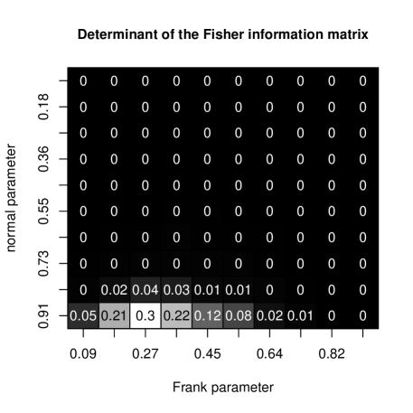
Figure 1: The determinant of the Fisher information matrix for case study 5.

As one can see, the model is locally identifiable in a narrow part of the space of the parameters, picking at around (0.91, 0.27).

4 Data generation

To generate one realization $(u_{1},\dots,u_{d})$ of the random vector $(U_{1},\dots,U_{d})$ with distribution $C$ given by (2), one takes the second part of $(u_{0},u_{1},\dots,u_{d})$, from $u_{1}$ to $u_{d}$, a realization of $(U_{0},U_{1},\dots,U_{d})$, where $U_{0}$ is the latent factor. Remembering that, given $U_{0}=u_{0}$, the distribution of $(U_{1},\dots,U_{d})$ can be split into the inner copula $C_{u_{0}}^{\diamond}$ and a set of univariate margins $\{C_{i|0}(u_{i}|u_{0})\}=\{\frac{\partial C_{i}(u_{i},u_{0})}{\partial u_{0}}\}$, with $C_{i|0}^{-1}(\bullet|u_{0})$ denoting the inverse function, $i\in\{1,\dots,d\}$, the following algorithm produces the desired output.

Algorithm 1 Generating one observation from (2).

1:Generate one observation $u_{0}$ from a standard uniform random variable.

2:Generate one observation $(u^{\diamond}_{1},\ldots,u^{\diamond}_{d})$ from $C_{u_{0}}^{\diamond}$.

3:Put $u_{i}=C_{i|0}^{-1}(u^{\diamond}_{i}|u_{0})$ for $i=1,\dots,d$.

Note that, in the presence of conditional invariance, step 1 in the above algorithm is not required for step 2. Needless to say, in the first step, one could have sampled from $F_{0}$, the distribution of $X_{0}$, and in the second step, one would have sampled from $C_{x_{0}}$ instead of $C_{u_{0}}^{\diamond}$.

Data generation for a NEOFC can be performed using a generalized version of Algorithm 1. The main hurdle for this generalization is to define $G_{i}^{-1}$, such that

$$G_{i}^{-1}(G_{i}(u_{i};t_{w},\ldots t_{1});t_{w},\ldots,t_{1})=u_{i},$$

or, in short, such that $G_{i}^{-1}(G_{i}(u_{i}))=u_{i}$.

Recall that

$$G_{i}(u_{i};t_{w},\ldots,t_{1})=H_{iw}^{t_{w}}\circ\dots\circ H_{i1}^{t_{1}}(u_{i})$$

and that $H_{ij}^{t_{j}}(u_{i})=\frac{\partial C_{ij}(u_{i},t_{j})}{\partial t_{j}}$.

Now define $H_{ij}^{-1,t_{j}}$ as the inverse function of $H_{ij}^{t_{j}}$, that is,

$$H_{ij}^{-1,t_{j}}(H_{ij}^{t_{j}}(u_{i}))=u_{i}.$$

This is the same as writing

$$H_{ij}^{-1,t_{j}}\circ H_{ij}^{t_{j}}(u_{i})=u_{i}.$$

Since $G_{i}$ is just a composition of the form $H_{iw}^{t_{w}}\circ\dots\circ H_{i1}^{t_{1}}(u_{i})$, we can extract back $u_{i}$ using the composition $H_{i1}^{-1,t_{1}}\circ\dots\circ H_{iw}^{-1,t_{w}}(\bullet)$. The inverse of $G_{i}$ is therefore:

$$G_{i}^{-1}(\bullet)=H_{i1}^{-1,t_{1}}\circ\dots\circ H_{iw}^{-1,t_{w}}(\bullet).$$ (4.1)

Now that $G_{i}^{-1}$ is defined, Algorithm 2, the generalized version of Algorithm 1, can be given.

Input. A NEOFC, that is, a $d$-variate copula $C_{t_{w}}^{\diamond_{w}}$, the related mappings, $d\times w$ bivariate copulas $\{C_{ij}\}$, and the related parameters.

Output. One observation from the input NEOFC, as a $d$-dimensional vector.

Algorithm 2 Generating one observation from a NEOFC.

1:Generate $w$ observations from a uniform random variable on [0,1]. Denote these values as $t_{1},\ldots,t_{w}$.

2:Generate one observation from $C_{t_{w}}^{\diamond_{w}}$. Denote the resulting vector as $u_{1}^{\diamond_{w}}\ldots u_{d}^{\diamond_{w}}$.

3:On each $u_{i}^{\diamond_{w}}$ in $\{u_{1}^{\diamond_{w}},\ldots,u_{d}^{\diamond_{w}}\}$, run the corresponding function $G_{i}^{-1}(\bullet;t_{w},\ldots,t_{1})$. Denote the result as $u_{i}$.

The end result of the last step of Algorithm 2 is a vector $(u_{1},\ldots,u_{d})$, one observation from the input NEOFC. Run Algorithm 2 multiple times to get multiple observations.

Critical to both algorithms in this section is the inversion of $\frac{\partial C_{i}(u_{i},u_{0})}{\partial u_{0}}$ with respect to $u_{i}$ in the case of an EOFC or of $\frac{\partial C_{ij}(u_{i},t_{j})}{\partial t_{j}}$ with respect to $u_{i}$ in the case of a NEOFC. This is usually not hard to get symbolically. In the worst cases, $C_{i|0}^{-1}$ or $H_{ij}^{-1,t_{j}}$ can be get numerically.

5 Models

In this section, several models built from Equation (2) or Equation (2.11) are presented, including many well-known copula models from the literature.

Krupskii-Huser-Genton copulas.

In their paper, Krupskii et al. (2016) offer a new family of one-factor copulas that can be used to model replicated spatial data. Let $C_{A}$ be a $d$-variate Gaussian copula with correlation matrix $A=\{\rho_{ij}\}$. Let

$$F_{\bullet}(x_{i})=\int_{-\infty}^{+\infty}\Phi(x_{i}-x_{0})dF_{0}(x_{0}),$$

where $F_{0}$ is some univariate CDF, while $\Phi$ is the CDF of the univariate standard Gaussian distribution. Then, the KHG family of copulas corresponds to an EOFC where $C_{Q_{0}(u_{0})}^{\diamond}=C^{\diamond}=C_{A}$ and $\frac{\partial C_{i}(u_{i},u_{0})}{\partial u_{0}}=\Phi(F_{\bullet}^{-1}(u_{i})-F_{0}^{-1}(u_{0}))$, $\forall i\in\{1,\ldots d\}$.

As shown by Krupskii et al. (2016), tail dependence and tail asymmetry for this model is possible, based on the choice of $F_{0}$ and $A$.

Let $C^{[i,j]}(u_{i},u_{j})$, $i\neq j$, be a bivariate margin of $C$, the outer copula. Recall that the lower tail dependence of a bivariate copula, such as $C^{[i,j]}(u_{i},u_{j})$, is (Hartmann et al., 2004; McNeil et al., 2015):

$$\lambda^{L}_{ij}=\lim_{q\rightarrow 0}\frac{C^{[i,j]}(q,q)}{q},$$

while the upper one is defined as

$$\lambda^{U}_{ij}=\lim_{q\rightarrow 0}\frac{2q-1+C^{[i,j]}(1-q,1-q)}{q}.$$

As an example, if

$$F_{0}(x_{0})=1-Kx_{0}^{\beta}e^{-\theta x_{0}^{\alpha}},$$

Krupskii et al. (2016) showed that for any bivariate margin $C^{[i,j]}(u_{i},u_{j})$ of $C$, as long as $\theta,K>0$, $0<\alpha<1$ and $\beta\in\mathbb{R}$, or as long as $\theta,K>0$, $\alpha=0$ and $\beta<0$,

$$\lambda^{U}_{ij}=1.$$

A more interesting case however arises if $\theta,K>0$, $\alpha=1$ and $\beta\in\mathbb{R}$. Then,

$$\lambda^{U}_{ij}=2\Phi\bigg{[}-\theta\sqrt{\frac{1-\rho_{ij}}{2}}\bigg{]},$$

meaning that tail asymmetry becomes possible through the correlation matrix $A=\{\rho_{ij}\}$.

The upper tail dependence coefficient can also be made such that $\lambda^{U}_{ij}=0$: one need to let $\theta,K>0$, $\alpha>1$ and $\beta\in\mathbb{R}$.

For more examples and details, refer to Krupskii et al. (2016).

Farlie-Gumbel-Morgenstern copulas.

Let the inner copula of a bidimensional EOFC be such that $C^{\diamond}_{Q_{0}(u_{0})}=\Pi$, while $C_{1},C_{2}$ are Farlie-Gumbel-Morgenstern copulas with parameters $\theta_{1}$ and $\theta_{2}$. Then, the resulting outer copula is a FGM copula with parameter $\frac{\theta_{1}\theta_{2}}{3}$. Although a bit tedious, the proof is trivial. Also refer to Example 3.16.

Note that in a bivariate FGM with parameter $\theta\in[-1,1]$, the related Kendall’s tau is $\tau=\frac{2\theta}{9}$ (Nelsen, 2006, p. 162). This means that even if the parameters $\theta_{1}$ and $\theta_{2}$ of $C_{1}$ and $C_{2}$ are set to their upper limit, the parameter of the resulting FGM will be 1/3, corresponding to a rather low Kendall’s tau of 0.074. The model where $C^{\diamond}_{Q_{0}(u_{0})}=\Pi$, while $C_{1},C_{2}$ are FGM copulas, is thus trapped between a correlation of -0.074 and 0.074 only. This can be fixed using EOFCs.

In an EOFC, the inner copula can be viewed as the baseline level of dependence. Instead of letting $C^{\diamond}_{Q_{0}(u_{0})}=\Pi$, one could let $C^{\diamond}_{Q_{0}(u_{0})}=M$, where $M$ is the upper Fréchet-Hoeffding bound. In this scheme, the two FGM copulas $C_{1},C_{2}$ can only be used to decrease the dependence between the two random variables of interest, $U_{1}$ and $U_{2}$. Figure 2 shows the empirical Kendall’s tau calculated (sample size = 1000) for various combinations of $\theta_{1}$ and $\theta_{2}$ when the inner copula is $M$. As one can see, the improved model is now trapped between a correlation of $\sim 0.55$ and 1. This range can thus be tuned by changing the inner copula.

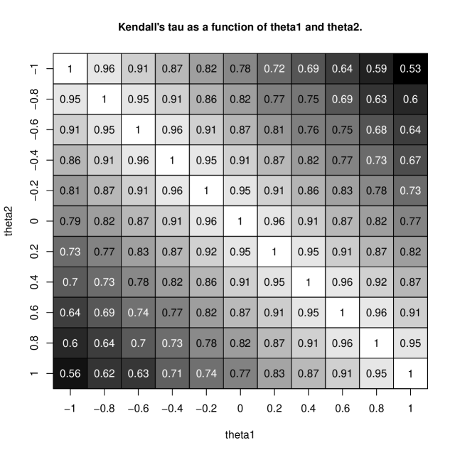
Figure 2: Empirical Kendall’s tau for an EOFC where the inner copula is $M$ and $C_{1},C_{2}$ are FGM copulas, described through $\theta_{1}\in[-1,1]$ and $\theta_{2}\in[-1,1]$.

Archimedean copulas.

Let $\psi$ be a completely monotonic function on $[0,\infty]$, that is, $(-1)^{k}d^{k}/dt^{k}\psi(t)\geqslant 0$ for all integers $k$ and all $t>0$, and such that $\psi(0)=1$ while

$$\psi(\infty)=\lim_{t\to\infty}\psi(t)=0.$$

If a copula $C$ can be written as

$$C(u_{1},\dots,u_{d})=\psi(\psi^{-1}(u_{1})+\dots+\psi^{-1}(u_{d})),$$

then it is called an Archimedean copula with generator $\psi$ (McNeil, 2008). Let us note that, in order to make sure $C$ is a proper copula, the above-mentioned conditions on $\psi$ are sufficient, but not necessary. For sufficient and necessary conditions, see McNeil and Nešlehová (2009).

Proposition 5.1.

In (2), let $C_{x_{0}}=\Pi$, assume that the support of $X_{0}$ is $[0,\infty]$, and put

$$C_{i}(u_{i},u_{0})=\int_{0}^{Q_{0}(u_{0})}e^{-t\psi^{-1}(u_{i})}f_{0}(t)\,dt,$$

where

$$\psi(x)=\int_{0}^{\infty}e^{-tx}f_{0}(t)\,dt,$$

$i\in\{1,\dots,d\}$, with $f_{0}$ being the derivative of $F_{0}$ and $Q_{0}$ its inverse, with $Q_{0}(u_{0})=x_{0}$. It can be checked that $\psi$ is completely monotonic, see for instance Joe (2001). Then $C$, the left-hand side of equation (2), is an Archimedean copula with generator $\psi$.

Proof.

Checking that $C_{i}$ is a copula is straightforward. Moreover, since

$$\frac{\partial C_{i}(u_{i},u_{0})}{\partial u_{0}}=e^{-Q_{0}(u_{0})\psi^{-1}(u_{i})},$$

it holds that

$$C(u_{1},\dots,u_{d})=\int_{0}^{\infty}e^{-x_{0}\,\sum_{i=1}^{d}\psi^{-1}(u_{i})}f_{0}(x_{0})\,dx_{0}=\psi\Big{(}\sum_{i=1}^{d}\psi^{-1}(u_{i})\Big{)}.$$

∎

Note that a reformulation of the above construction can be found in Joe (2001).

Hierarchical Archimedean copulas.

Archimedean copulas can be nested in order to get more flexible models. Hierarchical or Nested Archimedean copulas (HACs or NACs) were introduced by Joe (2001) and have been the main topic of many research papers since, see for instance McNeil (2008), Hofert and Pham (2013), or Okhrin et al. (2013). The simplest hiearchical Archimedean copula consists of a bivariate Archimedean copula

$$C_{12}(u_{1},u_{2})=\psi_{12}(\psi^{-1}_{12}(u_{1})+\psi^{-1}_{12}(u_{2})),$$

which is nested into another bivariate Archimedean copula

$$C_{123}(\bullet,u_{3})=\psi_{123}(\psi^{-1}_{123}(\bullet)+\psi^{-1}_{123}(u_{3}))$$

in order to get a copula of the form

$$C(u_{1},u_{2},u_{3})=C_{123}(C_{12}(u_{1},u_{2}),u_{3})\\ =\psi_{123}\big{(}\psi_{123}^{-1}(\psi_{12}(\psi_{12}^{-1}(u_{1})+\psi_{12}^{-1}(u_{2})))+\psi_{123}^{-1}(u_{3})\big{)}.$$ (5.1)

In general, an arbitrary pair of generators $(\psi_{123},\psi_{12})$ does not ensure that the copula in Equation (5.1) is a proper copula. See Joe (2001) and McNeil (2008) for more on this matter.

Proposition 5.2.

Define $\psi_{123}$ the same way $\psi$ was defined in Proposition 5.1. Also let $C_{i}$ as in Proposition 5.1. Further define

$$C_{x_{0}}(u,v,w)=\exp\Bigg{(}-x_{0}\times\nu\bigg{(}\nu^{-1}\Big{[}\frac{1}{x_{0}}\log\Big{(}\frac{1}{u}\Big{)}\Big{]}+\nu^{-1}\Big{[}\frac{1}{x_{0}}\log\Big{(}\frac{1}{v}\Big{)}\Big{]}\bigg{)}\Bigg{)}\times w;$$

where $\nu(\bullet)=\psi_{123}^{-1}\big{(}\psi_{12}(\bullet)\big{)}$, $\nu(\bullet)^{-1}=\psi_{12}^{-1}\big{(}\psi_{123}(\bullet)\big{)}$ and $\psi_{12}(\bullet)$ is equal to the integral from $0$ to $\infty$ of $\exp(-t\bullet)dF_{12}(t)$ with $F_{12}$ some distribution function. Then (2) is the copula given in (5.1).

Proof.

First, it is proven that $C_{x_{0}}$ is a copula. Define, for $0\leq u,v,w\leq 1$,

$$G_{x_{0}}(u,v,w)=\exp\Bigg{(}-x_{0}\times\nu\bigg{(}\nu^{-1}\Big{[}\psi_{123}^{-1}\Big{(}u\Big{)}\Big{]}+\nu^{-1}\Big{[}\psi_{123}^{-1}\Big{(}v\Big{)}\Big{]}\bigg{)}\Bigg{)}\\ \times\exp\Bigg{(}-x_{0}\times\psi_{123}^{-1}\bigg{(}w\bigg{)}\Bigg{)}.$$

One can check that $C_{x_{0}}$ in Proposition 5.2 is the copula corresponding to the multivariate distribution $G_{x_{0}}$. And from Joe (2001), page 88, it can be easily deduced that $G_{x_{0}}$ is indeed a distribution function. Therefore $C_{x_{0}}$ is a proper copula.

The proof then proceeds by showing that $C$ in (2) is a hierarchical Archimedean copula. $C$ in (2) becomes

$$C(u_{1},u_{2},u_{3})=\int_{0}^{1} \exp\Bigg{(}-Q_{0}(u_{0})\times\nu\bigg{(}\nu^{-1}\Big{[}\frac{1}{Q_{0}(u_{0})}\log\Big{(}\frac{1}{C_{1|0}(u_{1}|u_{0})}\Big{)}\Big{]}$$ (5.2)

$$+\nu^{-1}\Big{[}\frac{1}{Q_{0}(u_{0})}\log\Big{(}\frac{1}{C_{2|0}(u_{2}|u_{0})}\Big{)}\Big{]}\bigg{)}\Bigg{)}\times C_{3|0}(u_{3}|u_{0})\,du_{0}.$$

In the proof of Proposition 5.1, it was shown that $\frac{\partial C_{i}(u_{i},u_{0})}{\partial u_{0}}=C_{i|0}(u_{i}|u_{0})=\exp(-Q_{0}(u_{0})\times\psi_{123}^{-1}(u_{i}))$. Replacing in (5.2) gives

$$\int_{0}^{1}\exp\Bigg{(}-Q_{0}(u_{0})\times\nu\bigg{(}\nu^{-1}\Big{[}\psi_{123}^{-1}(u_{1})\Big{]}+\nu^{-1}\Big{[}\psi_{123}^{-1}(u_{2})\Big{]}\bigg{)}\Bigg{)}$$

$$\qquad\qquad\qquad\qquad\qquad\qquad\qquad\qquad\qquad\qquad\exp(-F_{0}^{-1}(u_{0})\times\psi_{123}^{-1}(u_{3}))\,du_{0}$$

$$= \int_{0}^{\infty}\exp\Bigg{(}-x_{0}\bigg{[}\psi_{123}^{-1}\bigg{(}\psi_{12}\Big{(}\psi_{12}^{-1}(u_{1})+\psi_{12}^{-1}(u_{2})\Big{)}\bigg{)}+\psi_{123}^{-1}(u_{3})\bigg{]}\Bigg{)}dF_{0}(x_{0})$$

$$= \,\,\psi_{123}\big{(}\psi_{123}^{-1}(\psi_{12}(\psi_{12}^{-1}(u_{1})+\psi_{12}^{-1}(u_{2})))+\psi_{123}^{-1}(u_{3})\big{)},$$

which is the NAC from (5.1). ∎

Hierarchical NEOFCs.

OFCs are not suited to model hierarchical dependence. Assume that one wishes to build a one-factor copula on $(U_{1},U_{2},U_{3},U_{4})$ such that the resulting model is described by the matrix of Kendall’s taus in (5.3).

$$\begin{matrix}&U_{1}&U_{2}&U_{3}&U_{4}\\ U_{1}&&1&0.25&0.25\\ U_{2}&&&0.25&0.25\\ U_{3}&&&&1\\ U_{4}&&&&\end{matrix}$$ (5.3)

Since $U_{1}$ and $U_{2}$ are related through the maximum value of 1, it means that their bivariate margin must be

$$C^{[1,2]}(u_{1},u_{2})=\min(u_{1},u_{2})=\int_{0}^{1}\frac{\partial\min(u_{1},u_{0})}{\partial u_{0}}\frac{\partial\min(u_{2},u_{0})}{\partial u_{0}}du_{0}.$$

Similarly, the bivariate margin of $U_{3}$ and $U_{4}$ is

$$C^{[3,4]}(u_{3},u_{4})=\min(u_{3},u_{4})=\int_{0}^{1}\frac{\partial\min(u_{3},u_{0})}{\partial u_{0}}\frac{\partial\min(u_{4},u_{0})}{\partial u_{0}}du_{0}.$$

Therefore, the OFC on $(U_{1},U_{2},U_{3},U_{4})$ has to be

$$C(u_{1},u_{2},u_{3},u_{4})=\int_{0}^{1}\frac{\partial\min(u_{1},u_{0})}{\partial u_{0}}\frac{\partial\min(u_{2},u_{0})}{\partial u_{0}}\frac{\partial\min(u_{3},u_{0})}{\partial u_{0}}\frac{\partial\min(u_{4},u_{0})}{\partial u_{0}}du_{0}.$$

By proposition 3.3 however, this corresponds to $C(u_{1},u_{2},u_{3},u_{4})=\min(u_{1},\allowbreak u_{2},u_{3},u_{4})$, for which the correlation matrix is not (5.3). A OFC will never be able to reproduce a matrix of Kendall’s taus such as the one in (5.3). In general, OFCs do not seem to be suited to model matrices of the form

$$\begin{matrix}&U_{1}&U_{2}&U_{3}&U_{4}\\ U_{1}&&\tau_{12}&\tau_{0}&\tau_{0}\\ U_{2}&&&\tau_{0}&\tau_{0}\\ U_{3}&&&&\tau_{34}\\ U_{4}&&&&\end{matrix}$$ (5.4)

in which $\tau_{12},\tau_{34}>\tau_{0}$.

On the other hand, it is possible to build NEOFCs for which the matrix of Kendall’s taus is as in (5.4).

Start from Equation (2.11), and let $w=3$, that is, we have a triple layer of linking copulas. Let $C_{t_{3}}^{\diamond_{3}}=\Pi$. For $j=3$, let all linking copulas $C_{ij}$ be a Frank copula with a same parameter $\theta_{3}$. This layer gives the baseline level of dependence between the four random variables of interest. Next, use the second layer, $j=2$, to couple $U_{1}$ and $U_{2}$, that is, let $C_{12}$ and $C_{22}$ be a Frank copula with a common paramater $\theta_{2}$, while $C_{32}$ and $C_{42}$ are set to the independence copula. Finally use the first layer, $j=1$, to couple $U_{3}$ and $U_{4}$, that is, let $C_{31}$ and $C_{41}$ be a Frank copula with a common paramater $\theta_{1}$, while $C_{11}$ and $C_{21}$ are set to the independence copula. Table 4 allows one to visualize this scheme.

	$i=1$	$i=2$	$i=3$	$i=4$
$j=1$	$\Pi$	$\Pi$	Frank	Frank	$\theta_{1}$
$j=2$	Frank	Frank	$\Pi$	$\Pi$	$\theta_{2}$
$j=3$	Frank	Frank	Frank	Frank	$\theta_{3}$
$C^{\diamond}$	$\Pi$

Table 4: A hierarchical NEOFC with three layers and an inner copula set to independence.

Example 5.3.

In Table 4, set $\theta_{3}$ to a value of 5.74, corresponding to a Kendall’tau of 0.5 for the related linking copulas and $\theta_{2}=\theta_{1}$ to a value of 6.73, corresponding to a Kendall’s tau of 0.55 for the related linking copulas. The empirical Kendall’s taus based on 10000 observations generated from the model through Algorithm 2 are as shown hereafter.

> round(cor(generated.data, method="kendall"), 3)
      [,1]  [,2]  [,3]  [,4]
[1,] 1.000 0.559 0.119 0.123
[2,] 0.559 1.000 0.118 0.121
[3,] 0.119 0.118 1.000 0.563
[4,] 0.123 0.121 0.563 1.000

While the correlation between $U_{1}$, $U_{2}$ and $U_{3}$, $U_{4}$ is strong, one can note that even though $\theta_{3}$ corresponds to a correlation of 0.5, the correlation for the couples $(U_{1},U_{3})$, $(U_{1},U_{4})$, $(U_{2},U_{3})$ and $(U_{2},U_{4})$ appears to have dampen to $\sim 0.12$. Pushing $\theta_{3}$ towards higher values can help: if $\theta_{3}$ is set to a value of 14.14, corresponding to a Kendall’s tau of 0.75, the empirical Kendall’s taus become as shown hereafter.

> round(cor(generated.data, method="kendall"), 3)
      [,1]  [,2]  [,3]  [,4]
[1,] 1.000 0.743 0.220 0.222
[2,] 0.743 1.000 0.219 0.222
[3,] 0.220 0.219 1.000 0.738
[4,] 0.222 0.222 0.738 1.000

This increase remains however slow and even with a high value for $\theta_{3}$, such as 38.28, corresponding to a Kendall’s tau of 0.9, the correlation between $U_{1}$ and $U_{3}$ will not exceed 0.27.

To overcome the issue of low dependence between the pairs $(U_{1},U_{3})$, $(U_{1},U_{4})$, $(U_{2},U_{3})$ and $(U_{2},U_{4})$, one can make use of the inner copula to set the baseline level of dependence, rather than using a layer of identical linking copulas. See Table 5.

	$i=1$	$i=2$	$i=3$	$i=4$
$j=1$	$\Pi$	$\Pi$	Frank	Frank	$\theta_{1}$
$j=2$	Frank	Frank	$\Pi$	$\Pi$	$\theta_{2}$
$C^{\diamond}$	Frank				$\theta^{\diamond}$

Table 5: A hierarchical NEOFC with 2 layers and an inner copula set to a Frank copula.

Example 5.4.

In Table 5, set $\theta^{\diamond}$ to a value of 14.14, corresponding to a Kendall’s $\tau$ of 0.75, $\theta_{2}$ to 1.38, corresponding to a Kendall’s tau of 0.15, and $\theta_{1}$ to 6.73, corresponding to a Kendall’s $\tau$ of 0.55. The empirical Kendall’s taus based on 10000 observations generated from the related hierarchical NEOFC are shown hereafter.

> round(cor(generated.data, method="kendall"), 3)
      [,1]  [,2]  [,3]  [,4]
[1,] 1.000 0.755 0.388 0.385
[2,] 0.755 1.000 0.387 0.385
[3,] 0.388 0.387 1.000 0.809
[4,] 0.385 0.385 0.809 1.000

As last example of a hierarchical NEOFC, we revisit the tree on the right of Figure 11 in Segers and Uyttendaele (2014), this tree corresponding to an attempt to map the dependencies between daily log returns using hierarchical Archimedean copulas. Figure 11 in Segers and Uyttendaele (2014) is, for convenience, reproduced in this paper as Figure 3.

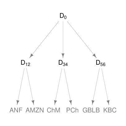
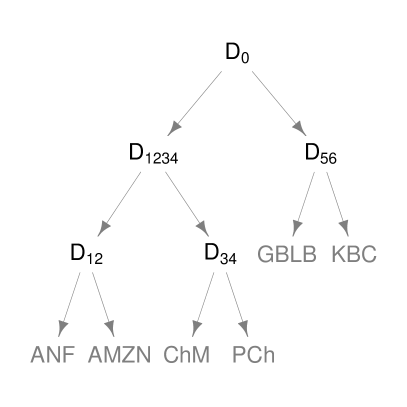
Figure 3: Figure 11 in Segers and Uyttendaele (2014).

The tree on the right of Figure 3 corresponds to the hierarchical NEOFC from Table 6, where the symbols $\{\text{D}_{0},\text{D}_{1234},\text{D}_{56},\text{D}_{12},\text{D}_{34}\}$ on the right of the table are there to help one compare the table with the tree on the right of Figure 3.

	$i=1$	$i=2$	$i=3$	$i=4$	$i=5$	$i=6$
$j=1$	$\Pi$	$\Pi$	Frank	Frank	$\Pi$	$\Pi$	$\text{D}_{34}$
$j=2$	Frank	Frank	$\Pi$	$\Pi$	$\Pi$	$\Pi$	$\text{D}_{12}$
$j=3$	$\Pi$	$\Pi$	$\Pi$	$\Pi$	Frank	Frank	$\text{D}_{56}$
$j=4$	Frank	Frank	Frank	Frank	$\Pi$	$\Pi$	$\text{D}_{1234}$
$C^{\diamond}$	Frank						$\text{D}_{0}$

Table 6: The hierarchical NEOFC corresponding to the tree structure on the right of Figure 3.

Note that, given the tree structure of a hierarchical Archimedean copula, the corresponding NEOFC will have as many layers as there are internal nodes in the tree when the inner copula is set to independence, or, when the inner copula is used as root node, as many layers as there are internal nodes in the tree minus one.

Example 5.5.

Set the various parameters of Table 6 to the arbitrary values shown in Table 7. The empirical Kendall’s taus based on 10000 observations generated from the related hierarchical NEOFC are shown hereafter.

> round(cor(generated.data, method="kendall"), 3)
      [,1]  [,2]  [,3]  [,4]  [,5]  [,6]
[1,] 1.000 0.776 0.400 0.406 0.476 0.478
[2,] 0.776 1.000 0.404 0.407 0.475 0.475
[3,] 0.400 0.404 1.000 0.775 0.485 0.483
[4,] 0.406 0.407 0.775 1.000 0.489 0.487
[5,] 0.476 0.475 0.485 0.489 1.000 0.755
[6,] 0.478 0.475 0.483 0.487 0.755 1.000

Note that, in contrast to what is usually required for hierarchical Archimedean copulas, the dependence in hierarchical NEOFCs is not required to be a nondecreasing function as one goes farther away from the root node. The empirical matrix from the last example indeed shows that the dependence at node $D_{12}$ is $\sim 0.776$, that of node $D_{1234}=D_{1:4}$ is lower, around $0.400$, but that of the root is higher than $0.400$, at around 0.475.

	$i=1$	$i=2$	$i=3$	$i=4$	$i=5$	$i=6$
$j=1$	$\Pi$	$\Pi$	$\tau_{34}=0.4$	$\tau_{34}=0.4$	$\Pi$	$\Pi$	$D_{34}$
$j=2$	$\tau_{12}=0.4$	$\tau_{12}=0.4$	$\Pi$	$\Pi$	$\Pi$	$\Pi$	$D_{12}$
$j=3$	$\Pi$	$\Pi$	$\Pi$	$\Pi$	$\tau_{56}=0.2$	$\tau_{56}=0.2$	$D_{56}$
$j=4$	$\tau_{1234}=0.1$	$\tau_{1234}=0.1$	$\tau_{1234}=0.1$	$\tau_{1234}=0.1$	$\Pi$	$\Pi$	$D_{1:4}$
$C^{\diamond}$	$\tau_{0}=0.75$						$D_{0}$

Table 7: Parameters for Example 5.5, expressed as Kendall’s taus for convenience.

Gaussian copulas.

A Gaussian copula is a copula whose density $c$ satisfies

$$\log(c(u_{1},\dots,u_{d}))=-\frac{1}{2}\log(\text{det}(R))-\frac{1}{2}z^{\top}(R^{-1}-I)z,$$ (5.5)

where $R$ is a $d\times d$ invertible correlation matrix, $z=(z_{1},\dots,z_{d})^{\top}$ and $z_{i}$ is the quantile of order $u_{i}$ of the standard normal distribution. A Gaussian copula can be represented as in (2). Let $\Delta=(\Delta_{1},\dots,\Delta_{d})^{\top}$ be a real vector in $[0,1]^{d}$ and let $D$ be a diagonal matrix with elements given by $1-\Delta_{i}^{2},\,i=1,\dots,d$. Finally let $C_{A}$ be a $d$-variate Gaussian copula with correlation matrix $A$.

Proposition 5.6.

Let $C^{\diamond}_{Q_{0}(u_{0})}=C^{\diamond}=C_{A}$ and let $C_{i}$ be a bivariate Gaussian copula with correlation $\Delta_{i}$, $i\in\{1,\dots,d\}$. Then the outer copula in (2) is a Gaussian copula with correlation matrix given by $R=D^{1/2}AD^{1/2}+\Delta\Delta^{T}$.

Proof.

Let $R$ be a symmetric nonnegative matrix whose diagonal elements are equal to $1$ and whose element in the $i$-th row and $j$-th column is denoted $\Delta_{ij}$. Let $(Z_{1},\dots,Z_{d},Z_{0})$ be distributed according to a $(d+1)$-variate centered Gaussian distribution with variance-covariance matrix given by

$$\begin{pmatrix}\underset{d\times d}{R}&\underset{d\times 1}{\Delta}\\ \underset{1\times d}{\Delta^{T}}&\underset{1\times 1}{1}\end{pmatrix},$$

so that $(Z_{1},\dots,Z_{d}|Z_{0}=z_{0})\sim N(\Delta z_{0},\,R-\Delta\Delta^{\top})$. The partial correlations are given by

$$\text{Cov}(Z_{i},Z_{j}|Z_{0}=z_{0})=\text{Corr}(Z_{i},Z_{j}|Z_{0}=z_{0})=\frac{\Delta_{ij}-\Delta_{i}\Delta_{j}}{\sqrt{(1-\Delta_{i}^{2})(1-\Delta_{j}^{2})}},$$

or, in other words, the partial correlation matrix is $A=D^{-1/2}(R-\Delta\Delta^{\top})D^{-1/2}$. Given $Z_{0}=z_{0}$, the margins $(Z_{i}|Z_{0}=z_{0})$ are $N(\Delta_{i}z_{0},1-\Delta_{i}^{2})$, hence

$$P(Z_{i}\leq z|Z_{0}=z_{0})=\Phi((z-\Delta_{i}z_{0})/\sqrt{1-\Delta_{i}^{2}}),$$

and, moreover, the corresponding copula is a Gaussian copula $C_{A}$, with correlation matrix $A$.

Calculate the copula corresponding to $(Z_{1},\dots,Z_{d})$. Let $\Phi$ be the cumulative distribution function of the univariate standard Gaussian distribution.

$$C_{(Z_{1},\dots,Z_{d})}(u_{1},\dots,u_{d})$$

$$= \int P(\Phi(Z_{i})\leq u_{i},\,i=1,\dots,d|Z_{0}=z_{0})\Phi^{\prime}(z_{0})dz_{0}$$

$$= \int P(Z_{i}\leq\Phi^{-1}(u_{i}),\,i=1,\dots,d|Z_{0}=z_{0})\Phi^{\prime}(z_{0})dz_{0}$$

$$= \int C_{A}\left\{\Phi\left(\frac{\Phi^{-1}(u_{i})-\Delta_{i}z_{0}}{\sqrt{1-\Delta_{i}^{2}}}\right),i=1,\dots,d\right\}\Phi^{\prime}(z_{0})dz_{0}$$

$$= \int_{0}^{1}C_{A}\left\{\Phi\left(\frac{\Phi^{-1}(u_{i})-\Delta_{i}\Phi^{-1}(u_{0})}{\sqrt{1-\Delta_{i}^{2}}}\right),i=1,\dots,d\right\}du_{0}.$$

This expression corresponds exactly to the copula given in (2), with

$$\frac{\partial C_{i}(u_{i},u_{0})}{\partial u_{0}}=\Phi\left(\frac{\Phi^{-1}(u_{i})-\Delta_{i}\Phi^{-1}(u_{0})}{\sqrt{1-\Delta_{i}^{2}}}\right),$$

see Meyer (2013) for details.

∎

Note: in the case $d=2$, the outer copula is a Gaussian copula with correlation given by

$$\rho_{A}\sqrt{1-\Delta_{1}^{2}}\sqrt{1-\Delta_{2}^{2}}+\Delta_{1}\Delta_{2}.$$

Also see Example 3.18.

C-Vine copulas.

Let $(U_{0},U_{1},\dots,U_{d})$ be a random vector following a C-Vine copula distribution truncated after the second level. The density of this truncated C-Vine is given by

$$c(u_{0},\dots,u_{d})=\prod_{i=1}^{d-1}c^{*}_{1,1+i|0}(C^{*}_{1|0}(u_{1}|u_{0}),C^{*}_{1+i|0}(u_{1+i}|u_{0})|u_{0})\prod_{i=1}^{d}c_{i}^{*}(u_{i},u_{0})$$ (5.6)

where $c^{*}_{i}=\partial^{2}C^{*}_{i}(u_{i},u_{0})/\partial u_{i}\partial u_{0}$, $C^{*}_{i|0}(u_{i}|u_{0})=\partial C^{*}_{i}(u_{i},u_{0})/\partial u_{0}$, $\{C^{*}_{i}(u_{i},u_{0})\}$ is a set of $d$ arbitrary bivariate copulas, and $\{c^{*}_{1,1+i|0}\}$ is a set of $d-1$ abritrary copula densities for each $u_{0}$. Due to their extreme flexibility and ease of use (one only has to specify sets of bivariate copulas), Vine copulas have been used in an increasing number of applications and are still a hot topic of research, see for instance Aas et al. (2009), Kurowicka and Joe (2011) or Bedford and Cooke (2002).

Proposition 5.7.

If, in (3.6), where $T_{1}=U_{0}$ and $t_{1}=u_{0}$, for each $u_{0}$, $c_{u_{0}}$ is defined as

$$c_{u_{0}}(u_{1},\dots,u_{d})=\prod_{i=1}^{d-1}c^{*}_{1,1+i|0}(u_{1},u_{1+i}|u_{0}),$$

and $c_{i}(u_{i},u_{0})=c_{i}^{*}(u_{i},u_{0})$ for all $i$, then the outer copula $c$ in (3.6) is the $d$-variate marginal distribution, with respect to $u_{0}$, of (5.6), that is, its density is

$$c(u_{1},\dots,u_{d})= \int_{0}^{1}c_{u_{0}}(C^{*}_{1|0}(u_{1}|u_{0}),\dots,C^{*}_{d|0}(u_{d}|u_{0}))\,\prod_{i=1}^{d}c^{*}_{i}(u_{i},u_{0})du_{0}$$

$$= \int_{0}^{1}\prod_{i=1}^{d-1}c^{*}_{1,1+i|0}(C^{*}_{1|0}(u_{1}|u_{0}),C^{*}_{1+i|0}(u_{1+i}|u_{0})|u_{0})\prod_{i=1}^{d}c^{*}_{i}(u_{i},u_{0})\,du_{0}.$$

If one assumes that, in (5.6), none of the elements of $\{c^{*}_{1,1+i|0}\}$ actually depends on $u_{0}$, then the inner copula in Proposition 5.7 becomes

$$c_{u_{0}}(u_{1},\dots,u_{d})=\prod_{i=1}^{d-1}c^{*}_{1,1+i}(u_{1},u_{1+i}),$$

which is nothing more than a C-Vine on $(U_{1},\ldots,U_{d})$, truncated at the first level.

$p$-factor models.

Define respectively $\Pi_{1}$-factor and $\Pi_{2}$-factor copulas as copulas of the form

$$C^{(\Pi_{1})}(u_{1},\dots,u_{d})=\int_{0}^{1}\prod_{i=1}^{d}C_{i|0}^{(2)}(u_{i}|v_{2})\,dv_{2},\text{ and}$$ (5.7)

$$C^{(\Pi_{2})}(u_{1},\dots,u_{d})=\int_{0}^{1}\int_{0}^{1}\prod_{i=1}^{d}C_{i|0}^{(2)}(C_{i|0}^{(1)}(u_{i}|v_{1})|v_{2})\,dv_{2}\,dv_{1},$$ (5.8)

where $C_{i|0}^{(k)}(u_{i}|v_{k})=\partial C_{i}^{(k)}(u_{i},v_{k})/\partial v_{k}$ for $k=1,2$ and $i=1,\dots,d$, and where the $C_{i}^{(k)}$ are (arbitrary) bivariate copulas. $\Pi_{1}$-factor and $\Pi_{2}$-factor copulas have been studied in Krupskii and Joe (2013, 2015) as copula models for conditionally independent variables given respectively one and two latent factors.

The following (trivial) proposition aims at recovering $\Pi_{1}$-factor and $\Pi_{2}$-factor copulas as special cases of the model (2).

Proposition 5.8.

Consider the copulas given in (5.7) and (5.8). In (2), put $C_{i}=C_{i}^{(2)}$. If, moreover, $C^{\diamond}_{Q_{0}(u_{0})}=\Pi$ for each $u_{0}$, then the outer copula $C$ in (2) is the $\Pi_{1}$-factor copula given in (5.7). Likewise, if, in (2), $C_{i}=C_{i}^{(1)}$ and moreover,

$$C^{\diamond}_{Q_{0}(u_{0})}(u_{1},\dots,u_{d})=\int_{0}^{1}\prod_{i=1}^{d}C_{i|0}^{(2)}(u_{i}|\tilde{u}_{0})\,d\tilde{u}_{0},$$

then the outer copula $C$ in (2) is the $\Pi_{2}$-factor copula given in (5.8).

Note that $C^{\diamond}_{Q_{0}(u_{0})}$ in the above proposition actually does not depend on $u_{0}$ hence we have conditional invariance. This restriction can be easily removed as follows. Let, for each $u_{0}$, $\{\widetilde{C}_{i}(\bullet,\bullet;u_{0})\}$ be a set of bivariate copulas and

$$C^{\diamond}_{Q_{0}(u_{0})}(u_{1},\dots,u_{d})=\int_{0}^{1}\prod_{i=1}^{d}\widetilde{C}_{i|0}(u_{i}|\tilde{u}_{0};u_{0})\,d\tilde{u}_{0},$$

where $\widetilde{C}_{i|0}(u_{i}|\tilde{u}_{0};u_{0})=\partial\widetilde{C}_{i}(u_{i},\tilde{u}_{0};u_{0})/\partial\tilde{u}_{0}$. The outer copula is then

$$C(u_{1},\dots,u_{d})=\int_{0}^{1}\int_{0}^{1}\prod_{i=1}^{d}\widetilde{C}_{i|0}(C_{i|0}(u_{i}|u_{0})|\tilde{u}_{0};u_{0})\,d\tilde{u}_{0}\,du_{0}.$$

6 Inference

This section discusses estimation of models of the form (2) or (2.11), as well as how one can test for conditional independence for models of the form (2).

6.1 Estimation

Let, in (2), $C_{i}(u_{i},u_{0})=C_{i}(u_{i},u_{0};\alpha_{i})$ and

$$C_{x_{0}}(u_{1},\dots,u_{d})=C_{x_{0}}(u_{1},\dots,u_{d};\beta(x_{0})),$$

where $\beta$ is a mapping which, to each $x_{0}$ in the support of $X_{0}$, associates a parameter in the appropriate parameter space. If the mapping $\beta$ depends on a vector of parameters, as in (3.2), we also denote this vector by $\beta$. Likewise, we denote the parameter vector which contains the parameters of the quantile function $Q_{0}$ of $X_{0}$ by $\lambda$. Accordingly, the notation for the copula of $(U_{1},\dots,U_{d}|U_{0}=u_{0})$ becomes $C^{\diamond}_{Q_{0}(u_{0})}(u_{1},\dots,u_{d})=C^{\diamond}(u_{1},\dots,u_{d};\beta,\lambda)$. Finally, let us denote by $(x_{h1},\dots,x_{hd})$, $h=1,\dots,n$, the sample of the distribution $F$ with margins $F_{1},\dots,F_{d}$ and copula $C$.

The pseudo log likelihood function to maximize is

$$L_{n}(\boldsymbol{\theta})=\sum_{h=1}^{n}\log\int_{0}^{1}c\left[C_{1|0}(\widehat{F}_{1}(x_{h1})|u_{0};\alpha_{1}),\dots,C_{d|0}(\widehat{F}_{d}(x_{hd})|u_{0};\alpha_{d});\beta,\lambda\right]\\ \times\prod_{i=1}^{d}c_{i}(\widehat{F}_{i}(x_{hi}),u_{0};\alpha_{i})\,du_{0},$$ (6.1)

where $\boldsymbol{\theta}$ stands for the complete parameter vector, that is, $\boldsymbol{\theta}=(\alpha,\beta,\lambda)$, $\alpha=(\alpha_{1},\dots,\alpha_{d})$ and $\widehat{F}_{i}$ denotes an estimate of $F_{i}$, $i\in\{1,\dots,d\}$. There are many ways to estimate $F_{i}$. For instance, $\widehat{F}_{i}$ may be the empirical distribution function, as in Genest et al. (1995), or may be a parametric estimate, as in Joe and Xu (1996).

Regarding the computational aspects, especially in higher dimensions and for large datasets, the likelihood (6.1) may be costly to compute due to the repeated use of integrals (as many as the sample size). A brief discussion on these computational aspects are given in Section 7.1.

6.2 Testing for conditional independence

This section provides procedures to test for conditional independence in models based on the representation (2). Indeed, being able to assess if the variables of interest are dependent or independent conditioned on the latent factor seems a crucial issue. Conditional independence would mean that the factor captures all the dependence in the data whereas no conditional independence would mean that there is a remaining, intrinsic dependence in the variables even though the factor has been accounted for.

Throughout this subsection, the bivariate copulas $C_{i}$, $i\in\{1,\dots,d\}$, are assumed to belong to some known parametric families. The inner copula $C_{u_{0}}=C^{\diamond}_{Q_{0}(u_{0})}$, however, can be left fully unspecified: either nothing is known about it, either a parametric form is assumed. The possibility to carry out a hypothesis test in this setting is new to the literature.

The hypothesis test for conditional independence is of the form

$$H_{0}:\,C^{\diamond}_{Q_{0}(u_{0})}=\Pi\text{ for all }u_{0}$$

versus $$H_{1}:\text{ there exists some }u_{0}\text{ such that }C^{\diamond}_{Q_{0}(u_{0})}\neq\Pi$$

(recall that $\Pi$ stands for the independence copula or the product function), where for two functions $f$ and $g$, $f=g$ means that $f(t)=g(t)$ for all $t$ in their domain.

If a certain parametric form is assumed for $C^{\diamond}_{Q_{0}(u_{0})}$, such as in Section 2, then most likely the test will reduce to testing for a parameter to equate a certain value, and no conceptual difficulties refrain the task. For instance, in (3.2), testing for conditional independence amounts to testing for $\beta_{0}=\infty$ or $\beta_{1}=\infty$ (conceptually). Let us remark that testing for conditional invariance is also feasible: one need to test $\beta_{1}=0$.

If $C^{\diamond}_{Q_{0}(u_{0})}$ is left fully unspecified, the alternative hypothesis needs to be slightly restricted in order for a test to exist. Consider

$$H_{0}:\,C^{\diamond}_{Q_{0}(u_{0})}=\Pi\text{ for all }u_{0}$$

versus $$H_{1}:\,C^{\diamond}_{Q_{0}(u_{0})}>\Pi\text{ for all }u_{0}.$$ (6.2)

Then, the alternative hypothesis is: “conditioned on the factor, the variables of interest are positively dependent”.

Let $\pi$ be the risk of type I error. One rejects $H_{0}$ if $T_{n}\leq c_{\pi}$, where $c_{\pi}$ is chosen so that $P_{H_{0}}(T_{n}\leq c_{\pi})=\pi$ and where

$$T_{n}=\underset{t\in[0,1]^{d}}{\sup}(M(t)-\widehat{C}(t)),$$ (6.3)

where $M(t)=M(t_{1},\dots,t_{d})=\min(t_{1},\dots,t_{d})$ is the Fréchet-Hoeffding upper bound for copula and

$$\widehat{C}(t)=\frac{1}{n}\sum_{h=1}^{n}\mathbf{1}(\{\widehat{F}_{i}(X_{hi})\leq t_{i}\},\,i=1,\dots,d)$$ (6.4)

is the empirical estimator of $C$ ; $(X_{h1},\dots,X_{hd})$, $h\in\{1,\dots,n\}$, being the data ; and $\widehat{F}_{i}$ being the empirical distribution function of $X_{hi}$.

The heuristic underlying the expression of $T_{n}$, the test statistic, is as follows. Denote by $C^{(H_{0})}$ the outer copula under $H_{0}$, that is, one substitutes $\Pi$ for the inner copula $C^{\diamond}_{Q_{0}(u_{0})}$ in (2) and gets

$$C^{(H_{0})}(u_{1},\dots,u_{d})=\int_{0}^{1}\prod_{i=1}^{d}C_{i|0}(u_{i}|u_{0})\,du_{0}.$$ (6.5)

If $H_{0}$ is true, then the true copula $C$ verifies $C=C^{(H_{0})}$. But if $H_{0}$ is false, $C_{u_{0}}>\Pi$ implies $C>C^{(H_{0})}$. In order to reject the null, one could therefore compare the empirical copula $\widehat{C}$ to $\widehat{C}^{(H_{0})}$, the latter being an estimate of $C^{(H_{0})}$, and reject the null if $\widehat{C}-\widehat{C}^{(H_{0})}$ is too large. However, as the distribution of this difference under $H_{0}$ is unknown, one would need to use bootstrap and fit $C^{(H_{0})}$ to simulated data a large number of times, a process far too expensive for most hardware.

To overcome this issue, the comparison of $\widehat{C}$ to $\widehat{C}^{(H_{0})}$ is done indirectly using the Fréchet-Hoeffding upper bound as a baseline (note that the Fréchet-Hoeffding lower bound for copulas could also be considered as a baseline for comparison, the upper one was however picked since it has the nice property to be a copula $\forall d$, although this property is by no means required for the test). The result of this suggestion is (6.3), which describe a test statistic always positive and expected to take small values when $H_{0}$ is false.

The bootstrap of $T_{n}$ is now described. Note that under $H_{0}$, the outer copula in (6.5) is fully parametric: one can obtain an estimate $\widehat{C}^{(H_{0})}$ by maximum pseudo-likelihood (Krupskii and Joe, 2013). New bootstrap samples (say $N$ of them) are then drawn using Algorithm 1 in order to get $N$ test statistics $T_{n}^{(1)},\dots,T_{n}^{(N)}$. These can be used, for instance, to compute a p-value as $P_{H_{0}}\bigg{(}T_{n}\leq T_{n}^{(obs)}\bigg{)}\approx N^{-1}\sum_{k=1}^{N}\mathbf{1}\bigg{(}T_{n}^{(k)}\leq T_{n}^{(obs)}\bigg{)}$. In other words, the p-value is estimated by counting how many test statistics in $\{T_{n}^{(t)}\},t\in\{1,\ldots,N\}$, are lower or equal than the test statistic $T_{n}^{(obs)}$, built using the data from the original sample.

Finally, let us note that the test $H_{0}:C^{\diamond}_{Q_{0}(u_{0})}=\Pi$ against $H_{1}:C^{\diamond}_{Q_{0}(u_{0})}<\Pi$ can be carried out by considering (6.3) again, but this time with a rejection region on the right, that is, we reject $H_{0}$ if $T_{n}\geqslant c_{\pi}$, where $c_{\pi}$ is chosen so that $P_{H_{0}}(T_{n}\geq c_{\pi})=\pi$.

7 Illustrations

The purpose of this section is to illustrate how one can take advantage of the framework presented in Section 2 in practice and to study the power of the test statistic $T_{n}$ in (6.3) by means of a simulation experiment. We first provide a few technical details on how some numerical operations were performed.

7.1 Computational aspects

In this section, log-likelihoods are maximized using either gradient descent algorithms, which can be found in the optim function of the statistical software R, or differential evolution (Storn and Price, 1997; Qin and Suganthan, 2005; Price et al., 2006), for which a R package also exists: DEoptim (Mullen et al., 2011).

Note that gradient descent algorithms usually require to provide a starting parameter vector. It is advised to try several such points and retain the best result for the likelihood.

For the numerical evaluation of the integral in (6.1), either naive Monte-Carlo integration was used, where the integration space is sampled a thousand times according to a uniform distribution that stretches over the integration space, or adaptative multidimensional integration was used (Steven and Balasubramanian, 2013).

Note that in case of a one-factor copula or of an extended one-factor copula, the integration space is the segment $[0,1]$. However, with a nested extended one-factor copula, the integration space becomes $[0,1]^{w}$ and is therefore multi-dimensional.

7.2 Revisiting the daily log returns from Segers and Uyttendaele (2014)

In Segers and Uyttendaele (2014), raw daily log returns from January 2010 to December 2012 of the following indices were gathered with the help of Yahoo! Finance:

• Abercrombie & Fitch Co. (ANF), traded in New York;

• Amazon.com Inc. (AMZN), traded in New York;

• China Mobile Limited (ChM), traded in Hong Kong;

• PetroChina (PCh), traded in Hong Kong;

• Groupe Bruxelles Lambert (GBLB), traded in Brussels;

• and KBC Group (KBC), traded in Brussels.

They then analyzed the filtered data using hierarchical Archimedean copulas. The result was the estimation of the two tree structures in Figure 3. Refer to their paper for more details.

In this subsection, we fit the hierarchical NEOFC described by Table 6 on the same filtered data, in an effort to reproduce their results. The fit is the result of the maximization of the related likelihood using the DEoptim function. The estimated parameters for the model in Table 6 are, expressed as Kendall’s taus for convenience,

• $\tau_{0}=0.176813$,

• $\tau_{1234}=0.072114$,

• $\tau_{12}=0.251929$,

• $\tau_{34}=0.354454$,

• and $\tau_{56}=0.383513$.

Also refer to Table 7.

The Kendall’s taus between the random variables of interest induced by the fitted model are however unknown but can be calculated through simulation. Hereafter is the matrix of Kendall’s taus between the random variables of interest, calculated using 10000 observations from the fitted hierarchical NEOFC.

      ANF AMZN  ChM  PCh GBLB  KBC
 ANF 1.00 0.28 0.13 0.14 0.12 0.12
AMZN .... 1.00 0.12 0.12 0.13 0.13
 ChM .... .... 1.00 0.34 0.10 0.11
 PCh .... .... .... 1.00 0.10 0.11
GBLB .... .... .... .... 1.00 0.36
 KBC .... .... .... .... .... 1.00

This can be compared to the matrix of Kendall’s taus induced by the tree structure on the right of Figure 3, also see Segers and Uyttendaele (2014):

      ANF AMZN  ChM  PCh GBLB  KBC
 ANF 1.00 0.31 0.08 0.08 0.18 0.18
AMZN .... 1.00 0.08 0.08 0.18 0.18
 ChM .... .... 1.00 0.35 0.18 0.18
 PCh .... .... .... 1.00 0.18 0.18
GBLB .... .... .... .... 1.00 0.44
 KBC .... .... .... .... .... 1.00

The Kendall’s taus from the fitted hierarchical NEOFC however match the ones induced by the model on the left of Figure 3 more:

      ANF AMZN  ChM  PCh GBLB  KBC
 ANF 1.00 0.31 0.14 0.14 0.14 0.14
AMZN .... 1.00 0.14 0.14 0.14 0.14
 ChM .... .... 1.00 0.35 0.14 0.14
 PCh .... .... .... 1.00 0.14 0.14
GBLB .... .... .... .... 1.00 0.44
 KBC .... .... .... .... .... 1.00

In conclusion, the hierarchical NEOFC described by Table 6, fitted on the filtered data from Segers and Uyttendaele (2014), is able to capture a similar hierarchical dependence structure as the one captured by the tree on the left of Figure 3.

7.3 Power of the test for conditional independence

In this section, we study the power of the test statistic $T_{n}$ in (6.3) by means of a simulation experiment. We considered the test (6.2) and set the type I error risk to $\pi=0.1$. We drew $N=500$ datasets of size $n=50$ and $500$ from the model (2), with $d=3$ and $C_{i}$ being Clayton copulas as in (3.1) with parameters $\alpha_{i}$, $i=1,2,3$, such that Kendall’s $\tau$ coefficients are equal to 0.4 for $i=1$, 0.5 for $i=2$ and 0.6 for $i=3$. The inner copula $C_{x_{0}}$ was a normal copula as in (5.5) with correlation matrix

$$R=\begin{pmatrix}1&&&\\ &\ddots&\beta&\\ &\beta&\ddots&\\ &&&1\end{pmatrix},$$ (7.1)

for $\beta=0.0,0.1,0.2,0.3,0.4$, and, finally, $0.5$. (There are $N=500$ samples of size $n=50$ and $500$ for each $\beta$). Note that $\beta=0$ corresponds to the null hypothesis $H_{0}$.

For each sample, $k=1,\dots,N$, we calculated a $p$-value $p^{(k)}$ based on 200 boostrap replications. That is, we calculated the proportion of 200 simulated test statistics that where lower or equal than the observed one. As rejection occurs whenever the $p$-value is lower or equal to the type I error risk $\pi$, we approximated the power by the proportion of the $p^{(k)}$ falling below $\pi$. See Section 6.2 for details.

Figure 4 shows the estimated power of $T_{n}$ in (6.3). As it was expected, the power of the test increases as $n$ and $\beta$ grow. Furthermore the power is equal to the type I error risk $\pi$ under the null, that is when $\beta=0$.

Figure 4: Power of (6.3) as a function of $\beta$, for the setting described above.

8 Conclusion

In this paper, we extended the scope of one-factor copulas thanks to Equations (2), (2) and (2.11). Models built using these equations can now feature a varying conditional dependence structure and a factor’s distribution not restricted to be the standard uniform. General dependence properties for these models were given and explicit examples were discussed. The usefulness of these models was illustrated by considering the estimation of the dependence of 6 daily log returns already analyzed in Segers and Uyttendaele (2014). Furthermore, a novel hypothesis test was constructed in order to assess whether conditional independence holds or not, and the power of that test was studied through a simulation experiment.

References

• Aas et al. (2009) Kjersti Aas, Claudia Czado, Arnoldo Frigessi, and Henrik Bakken. Pair-copula constructions of multiple dependence. Insurance: Mathematics and Economics, 44(2):182–198, 2009.
• Balakrishnan and Lai (2009) Narayanaswamy Balakrishnan and Chin-Diew Lai. Continuous bivariate distributions. Springer Science & Business Media, 2009.
• Bedford and Cooke (2002) Tim Bedford and Roger M. Cooke. Vines - a new graphical model for dependent random variables. The Annals of Statistics, 30(4):1031–1068, 2002.
• Genest et al. (1995) Christian Genest, Kilani Ghoudi, and Louis-Paul Rivest. A semiparametric estimation procedure of dependence parameters in multivariate families of distributions. Biometrika, 82(3):543–552, 1995.
• Hartmann et al. (2004) Philipp Hartmann, Stefan Straetmans, and Casper G. De Vries. Asset market linkages in crisis periods. Review of Economics and Statistics, 86(1):313–326, 2004.
• Hofert and Pham (2013) Marius Hofert and David Pham. Densities of nested Archimedean copulas. Journal of Multivariate Analysis, 118:37–52, 2013.
• Iskrev et al. (2010) Nikolay Iskrev et al. Evaluating the strength of identification in DSGE models. An a priori approach. In Society for Economic Dynamics, 2010 Meeting Papers, 2010.
• Joe (2001) Harry Joe. Multivariate models and dependence concepts. Chapman & Hall/CRC, 2001.
• Joe (2014) Harry Joe. Dependence Modeling with Copulas. Chapman & Hall, 2014.
• Joe and Xu (1996) Harry Joe and James Jianmeng Xu. The estimation method of inference functions for margins for multivariate models. Technical report, Department of Statistics, University of British Columbia, Vancouver, 1996.
• Kemp et al. (1992) A.W. Kemp, T.P. Hutchinson, and Chin Diew Lai. Continuous bivariate distributions, emphasising applications, 1992.
• Krupskii and Joe (2013) Pavel Krupskii and Harry Joe. Factor copula models for multivariate data. Journal of Multivariate Analysis, 120:85–101, 2013.
• Krupskii and Joe (2015) Pavel Krupskii and Harry Joe. Structured factor copula models: Theory, inference and computation. Journal of Multivariate Analysis, 138:53–73, 2015.
• Krupskii et al. (2016) Pavel Krupskii, Raphael Huser, and Marc G. Genton. Factor copula models for replicated spatial data. arXiv:1511.03000, 2016.
• Kurowicka and Joe (2011) D. Kurowicka and H. Joe. Dependence Modeling: Vine Copula Handbook. World Scientific, 2011.
• Mardia (1970) Kantilal Varichand Mardia. Families of bivariate distributions, volume 27. Griffin London, 1970.
• Mazo et al. (2015) Gildas Mazo, Stephane Girard, and Florence Forbes. A flexible and tractable class of one-factor copulas. Statistics and Computing, pages 1–15, 2015.
• McNeil (2008) Alexander J. McNeil. Sampling nested Archimedean copulas. Journal of Statistical Computation and Simulation, 78(6):567–581, 2008.
• McNeil and Nešlehová (2009) Alexander J. McNeil and Johanna Nešlehová. Multivariate Archimedean copulas, $d$-monotone functions and $l_{1}$-norm symmetric distributions. The Annals of Statistics, 37:3059–3097, 2009.
• McNeil et al. (2015) Alexander J. McNeil, Rüdiger Frey, and Paul Embrechts. Quantitative risk management: Concepts, techniques and tools. Princeton university press, 2015.
• Meyer (2013) Christian Meyer. The bivariate normal copula. Communications in Statistics-Theory and Methods, 42(13):2402–2422, 2013.
• Mullen et al. (2011) Katharine Mullen, David Ardia, David Gil, Donald Windover, and James Cline. DEoptim: An R package for global optimization by differential evolution. Journal of Statistical Software, 40(6):1–26, 2011.
• Nelsen (2006) Roger B. Nelsen. An introduction to copulas. Springer, New York, 2006.
• Oh and Patton (2015) Dong Hwan Oh and Andrew J. Patton. Modelling dependence in high dimensions with factor copulas. Journal of Business & Economic Statistics, 2015.
• Okhrin et al. (2013) Ostap Okhrin, Yarema Okhrin, and Wolfgang Schmid. Properties of hierarchical Archimedean copulas. Statistics & Risk Modeling, 30(1):21–54, 2013.
• Price et al. (2006) Kenneth Price, Rainer Storn, and Jouni Lampinen. Differential Evolution - A Practical Approach to Global Optimization. Natural Computing. Springer-Verlag, January 2006.
• Qin and Suganthan (2005) Kai Qin and Ponnuthurai Suganthan. Self-adaptive differential evolution algorithm for numerical optimization. In 2005 IEEE congress on evolutionary computation, volume 2, pages 1785–1791. IEEE, 2005.
• Rothenberg (1971) Thomas J. Rothenberg. Identification in parametric models. Econometrica: Journal of the Econometric Society, pages 577–591, 1971.
• Segers and Uyttendaele (2014) Johan Segers and Nathan Uyttendaele. Nonparametric estimation of the tree structure of a nested Archimedean copula. Computational Statistics & Data Analysis, 72:190–204, 2014.
• Sklar (1959) Abe Sklar. Fonction de répartition dont les marges sont données. Institut de statistique de l’Université de Paris, 8:229–231, 1959.
• Skrondal and Rabe-Hesketh (2007) Anders Skrondal and Sophia Rabe-Hesketh. Latent variable modelling: A survey. Scandinavian Journal of Statistics, 34(4):712–745, 2007.
• Steven and Balasubramanian (2013) Johnson Steven and Narasimhan Balasubramanian. Cubature: Adaptive multivariate integration over hypercubes, 2013. R package version 1.1-2.
• Storn and Price (1997) Rainer Storn and Kenneth Price. Differential evolution–a simple and efficient heuristic for global optimization over continuous spaces. Journal of global optimization, 11(4):341–359, 1997.