Full counting statistics of time of flight images

Abstract

Inspired by recent advances in cold atomic systems and non-equilibrium physics, we introduce a novel characterization scheme, the time of flight full counting statistics. We benchmark this method on an interacting one dimensional Bose gas, and show that there the time of flight image displays several universal regimes. Finite momentum fluctuations are observed at larger distances, where a crossover from exponential to Gamma distribution occurs upon decreasing momentum resolution. Zero momentum particles, on the other hand, obey a Gumbel distribution in the weakly interacting limit, characterizing the quantum fluctuations of the former quasi-condensate. Time of flight full counting statistics is demonstrated to capture (pre-)thermalization processes after a quantum quench, and can be useful for characterizing exotic quantum states such as many-body localized systems or models of holography.

I Introduction

One of the fundamental principles of modern theory of strongly correlated many-body systems is emergent universal behavior. For example, in the vicinity of a thermal phase transition, one finds universal behavior of correlation functions determined by the nature of the transition but not the microscopic details pt ; cardy ; kadanoff ; sachdev . Close to criticality, the behavior of correlation functions is just determined by the dimensionless ratio of the system size and one emergent lengthscale: the correlation length cardy ; sachdev . This statement is expected to hold beyond two point correlation functions. Higher order correlation functions and distribution functions should also obey hyper-scaling property: they are universal functions of the the system size to the correlation length. While hyperscaling has been well studied theoretically cardy ; sachdev , it has not been observed in experiments so far.

In quantum systems we expect manifestations of emergent universality to be even stronger. For example, we expect that a broad class of one dimensional quantum systems can be described by a universal Luttinger theory Giamarchi ; Cazalilla ; tsvelik ; haldane ; delft . This powerful approach demonstrates that long distance correlation functions as well as low energy collective modes are described by a universal theory which is not sensitive to details of underlying microscopic Hamiltonians. This powerful paradigm of universality has been commonly discussed in the context of two point correlation functions, such as probed by scattering and tunneling experiments HBTBEC ; conductivity ; tarucha ; goni ; meirav ; tennant .

In principle, to fully characterize these in or out of equilibrium quantum states at every instant, one should reconstruct them by performing Quantum State Tomography. In practice, however, quantum state tomography is restricted to tiny quantum systems tomo . The most complete information on the many-body wave function can be obtained through investigating the full distribution of some properly chosen physical observables hofferberth ; levitov ; nazarov ; ensslin ; lu ; pekola ; silva ; batalhao . Observing universality in these distribution functions would therefore be a direct and striking demonstration of the universal nature of the entire many-body state and emergent universality.

Unfortunately, in traditional solid state systems, experimental studies of such distribution functions are extremely challenging. Most of experimental techniques rely either on averaging over many 1d systems, such as in a crystal containing many 1d systems tennant ; magishi ; bourbonnais , or on long time averaging such as in STM experiments stm1 ; stm2 ; stm3 . As a result, no theoretical work has been done on understanding universality classes of distribution functions of observables in quantum systems.

Recent progress with ultracold atoms, however, makes it possible to perform experiments that look like textbook classical measurements of quantum mechanical wavefunctions on individual 1d systems ZwergerReview . By collecting a histogram of single shot results one can obtain full distribution functions. In particular, quasi-one dimensional gases have provided an interesting test-ground to realize and test low dimensional quantum field theories lowD . In a peculiar setup, a pioneering series of sophisticated experiments was performed hofferberth ; gring ; schmiedmayer2 to access the probability distribution function (PDF) Polkovnikov ; Imambekov2 ; Zwerger of matter-wave interference fringes of a coherently split one-dimensional Bose gas and to gain deeper insight into phase correlations.

Here we propose that even the most wide-spread and extensively used standard Time of Flight (ToF) images contain a lot more precious information – never exploited so far, which can be extracted and used to characterize the quantum state observed. In particular, we propose to study the full distribution function of Time of Flight images, a procedure we dubbed Time of Flight Full Counting Statistics to parallel the method used in nanophysics levitov ; nazarov ; ensslin ; lu ; pekola . ToF imaging is in fact probably the most wide-spread tool to investigate cold atomic systems ZwergerReview ; ToF ; Bouchoule ; Mott , and a wide range of other, more sophisticated experimental techniques like Bragg spectroscopy or matter-wave interference are also based on ToF measurements. In a ToF experiment with quasi one and two dimensional systems, atoms quickly cease to interact after being released from a trap, and therefore their position after some time is directly proportional to their momenta in the initial quantum state. ToF images thus picture the momentum distribution of the atoms in the initial interacting state (see Fig. 1). They contain, however, a lot more information than just the average intensities or their correlations footnote6 they contain the full probability distribution function (PDF) of particles at each momentum, which is expected to reflect the universal behavior of low dimensional quantum systems or critical states. In this work, we concentrate on this so far unexploited information, accessible in a wide range of experimental settings for many experimental groups.

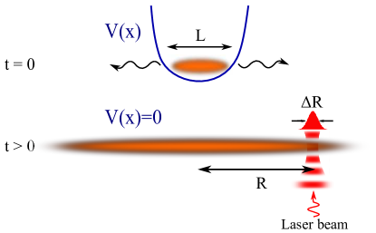
Figure 1: Sketch of ToF experiment with quasi-one-dimensional Bose gas. At $t=0$ the atoms, initially confined to a tube of length $L$, are released form the trap. Interactions between the particles are typically short ranged, and become quickly negligible due to the rapid expansion in transverse direction (not shown here). After propagation time $t$, the density profile of the expanded cloud is investigated by taking an absorption image at position $R$ with a laser beam of waist $\Delta R$. Atoms expand freely after release from the trap, and the distribution of the measured intensity provides direct information on the structure of the initial quantum state.

To demonstrate this approach, we analyze the fingerprints of abundant quantum fluctuations on one dimensional interacting quasi-condensates, and determine the complete distribution of the time of flight image. The particular setup considered is sketched in Fig. 1: a one dimensional Bose gas, confined to a tube of length $L$, is suddenly released from the trap. Due to the rapid expansion in the tightly confined directions (not shown in Fig. 1), the interactions become quickly negligible, and it is enough to consider a free, one dimensional propagation along the longitudinal axis focusing1 . After expansion time $t$, the density profile is imaged by a laser beam at position $R$, which measures the integrated density of particles within the spotsize of the laser, $\Delta R$,

$$\hat{I}_{R,\Delta R}(t)\equiv\int_{-\infty}^{\infty}{\rm d}x\,e^{-(x-R)^{2}/(2\Delta R^{2})}\hat{\psi}^{\dagger}(x,t)\hat{\psi}(x,t).$$ (1)

Here $\hat{\psi}(x,t)$ denotes the bosonic field operator, and we assumed laser a Gaussian laser intensity profile footnote1 . Since bosons propagate freely during the ToF expansion, Eq. (1) provides information on the correlations in the initial state of the system at time $t=0$. In particular, for $R\gg L$ and $\Delta R\ll R$, the measured intensity can be interpreted as the number of particles $\hat{N}_{p}$ with a given initial momentum, $p=mR/t$ ToF . Let us note that the same information about momentum correlations can also be obtained by performing another experimental procedure, the focusing technique  focusing0 ; focusing1 ; focusing (see Appendix C). As we discuss later, apart from minor corrections, our results apply for this type of measurement as well footnote4 , which offers, however, a more accurate approach to measuring distributions in momentum space than the usual ToF technique.

We determine the full distribution of the operator $\hat{I}_{R,\Delta R}$, and show that it contains important information on the quantum fluctuations of the condensate, leading to the emergence of several universal distribution functions. Analysing first the image of a $T\approx 0$ temperature condensate, we show that intensity distributions at finite momenta follow Gamma distribution, and reflect squeezing. The signal of zero momentum particles is, on the other hand, shown to follow a Gumbel distribution in the weakly interacting limit, a characteristic universal distribution of extreme value statistics, and reflecting large correlated particle number fluctuations of the quasi-condensate. We also extend our calculations to finite temperatures and show that the predicted Gumbel distribution should be observable at realistic temperatures for typical system parameters. Then we study the image of the condensate after a quench, and show how thermalization of the condensate manifests itself as a crossover to an - also universal - exponential distribution in the time of flight full counting statistics.

II Theoretical framework

To reach our main goal and to determine the full distribution of $\hat{I}_{R,\Delta R}(t)$ for a one dimensional interacting Bose gas, we shall make use of Luttinger-liquid theory, Imambekov1 ; Imambekov2 and compute all moments of $\hat{I}_{R,\Delta R}$ to show that for long times of flight and large enough distances

$$\langle\hat{I}^{n}_{R,\Delta R}\rangle(t)\to\int_{0}^{\infty}{\rm d}I\;I^{n}\,W_{p}(I)\;$$ (2)

with $n$ positive integer. The function $W_{p}(I)$ can be viewed as the probability distribution function (PDF) of the intensity, measuring the number of particles $N_{p}\sim I$ with momentum $p=mR/t$. Notice that the function $W_{p}(I)$ depends implicitly on the time of flight as well as on the momentum resolution $\Delta p$, suppressed for clarity in Eq. (2).

Luttinger-liquid theory describes the low energy properties of quasi-one-dimensional bosons Cazalilla as well as a wide range of one-dimensional systems Giamarchi . Long wavelength excitations of a Luttinger liquid are collective bosonic modes, described in terms of a phase field, $\hat{\phi}(x)$ Giamarchi . For quasi-condensates, the field operator $\hat{\psi}(x)$ is directly related to this phase operator  Giamarchi

$$\hat{\psi}(x)\approx\sqrt{\rho}\;e^{i\hat{\phi}(x)},$$ (3)

with $\rho$ the average density of the quasi-condensate. Fluctuations of the density generate dynamical phase fluctuations, described by a simple Gaussian action Giamarchi ; ZwergerReview ,

$$S=\dfrac{K}{2\pi}\int{\rm d}t\int{\rm d}x\left(\dfrac{1}{c}\left(\partial_{t}\phi\right)^{2}-c\left(\nabla\phi\right)^{2}\right),$$ (4)

that involves the sound velocity of bosonic excitations, $c$, and the Luttinger parameter, $K$. The dimensionless parameter $K$ characterizes the strength of the interactions: for hard-core bosons $K\to 1$, corresponding to the so-called Tonks-Girardeau limit Girardeau ; TGexperiment , while for weaker repulsive interactions $K>1$, with $K\rightarrow\infty$ corresponding to the non-interacting limit  Giamarchi . The connection between the parameters $c$ and $K$ and the microscopic parameters is model dependent. For a weak repulsive Dirac-delta interaction, $V(x-x^{\prime})=g\,\delta(x-x^{\prime})$, both are determined by perturbative expressions Cazalilla

$$c\cong\sqrt{\dfrac{g\rho}{m}},\quad K\cong\dfrac{\hbar\pi\rho}{mc}=\hbar\pi\sqrt{\dfrac{\rho}{mg}},$$ (5)

with $\hbar$ the Planck constant.

To evaluate the moments of the operator $\hat{I}_{R,\Delta R}(t)$, we first observe that the interactions between the atoms become quickly negligible once the confining potential is turned off and the atoms start to expand. Therefore the fields $\hat{\psi}(x,t)$ evolve almost freely in time for times $t>0$, with a time evolution described by the Feynman propagator, $G(x,t)\sim e^{imx^{2}/(2\hbar t)}/\sqrt{i\,t}$,

$$\hat{\psi}(x,t)=\int{\rm d}x^{\prime}\,G(x-x^{\prime},t)\hat{\psi}(x^{\prime})\,.$$ (6)

For large times, and points far away from the initial position of the condensate one finds that $\hat{\psi}(x,t)$ is approximately equal to the Fourier transform of the field $\hat{\psi}_{p}$ at a momentum $p=mx/t$. This relation becomes exact if, instead of a simple time of flight experiment, one uses the previously mentioned focusing technique (see Appendix C), allowing to reach much better resolutions  focusing0 ; focusing1 ; focusing .

Applying the representation Eq. (3) and the Gaussian action Eq. (4), we can evaluate $\langle\hat{I}_{R,\Delta R}^{n}(t)\rangle$ in any moment Imambekov1 ; Imambekov2 , and construct the intensity distribution $W_{p}(I)$. Using open boundary conditions for the phase operator we obtain, e.g.

$$W_{p}(I)=\int\int_{-\infty}^{\infty}\prod_{j}\dfrac{{\rm d}\tau_{j}\,e^{-\tau_{j}^{2}/2}}{\sqrt{2\pi}}\delta\left(I-\dfrac{N\Delta\widetilde{p}}{\sqrt{2\pi}}g\left(\{\tau_{j}\}\right)\right),$$ (7)

with ${j}=1,2,\dots$ labeling the auxiliary variables $\tau_{j}$ and the function $g\left(\{\tau_{j}\}\right)$ determined by the double integral

$$g\left(\{\tau_{j}\}\right)=\int\int_{-1/2}^{1/2}{\rm d}u\,{\rm d}v\,e^{-\Delta\widetilde{p}^{2}(u-v)^{2}/2+i\,\widetilde{p}(u-v)\left(1-\frac{u+v}{2R/L}\right)}\cdot$$

$$\qquad\exp\left(i\sum_{j}\tau_{j}\;\frac{e^{-\xi_{h}\pi{j}/(2L)}}{\sqrt{K\,{j}}}\left\{\cos\left(\pi\,{j}\,u+\frac{{j}\,\pi}{2}\right)\right.\right.$$

$$\qquad\qquad\qquad\quad-\left.\left.\cos\left(\pi\,{j}\,v+\frac{{j}\,\pi}{2}\right)\right\}\right).$$ (8)

The derivation of Eqs. (7) and (II) is detailed in Appendix A. The healing length $\xi_{h}\equiv\hbar/(mc)$ here serves as a short distance cutoff footnote2 , $N=L\rho$ denotes the total number of particles, and we introduced the dimensionless time of flight momentum and its resolution

$$\widetilde{p}\equiv\dfrac{mR}{t}\dfrac{L}{\hbar}\;\;\;,\quad\Delta\widetilde{p}\equiv\dfrac{m\Delta R}{t}\dfrac{L}{\hbar}\;,$$ (9)

both measured in units of $\hbar/L$.

We note that the intensity measured in a focusing experiment also follows a distribution of the form of Eq. (7), apart from a small change in the function $g\left(\{\tau_{j}\}\right)$. As discussed in Appendix C, in a focusing experiment Eq. (6) yields just the Fourier transform of the field $\hat{\psi}$, and the real space coordinates $R$ and $\Delta R$ are directly proportional to the dimensionless momenta, $\tilde{p}$ and $\Delta\tilde{p}$. As a technical consequence, the term $\exp(-i\tilde{p}(u^{2}-v^{2})L/(2R))$ is absent from the integral giving $g\left(\{\tau_{j}\}\right)$, but for a given $\tilde{p}$ and $\Delta\tilde{p}$, the shape of distribution is hardly affected by this minor modification in the relevant limit, $R\gg L$. Therefore all the results presented below apply also for intensities measured by the refocusing method.

III Equilibrium quantum fluctuations

We evaluated Eqs. (7) and (II) by performing classical Monte Carlo simulations. Already the expectation values, $\langle\hat{I}_{R}\rangle$ carry valuable information, since they account for the size of interaction induced quantum (or thermal) fluctuations of bosons with momentum $p=mR/t$. They are proportional to $\langle\hat{N}_{p}\rangle$ and to the corresponding momentum dependent effective temperatures. The momentum and temperature dependence of $\langle\hat{N}_{p}\rangle$ has been studied theoretically Giamarchi and experimentally TGmomentum ; 1/k4 in detail (see also the following subsections and Appendix D). In an infinitely long Luttinger liquid, in particular, $\langle\hat{N}_{p}\rangle$ falls of as $\sim 1/|p|^{1-1/2K}$ at $T=0$ temperature, while at finite temperatures its value depends on $p$: For small momenta it saturates to a constant proportional to $1/T^{1-1/2K}\approx 1/T$, while at large momenta the power law behavior is recovered. For weak interactions, the cross-over between these two regimes occurs through a regime, where a power law behavior is observed with a modified exponent (see Appendix D).

The average being well understood, here we concentrate on the shape of the full intensity distribution. Therefore, we introduce the normalized intensity

$$\widetilde{I}=\hat{I}_{R,\Delta R}/\langle\hat{I}_{R,\Delta R}\rangle,$$

and determine the corresponding distribution function $\widetilde{W}_{p}(\widetilde{I})$. The intensity distributions for $p=0$ and for typical $p\neq 0$ exhibit drastically different characters; the zero momentum intensity is just associated with particles in the quasi-condensate, while intensities corresponding to $p\neq 0$ reflect quantum fluctuations to states of momentum $p$. We shall therefore discuss these separately.

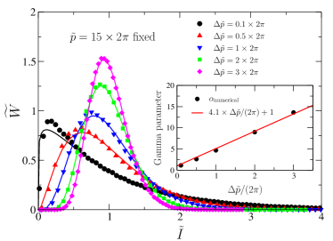
Figure 2: Distribution of normalized intensity $\widetilde{I}$ (symbols) at $T=0$ temperature, plotted for different momentum resolutions, $\Delta\widetilde{p}$. We used $K=10$, $\widetilde{p}=15\times 2\pi$ and $\xi_{h}/L=0.002$. Solid lines are fits with the Gamma distribution from Eq. (10). The distribution smoothly evolves from exponential to Gamma as $\Delta p$ increases, and reflects the two-mode squeezed structure of the Bogoliubov ground state in momenta $p$ and $-p$. Inset: parameter of the fitted Gamma distribution $\alpha$ as a function of $\Delta\widetilde{p}$.

III.1 Zero-temperature intensity distribution of finite momentum particles

Let us first discuss the intensity distribution of finite momentum particles, $p\neq 0$, at $T=0$ temperature, allowing us to take a glimpse at the structure of interaction-generated quantum fluctuations. Fig. 2 shows the typical structure of the distribution function $\widetilde{W}_{p}(\widetilde{I})$ for a moderate Luttinger parameter $K=10$ for various momentum resolutions $\Delta\widetilde{p}$. The shape of $\widetilde{W}_{p}(\widetilde{I})$ has a strong dependence on the resolution $\Delta\widetilde{p}$, and is well described by a Gamma distribution

$$\widetilde{W}_{p\neq 0}(\widetilde{I})\approx\dfrac{\alpha^{\alpha}}{\Gamma(\alpha)}\,\widetilde{I}^{\alpha-1}\,e^{-\alpha\,\widetilde{I}}.$$ (10)

The parameter $\alpha$ here incorporates the momentum resolution, $\Delta\widetilde{p}$, and increases linearly with it (see inset of Fig 2). For good resolutions $\alpha\approx 1$, an exponential distribution is recovered,

$$\widetilde{W}_{p\neq 0}(\widetilde{I})\approx e^{-\widetilde{I}},\phantom{nnn}\text{for }\phantom{nn}{\Delta\widetilde{p}\ll 2\pi}.$$

These observations can be understood in terms of the Bogoliubov approximation Bogoliubov , valid for weak interactions and short system sizes. For small sizes of the laser spot, i. e. $\Delta\widetilde{p}\ll 2\pi$, the intensity, Eq. (1) can be interpreted as the number of particles with dimensionless wave number $p=mR/t$. The Bogoliubov ground state has a two-mode squeezed structure, i.e., particles with momenta $p$ and $-p$ are always created in pairs, implying perfect correlations at the operator level, $\hat{N}_{p}=\hat{N}_{-p}$. This two-mode squeezed structure gives rise to a geometric distribution for the particle number $\hat{N}_{p}$ 2modesqueez , and the exponential intensity distribution observed is just the continuous version of this geometric distribution.

Moreover, Bogoliubov theory predicts vanishing correlation between nonzero momenta $|p|\neq|p^{\prime}|$ Bogoliubov . Therefore, the total number of particles in a given momentum window $\Delta p$ can be viewed as the sum of $\sim\Delta\widetilde{p}/2\pi$ independent, exponentially distributed random variables, with approximately equal expectation values Bogoliubovmomentum

$$\langle\hat{N}_{p}\rangle\approx\frac{\rho\,\hbar\,\pi}{2K|p|}\,.$$ (11)

The Gamma distribution with a parameter $\alpha\propto\Delta\widetilde{p}$ thus arises as the weighted sum of independent exponential variables. The precise prefactor here depends on the shape of the intensity profile in Eq. (1). For a Gaussian profile we find $\alpha\approx 4.1\;\Delta\widetilde{p}/(2\pi)$, while other profiles amount in other numerical prefactors of ${\cal O}(1)$. Though the Bogoliubov approach has only a limited range of validity, a similar crossover from exponential to Gamma distribution persists even for strong interactions (see Appendix F).

III.2 Quasicondensate distribution at $T=0$ temperature

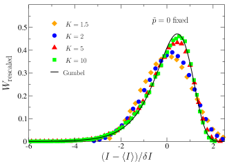
Figure 3: PDF of the normalized variable $(\hat{I}-\langle\hat{I}\rangle)/\delta I$ for $p=mR/t=0$, plotted for different Luttinger parameters $K$, with $\delta I$ referring to standard deviation. We used periodic boundary conditions to compare to analytical results. For weak interactions ($K\gg 1$) the PDF converges to Gumbel distribution, Eq. (12) (solid line), also predicted by a particle number preserving Bogoliubov approach. We used $\Delta\widetilde{p}=0.1\times 2\pi$ and $\xi_{h}/L=0.002$.

Let us now turn to the zero-momentum distribution, corresponding to the number of particles in the quasi-condensate, and exhibiting a completely different behavior, shown in Fig. 3. The distribution, plotted for different interaction strengths $K$, converges quickly to a so-called Gumbel distribution as $K$ increases. This distribution, arising frequently in extreme value statistics Gumbel , is expressed as

$$W_{\rm Gumbel}(\widetilde{I})=\dfrac{\pi}{\sqrt{6}}\;{\rm exp}\left(\dfrac{\pi}{\sqrt{6}}\,\widetilde{I}-\gamma-{\rm exp}\left\{\dfrac{\pi}{\sqrt{6}}\,\widetilde{I}-\gamma\right\}\right),$$ (12)

with $\gamma\approx 0.5772$ the Euler constant.

We can prove that the extreme value distribution (12) follows from particle number conservation combined with the fact that $\hat{N}_{p\neq 0}$ display exponential distributions with expectation values $\langle\hat{N}_{p\neq 0}\rangle\sim 1/|p|$. Particle number conservation relates the fluctuations of the number of particles in the condensate, $\hat{N}_{0}$ with those of $p\neq 0$ particles, $\hat{N}_{0}=N-\sum_{p\neq 0}\hat{N}_{p}$. This can be achieved within the particle number preserving Bogoliubov approach of Ref. Castin by performing a second order expansion in the bosonic fluctuations. As discussed above, all finite momentum particle numbers $\hat{N}_{p\neq 0}$ exhibit exponential distributions with expectation values $\sim 1/|p|$. Therefore, as we show in Appendix E, the distribution of the sum $\sum_{p\neq 0}\hat{N}_{p}$ can be rewritten analytically, and reexpressed as the maximum of a large number of independent, identically distributed exponential random variables, leading to the observed Gumbel distribution.

For strong interactions $K\sim 1$, the zero-momentum distribution starts to deviate form the Gumbel distribution, Eq. (12), considerably. However, the observed distribution is still universal in the sense that it does not depend on the momentum cutoff, and remains unchanged if we consider a Bogoliubov spectrum instead of the linear dispersion relation of a Luttinger liquid.

III.3 Joint probability distribution

Similar to the full distribution function, $W_{p}(I)$, we can generalize usual multipoint correlation functions and define the joint distribution $W_{p_{1},p_{2},\dots}(I_{1},I_{2},\dots)$, corresponding to measuring the intensities $\bigl{\{}\hat{I}_{R_{1}},\hat{I}_{R_{2}},\dots\bigr{\}}$ at positions $R_{i}=p_{i}t/m$. More formally, in analogy with Eq. (2), the joint distribution function $W(I_{R_{1}},I_{R_{2}})$ can be defined through the moments of the variables $\hat{I}_{R_{1}}$ and $\hat{I}_{R_{2}}$,

$$\langle\hat{I}^{n_{1}}_{R_{1}}\hat{I}^{n_{2}}_{R_{2}}\rangle(t)\to\int_{0}^{\infty}{\rm d}I\;I_{1}^{n_{1}}I_{2}^{n_{2}}\,W(I_{1},I_{2}),$$ (13)

for any positive integers $n_{1}$ and $n_{2}$. The previous calculations can be extended to compute these probability distributions with little effort (see Apendix B for details). Without analysing them in detail, here we just briefly discuss the joint distribution function of the of $p=0$ and $p\neq 0$ modes, providing further evidence for the role of particle number conservation behind the emergent extreme value statistics.

The distribution of the normalized variables $\widetilde{I}_{0}$ and $\widetilde{I}_{1}$, corresponding to dimensionless momenta $\widetilde{p}_{0}=0$ and $\widetilde{p}_{1}=2\pi$ is plotted in Fig. 4 for strong ($K=2$) and weak ($K=10$) interactions. The wave number resolution was chosen to be such that particles contributing to the signals ${I}_{0}$ and ${I}_{1}$ have well defined momenta. The joint PDFs reveal strong anticorrelation between the intensities $I_{0}$ and $I_{1}$, interpreted as particle numbers $N_{0}$ and $N_{1}$, for all interaction strengths, persisting for higher values of $p_{1}$. Anticorrelations manifest in the fact that the joint PDF is sharply peaked around the line $\widetilde{I}_{0}+\widetilde{I}_{1}={\rm const.}$, implying that a high intensity $\widetilde{I}_{0}$ is typically accompanied by a low signal $\widetilde{I}_{1}$. The origin of these anticorrelations is particle number conservation: a particle with non-zero wave number $p_{1}$, removed from the quasi-condensate, leaves a ’hole’ behind, eventually appearing as anticorrelation in the joint PDF of $I_{1}$ and $I_{0}$.

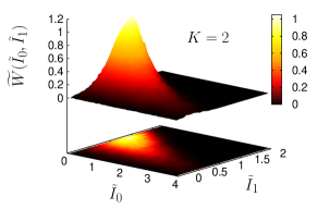
Figure 4: Joint PDF of signals $\widetilde{I}_{0}$ and $\widetilde{I}_{1}$, evaluated for dimensionless momenta $\widetilde{p}_{0}=0$ and $\widetilde{p}_{1}=2\pi$, for strong ($K=2$) and weak ($K=10$) interactions at $T=0$ temperature. The anticorrelation, observable for any interaction strength, reflects particle number conservation. Particles with non-zero wave numbers $p_{1}$, leave holes behind in the quasi-condensate.

III.4 Finite temperature effects and thermal depletion of the quasi-condensate

So far we focused on the limit of $T=0$ temperature. At finite temperatures, modes with energies $E=p\,c\lesssim k_{B}T$ get thermally excited and, at some point, destroy the quasi-condensate. As we show now, this thermal depletion of the quasi-condensate is controlled by the dimensionless temperature

$$\widetilde{T}=\dfrac{1}{K}\dfrac{k_{B}T}{\Delta},$$ (14)

with $\Delta=h\,c/L$ the ’level spacing’, i.e. the typical separation of sound modes in a condensate of size $L$.

Fig. 5 displays the intensity distribution of the zero-mode, derived in Appendix A, as a function of $\widetilde{T}$ for experimentally relevant parameters experiment ; footnote5 . The PDF retains the characteristic shape of a Gumbel distribution for realistic but small temperatures, $\widetilde{T}\lesssim 1$, though the distribution broadens with increasing temperature. At temperatures $\widetilde{T}\gtrsim 1$, however, the PDF turns quickly into an exponential distribution.

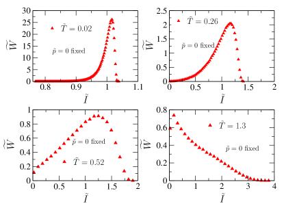
Figure 5: Finite temperature distribution of the normalized zero momentum intensity $\widetilde{I}_{p=0}$, for different dimensionless temperatures $\widetilde{T}=k_{B}T/(K\Delta)$. The PDF crosses over from the zero temperature Gumbel distribution, Eq. (12), to an exponential distribution, as a signature of the thermal depletion of the quasi-condensate by the thermally populated $p\neq 0$ modes. The experimentally accessible temperature range, $T\sim 30\,{\rm nK}\,-\,120\,{\rm nK}$ experiment , corresponds to $\widetilde{T}\sim\,0.12\,-\,0.46$. We used $N=3500$, and $L=39\,\mu{\rm m}$ (density $\rho=90\,\mu{\rm m}^{-1}$), and a chemical potential $\mu/h=1.6\,{\rm kHz}$, implying $K\approx 77$, $c\approx 2,7\,{\rm mm/s}$ and $\xi_{h}/L\approx 0.007$ for ${}^{87}{\rm Rb}$ atoms. We assumed $\Delta\widetilde{p}/(2\pi)=0.1$, corresponding to a time of flight $t=1\,$s, and a real space resolution $\Delta R=12\,\mu{\rm m}$, but shorter times of flight can also be applied using a focusing method, yielding similar images.

This behavior and the crossover scale in Eq. (14) are deeply related to the structure of correlations in a finite temperature Luttinger liquid. At $T=0$ temperature, a bosonic Luttinger liquid exhibits power law correlations at distances larger than the healing length Cazalilla ; Imambekov2 . At finite temperatures, however, these power law correlations turn into an exponential decay beyond the thermal wavelength Cazalilla , where

$$\langle\hat{\psi}^{\dagger}(x)\hat{\psi}(0)\rangle\approx\rho\,\left(\frac{2\xi_{h}}{\lambda_{T}}\right)^{1/2K}e^{-|x|/\xi_{T}},\phantom{nn}\text{for }\,|x|>\lambda_{T}\,.$$ (15)

Notice that the thermal correlation length $\xi_{T}$ appearing here (often denoted by $\lambda_{T}$ in the literature) is proportional to but not identical with the thermal wavelength of the sound modes, denoted here by $\lambda_{T}=\hbar c/(\pi k_{B}T)$; being influenced by the stiffness of the condensate, $\xi_{T}$ is larger by a factor of $2K$ densityripples ,

$$\xi_{T}=2\,K\,\lambda_{T}\,,$$

implying that $\xi_{T}$ can be several orders of magnitude larger than $\lambda_{T}$ in a weakly interacting condensate. Notice that the product $Kc\sim\rho/m$ is independent of the interaction strength by Galilean invariance Kc_Galilei . Thus the correlation length $\xi_{T}\sim\hbar^{2}\rho/(mk_{B}T)$ is independent of the strength of interaction. It is precisely this length scale that appears in Eq (14), which can be re-expressed as $\tilde{T}=L/(\xi_{T}\pi^{2})$. The condition $\tilde{T}\lesssim 1$ thus corresponds to the inequality

$$L\lesssim\xi_{T}\;\pi^{2}$$

ensuring that the phase of the condensate remains close to uniform for sizeable segments of gas. As shown in Appendix D, the number of particles in the $p=0$ mode is also determined by this ratio, $\langle\hat{N}_{0}\rangle\approx N\,2\xi_{T}/L$. Thus $\tilde{T}\lesssim 1$ also implies that at least about 20 % of the particles remain in the homogeneous condensate. As stated earlier in this section, this condition is independent of the interaction strength. Indeed, although the discussion above focused on the weakly interacting limit, $K\gg 1$, we observe a similar crossover to an exponential function even for strong interactions, for which $\lambda_{T}\sim\xi_{T}$ (see Appendix F).

The exponential distribution emerging for $\widetilde{T}\gtrsim 1$ can be understood as a consequence of the thermal depletion of the condensate by low energy $p\neq 0$ modes. Considering the latter naively as particle reservoirs leads to

$${\rm Prob}(\hat{N}_{p=0}=n)\propto e^{-\beta\mu_{\rm eff}n},$$

with some effective chemical potential $\mu_{\rm eff}$, set by the population of low energy modes.

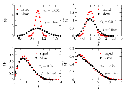
Figure 6: Distribution of the normalized zero momentum intensity $\widetilde{I}_{p=0}$ after an interaction quench, for different holding times, $\tau_{h}=1.3\mu\rm{s}-177\mu\rm{s}$, measured in dimensionless units, $\tilde{\tau}_{h}=\tau_{h}c_{f}/L$. Distributions are plotted for two different quenches of durations $\tau=0.71\mu{\rm s}$ (rapid), and $\tau=71\mu{\rm s}$ (slow). We have used $N=3684$, $L=39\mu\rm{m}$ and a chemical potential $\mu/h=1.6\,{\rm kHz}$, corresponding to $K_{0}=80$, $c_{0}=2.7\rm{mm/s}$, and $\xi_{h}^{0}=0.27\mu\rm{m}$, and assumed an interaction quench to $K_{f}=7$, yielding $c_{f}=c_{0}K_{0}/K_{f}=30.8\;\rm{mm/s}$. We assumed a modest momentum resolution, $\Delta\tilde{p}/(2\pi)=0.1$. Similar to the finite temperature thermalization plotted in Fig. 5, the PDF after a rapid quench crosses over from the equilibrium Gumbel distribution, Eq. (12), to an exponential distribution as $\tilde{\tau}_{h}$ increases, even though the number of excitations in the system remains constant after the quench. For a slower quench, the PDF for short holding times $\tau_{h}$ is much wider than the Gumbel distribution, showing that increasing interactions have time to deplete the quasi-condensate during the quench protocol, resulting in larger particle number fluctuations. As in the case of rapid quench, for larger holding times this PDF crosses over to a thermal distribution.

IV Distribution after interaction quenches

So far we have focused on applying Time of Flight Full Counting Statistics to study equilibrium correlations. Even more interestingly, we can use it to study non-equilibrium dynamics and to gain information about the non-equilibrium states and time evolution of a system after a quantum quench polkovnikovrmp ; dziarmagareview .

Here we demonstrate this perspective by focusing on interaction quenches, i.e., on changing $g$ using a Feshbach resonance  ZwergerReview . For the sake of simplicity, we consider linear quench procedures of $g$, where the product $c(t)K(t)=\hbar\pi\rho/m$ remains constant by Galilean invariance Kc_Galilei , while $c/K$ changes approximately linearly over a quench time $\tau$ footnote3 . After the quench, the atoms are held in the trap for an additional holding time $\tau_{h}$, while the final parameters $c_{f}$ and $K_{f}$ remain constant, and the ToF experiment is performed only afterwards.

For short enough quench times $\tau$, the quench creates abundant excitations. Here we focus on these excitations and concentrate therefore on zero temperature quenches. The initial state is then simply the Gaussian ground state wave function corresponding to the initial parameters $c_{0}$ and $K_{0}$. Moreover, the wave function remains Gaussian during the time evolution quenchGritsev , and can be expressed as

$$\Psi\left(\{\phi_{k}\},t\right)\sim\prod_{k>0}\exp\left(-\sigma_{k}(t)\,\phi_{k}\phi_{-k}\right),$$

with the parameters $\sigma_{k}(t)$ obeying simple differential equations  quenchGritsev . This observation allows us to evaluate the full distribution of the intensity $\tilde{I}_{p}$, by only slightly modifying the derivation outlined in Appendix A.

Fig. 6 shows the intensity distribution of the zero mode, $\tilde{I}_{0}$, for a large quench between Luttinger parameters $K_{0}=80$ and $K_{f}=7$, as a function of the holding time after the quench, $\tau_{h}$. The distributions are plotted for two different quench times $\tau$.

After a rapid quench, for short holding times the probability density function still resembles the Gumbel distribution, Eq.(12), valid for the equilibrium case. However, we observe a crossover to an exponential distribution upon increasing the holding time, $\tau_{h}$. The phenomenon observed is similar to the finite temperature thermalization plotted in Fig. 5, even though the number of excitations in each mode $k$ is a conserved quantity for the Luttinger model considered here, and the final state is definitely not thermal.

The structure of this non-thermal final state can be understood as follows. After long enough holding times, $\tau_{h}$, the distribution of the particle number $\hat{N}_{p}$ looks thermal for each momentum $p$. Based on this thermal, exponential distribution of $\hat{N}_{p}$, one can define an effective inverse temperature $\beta_{p}$ workstatistics ,

$${\rm Prob}(\hat{N}_{p}=n)\propto e^{-\beta_{p}\varepsilon_{p}n},$$

with $\varepsilon_{p}$ denoting the quasiparticles’ dispersion relation. The non-thermal nature of the state is reflected by the fact that in contrast to a thermal state characterized by a single inverse temperature, $\beta_{p}$ strongly depend on the momentum $p$ workstatistics . Similar pre-thermalization phenomena are encountered in some quench experiments on closed, cold atomic systems, where the long-time expectation value of local observables can be well described by a thermal ensemble, despite the non-equilibrium state of the system greiner2 ; thermalization2 .

For a slower quench, the distribution for short holding times $\tau_{h}$ gets much wider compared to the distribution after a sudden quench. This widening can be understood by noting that the interactions increase during the quench protocol. For slower quenches these stronger interactions have time to deplete the quasi condensate while the quench is performed, manifesting in more pronounced particle number fluctuations for short holding times. For larger holding times, however, we observe a crossover to a thermal distribution, similarly to the case of a rapid quench.

For both quench procedures, the time scale of thermalization of the zero-mode is very fast, and for realistic parameters it falls to the range of $\sim 0.1\;\rm{ms}$.

V Conclusions

In this work we have proposed a novel approach to analyse time of flight images, namely to measure the full probability distribution function (PDF) of the intensities in a series of images. Similar to full counting statistics levitov ; nazarov , the PDF of the intensity contains information on the complete distribution of the number of particles $N_{p}$ with a given momentum $p$, beyond its expectation value and variance, and reveals the structure of the quantum state observed and its quantum fluctuations. This so far unexploited information in ToF images reflects the emergent universal behavior of strongly correlated low dimensional quantum systems.

We have demonstrated the perspectives of this versatile method on the specific example of an interacting one-dimensional condensate. We have first focused on the equilibrium signal, and have shown that the intensity distribution of the image for $p\neq 0$ has an exponential character (deformed into a Gamma distribution with decreasing resolution), reflecting the squeezed structure of the superfluid ground state. The $p=0$ intensity distribution, on the other hand, reveals fluctuations of the quasi-condensate, and turns out to be a Gumbel distribution in the weakly interacting limit, a familiar universal distribution from extreme value statistics. We have shown that the Gumbel distribution derives from particle number conservation, combined with large, interaction induced quantum fluctuations of the small momentum modes.

We have also shown that these intriguing fingerprints of quantum fluctuations remain observable in a finite system at small but finite temperatures within the experimentally accessible range, but the predicted Gumbel distribution is destroyed once the small momentum thermal modes thermalize the $p=0$ quasi-condensate mode.

ToF full counting statistics can be used in a versatile way to study non-equilibrium dynamics and thermalization. As an example, we considered an interaction quench, and have shown that the intensity statistics of the $p=0$ mode displays clear signatures of (pre-)thermalization as a function of the holding time after the quench, whereby the original Gumbel distribution, discussed above turns into a quasi-thermal exponential (Gamma) distribution. This universal exponential distribution describes a condensate connected to a particle reservoir, formed by the $p>0$ modes.

One can also go beyond measuring the PDF of the intensity at a given point of the ToF image by measuring the complete joint distribution functions, $W(I_{p},I_{p^{\prime}})$, rather than measuring just intensity correlations, $\langle I_{p}I_{p^{\prime}}\rangle$. As an example, we have determined this joint distribution for the $p=0$ quasi-condensate intensity and the $p\neq 0$ intensities, and have shown that $W(I_{0},I_{p^{\prime}})$ exhibits strong negative correlations, induced by particle number conservation. Clearly, our analysis can be generalized to multipoint distributions, $W(\{I_{p}\})$, still expected to reflect universality, though the experimental and theoretical accessibility becomes less obvious for these complex quantities.

As demonstrated here through the simplest example, ToF full counting statistics is expected to give insight to the exotic quantum states of various interacting quantum systems. Besides investigating the emergent universal behavior of low dimensional quantum systems, Time of Flight Full Counting Statistics could also be applied to study exotic quantum states in higher dimensional, fermionic or even anyonic systems where it is supposed to reflect the quantum statistics of particles. Another interesting direction would be the analysis of ToF full counting statistics at quantum critical points, such as the quantum critical points of the transverse field Ising model or that of spinor condensates spinorreview , e.g., where quantum fluctuations get stronger and bare particles cease to exist. It is also a completely open question, how ToF distributions reflect the structure of a many-body localized state, but the images of chaotic and integrable models are also expected to exhibit different ToF full counting statistics.

Appendix A Probability density function

Here we derive the probability density function of the intensity, $W_{p}(I)$, both for the zero temperature case and for finite temperatures. First we perform the calculations at $T=0$, then we generalize the results to finite temperatures.

In order to derive the PDF at $T=0$, stated in Eqs. (7) and (II), we have to calculate the momenta $\langle\hat{I}_{R,\Delta R}^{n}\rangle(t)$ for all $n$. First we express the intensity $\hat{I}_{R,\Delta R}(t)$ in terms of the field operators at $t=0$ by substituting the free propagator $G(x,t)=\sqrt{\frac{m}{2\pi it}}\,{\rm exp}(imx^{2}/(2t))$ into Eq. (1), and use the density-phase representation (3) to arrive at

$$\hat{I}_{R,\Delta R}(t)= \rho\dfrac{m\Delta R}{\sqrt{2\pi}\,t}\int_{-L/2}^{L/2}{\rm d}x_{1}\int_{-L/2}^{L/2}{\rm d}x_{2}\,e^{-\frac{m^{2}\,\Delta R^{2}}{2\,t^{2}}(x_{1}-x_{2})^{2}}$$

$$e^{\frac{i\,mR}{t}(x_{1}-x_{2})-\frac{im}{2\,t}(x_{1}^{2}-x_{2}^{2})}e^{-i(\hat{\phi}(x_{1},0)-\hat{\phi}(x_{2},0))}.$$ (16)

The $n$th momentum of $\hat{I}_{R,\Delta R}(t)$ involves the $2n$ point correlator of the phase operator. This can be determined by using the Fourier expansion of $\hat{\phi}$, for open boundary conditions given by

$$\hat{\phi}(x)=\frac{1}{\sqrt{L}}\hat{\phi}_{0}+$$

$$\quad\sum_{k>0}\sqrt{\dfrac{\pi}{KL|k|}}e^{-\xi_{h}|k|/2}\cos(k(x+L/2))\left(\hat{b}_{k}+\hat{b}_{k}^{\dagger}\right),$$ (17)

with $k=\pi j/L$, $j\in\mathbb{Z}^{+}$. Here $\hat{b}_{k}^{\dagger}$ and $\hat{b}_{k}$ are bosonic creation and annihilation operators, with $\hat{b}_{k}$ annihilating the ground state of the system. The inverse of the healing length $\xi_{h}$ serves as a momentum cutoff. All ground state expectation values $\langle\hat{I}_{R,\Delta R}^{n}\rangle(t)$ can be calculated by using the normal ordering identity

$$e^{D_{k}\hat{b}_{k}+D_{k}^{*}\hat{b}_{k}^{\dagger}}=e^{D_{k}^{*}\hat{b}_{k}^{\dagger}}e^{D_{k}\hat{b}_{k}}e^{-|D_{k}|^{2}/2}$$

with $D_{k}=\sqrt{\pi/(KL|k|)}e^{-\xi_{h}|k|/2}\cos(k(x+L/2))$, leading to

$$\langle\hat{I}_{R,\Delta R}^{n}\rangle(t)=\left(\dfrac{L\rho\,\Delta\tilde{p}}{\sqrt{2\pi}}\right)^{n}\int...\int_{-1/2}^{1/2}\prod_{i=1}^{n}({\rm d}u_{i}{\rm d}v_{i}\,C(u_{i},v_{i}))\cdot$$

$$\qquad\exp\left(-\sum_{j>0}\frac{e^{-\xi_{h}\pi j/L}}{2Kj}\left[\sum_{i=1}^{n}\left\{\cos\left(\pi ju_{i}+\frac{j\pi}{2}\right)\right.\right.\right.$$

$$\qquad\qquad\qquad\quad-\left.\left.\left.\cos\left(\pi jv_{i}+\frac{j\pi}{2}\right)\right\}\right]^{2}\right),$$ (18)

with

$$C(u,v)=e^{-\frac{\Delta\tilde{p}^{2}}{2}(u-v)^{2}+i\,\tilde{p}(u-v)\left(1-\frac{u+v}{2R/L}\right)},$$ (19)

and dimensionless variables $\tilde{p}$ and $\Delta\tilde{p}$ given by Eq. (9).

The quadratic sum appearing in the exponent of Eq. (A) can be decoupled by applying the Hubbard-Stratonovich transformation, performed by introducing a new integration variable $\tau_{j}$ for every index $j$,

$$\exp\left(-\frac{e^{-\xi_{h}\pi j/L}}{2Kj}\left[\sum_{i=1}^{n}\left\{\cos\left(\pi ju_{i}+\frac{j\pi}{2}\right)\right.\right.\right.$$

$$\qquad\qquad\qquad\quad-\left.\left.\left.\cos\left(\pi jv_{i}+\frac{j\pi}{2}\right)\right\}\right]^{2}\right)=$$

$$\int_{-\infty}^{\infty}\dfrac{{\rm d}\tau_{j}}{\sqrt{2\pi}}e^{-\tau_{j}^{2}/2}\exp\left(i\,\tau_{j}\frac{e^{-\xi_{h}\pi j/(2L)}}{\sqrt{Kj}}\times\right.$$

$$\qquad\left.\sum_{i=1}^{n}\left\{\cos\left(\pi ju_{i}+\frac{j\pi}{2}\right)-\cos\left(\pi jv_{i}+\frac{j\pi}{2}\right)\right\}\right).$$

By substituting this expression into Eq. (A), the integrals over different pairs of variables $\{u_{i},v_{i}\}$ can be performed independently, and we arrive at

$$\langle\hat{I}_{R,\Delta R}^{n}\rangle(t)=\left(\dfrac{L\rho\,\Delta\tilde{p}}{\sqrt{2\pi}}\right)^{n}\int_{-\infty}^{\infty}\prod_{j>0}\dfrac{{\rm d}\tau_{j}}{\sqrt{2\pi}}\,e^{-\tau_{j}^{2}/2}g\left(\{\tau_{j}\}\right)^{n},$$

with $g\left(\{\tau_{j}\}\right)$ given by Eq. (II). Comparing this result with Eq. (2) shows, that the distribution of $\hat{I}_{R,\Delta R}(t)$ can indeed be described by a PDF, given by Eqs. (7) and (II).

Now we generalize these results to $T>0$ temperatures. The Fourier expansion of the phase operator, Eq. (A), together with the thermal occupation of the modes, $\langle\hat{b}_{k}^{\dagger}\hat{b}_{k}\rangle=1/(e^{\beta ck}-1)$, implies

$$\langle e^{i\hat{\phi}(x)-i\hat{\phi}(y)}\rangle=\exp\left(-\sum_{j>0}\frac{e^{-\xi_{h}\pi j/L}}{2K\tanh(\beta c\pi j/(2L))}\times\right.$$

$$\qquad\quad\left.\left[\cos\left(\pi jx+\frac{j\pi}{2}\right)-\cos\left(\pi jy+\frac{j\pi}{2}\right)\right]^{2}\right).$$

The only difference compared to the expectation value at $T=0$ temperature is the appearance of the thermal occupation factor $\tanh(\beta c\pi j/(2L))$. By repeating the derivation above, we find that the distribution function still takes the form Eq. (7), but with a modified function $g_{T}\left(\{\tau_{j}\}\right)$ given by

$$g_{T}\left(\{\tau_{j}\}\right)=\int\int_{-1/2}^{1/2}{\rm d}u\,{\rm d}v\,C(u,v)\times$$

$$\qquad\exp\left(i\sum_{j}\tau_{j}\;\frac{e^{-\xi_{h}\pi{j}/(2L)}}{\sqrt{K\,j\tanh(\frac{\beta c\pi j}{2L})}}\left\{\cos\left(\pi\,{j}\,u+\frac{{j}\,\pi}{2}\right)\right.\right.$$

$$\qquad\qquad\qquad\quad-\left.\left.\cos\left(\pi\,{j}\,v+\frac{{j}\,\pi}{2}\right)\right\}\right).$$

Appendix B Joint distribution function

In this appendix we derive a numerically tractable expression for the joint PDF at $T=0$ temperature, defined in Eq. (13), by calculating the momenta $\langle\hat{I}_{1}^{n_{1}}\hat{I}_{2}^{n_{2}}\rangle(t)$ for all $n_{1}$ and $n_{2}$. Here we introduced the shorthand notation $\hat{I}_{1}\equiv\hat{I}_{R_{1},\Delta R_{1}}$. By using Eq. (A) and the Fourier expansion of the phase operator, Eq. (A), we arrive at

$$\langle\hat{I}_{1}^{n_{1}}\hat{I}_{2}^{n_{2}}\rangle(t)=\left(\dfrac{L\rho}{\sqrt{2\pi}}\right)^{n_{1}+n_{2}}\Delta\tilde{p}_{1}^{n_{1}}\Delta\tilde{p}_{2}^{n_{2}}$$

$$\int...\int_{-1/2}^{1/2}\prod_{i=1}^{n_{1}}({\rm d}u_{i}{\rm d}v_{i}\,C_{1}(u_{i},v_{i}))\prod_{l=1}^{n_{2}}({\rm d}\tilde{u}_{l}{\rm d}\tilde{v}_{l}\,C_{2}(\tilde{u}_{l},\tilde{v}_{l}))\cdot$$

$$\exp\left(-\sum_{j>0}\frac{e^{-\xi_{h}\pi j/L}}{2Kj}\left[\sum_{i=1}^{n_{1}}\left\{\cos\left(\pi ju_{i}+\frac{j\pi}{2}\right)\right.\right.\right.$$

$$-\left.\left.\left.\cos\left(\pi jv_{i}+\frac{j\pi}{2}\right)\right\}+\sum_{l=1}^{n_{2}}\left\{\cos\left(\pi j\tilde{u}_{l}+\frac{j\pi}{2}\right)\right.\right.\right.$$

$$\qquad\qquad\left.\left.\left.-\cos\left(\pi j\tilde{v}_{l}+\frac{j\pi}{2}\right)\right\}\right]^{2}\right),$$ (20)

with $C_{i}(u,v)$ given by Eq. (19) with parameters $R_{i}$ and $\Delta R_{i}$ for $i=1,2$.

Similarly to the calculation presented in Appendix A, the quadratic sum appearing in the exponent of Eq. (B) can be decoupled by applying a Hubbard-Stratonovich transformation. By introducing a new integration variable $\tau_{j}$ for every index $j$, and performing the integrals over different pairs of variables $\{u_{i},v_{i}\}$ and $\{\tilde{u}_{l},\tilde{v}_{l}\}$ independently, we arrive at

$$\langle\hat{I}_{1}^{n_{1}}\hat{I}_{2}^{n_{2}}\rangle(t) =\left(\dfrac{L\rho}{\sqrt{2\pi}}\right)^{n_{1}+n_{2}}\Delta\tilde{p}_{1}^{n_{1}}\Delta\tilde{p}_{2}^{n_{2}}\texttimes$$

$$\int_{-\infty}^{\infty}\prod_{j>0}\dfrac{{\rm d}\tau_{j}}{\sqrt{2\pi}}\,e^{-\tau_{j}^{2}/2}g_{1}\left(\{\tau_{j}\}\right)^{n_{1}}g_{2}\left(\{\tau_{j}\}\right)^{n_{2}},$$

with $g_{i}\left(\{\tau_{j}\}\right)$ given by Eq. (II) with parameters $R_{i}$ and $\Delta R_{i}$ for $i=1,2$. Comparing this expression to the definition of the joint distribution, Eq. (13), we find that

$$W(I_{1},I_{2})=\int\int_{-\infty}^{\infty}\prod_{j}\dfrac{{\rm d}\tau_{j}\,e^{-\tau_{j}^{2}/2}}{\sqrt{2\pi}}\times$$

$$\delta\left(I_{1}-\dfrac{N\Delta\widetilde{p_{1}}}{\sqrt{2\pi}}g_{1}\left(\{\tau_{j}\}\right)\right)\delta\left(I_{2}-\dfrac{N\Delta\widetilde{p_{2}}}{\sqrt{2\pi}}g_{2}\left(\{\tau_{j}\}\right)\right).$$

The distribution can be evaluated by performing a Monte Carlo simulation for the normal random variables $\tau_{j}$, and calculating the two dimensional histogram for $I_{1}$ and $I_{2}$.

Appendix C Focusing technique

Besides the ToF measurements, the focusing technique provides an alternative way to access the momentum distribution focusing0 ; focusing1 ; focusing . The strong transverse confinement of the quasi one dimensional system is abruptly switched off, while the weak longitudinal confinement is replaced by a strong harmonic trap of frequency $\omega$ footnote3 , and the gas is imaged after a quarter time period, $t=T/4=\pi/(2\omega)$.

To express the intensity (1) in this case with the field operators at time $t=0$, we have to replace the free propagator in Eq. (6) by that of the harmonic oscillator $G_{\rm osc}(x,y,t=T/4)={e^{-i\,x\,y/l_{0}^{2}}}/({l_{0}\sqrt{2\pi\hbar\,i}})$, with $l_{0}=\sqrt{\hbar/(m\omega)}$ the oscillator length of the strong trapping potential. In this case, Eqs. (6) thus simply yields the Fourier transform of the field at $t=0$,

$$\hat{\psi}(R,t=T/4)\sim\hat{\psi}_{p}$$

at a momentum $p=\hbar R/l_{0}^{2}$. Thus the intensity measured at $R$ is directly proportional to the number of particles $\hat{N}_{p}$ in this case. Performing calculations similar to those sketched in Appendix A, we arrive at Eqs.  (7) and Eq. (II), with the weight function  (19) replaced by

$$C(u,v)=\exp\left(-\dfrac{\Delta\tilde{p}_{\rm osc}^{2}}{2}(u-v)^{2}+i\,\tilde{p}_{\rm osc}(u-v)\right).$$

and the dimensionless momentum and momentum resolution expressed as $\tilde{p}_{\rm osc}={R\,L}/{l_{0}^{2}}$ and $\Delta\tilde{p}_{\rm osc}={\Delta R\;L}/{l_{0}^{2}}$. Apart from these minor corrections, all our calculations can be performed for focusing experiments, and while this method allows to use shorter measurement times, the conclusions in the main text remain unaltered.

Appendix D The expectation value of $\hat{I}_{R,\Delta R}(t)$

In this appendix we investigate the expectation value of the intensity $\hat{I}_{R,\Delta R}(t)$, scaled out from the distribution functions calculated in the main text.

In order to investigate the temperature dependence of the expectation value, we plotted $\langle\hat{I}_{R,\Delta R}(t)\rangle/N$ as a function of dimensionless momentum $\tilde{p}/(2\pi)$ for different dimensionless temperatures $\tilde{T}$ in Fig. 7. We concentrated on the weakly interacting regime, keeping the Luttinger-parameter, $K=10$, constant. The low temperature results show pronounced oscillations, originating from the presence of the quasi-condensate due to finite size effects. For higher temperatures, the intensity $\langle\hat{I}_{R,\Delta R}(t)\rangle$ increases for non-zero momenta $\tilde{p}=O(2\pi)$, while the zero-momentum expectation value decreases due to the depletion of the condensate. Moreover, we can distinguish two momentum regions, corresponding to different behavior of the expectation value. For momenta much smaller than the thermal wavelength, $p\ll\hbar/\lambda_{T}$ (or $\tilde{p}/(2\pi)\ll\pi K\tilde{T}$ in dimensionless variables), the expectation value of the intensity is well approximated by the Fourier transform of Eq. (15), yielding

$$\langle\hat{N}_{p}\rangle\approx N\,\left(\frac{2\xi_{h}}{\lambda_{T}}\right)^{1/2K}\dfrac{2\xi_{T}/L}{1+(p\,\xi_{T}/\hbar)^{2}}.$$

This expression predicts a power law decay $\langle\hat{I}_{R,\Delta R}(t)\rangle\sim 1/p^{2}$ for momenta $\hbar/\xi_{T}\ll p\ll\hbar/\lambda_{T}$. However, for even larger momenta, $p\gg\hbar/\lambda_{T}$, the short distance behaviour of the correlation function $\langle\hat{\psi}^{\dagger}(x)\hat{\psi}(0)\rangle$ becomes important, and it is not appropriate to approximate it by the simple exponential function Eq. (15). In this region the expectation value of the intensity converges to the zero temperature result, corresponding to a different power law behavior $\langle\hat{I}_{R,\Delta R}(t)\rangle\sim 1/p^{1-1/2K}\approx 1/p$.

This crossover between different power law decays is only observable in the limit of weak interactions, where $\lambda_{T}\ll\xi_{T}$, thus $\hbar/\xi_{T}\ll p\ll\hbar/\lambda_{T}$ is satisfied in a wide momentum range. In this case the Bogoliubov approximation is also valid, thus the same $\sim 1/p^{2}$ decay can also be explained by applying the Bogoliubov approach.

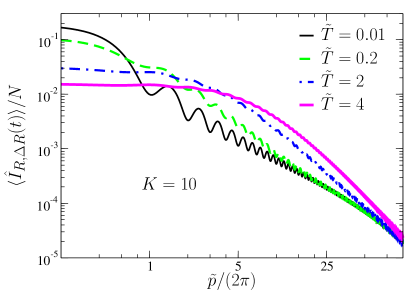
Figure 7: Expectation value $\langle\hat{I}_{R,\Delta R}(t)\rangle/N$ plotted as a function of dimensionless wave number $\tilde{p}/(2\pi)$, for different dimensionless temperatures $\tilde{T}$, with parameters $K=10$, $\xi_{h}/L=0.002$ and $\Delta\tilde{p}=0.1\times 2\pi$, using logarithmic scale on both axis. As $T$ increases, the expectation value develops a wide flat region for small momenta $p\ll\hbar/\xi_{T}$. For larger momenta $\hbar/\xi_{T}\ll p\ll\hbar/\lambda_{T}$, the intensity shows a power law decay $\sim 1/p^{2}$. This behaviour can be explained by the exponential decay of two-point correlations in finite temperature Luttinger-liquids, Eq. (15), with correlation length $\xi_{T}$. For even larger momenta $p\gg\hbar/\lambda_{T}$, we get back the zero temperature results, resulting in a crossover to the different power law behavior $\langle\hat{I}_{R,\Delta R}(t)\rangle\sim 1/p$.

As expected, Bogoliubov theory is also able to account for the cross-over discussed above. According to Eq. (11), the zero temperature Bogoliubov calculation gives $\langle\hat{N}_{p}\rangle\sim 1/|p|$. This result can be generalized to finite temperatures by including the appropriate Bose function, and taking into account the low energy dispersion relation $\varepsilon_{p}=c|p|$, resulting in

$$\langle\hat{N}_{p}\rangle\sim\dfrac{\coth(\beta c|p|/2)}{|p|}\sim 1/p^{2}.$$

Here the last approximation is valid for $p\ll 2k_{B}T/c\approx\hbar/\lambda_{T}$. As already mentioned, this $\sim 1/p^{2}$ decay is consistent with the numerical results plotted in Fig. 7.

Appendix E Gumbel distribution

In this appendix we show that the Gumbel distribution (12), arising for weak interactions, can be derived from the structure of the Bogoliubov ground state, by taking into account particle number conservation. In this perturbative approach, the PDF (12) emerges as the distribution of the normalized operator giving the number of particles with zero momentum,

$$\tilde{N}_{0}=\dfrac{\hat{N}_{p=0}-\langle\hat{N}_{p=0}\rangle}{\delta N_{p=0}}.$$

Here $\langle\hat{N}_{p=0}\rangle$ denotes the expectation value, and $\delta N_{p=0}$ is the standard deviation. For simplicity, we perform the calculations using periodic boundary conditions.

As already noted in the main text, particle number conservation implies

$$\hat{N}_{p=0}=N-\sum_{p\neq 0}\hat{N}_{p},$$ (21)

with $N$ denoting the total number of particles. Moreover, the two mode squeezed structure of the ground state in non-zero momenta $p$ and $-p$, resulting in a perfect correlation $\hat{N}_{p}=\hat{N}_{-p}$, leads to an exponential distribution for the random variable $(\hat{N}_{p}+\hat{N}_{-p})/N$, with expectation value $\hbar\pi/(KL|p|)$ Bogoliubov (see Eq. (11)). For PBC the momentum can only take values $p=2\pi n\hbar/L$, so the PDF of the sum $\sum_{p\neq 0}\hat{N}_{p}/N$ can be written as

$$P\left(\sum_{p\neq 0}\hat{N}_{p}/N=x\right)=\prod_{i=1}^{n_{c}}(2Kn)\int_{0}^{\infty}{\rm d}x_{1}\,e^{-2K\,x_{1}}\times$$

$$\int_{0}^{\infty}{\rm d}x_{2}\,e^{-2K\,2\,x_{2}}...\int_{0}^{\infty}{\rm d}x_{n_{c}}e^{-2K\,n_{c}\,x_{n_{c}}}\delta\left(x-\sum_{i=1}^{n_{c}}x_{i}\right).$$ (22)

Here $n_{c}\sim L/\xi_{h}$ denotes a cutoff in momentum space, restricting the momentum $p$ to the low energy region, described by linear dispersion relation.

The PDF (E) can be rewritten by introducing new integration variables $z_{1}=x_{n_{c}}$, $z_{2}=x_{n_{c}}+x_{n_{c}-1}$, …, and $z_{n_{c}}=\sum_{i=1}^{n_{c}}x_{i}$ as

$$P\left(\sum_{p\neq 0}\hat{N}_{p}/N=x\right)=(2K)^{n_{c}}\,n_{c}!\,\times$$

$$\int_{0}^{\infty}{\rm d}z_{1}\int_{z_{1}}^{\infty}{\rm d}z_{2}...\int_{z_{n_{c}-1}}^{\infty}{\rm d}z_{n_{c}}e^{-2K\sum_{i=1}^{n_{c}}z_{i}}\,\delta\left(x-z_{n_{c}}\right).$$

This result shows, that the PDF associated to the operator $\sum_{p\neq 0}\hat{N}_{p}/N$ is equivalent to the distribution of the maximum of $n_{c}$ independent, exponentially distributed random variables, with equal expectation values $1/(2K)$. This observation follows from noting, that the integrand describes independent exponential random variables, subject to the constraint $z_{1}<z_{2}<...<z_{n_{c}}$, with the factor $n_{c}!$ taking into account all possible orderings of these $n_{c}$ variables. This interpretation explains the emergence of the extreme value distribution $W_{\rm Gumbel}$.

The cumulative distribution function of the maximum of independent random variables can be easily calculated, leading to the probability

$${\rm Prob}\left(\tilde{N}_{0}<x\right)={\rm Prob}\left(\sum_{p\neq 0}\dfrac{\hat{N}_{p}}{N}>\sum_{p\neq 0}\dfrac{\langle\hat{N}_{p}\rangle}{N}-x\dfrac{\delta N_{p=0}}{N}\right)$$

$$=1-\left(1-{\rm exp}\left\{-2K\left(\sum_{p\neq 0}\dfrac{\langle\hat{N}_{p}\rangle}{N}-x\dfrac{\delta N_{p=0}}{N}\right)\right\}\right)^{n_{c}}$$

$$\approx 1-{\rm exp}\left(-n_{c}\,{\rm exp}\left\{-2K\left(\sum_{p\neq 0}\dfrac{\langle\hat{N}_{p}\rangle}{N}-x\dfrac{\delta N_{p=0}}{N}\right)\right\}\right),$$ (23)

with the approximation in the third line valid for large $K$. Here the expectation value $\sum_{p\neq 0}\langle\hat{N}_{p}\rangle/N$ is given by

$$\dfrac{\langle\hat{N}_{p}\rangle}{N}=\sum_{n=1}^{n_{c}}\dfrac{1}{2Kn}.$$

Moreover, using the particle number conservation (21), and the variances the variables $\hat{N}_{p\neq 0}$, the standard deviation $\delta N_{p=0}/N$ can be calculated as

$$\dfrac{\delta N_{p=0}}{N}=\sqrt{\sum_{n=1}^{n_{c}}\left(\dfrac{1}{2Kn}\right)^{2}}\approx\dfrac{\pi}{2\sqrt{6}K},$$

taking the limit of large cutoff $n_{c}$ in the last step. Substituting these results into (E) allows us to take the $n_{c}\rightarrow\infty$ limit, resulting in the cumulative distribution function

$${\rm Prob}\left(\tilde{N}_{0}<x\right)\approx 1-{\rm exp}\left\{-\exp\left(\dfrac{\pi}{\sqrt{6}}x-\gamma\right)\right\},$$

with $\gamma$ denoting the Euler constant, defined by the relation

$$\gamma=\lim_{n_{c}\rightarrow\infty}\,\sum_{n=1}^{n_{c}}\dfrac{1}{n}-{\rm log}\,n_{c}.$$

By taking the derivative of this cumulative distribution function, we arrive at the PDF of the Gumbel distribution, Eq. (12).

Appendix F Numerical results for strong interactions

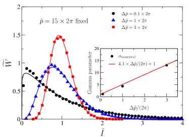
Figure 8: Distribution of normalized intensity $\widetilde{I}$ (symbols) at $T=0$ for stronger interactions, and fits with the Gamma distribution from Eq. (10) (solid lines), plotted for different momentum resolutions $\Delta\widetilde{p}$. We used $K=2$, $\widetilde{p}=15\times 2\pi$ and $\xi_{h}/L=0.002$. Similarly to the limit of weak interactions, the distribution smoothly evolves from exponential to Gamma as $\Delta p$ increases. Inset: parameter of the fitted Gamma distribution $\alpha$ as a function of $\Delta\widetilde{p}$, increasing approximately linearly with the same slope as in the weakly interacting limit.

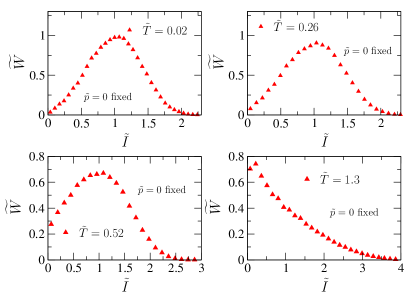
Figure 9: Finite temperature distribution of the normalized zero momentum intensity $\widetilde{I}_{p=0}$ for strong interactions, using different dimensionless temperatures $\widetilde{T}=k_{B}T/(K\Delta)$. The PDF crosses over from the zero temperature limit (deviating from Gumbel distribution due to strong interactions) to an exponential distribution, as a signature of the depletion of the zero mode by the thermally populated $p\neq 0$ modes. As in the limit of weak interactions, the crossover is governed by the dimensionless temperature $\tilde{T}$. We used $K=1.5$, $\Delta\widetilde{p}/(2\pi)=0.1$ and $\xi_{h}/L\approx 0.002$.

In the figures of the main text we concentrated mostly on the limit of weak interactions. Here we present additional numerical results, corresponding to stronger interactions.

By analyzing the equilibrium quantum fluctuations at $T=0$ temperature, we have shown in Sec. III.1 that the distribution of the intensity at finite momentum crosses over from exponential to Gamma distribution with increasing momentum resolution $\Delta p$. We plotted this crossover for weak interactions in Fig. 2. In Fig. 8 we show the same crossover for stronger interactions $K=2$. We find that the parameter of the fitted Gamma distribution, Eq. (10), increases approximately linearly with $\Delta p$, with the same slope as in the limit of weak interactions.

We considered the finite temperature distribution of the zero mode in Sec. III.4. In the limit of weak interactions, plotted in Fig. 5 of the main text, we found a crossover from the zero temperature Gumbel distribution to an exponential distribution, as the temperature is increased and thermal fluctuations deplete the quasi-condensate. We observe a similar crossover for strong interactions $K=1.5$, by plotting the zero-momentum distributions for different dimensionless temperatures $\tilde{T}$ in Fig. 9. For such strong interactions, the distribution at $T=0$ deviates from the Gumbel distribution considerably (see also Fig. 3 in the main text), but a clear crossover from the $T=0$ limit to an exponential distribution, governed by the dimensionless temperature $\tilde{T}$, still persists.

References

- (1) H. E. Stanley, Introduction to Phase Transitions and Critical Phenomena, Oxford University Press (1971).
- (2) J. Cardy, Scaling and Renormalization in Statistical Physics, Cambridge University Press (1996).
- (3) L. P. Kadanoff, Statistical Physics - Statics, Dynamics and Renormalization, World Scientific Publishing Company (2000).
- (4) S. Sachdev, Quantum Phase Transitions, Cambridge University Press (2001).
- (5) T. Giamarchi, Quantum Physics in One Dimension, International Series of Monographs on Physics, 2003).
- (6) A. O. Gogolin, A. A. Nersesyan, and A. M. Tsvelik, Bosonization and strongly correlated systems, Cambridge University Press (1998).
- (7) M. A. Cazalilla, J. Phys. B: AMOP 37, S1-S47 (2004).
- (8) F. D. M. Haldane, Phys. Rev. Lett. 47, 1840 (1981).
- (9) J. van Delft, and H. Schoeller, Bosonization for beginners — refermionization for experts, Ann. Phys. 7, 225 (1998).
- (10) A. Perrin, R. Bücker, S. Manz, T. Betz, C. Koller, T. Plisson, T. Schumm and J. Schmiedmayer, Nat. Phys. 8, 195 (2012).
- (11) I. Safi, and H. J. Schulz, Phys. Rev. B 52, R17040(R) (1995).
- (12) S. Tarucha, T. Honda, and T. Saku, Solid State Commun. 94, 413 (1995).
- (13) A. R. Goñi, A. Pinczuk, J. S. Weiner, J. M. Calleja, B. S. Dennis, L. N. Pfeiffer, and K. W. West, Phys. Rev. Lett. 67, 3298 (1991).
- (14) U. Meirav, M. A. Kastner, and S. J. Wind, Phys. Rev. Lett. 65, 771 (1990).
- (15) D. A. Tennant, R. A. Cowley, S. E. Nagler, and A. M. Tsvelik, Phys. Rev. B 52, 13368 (1995).
- (16) S. Hofferberth, I. Lesanovsky, T. Schumm, A. Imambekov, V. Gritsev, E. Demler, and J. Schmiedmayer, Nat. Phys. 4, 489 (2008).
- (17) M. Gring, M. Kuhnert, T. Langen, T. Kitagawa, B. Rauer, M. Schreitl, I. Mazets, D. A. Smith, E. Demler, and J. Schmiedmayer, Science 337, 1318 (2012).
- (18) T. Berrada, S. van Frank, R. Bücker, T. Schumm, J.-F. Schaff, and J. Schmiedmayer, Nat. Commun. 4, 3077 (2013).
- (19) L. S. Levitov, H. Lee, and G. B. Lesovik, Electron counting statistics and coherent states of electric current, J. Math. Phys. 37, 4845 (1996).
- (20) Y. Nazarov, Quantum Noise in Mesoscopic Physics, Nato Science Series, Kluwer (2003)
- (21) Wei Lu, Zhongqing Ji, Loren Pfeiffer, K. W. West, A. J. Rimberg, Nature 423, 422 (2003).
- (22) S. Gustavsson, R. Leturcq, B. Simovič, R. Schleser, T. Ihn, P. Studerus, K. Ensslin, D. C. Driscoll, and A. C. Gossard, Counting statistics of single electron transport in a quantum dot, Phys. Rev. Lett. 96, 076605 (2006).
- (23) V. F. Maisi, D. Kambly, C. Flindt, and J. P. Pekola, Full counting statistics of andreev tunneling, Phys. Rev. Lett. 112, 036801 (2014).
- (24) A. Silva, Phys. Rev. Lett. 101, 120603 (2008).
- (25) T. B. Batalhão, A. M. Souza, L. Mazzola, R. Auccaise, R. S. Sarthour, I. S. Oliveira, J. Goold, G. De Chiara, M. Paternostro, and R. M. Serra, Phys. Rev. Lett. 113, 140601 (2014).
- (26) K. Magishi, S. Matsumoto, Y. Kitaoka, K. Ishida, K. Asayama, M. Uehara, T. Nagata, and J. Akimitsu, Phys. Rev. B 57, 11533 (1998).
- (27) C. Bourbonnais, and D. Jerome, in ”Advances in Synthetic Metals, Twenty years of Progress in Science and Technology”, edited by P. Bernier, S. Lefrant, and G. Bidan (Elsevier, New York, 1999), pp. 206-301.
- (28) L. Venkataraman, and C. M. Lieber Phys. Rev. Lett. 83, 5334 (1999).
- (29) J. Park, S. W. Jung, M.-C. Jung, H. Yamane, N. Kosugi, and H. W. Yeom, Phys. Rev. Lett. 110, 036801 (2013).
- (30) J. R. Ahn, H. W. Yeom, H. S. Yoon, and I.-W. Lyo, Phys. Rev. Lett. 91, 196403 (2003).
- (31) I. Bloch, J. Dalibard and W. Zwerger, Rev. Mod. Phys. 80, 885 (2008).
- (32) E. Altman, E. Demler and M. D. Lukin, Phys. Rev. A 70, 013603 (2004).
- (33) V. Guarrera, N. Fabbri, L. Fallani, C. Fort, K. M. R. van der Stam and M. Inguscio, Phys. Rev. Lett. 100, 250403 (2008).
- (34) B. Fang, A. Johnson, T. Roscilde, and I. Bouchoule, Phys. Rev. Lett. 116, 050402 (2016).
- (35) D. S. Petrov, G. V. Shlyapnikov and J. T. M. Walraven, Phys. Rev. Lett. 85, 3745 (2000).
- (36) A. Görlitz, J. M. Vogels, A. E. Leanhardt, C. Raman, T. L. Gustavson, J. R. Abo-Shaeer, A. P. Chikkatur, S. Gupta, S. Inouye, T. Rosenband and W. Ketterle, Phys. Rev. Lett. 87, 130402 (2001).
- (37) T. Schumm, S. Hofferberth, L. M. Andersson, S. Wildermuth, S. Groth, I. Bar-Joseph, J. Schmiedmayer and P. Krüger, Nat. Phys. 1, 57 (2005).
- (38) V. Gritsev, E. Altman, E. Demler and A. Polkovnikov, Nat. Phys. 2, 705 (2006).
- (39) T. Kitagawa, S. Pielawa, A. Imambekov, J. Schmiedmayer, V. Gritsev and E. Demler, Phys. Rev. Lett. 104, 255302 (2010).
- (40) T. Kitagawa, A. Imambekov, J. Schmiedmayer and E. Demler, New J. Phys. 13, 073018 (2011).
- (41) R. Grimm, M. Weidemüller and Y. B. Ovchinnikov, Adv. At. Mol. Opt. Phys. 42, 95 (2000).
- (42) In case of simply taking a picture of the condensate, would represent the resolution of the optical system.
- (43) M. Girardeau, J. Math. Phys. 1, 516 (1960).
- (44) T. Kinoshita, T. Wenger and D. S. Weiss, Science 305, 1125 (2004).
- (45) Luttinger-liquid theory, being an effective long wave length description, loses its validity below the length scale Giamarchi .
- (46) B. Paredes, A. Widera, V. Murg, O. Mandel, S. Fölling, I. Cirac, G. V. Shlyapnikov, Th. W. Hänsch and I. Bloch, Nature 429, 277 (2004).
- (47) R. Chang, Q. Bouton, H. Cayla, C. Qu, A. Aspect, C. I. Westbrook and D. Clément, arXiv:1608.04693.
- (48) N. N. Bogoliubov, D. V. Shirkov, Introduction To the Theory of Quantized Fields (John Wiley & Sons, 1980).
- (49) Ch. Mora and Y. Castin, Phys. Rev. A 67, 053615 (2003).
- (50) C. Gerry and P. Knight, Introductory Quantum Optics (Cambridge University Press, 2005).
- (51) E. J. Gumbel, Statistical theory of extreme values and some practical applications (Applied Mathematics Series 33, 1954).
- (52) L. Mathey, A. Vishwanath and E. Altman, Phys. Rev. A. 79, 013609 (2009).
- (53) Y. Castin and R. Dum, Phys. Rev. A 57, 3008 (1998).
- (54) S. Manz, R. Bücker, T. Betz, Ch. Koller, S. Hofferberth, I. E. Mazets, A. Imambekov, E. Demler, A. Perrin, J. Schmiedmayer and T. Schumm, Phys. Rev. A 81, 031610(R) (2010).
- (55) A. Imambekov, I. E. Mazets, D. S. Petrov, V. Gritsev, S. Manz, S. Hofferberth, T. Schumm, E. Demler and J. Schmiedmayer, Phys. Rev. A 80, 033604 (2009).
- (56) A. Polkovnikov, K. Sengupta, A. Silva, and M. Vengalattore, Rev. Mod. Phys. 83, 863 (2011).
- (57) J. Dziarmaga, Adv. Phys. 59, 1063 (2010).
- (58) R. Citro, S. De Palo, E. Orignac, P. Pedri and M.-L. Chiofalo, New J. Phys. 10, 045011 (2008).
- (59) A. Polkovnikov and V. Gritsev, Nat. Phys. 4, 478 (2008).
- (60) I. Shvarchuck, Ch. Buggle, D. S. Petrov, K. Dieckmann, M. Zielonkovski, M. Kemmann, T. G. Tiecke, W. von Klitzing, G. V. Shlyapnikov, and J. T. M. Walraven, Phys. Rev. Lett. 89, 270404 (2002).
- (61) Th. Jacqmin, B. Fang, T. Berrada, T. Roscilde, and I. Bouchoule, Phys. Rev. A 86, 043626 (2012).
- (62) S. Tung, G. Lamporesi, D. Lobser, L. Xia, and E. A. Cornell, Phys. Rev. Lett. 105, 230408 (2010).
- (63) In the perturbative limit, Eq. (5), the ratio is directly proportional to the interaction .
- (64) The measurement of the momentum distribution in a ToF experiment requires long expansion times. The drawback of this method is that the much faster expansion of the transverse directions can result in a loss of signal. This problem can be circumvented by the focusing technique, allowing much shorter expansion times and better signal to noise ratios.
- (65) In real experiments the atoms are confined to an optical trap, before being released to propagate freely during the ToF measurement. In our calculations we neglect the confining potential, and consider a homogeneous density with open or periodic boundary conditions for the phase operator. This approximation is justified, if the measured intensity is determined by the quantum fluctuations at the center of trap, where the density varies slowly, allowing a local density approximation.
- (66) Y. Kawaguchia and M. Ueda, Phys. Rep. 520, 253 (2012).
- (67) C. Schwemmer, G. Tóth, A. Niggebaum, T. Moroder, D. Gross, O. Gühne, and H. Weinfurter, Phys. Rev. Lett. 113, 040503 (2014).
- (68) B. Dóra, Á. Bácsi, and G. Zaránd, Phys. Rev. B 86, 161109(R) (2012).
- (69) A. M. Kaufman, M. E. Tai, A. Lukin, M. Rispoli, R. Schittko, Ph. M. Preiss, and M. Greiner, Science 353, 794 (2016).
- (70) M. Rigol, V. Dunjko, M. Olshanii, Nature 452, 854 (2008).
- (71) S. P. Rath, and W. Zwerger, Phys. Rev. A 82, 053622 (2010).
- (72) E. Altman, E. Demler and M. D. Lukin, Phys. Rev. A 70, 013603 (2004).
- (73) S. Fölling, F. Gerbier, A. Widera, O. Mandel, T. Gericke and I. Bloch, Nature 434, 481 (2005).
- (74) T. Rom, Th. Best, D. van Oosten, U. Schneider, S. Fölling, B. Paredes and I. Bloch, Nature 444, 733 (2006).
- (75) Noise correlations, extracted from time of flight images, have already been used as a versatile tool to study strongly correlated many-body systems, see Refs. noise ; folling ; fermionnoise .