The 5 Gyr evolution of sub-M* galaxies

Abstract

We gathered two complete samples of $M_{AB}(r)<-18$ ($M_{star}>10^{9}M_{\odot}$) galaxies, which are representative of the present-day galaxies and their counterparts at 5 Gyr ago. We analysed their 2D luminosity profiles and carefully decomposed them into bulges, bars and discs. This was done in a very consistent way at the two epochs, by using the same image quality and same (red) filters at rest. We classified them into elliptical, lenticular, spiral, and peculiar galaxies on the basis of a morphological decision tree.

We found that at $z=0$, sub-M* ($10^{9}M_{\odot}<M_{star}<1.5\times 10^{10}M_{\odot}$) galaxies follow a similar Hubble Sequence compared to their massive counterparts, though with a considerable larger number of (1) peculiar galaxies and (2) low surface brightness galaxies. These trends persist in the $z\sim 0.5$ sample, suggesting that sub-M* galaxies have not reached yet a virialised state, conversely to their more massive counterparts. The fraction of peculiar galaxies is always high, consistent with a hierarchical scenario in which minor mergers could have played a more important role for sub-M* galaxies than for more massive galaxies.

Interestingly, we also discovered that more than 10% of the sub-M* galaxies at z=0.5 are low surface brightness galaxies with clumpy and perturbed features that suggest merging. Even more enigmatic is the fact that their disc scale-lengths are comparable to that of M31, while their stellar masses are similar to that of the LMC.

1 Introduction

The deepest HST images revealed a plethora of intrinsically faint galaxies at z $\sim$ 1 (Ryan et al. 2007). Because the $\Lambda$-CDM model predicts that galaxies are assembled over cosmic times through the hierarchical merging of progressively more massive sub-units (e.g., White & Rees 1978), possibly combined with massive accretion of cold gas (e.g., Kereš et al. 2009, although see Nelson et al. 2013), it is then expected that the fraction of dwarf galaxies amongst the whole galaxy population increases as a function of redshift $z$. This should be reflected by a steepening of the faint-end slope of the galaxy LF. However, observational results are quite puzzling. On the one hand, first results based on rest-frame UV data indeed detected such an increase (e.g., Ryan et al. 2007, Reddy & Steidel 2009). But on the other hand, more recent results at rest-frame optical wavelengths revealed that the faint-end slope actually appears to remain constant out to $z\sim 4$ (e.g., Marchesini et al. 2012), hence quite in contrast with expectations from the $\Lambda$-CDM model (Khochfar et al., 2007).

Distant sub-M* galaxies (i.e., galaxies with masses smaller than the knee of the LF) have faint apparent magnitudes ($z_{AB}$ $\sim$ 24 at $z=0.5$) that have limited detailed morphological studies and 3D spectroscopy with current facilities until recently. Deep recent HST surveys and 3D observations have now started to investigate their morphological properties (e.g., van der Wel et al. 2014; Kartaltepe et al. 2015; Whitaker et al. 2015) and kinematic properties (e.g., Kassin et al. 2012; Simons et al. 2015; Contini et al. 2016). Besides spirals and ellipticals, other types of galaxies may increasingly appear in the sub-M* range, as mass decreases from $\sim 10^{10}M_{\odot}$ to $\sim 10^{9}M_{\odot}$. These include low surface brightness galaxies (see Zhong et al. 2012 and references therein), tidal dwarf galaxies (TDGs, see Fig. 2 of Kaviraj et al. 2011), and objects more and more similar to dwarfs (i.e., elliptical: dE, spiral: dSp, and irregular: dIrr, see, e.g., Kormendy et al. 2009). Spirals in this mass range form a sequence in the surface brightness vs. absolute magnitude plane together with Irrs and dSphs (see Kormendy et al. 2009, and references therein), which strongly differs from the sequence formed by Ellipticals and dEs.

The goal of this paper is to investigate the detailed morphology of sub-M* galaxies and investigate possible formation mechanisms in comparison with super-M* galaxies. For this, we followed the careful methodology introduced by Delgado-Serrano et al. (2010) for $M_{stellar}>1.5\times 10^{10}$ $M_{\odot}$ galaxies. We present a complete morphological inventory of these galaxies at two epochs (i.e., 0 and 5 Gyr ago), as described in Sect. 2. Methodology and analysis are detailed in Sect. 3. Sect. 4 investigates more specifically low surface brightness galaxies, while a complete morphological classification is presented in Sect. 5. We discuss in Sect. 6 the accuracy of the results and their main limitations, and conclusions are drawn in Sect. 7. Throughout this paper we adopt cosmological parameters with $H_{0}=70$ km.s^-1.Mpc^-1 and $\Omega_{\Lambda}$=0.7. Magnitudes are given in the $AB$ system.

2 Representative samples of nearby and distant galaxies

2.1 Methodology & sample sizes

The morphological classification was done following the classification tree introduced by Delgado-Serrano et al. (2010). This requires two main steps: (1) the analysis of the light distribution and its decomposition into several components (bulge, disc, and bar when necessary), and (2) the analysis of the galaxy color map. These steps are detailed in Sect 3. The global uncertainty associated to any classification is a combination of Poisson random fluctuations due to the finite size $N$ of the sample and possible systematics due to the intrinsic relative (in)accuracy of the classification process (i.e., the fraction of objects that are not properly classified as a result of approximations in the methodology used during the classification, see Sect. 3). While the random uncertainty varies as $\sqrt{N}/N$, i.e., it decreases with larger samples, the systematics are independent of the sample size. Using the Delgado-Serrano et al. (2010) classification tree, we estimated the latter to be $\sim$ 10% from a comparison between morphology and spatially-resolved kinematics (see Neichel et al. 2008). This implies that the total uncertainty (random and systematics) will remain limited by systematics regardless of the sample size once $N$ reaches $\sim$100 galaxies. Note that automatic classification methods lead to even larger systematics (e.g., Neichel et al. 2008, Pović et al. 2015). The sample sizes were therefore fixed to $N=150$ objects.

2.2 Sample selection

2.2.1 Local galaxy sample

Galaxies were selected from the Sloan Digital Sky Survey Release Seven (SDSS DR7, Abazajian et al. 2009). We used the low-$z$ catalogue of the New York University Value Added Galaxy Catalog (NYU-VAGC,  Blanton et al. 2005), which includes absolute magnitudes, $k$-corrections, and extinctions in the $u$ (3551Å), $g$ (4686Å), $r$ (6165Å), $i$ (7481Å), and $z$ (8931Å) bands. Figure 1 shows the relationship between redshift and absolute magnitude in $r$ band, from which we extracted an unbiased volume-limited sample: given a cut in luminosity ($M_{AB}(r)\leq-18$) a redshift cut ($z\leq 0.033$) is necessary to avoid any Malmquist bias. We also defined a lower redshift cut ($z\geq 0.022$) to ensure that the peculiar motions of the closest galaxies could not affect redshift and distance determinations. At this stage the parent sample contained 12,681 galaxies. A representative subsample of 150 galaxies was then selected at random. One galaxy was found to fall on the CCD edge, which was removed from the final sample. Figure 2 compares the distribution of the $r$-band absolute magnitudes for the final sample of 149 galaxies with the $r$-band luminosity function of local galaxies (Blanton et al., 2003). A Kolmogorov-Smirnov test indicates a probability of 99% that both the sample and the local luminosity function are drawn from the same parent distribution. This sample is thus representative of the $M_{AB}(r)\leq-18$ galaxy population in the local Universe. We checked that other properties such as the $g-r$ color and the Petrosian half-light surface brightness (extracted from the NYU-VAGC catalogue) in the final sample and parent samples also follow the same distributions. Luminosities in $r$ band were converted into stellar masses $M_{stellar}$ using the statistical empirical relation between $M_{stellar}/L_{r}$ and the $u-g$ color from Bell et al. (2003).

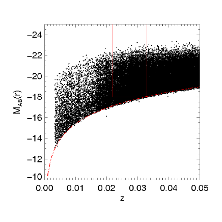
Figure 1: $M_{AB}(r)-z$ plane for the SDSS galaxies. The region delimited by the red solid lines delineates the local volume-limited sample with $M_{AB}(r)\leq-18$ and 0.022$\leq z\leq$0.033.

2.2.2 Distant galaxy sample

The distant sample was selected from the CANDELS/GOODS-South survey (Koekemoer et al. 2011, Grogin et al. 2011). Using SExtractor (Bertin & Arnouts, 1996) in the HST/ACS $B$ (4312Å), $V$ (5915Å), $i$ (7697Å), and $z$ (9103Å) v2.0 images and in the HST/WFC3 $J$ (12486Å) and $H$ (15369Å) v1.0 images, we built our own photometric catalogues, which were then cross-correlated with the catalogue of photometric redshifts from Dahlen et al. (2010). Stellar masses and absolute magnitudes were calculated using the prescription discussed in Bell et al. (2003) (see also Hammer et al. 2005 and references therein). We applied the same luminosity criterion we used in the local sample, i.e., $M_{AB}(r)\leq-18$, and selected sources with photometric redshifts between 0.4 and 0.6, which ensures that the observed light in $z$ band corresponds to a rest-frame emission in $r$ band. The 278 sources thus selected were visual inspected in all bands and contaminating stars were removed from the sample, leading to a final sample of 229 galaxies with $M_{AB}(r)\leq-18$ and $0.4\leq z_{phot}\leq 0.6$. 150 galaxies were then selected from this parent sample at random. The comparison between the $M_{AB}(r)$ distribution of the final sample and the $R$-band luminosity function of galaxies at redshifts 0.4 to 0.6 from Ilbert et al. (2005) is shown in Fig. 2. A Kolmogorov-Smirnov test gives a probability of 99.9% that the sample and the luminosity function are drawn from the same parent distribution, which evidences the representativity of the distant sample.

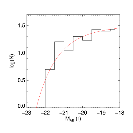
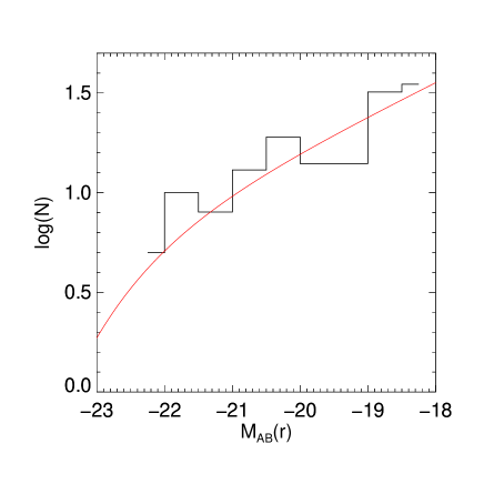
Figure 2: Left : $M_{AB}(r)$ histogram of the 150 galaxies in the local sample. The observed luminosity function from Blanton et al. (2003) is over-plotted in red. Right : $M_{AB}(r)$ histogram of the 150 galaxies in the distant sample with the observed red band luminosity function from Ilbert et al. (2005) shown as a red line.

2.3 Comparison between the SDSS and HST images

The aim is to classify the morphology of two galaxy samples that are representative of the same galaxy population at two different epochs. To avoid potential biases while comparing samples at different redshifts, it is important to make sure that the spatial resolution, depth, and rest-frame wavelengths sampled by all the images are similar.

The rest-frame wavelengths at which morphology is studied must be representative of galaxy mass, i.e., images in a photometric band that samples the galaxy spectrum $>$ 4000 Å  at rest are required. The SDSS $r$ band (with a central wavelength $\lambda_{c}=$ 6166 Å; see Sect. 2.2.1) from which the local sample was selected satisfies this requirement, and also presents the advantage to be redshifted into the HST $z$ band at $z\sim 0.5$.

The 0.1 arcsec PSF FWHM of the GOODS/ACS images corresponds to 0.63 kpc at the median $z=0.53$ of the distant sample, while the 1.4 arcsec PSF FWHM of the $r$-band SDSS images corresponds to 0.81 kpc at the median $z=0.029$ of the local sample, which implies that all the images sample similar spatial resolution. Moreover, the good agreement between the rest-frame bands sampled by the HST/ACS and the SDSS data (see Tab. 1) minimizes the $k$ correction between the two data sets. Finally, the depths of the two surveys can be compared using the ratio between the two signal-to-noise ratios that would be obtained if one would be observing the same source at $z=0$ from the SDSS and at $z=0.5$ from GOODS (see detailed calculation in App. A). The SDSS images are found to be deeper than the HST/ACS-GOODS images by 0.5, 0.8, and 0.6 magnitudes in the rest-frame $u$, $g$, and $r$ bands respectively.

Table 1: Wavelength comparison between different SDSS and HST/ACS bands. The rest-frame wavelengths are calculated assuming a redshift range [0.4-0.6].

Images		$u$	$g$	$r$	$i$	$z$
SDSS		3551Å	4686Å	6165Å	7481Å	8931Å
	$B$	$V$	$i$	$z$
HST/ACS	4312Å	5915Å	7697Å	9103Å
rest-frame	[2695-3080]Å	[3697-4225]Å	[4811-5498]Å	[5689-6502]Å

	SDSS			GOODS (ACS)
Telescope diameter $D$ (m)	2.5			2.4
Filter	$u$	$g$	$r$	$V$	$i$	$z$
Exposure time $T$ (s)	53.9	53.9	53.9	5450.0	7028.0	18232.0
Filter effective wavelength $\lambda$ (Å)	3551	4686	6166	5915	7697	9103
Filter width $\Delta\lambda$ (Å)	567	1387	1373	1565,5	1017,40	1269,10
Sky surface brightness	22.15	21.85	20.85	22.74	22.72	22.36

Table 2: Observational parameters for both SDSS and GOODS imaging.

3 Morphological analysis

The morphological classification of each galaxy relies on a process that was formalised in Delgado-Serrano et al. (2010) as a semi-automatic decision tree, which takes into account the well-known morphologies of local galaxies that populate the Hubble sequence. To minimize the remaining subjectivity, three of us (FH, HF, MP) independently classified each galaxy using this tree. The results were then compared and disagreement cases discussed until a final classification was agreed by all classifiers. The decision was based on the examination of the elements described below : a color map and the decomposition in several components of the light profile analysis in a single photometric band ($r$ band for the local sample and $z$ band for the distant one). We recall that as star formation likely affects the aspect of a galaxy in the rest-frame blue bands, the morphological classification must be performed in a (rest-frame) red band in which the emission is dominated by main sequence stars, which form the most part of the stellar mass, hence our choice for the working bands.

3.1 Color images and maps

Color information is essential to classify the morphology of a galaxy. A measure of the color in each pixel of the image offers the possibility to examine different galaxy components/regions separately and assess whether they correspond to simple star forming regions or are real sub-structures.

To do so, we subtracted pixel by pixel the magnitudes in two observed bands using a method that provides measurements of both the colors and the associated signal-to-noise ratios (see Zheng et al. 2005 for more details). Since all the considered bands have similar resolution and sampling, no PSF matching was needed so that the images were directly subtracted one from the other. The two bands used were $u-r$ for the local galaxies and $v-z$ for the distant ones, ensuring a meaningful comparison between the same rest-frame colors. For the distant sample we also used the $B-z$ color-map, because the $v-z$ color did not allow us to classify properly early-type galaxies at our working redshifts. Indeed, the rest-frame $V$ band corresponds to the Balmer break region, which can be affected by recent star formation. Such star formation bursts can occur in the central regions of a galaxy if some gas was captured 1 Gyr ago, which leads to a blue core in the $V-z$ color map compared to the rest of the galaxy. We observed this phenomenon especially in E and S0 galaxies, in which gas might be more likely prone to infalling motions towards the center, while in spiral galaxies the gas more likely follow circular trajectories along the disc. The $B-z$ color map was therefore used to distinguish between real blue cored galaxies and early-type galaxies that are only affected by this effect at their centers.

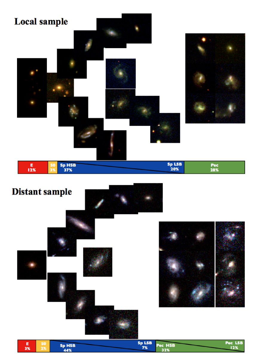
Figure 9: Present-day morphological sequence derived from the local sub-M* sample (top panel) and past morphological sequence derived from the distant sub-M* sample (bottom panel). Each stamp are 25 kpc wide and represents approximatively 5% of the galaxy population.

Three-band color images were also constructed using u-g-r bands for the local sample and V-i-z bands for the distant one, as those shown in Fig. 9.

For the distant sample, we also used infrared $J$ and $H$ HST/WFC3 CANDELS images (see Sect. 2.2.2), which were helpful to remove doubts when clumpy structures were visible in $z$ band, and distinguish between irregular galaxies and regular discs: as the infrared bands are more representative of the galaxy stellar mass, if such structures were also visible in $J$ and $H$, then they represented a non negligible part of the galaxy mass, and the galaxy was classified as irregular.

3.2 Light profile decomposition

The light profile of each galaxy was analysed in the rest-frame $r$ band, i.e., using the observed $r$ band for the local sample and the observed $z$ band for the distant sample.

First, the position angle and the axis ratio of the galaxy were measured using SExtractor. The half-light radius was then derived from the flux curve-of-growth constructed by measuring the flux in concentric ellipses of increasing radii. This curve reaches a plateau when the ellipses covers all the galaxy surface and start sampling the background. The half-light radius was estimated as the radius at which the measured flux equals half the total flux (measured on the curve-of-growth plateau). For both the local and distant samples, we checked that the positions of the galaxies in the $R_{half}$ vs. $M_{stellar}$ plane are consistent with the relations observed in large surveys (see e.g. Shen et al. 2003 and Dutton et al. 2011 and references therein).

The two-dimensional surface brightness distribution of each galaxy was fitted using GALFIT (Peng et al., 2002) using a linear combination of different components:

• A bulge, modelled by a Sersic (Sersic, 1968) profile

  $$\Sigma(r)=\Sigma_{e}e^{-\kappa_{n}[(r/r_{e})^{1/n}-1]},$$ (1)

  where $r_{e}$ is the effective radius enclosing half the total light, $\Sigma_{e}$ is the surface brightness at $r_{e}$, $n$ is the Sersic index, and $\kappa_{n}$ is a constant depending on $n$;

• A disc, modelled by an exponential profile

  $$\Sigma(r)=\Sigma_{0}e^{-r/r_{d}},$$ (2)

  where $\Sigma_{0}$ is the central surface brightness, and $r_{d}$ is the disc scale-length;

• If present a bar was added as an elongated (i.e., with a small $b/a$ axis ratio) Sersic component. When a bar was present but the resolution not sufficient to resolve it, the central Sersic component of the galaxy was considered to be the resulting superimposition of the bar and the bulge;

• The sky background was modelled as a constant with first-guess value estimated from the initial Sextractor analysis (see above). This component was let free during the fitting process.

The ratio between the bulge and the total flux ($B/T$) was estimated from this decomposition. Note that $B/T$ cannot be straightforwardly estimated from pre-calculated parameters such as the frac_deV quantity provided to the SDSS database (see App. C).

For each galaxy we used an iterative process to find the best decomposition model. First, a radial surface brightness profile in log stretch was constructed and carefully inspected for a change in slope, which evidences at least two components. A first-guess model was then constructed by fitting visually the two regions of the profile corresponding to the bulge and the disc, which was used as inputs for GALFIT. The residual image provided by GALFIT after it has converged from these initial conditions was visually inspected: if an elongated and symmetric central structure was identified, then a bar was added to the model and GALFIT run again using these new initial conditions. Note that for the smallest galaxies the spatial resolution and signal-to-noise ratio was not always sufficient to allow GALFIT to converge with three components, which sometimes resulted in a bar structure still visible in the residual map.

This iterative method was essential to make GALFIT converge towards the most meaningful solution. Indeed, the fitting process with GALFIT is based on a $\chi^{2}$ minimization using a Levenberg-Marquardt algorithm. This can efficiently finds a local minimum, which is not necessarily the global minimum. This makes GALFIT quite sensitive to the initial conditions and can result in GALFIT converging towards a solution that has no physical meaning, even if the $\chi^{2}$ is minimized to a reasonable value. Degeneracies occur especially when fitting multi-component models with a large number of free parameters to faint and distant galaxies that are poorly resolved or have a low signal-to-noise ratio. Note that in some extreme cases of degeneracies some parameters had to be constrained to a range of values or even to be fixed to reduce the parameter space to be explored.

3.3 Morphological classification

Taking into account the color maps, the color images, the models produced by GALFIT, and especially the residual maps (subtraction between the initial image and the model), each galaxy was classified into the following morphological classes:

• Elliptical galaxies (E) must show a prominent bulge with B/T ranging between 0.8 and 1, and an overall red color;

• Lenticular galaxies (S0) must also show a prominent bulge with B/T ranging between 0.5 and 0.8; this bulge is required to be redder than the underlying disc. The disc must be highly symmetric with no signs of regular structure such as arms;

• Spiral galaxies (Sp) must show both a bulge and a disc, or a single, pure exponential disc. The B/T ratio must range between 0 and 0.5, and the bulge, if present, must be redder than the disc. The disc must be symmetric but can present regular structures such as spiral arms, which can be identified in the residual map provided by GALFIT. A central bar can also be present as an elongated Sersic profile;

• Peculiar galaxies (Pec) must show asymmetrical features, which can be identified in the residual map. Irregularities associated to strong color gradients were assumed to be due to merger events (Pec/M). Galaxies with very asymmetrical tidal features were associated to merger remnant (Pec/MR). Tadpole-like (Pec/Tad) galaxies must show a bright knot associated to an extended tail. Irregular galaxies (Pec/Irr) must show only an asymmetric light profile, or two off-centered components. Galaxies with a bulge bluer than the disc (by more than $\sim$0.2 mag) were also classified as peculiar because of their unexpected blue nucleus (Pec/BNG). Galaxies with a half-light radius smaller than 1 kpc were classified as compact galaxies (Pec/C).

4 Low surface brightness galaxies

4.1 Defining LSB galaxies

For historical reasons Low Surface Brightness galaxies (LSBs) were often defined as galaxies dominated by an exponential disc with a $B$-band central surface brightness fainter than 22 mag.arcsec^-2. This limit was first determined from a sample of 36 spiral galaxies studied by Freeman (1970), adopting a 1$\sigma$ threshold fainter than the peak of the distribution of their extrapolated disc central surface brightness. However, this narrow surface brightness distribution was shown to be due to selection effects (Disney 1976) that act against the detection of galaxies fainter than the sky brightness (see also Sect. 6.1.3). LSB galaxies were extensively studied in the local Universe selected on the basis of their blue central surface brightness.

However, because the blue band is very sensitive to star formation, which was more intense in the past, the blue central surface brightness distribution of galaxies is found to shift towards brighter magnitudes with increasing redshift (see, e.g., Schade et al. 1995 who found a strong evolution of 1.2 mag in the rest-frame B-band central surface brightness distribution of galaxies at $z>0.5$). It is therefore important to define LSB galaxies with a criterion that is not biased by stellar evolution when applying it at different redshifts. We chose to define LSB galaxies in both the local and distant samples as galaxies with a disc central surface brightness at least 1$\sigma$ fainter than the median rest-frame $r$-band central surface brightness in a given sample.

4.2 Disc central surface brightness distribution

In this section, only galaxies with a non negligible disc component (i.e., S0 and spiral galaxies, as well as peculiar galaxies for which the light profile reveals a disc component) are considered. The measurement of the central surface brightness in highly inclined galaxies is affected by two competing effects: the more inclined a disc galaxy is, the larger the integrated stellar light is along the line of sight and the larger dust extinction effects are. To circumvent this, we restricted the study of LSB galaxies to galaxies with an axis ratio $b/a\geq 0.5$, which corresponds approximately to an inclination smaller than 60$\degree$. This resulted in sub-samples of 68 local disc galaxies and 78 distant disc galaxies. We checked that these two sub-samples are still representative of their parent samples, as evidenced by Kolmogorov-Smirnov tests (which resulted in probabilities of 97% and 96% that the local and distant sub-samples and the luminosity function at the corresponding redshifts are drawn from the same parent distributions).

Assuming an infinitely thin disc, integration of Eq. 2 gives the total flux of the disc component:

$$F_{tot}=2\pi r_{d}^{2}\Sigma_{0},$$ (3)

where $r_{d}$ is the disc scale-length (in arcsec), and $\Sigma_{0}$ the central surface brightness as defined by Eq 2. By converting this in logarithmic scale and including the correction for extinction and cosmological dimming effects, one gets the following relation to estimate the disc central surface brightness in a given photometric band:

$$\mu_{0}=m_{d}+2.5\log(2\pi r_{d}^{2})-10\log(1+z)-A_{\lambda},$$ (4)

where $m_{d}$ refers to the total magnitude of the disc, $z$ is the redshift, and $A_{\lambda}$ is the galactic extinction. $m_{d}$ and $r_{d}$ were both estimated by GALFIT when fitting the galaxy profile. For local galaxies, the galactic extinction, calculated following Schlegel, Finkbeiner & Davis (1998) was taken from the SDSS database. For distant galaxies, which are observed far from the galactic plane, this correction can be neglected.

The resulting disc central surface brightness distributions in the local and distant samples are shown in Fig 3. The median surface brightnesses in both samples were found to be $\mu_{0}(r)$=20.7 mag.arcsec^-2 and 20.2 mag.arcsec^-2 for the local and distant samples respectively, with a standard deviation of 1 mag.arcsec^-2 for both. The median shift of 0.5 mag between the two distributions is consistent with expectations from a pure passive stellar evolution over 5 billion years (e.g., Charlot, Worthey & Bressan 1996). As stated above, we therefore defined LSB galaxies as galaxies with a disc central surface brightness at least 1$\sigma$ fainter than the above median value, i.e., $\mu_{0}(r)\geq$ 21.7 mag.arcsec^-2 for local galaxies and $\geq$ 21.2 mag.arcsec^-2 for distant galaxies.

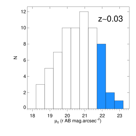
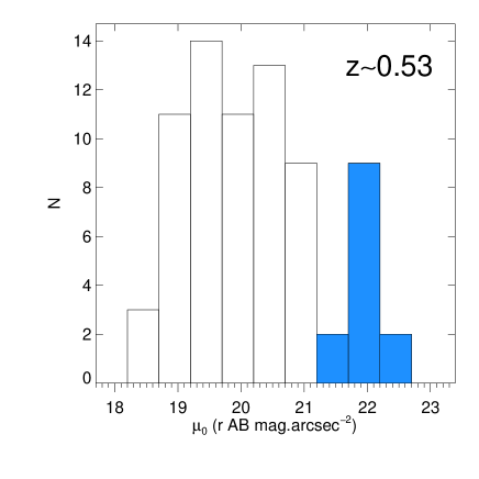
Figure 3: Disc central surface brightness distribution for local (left panel) and distant (right panel) galaxies in the rest-frame SDSS $r$ band. Median values are 20.7 and 20.2 mag.arcsec^-2 for the local and distant samples respectively, with a standard deviation of 1 mag.arcsec^-2 for both. Defining LSBs as disc galaxies with a disc central surface brightness at least 1$\sigma$ above the median value, the bins corresponding to LSBs are shown in blue.

4.3 A new class of Giant LSB discs at $z\sim 0.5$

Figure 4 shows the disc scale-lengths derived from the GALFIT 2D fitting as a function of the $r$-band absolute magnitudes for both the local and distant low-inclination disc galaxies sub-samples. For both the local and distant samples, the disc scale-length decreases with absolute magnitude as expected from Eq. 4, evidencing that the decompositions led to robust disc components that follow the Freeman’s law. By contrast, low surface brightness galaxies (blue symbols) are clearly shifted upward, i.e., they have larger disc scale-lengths compared to high surface brightness galaxies of similar mass. In the local sample, 80% of the LSB galaxies are found to be bulgeless spiral galaxies, half of which show a bar.

In the distant sample, 60% of the LSB galaxies were classified as Pec/Irr galaxies because they reveal very disturbed morphologies with asymmetrical brightness profiles and clumps. Their GALFIT model comprises two components: a Sersic profile with $n\sim 1$ in the inner component and an extended exponential LSB disc. Comparing the local and distant samples reveals a population of distant galaxies with small stellar masses ($M_{AB}(r)>-19$) and very extended LSB discs ($r_{d}\geq 4-5$ kpc), which appear not to exist at lower redshifts. The scale-length of these discs are comparable to those of more massive high surface brightness spiral galaxies, e.g., M31 was found to have $r_{d}=5.9\pm 0.3$ kpc in $R$ band (Hammer et al., 2007). Figure 5 shows four of these giant LSB discs ($r_{d}>5$ kpc) found in galaxies with stellar masses close to that of the LMC. Such extended LSB discs are further discussed in Sect. 6.1.3.

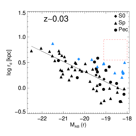
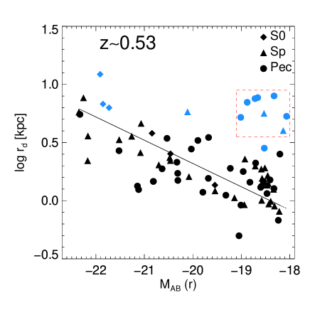
Figure 4: Relation between disc scale-lengths $r_{d}$ and luminosities in $r$ band for disc galaxies with $i\leq 60\degree$, at low (left) and high (right) redshifts. The plot at high redshifts shows a population of giant LSB discs with $r_{d}\geq 3-4$ kpc and with low luminosities (see the region ensquared in dashed red), which appears not to exist at low redshifts. The black line represents how $\mu_{0}(r)$ is expected to decrease with $m_{d}$ from Eq. 4 with $\mu_{0}(r)$=20.7 mag.arcsec^-2, i.e., the median local $\mu_{0}(r)$).

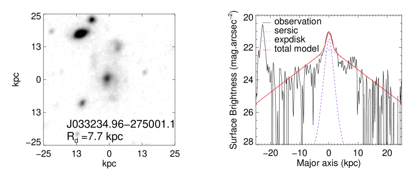
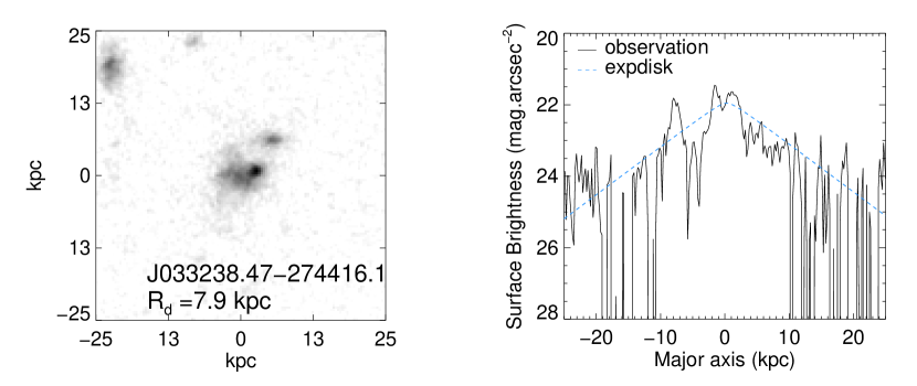
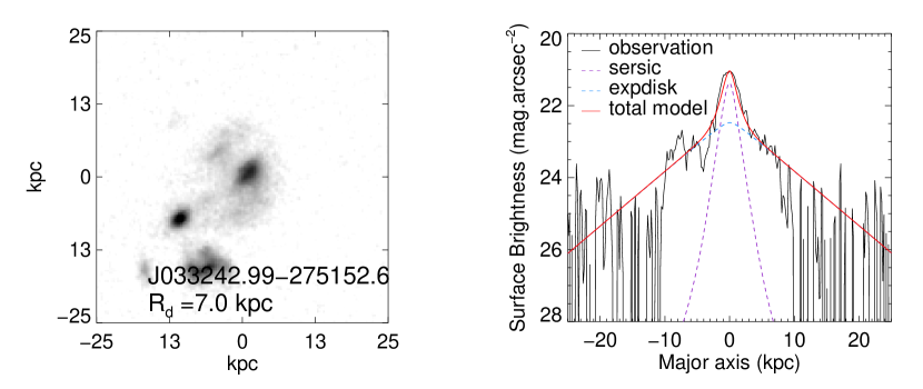
Figure 5: Examples of the most extreme LSB galaxies at z $\sim$ 0.5. The left panels show the summed $i+z+J+H$ images of the galaxies (ACS $i$ and $z$ images were rescaled to the WFC3 resolution). The right panels show the observed profile along the major axis of the galaxy disc (black line). The profile of the model that has been fitted is superimposed in red. When the model comprises several components, the profile of each sub-component is shown. Because of the very low signal-to-noise ratio of the disc, GALFIT tends to underestimate the disc size. We thus kept the disc scale-length parameter fixed during the process : we fitted it by visual inspection so that the model profile follows the disc wings at best.

5 Building up a morphological sequence of low mass galaxies

Table 3 summarizes the fraction of E, S0, spiral (Sp) and peculiar (Pec) galaxies that were found in two mass ranges, i.e., $M_{stellar}<1.5\times 10^{10}$ $M_{\odot}$ (low mass or sub-M* range) and $M_{stellar}\geq 1.5\times 10^{10}$ $M_{\odot}$ (high mass range). This limit corresponds to $M_{AB}(r)\sim-20$.

5.1 High mass sub-samples and comparison with previous studies

A fraction of 81-15-5% of the local massive galaxy population is found to be Sp-E/S0-Pec galaxies, respectively. At high redshift we find a slight increase of the fraction of E/S0 and Pec, but a dramatic decrease of the fraction of Sp. These results can be directly compared to Delgado-Serrano et al. (2010), who selected galaxies with $M_{J}\leq-20.3$, which also corresponds to $M_{stellar}\geq 1.5\times 10^{10}M_{\odot}$. Our results are found to be consistent, which confirms the evolution of the fraction of Pec and Sp galaxies with redshift, suggesting that peculiar galaxies transform into spirals. Nevertheless, we find a less dramatic quantitative evolution: in our distant high mass galaxy sample, the fraction of spirals remains higher than the fraction of peculiar galaxies (45% and 27% of spirals and peculiar respectively instead of 31% and 52% in the sample of Delgado-Serrano et al. 2010). These differences could also be explained by the fact that we probe a slightly more recent epoch of the Universe compared to them (the median redshift of our distant sample is $z=0.53$ instead of $z=0.65$ in their sample). Moreover, while they found no evolution in the fraction of E/S0 galaxies, we find a slight increase with redshift, which is not so significantly when accounting for the relatively large statistical uncertainties due to the limited sample sizes. The consistency between our results and previous works strengthens the robustness of our classification process.

5.2 Morphological classification of the low mass subsamples

We built two morphological sequences of low-mass galaxies at $z\sim 0$ and $z\sim 0.53$, which are shown in Fig. 9. Each stamp in these figures represents approximately 5% of the galaxies in the sample. The counting of bars and LSB galaxies is performed in the sub-samples of galaxies restricted to $b/a\geq 0.5$ because of possible biases due to inclination and dust on the bar detection as well as on the central surface brightness calculation (see Sect. 4.2).

5.2.1 Local low-mass galaxies

The local low-mass galaxy population consists in 15% of E/S0, 57% of Sp, and 28% of Pec galaxies (see Tab. 3). The major difference with the higher mass galaxy sample is the fraction of peculiar galaxies in the local Universe, which represents one third of the local low-mass galaxy population instead of only a few percents in the well-known Hubble sequence. The fraction of E/S0 is comparable to what was found for high-mass galaxies. The population of spiral galaxies represents slightly more than half of the local galaxies compared to more than 75% for high-mass galaxies. They mainly consists in bulgeless galaxies (less than 10% of the spirals have B/T $>$ 0.2). LSB galaxies, as defined in the previous section, represent about 20% of the local galaxy population in this range of mass (and one third of the spiral galaxies). They are found to be almost exclusively spiral galaxies, most of them showing a prominent bar.

5.2.2 Distant low-mass galaxies

We find that the distant population of low-mass galaxies consists of 5% of E/S0, 51% of Sp, and 44% of Pec galaxies. The fraction of early-type galaxies is a factor three smaller compared to the local sample. The fraction of Sp galaxies shows no evolution, in stark contradiction with high-mass galaxies. They all have B/T $<$ 0.1, and only 10% of them that are found to be LSBs. The fraction of Pec galaxies is larger compared to the local sample. This increase can be ascribed to the giant and irregular LSB discs that are not detected in the local Universe (see Sect. 4.3).

Table 3: Number of galaxies in each morphological class and corresponding fractions for local and distant samples. LSB and HSB fractions were calculated in the subsamples of low-inclination galaxies (with $b/a\geq 0.5$). Uncertainties given in parentheses were calculated assuming Poisson statistics, as $\sqrt{N}/N$.

	$M_{stellar}<1.5.10^{10}M_{\odot}$				$M_{stellar}\geq 1.5.10^{10}M_{\odot}$
	Local		Distant		Local		Distant
E	11	(12$\pm$4 %)	3	(3$\pm$2 %)	3	(5$\pm$3 %)	6	(12$\pm$5 %)
S0	2	(2$\pm$1 %)	2	(2$\pm$1 %)	6	(10$\pm$4 %)	8	(16$\pm$6 %)
Sp	52	(58$\pm$8 %)	50	(51$\pm$7 %)	48	(81$\pm$12 %)	23	(45$\pm$9 %)
HSB		39$\pm$7 %		44$\pm$7 %
LSB		19$\pm$5 %		7$\pm$3 %
Pec	25	(28$\pm$6 %)	44	(44$\pm$7 %)	2	(4$\pm$2 %)	14	(27$\pm$7 %)
HSB		26$\pm$5 %		33$\pm$6 %
LSB		2$\pm$1 %		11$\pm$3 %
Total	90	(100%)	99	(100%)	59	(100%)	51	(100%)
Disc galaxies :
without bulge		62$\pm$ 8%		71$\pm$ 8%		8$\pm$ 4%		21$\pm$ 7%
with pseudo bulges ($n<2$)		16$\pm$ 4%		19$\pm$ 4%		46$\pm$ 9%		43$\pm$ 9%
with classical bulges ($n\geq 2$)		8$\pm$ 3%		5$\pm$ 2%		31$\pm$ 7%		8$\pm$ 4%

6 Discussion

6.1 Potential limitations of the study

6.1.1 Photometric redshifts

One of the main limitation of the study may be linked to the use of photometric redshifts to build the distant sample of galaxies. We indeed first tried to use the ESO-GOODS spectroscopic master catalogue gathering all publicly available redshifts in the CDFS but it did not allow us to build a complete volume-limited sample down to $M_{AB}(r)=-18$ at such redshifts. Sampling such small masses is only currently possible using photometric redshift estimates. The catalogue of Dahlen et al. (2010) provides us with the best photometric redshift estimates so far, with a scatter in $\Delta z/(1+z_{spec})$ of only 0.04 between the spectroscopic redshifts they retrieved and their photometric estimates.

We have also cross-correlated the photometric redshift catalogue with the ESO spectroscopic catalogue to evaluate how errors in redshifts could affect the sample selection. We have considered only the most secure redshifts both in the spectroscopic catalogue, in which redshifts are provided with a quality flag, and in the photometric catalogue from which we kept only redshifts that were estimated using at least ten photometric bands. We then fitted the $\Delta z/(1+z_{spec})$ distribution by a Gaussian and found $\sigma=0.033$. The comparison between spectroscopic and photometric redshifts is shown in Fig.6. Since the scatter is much smaller than our working redshift range, we do not expect possible redshift errors to affect significantly the sample selection.

Another issue to be considered is the effect of catastrophic failures: we found that 12% of objects have $\Delta z/(1+z_{spec})>0.1$, which would represent two stamps in our sequence (Fig. 9). Furthermore, Fig. 2 shows that the distant sample follows the same logN-logS behavior that the Ilbert et al. (2005) counts, which are based on spectroscopic redshifts. It indicates that a similar number of objects near the sample limits (in redshift or in absolute magnitude) are included/excluded because of photometric redshifts uncertainties. We conclude that this effect cannot affect significantly the results.

Errors in photometric redshift estimates could also have an impact on surface brightness estimates, because of the cosmological dimming correction that varies as $(1+z)^{4}$. Indeed, an error of 0.033 in the redshift estimation leads to an error of 0.10 mag.arcsec^-2 at $z=0.5$ in surface brightness. This may affect the results on LSB galaxies and surface brightness evolution. We were able to retrieve spectroscopic redshifts for two of the large LSB discs: their photometric redshifts were found to be 0.462 for both while the spectroscopy confirms them at 0.503 (J033242.99-275152.6) and at 0.523 (J033225.07-274605.8), respectively. The first (second) galaxy would have $\mu_{0}(r)$ = 22.52 (21.80) mag.arcsec^-2 instead of 22.64 (21.98) mag.arcsec^-2, implying that their LSB nature remains unchanged. It illustrates again that the results might be affected by uncertainties associated to photometric redshifts only in a marginal way, i.e., only for galaxies near the adopted limits.

Figure 6: Comparison between spectroscopic redshifts (from the ESO master spectroscopic catalogue) and photometric redshifts (from Dahlen et al. 2010). Fitting $\Delta z/(1+z_{spec})$ by a Gaussian, the scatter is found to be $\sigma=0.033$. Red points represent cases of catastrophic failure, defined as $\Delta z/(1+z_{spec})>0.1$.

6.1.2 Uncertainties on mass estimates

Mass estimation is still a major issue in extragalactic studies. Stellar mass estimates are subject to systematic uncertainties related to the choice of the IMF and the star formation history (see, e.g., the discussion in Bell et al. 2003). Fig. 7 evidences a significant excess of low mass galaxies concentrating near log($M_{stellar}/M_{\odot}$)=9.5 when comparing the distant and the local sample. This results from an evolution of the number density of low mass galaxies during the last 5 Gyr, as evidenced by the comparison between the local and distant luminosity functions shown in Fig. 2 (see also Introduction). Stellar masses were derived in a very similar way for both samples and we verified that errors due to photometric redshifts cannot affect significantly these estimates.

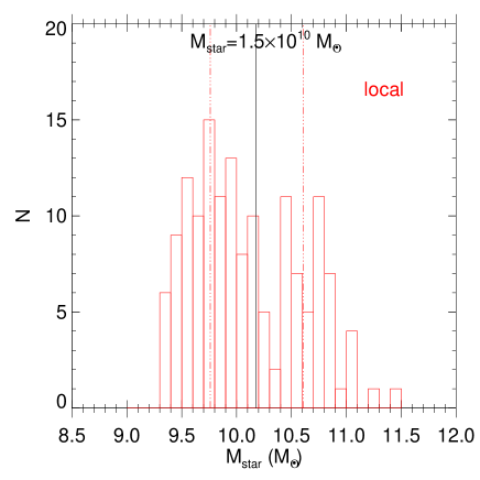
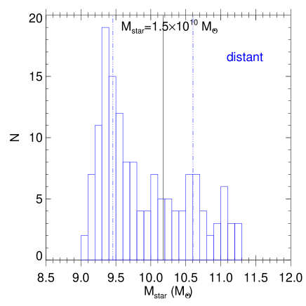
Figure 7: Histograms of stellar masses for the local (left) and distant (right) samples. Vertical dotted lines represent the median mass values for the lower ($M_{stellar}<1.5\times 10^{10}$ $M_{\odot}$) and upper ($M_{stellar}>1.5\times 10^{10}$ $M_{\odot}$) mass sub-samples.

6.1.3 Could we have missed very low SB galaxies?

Samples of galaxies with small stellar masses can be affected by the limits in surface brightness detection. Figure 3 (left panel) shows a significant drop of the local galaxy counts above $\mu_{0}(r)\sim 22.5$ mag.arcsec^-2. Accounting for Eq. 4 and the adopted absolute magnitude limit ($M_{AB}(r)<-18$), this suggests that LSB galaxies with a disc scale-length larger than 2.5 kpc may be underrepresented/missing in the samples. In particular, comparing the two panels of Fig. 4, one can see that there are several distant LSBs in the interval $M_{AB}(r)=$-18 to -19 with scale-lengths larger than 3.5 kpc, but none in the local sample (see the red box in Fig. 4).

We show in App. A that the SDSS images are expected to be a factor $\sim$ 1.5-2.6 deeper than the HST/GOODS images when considering the $S/N$ obtained per constant 1 $kpc^{2}$ apertures and/or per pixels. This suggests that it is unlikely that LSB galaxies were missed in the local sample because of an insufficient depth compared to the high-z sample. To investigate this further, we simulated fake SDSS and HST images of giant LSBs and we then tried to recover their morphological parameters with GALFIT using exactly the same procedure that the one used for observed galaxies (see Sect. 3.2). These simulations reveal that extended LSB discs can be well identified in both samples (see details in App. B). This strengthens the calculation of App. A and reveals that possible uncertainties in the fitting procedure, e.g., background subtraction, are not severally limiting the detection of giant LSB in both samples.

Comparing the two panels in Fig. 4, we find no giant LSB among 17 galaxies between $-19<M_{AB}(r)<-18$ in the local sample, while 8 giant LSBs among 35 such galaxies are found in the distant sample ($\sim$ 23%, i.e., those in the red box in Fig. 4). Assuming that the fraction of giant LSBs does not evolve with redshift, one would expect from the distant sample that the number of local giant LSBs is 4. Since the corresponding Poisson uncertainty is $\sqrt{4}=2$, the reported evolution of giant LSBs is however only a $\sim$ 2 $\sigma$ effect within the studied local sample. To check whether this can be due to Poisson fluctuations, we selected 70 additional SDSS galaxies between $-19<M_{AB}(r)<-18$ to obtain a sample of 120 local galaxies in this range of luminosity. We then decomposed their light distribution, constructed color maps and images, and classified their morphologically, following the method described in Sect. 3 and Sect. 4.2 (i.e., we kept only disc-dominated galaxies with $b/a>0.5$ to limit effects due to inclination). These new galaxies were added to the $R_{d}$ vs. $M_{AB}(r)$ plot as open green symbols, as show in Fig. 8. This test reveals only one possible giant LSB (with Pec morphology) in the local sample. We can therefore conclude that the evolution of the fraction of giant LSBs is at least a 4.4 $\sigma$ effect.

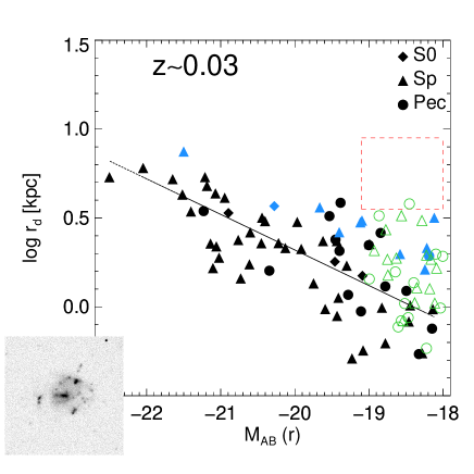
Figure 8: Same as Fig. 4 but including an additional sample of 70 galaxies between $-19<M_{AB}(r)<-18$ shown as open green symbols. The stamp image on the lower-left corner shows the summed g+r+i+z image of the only one large LSB found in the additional sample (corresponding to the open green symbol in the red box).

6.2 Evolutionary link between the local and distant sequences of low-mass galaxies

Delgado-Serrano et al. (2010) succeeded to build two Hubble Sequences for distant and nearby galaxies and to establish a causal link between them. It has revealed a considerable evolution of Sp galaxies, whose progenitors are mostly Pec galaxies. This is corroborated by their internal motions revealed by 3D spectroscopy (Neichel et al., 2008), and then interpreted and modelled as being the result of gas-rich major mergers at various phases $\sim$ 6 Gyr ago (Hammer et al., 2009). Within the limitations discussed in Sect. 6.1, Fig. 9 provides the first ever made attempt to link the populations of sub-M* galaxies over an elapsed time of $\sim$ 5 Gyr.

Assuming that morphological peculiarities are associated to merger events, one can check the consistency of the fraction of Pec galaxies with the fraction of mergers expected at the two epochs sampled by the local and distant samples. For this, we used the merger rates derived by Puech et al. (2012) using the semi-empirical model introduced by Hopkins et al. (2010b). The fraction of major mergers (defined as stellar mass ratios $\leq$ 4:1) for events involving galaxies with stellar mass similar to that of the high-mass samples is expected to be $\sim$11% and $\sim$30% at $z=0$ and $z\sim 0.5$ respectively. This assumes that the morphological classification can identify Pec/major mergers during a total visibility timescale of 3.2 Gyr. Note that parametric morphological classifications can generally detect only galaxies during the fusion phase (and partly during the pre-fusion phase with a total visibility timescale $<$1.5 Gyr, see, e.g., Lotz et al. 2010), while our morphological classification method allows detecting mergers both in the pre-fusion and fusion phases, which are both found to last $\sim$1.8 Gyr (see Fig. 8 of Puech et al. 2012) for galaxies in this range of mass. We corrected the total pre-fusion + fusion timescale for the phases during which galaxies would appear as relatively separated pairs with limited morphological perturbances, which led us to adopting a total visibility timescale $\sim$ 3.2 Gyr. These fractions can naturally account for the fraction of Pec galaxies found in both the local and distant high-mass samples (see Tab. 3) with no need of invoking any other processes.

For sub-M* galaxy mergers, the dynamical timescale for two galaxies to merger is expected to be longer by a factor $M_{stellar}^{-1/4}$. Since the amplitude of the morphological disturbances depends mainly on the mass ratio of the merger, it is therefore expected that the total timescale over which major mergers between sub-M* galaxies can be identified will be at first order a factor $M_{stellar}^{-1/4}$ (i.e., $\sim$80%) longer compared to super-M* mergers with same mass ratios. The fraction of expected major mergers is then found to be $\sim$8% and $\sim$31% in the local and distant sub-M* samples respectively. There are therefore not enough major mergers occurring in this range of mass to account for all Pec low-mass galaxies (28% and 44% in the local and distant samples respectively, see Tab. 3). Accounting for more minor mergers (i.e., accounting for stellar mass ratios down to 10:1 instead of 4:1) the fraction of galaxies expected to be involved in major+minor mergers is found to be 13% and 49% at $z=0$ and $z\sim 0.5$, respectively, which better accounts for the fraction of low-mass Pec galaxies, especially at high redshifts. Such an increasing role of minor mergers in the evolution of sub-M* galaxies is indeed consistent with expectations from more refined semi-empirical models (Hopkins et al., 2010a). It is also consistent with the prevalence of pure discs and pseudo-bulges amongst low-mass galaxies: 78 and 90% of low-mass galaxies are indeed found to have pseudo-bulges (i.e. with a Sersic index $n<2$, see Fisher & Drory 2008) or to be bulgeless galaxies in the local and distant samples, respectively (see Tab. 3).

The 12% of the low-mass distant galaxies that have extended LSB discs show strongly perturbed morphologies (see, e.g., Fig. 5), which suggest past interactions and contrast with the finding that LSB discs generally do not show evidence for star formation (e.g., van der Hulst et al. 1993, van den Hoek et al. 2000, Boissier et al. 2008). They are also found to be relatively clumpy, which might also suggest disc instabilities as suggested by Kassin et al. (2012). Interestingly, Guo et al. (2015) found that minor mergers are a viable explanation for the observed redshift evolution of the fraction of clumps out to z$\sim$1.5. Their large extent may share some resemblance with the giant LSB galaxies (GLSB) that were discovered in the local Universe (Sprayberry et al. 1995 ; Barth 2007 ; Kasparova et al. 2014), such as Malin 2. However the distant LSB discs in this paper have scale-lengths ranging from 3 to 8 kpc, instead of 19 kpc for Malin 2 (Kasparova et al., 2014). Mapelli et al. (2008) suggested that GLSB galaxies could form after a very efficient collision event, which would first produce a ring galaxy that further evolves into a GLSB galaxy. Such extreme processes are expected to be very rare because of the required very small impact parameters. Those are probably not necessary to explain the distant LSBs found in this paper, though merger/collision events are suggested from the images. 3D spectroscopy will be necessary to confirm (or infirm) that major and minor mergers prevail in the evolution of sub-M* galaxies, including in LSBs.

7 Conclusion

Sub-M* galaxies are a very numerous and evolving population, which may account for a significant part of the star formation density and its evolution. We have studied in detail two samples of galaxies, which are representative of the present-day galaxies and their progenitors, 5 Gyr ago. Our analysis is based on a full control of possible biases, including those related to surface brightness effects. We have analysed the galaxies 2D luminosity profiles and carefully decomposed them into bulges, bars, and discs. This was done in a very consistent way at the two epochs, by relying on the same image quality and (rest-frame red) filters. Using the morphological decision tree introduced by Delgado-Serrano et al. (2010), we have classified them into elliptical, lenticular, spiral, and peculiar galaxies.

We have discovered that at $z=0$, both massive and sub-M* galaxies follow similar Hubble Sequences, with a considerable larger number of peculiar galaxies in sub-M* galaxies. We also found in this range of mass an emergence of low surface brightness galaxies, which are mostly found to be disc galaxies. These trends persist in $z\sim 0.5$ galaxies, which suggests that sub-M* galaxies have not reached yet a virialised stage, conversely to their more massive counterparts. The fraction of distant peculiar galaxies is always high (27-44%), consistent with a hierarchical scenario in which minor mergers could have played a more important role than for more massive galaxies.

We also report the first discovery of a population of giant low surface brightness galaxies at $z=0.5$, which accounts for 5% (12%) of the overall galaxy (sub-M*) population at z=0.5. These galaxies are quite enigmatic because their disc scale-lengths are comparable to that of M31 while their stellar masses are closer to that of the LMC. Spatially-resolved spectroscopy as well as investigations of the neutral and ionized gas would be invaluable to establish more firmly the link between sub-M* galaxies at various epochs and investigate further the nature of the distant giant LSB discs.

Appendix A S/N of the SDSS and HST images

In this Appendix, we compare the signal-to-noise ratio ($S/N$) obtained in the SDSS and HST/ACS-GOODS images. Since the goal is to compare the overall morphology of galaxies at different redshifts, we first compare the $S/N$ expected in apertures of constant physical size. We chose apertures $A$ of size 1 $kpc^{2}$, which correspond to 2.96 $arcsec^{2}$ at $z_{SDSS}\sim 0.029$ and to 0.025 $arcsec^{2}$ at $z_{HST}\sim 0.53$ (see Sect. 2.3).

The S/N obtained within the area $A$ can be written as follows:

$$S/N=\frac{N^{source}}{\sqrt{N^{source}+ron^{2}\times N_{pix}+N^{bkg}}},$$ (5)

where $N^{source}$ is the number of detected photons from the source within $A$, $N^{bkg}$ is the corresponding number of photon from the background (e.g., sky), $ron$ is the detector read-out noise, and $N_{pix}$ is the number of detector pixels within $A$. Eq. 5 assumes that there are no residual signals from the data reduction. The galaxies were all observed in background-limited conditions in all bands except perhaps for the SDSS $u$-band images, for which galaxies were only on average $\sim$0.25 $mag.arcsec^{-2}$ fainter than the sky background (see Tab. 4). For simplicity, we assume that all galaxies were observed well in a background-limited regime, which implies that the above formula can be simplified as:

Table 4: Mean surface brightness of the galaxies within the optical radius $R_{opt}\sim 2\times R_{half}$. Galaxies are significantly fainter than the sky or zodiacal background surface brightness in all bands (except for the SDSS $u$ band, see Tab. 2).

	SDSS	HST/GOODS
Median observed total mag	16.1	22.9
Median observed $R_{half}$ (arcsec)	5.0	0.5
$\mu_{opt}$ (mag/arcsec2)	22.4	24.1

$$S/N\sim\frac{N^{source}}{\sqrt{N^{bkg}}}$$ (6)

The number of photons from the source detected within $A$ can be derived from the spectral density of the source surface brightness $SB_{\nu}^{source}$ (in $erg.s^{-1}.cm^{-2}.Hz^{-1}.arcsec^{-2}$) as follows:

$$N^{source}=SB_{\nu}^{source}\times\Delta\nu\times A\times S\times T_{exp}\times\frac{1}{h\nu_{c}}\times tr,$$ (7)

in which $\nu_{c}$ is the filter central frequency (in $Hz$), $h\nu_{c}$ represents the energy (in $erg$) per detected photon, the exposure time is $T_{exp}$ (in $s$), the collecting surface area is $S=\pi D_{tel}^{2}/4$ (where $D_{tel}$ is the telescope diameter in $cm$), $\Delta\nu$ is the filter width (in $Hz$), and $tr$ and the system global transmission. The source surface brightness spectral density and the $AB$ surface brightness are simply related by $\mu_{AB}^{source}=-2.5\times\log_{10}{(SB_{\nu}^{source})}-48.60$ so that the integrated $AB$ magnitude of the source is $m_{AB}=-2.5\times\log_{10}{(f_{\nu}^{source})}-48.60$ with $f_{\nu}\sim SB_{\nu}\times\pi(2.R_{half})^{2}/4$, in which $R_{half}$ is the source half-light radius (in $arcsec$) in the considered band.

Similarly, the number of photons from the dominating source of background light (i.e., the atmospheric sky background for SDSS images, and the zodiacal light for HST images) detected within $A$ can be derived from the spectral density of the background surface brightness $SB_{\nu}^{bkg}$ as follows:

$$N_{bkg}=SB_{\nu}^{bkg}\times\Delta\nu\times A\times S\times T_{exp}\times\frac{1}{h\nu_{c}}\times tr,$$ (8)

and then $\mu_{AB}^{bkg}=-2.5\times\log_{10}{(SB_{\nu}^{bkg})}-48.60$ is the $AB$ background surface brightness in magnitude scale.

The $S/N$ obtained within $A$ can be obtained by substituting Eqs. 7, and 8 in Eq. 6, which leads to:

$$S/N\sim\sqrt{\frac{\pi}{4h}}\times\sqrt{\frac{\Delta\nu}{\nu_{c}}}\times\sqrt{T_{exp}}\times D_{tel}\times\sqrt{A}\times\\ \sqrt{tr}\times\frac{SB_{\nu}^{source}}{\sqrt{SB_{\nu}^{bkg}}}$$ (9)

We now compare the $S/N$ that would be obtained if the same source was observed at $z=0$ and $z=0.53$ using two SDSS and HST/ACS filters. The ratio between the two $S/N$ is then:

$$\frac{S/N^{HST}}{S/N^{SDSS}}=\sqrt{\frac{\Delta\nu^{HST}}{\Delta\nu^{SDSS}}\times\frac{\nu^{SDSS}}{\nu^{HST}}\times\frac{T_{exp}^{HST}}{T_{exp}^{SDSS}}\times\frac{tr_{HST}}{tr_{SDSS}}}\\ \times\frac{D_{tel}^{HST}}{D_{tel}^{SDSS}}\times\sqrt{\frac{A^{HST}}{A^{SDSS}}}\times\frac{SB_{\nu}^{source,HST}}{SB_{\nu}^{source,SDSS}}\times\sqrt{\frac{SB_{\nu}^{bkg,SDSS}}{SB_{\nu}^{bkg,HST}}}$$ (10)

Redshifts and filters were chosen so that the observed HST/ACS filter for galaxies at $z\sim 0.53$ and the SDSS filter for galaxies at $z\sim 0$ sample similar rest-frame frequencies (see Sect. 2). For simplicity, we assume that the match in frequency is perfect so that the two central frequencies and the two filter widths verify the following relations:

$$\nu_{c}^{HST}=\frac{\nu_{c}^{SDSS}}{1+z},$$ (11)

$$\Delta\nu^{HST}=\frac{\Delta\nu^{SDSS}}{1+z}.$$ (12)

Finally, one has to account for cosmological dimming that decreases the source flux as $(1+z)^{4}$ and energy conservation (i.e., $SB_{\nu}\times\nu_{c}=$ cste) that implies $SB_{\nu}^{HST}=SB_{\nu}^{SDSS}\times(1+z)$, which both lead to:

$$SB_{\nu}^{HST}=\frac{SB_{\nu}^{SDSS}}{(1+z_{HST})^{3}}.$$ (13)

For simplicity, we assume here that $z_{SDSS}=0$ for the local galaxy sample.

Injecting these last three equations into Eq. 10 yields the following relation:

$$\frac{S/N^{HST}}{S/N^{SDSS}}=\sqrt{\frac{T_{exp}^{HST}}{T_{exp}^{SDSS}}\times\frac{tr_{HST}}{tr_{SDSS}}}\times\frac{D_{tel}^{HST}}{D_{tel}^{SDSS}}\times\sqrt{\frac{A^{HST}}{A^{SDSS}}}\\ \times\frac{1}{(1+z_{HST})^{3}}\times\sqrt{\frac{SB_{\nu}^{bkg,SDSS}}{SB_{\nu}^{bkg,HST}}},$$ (14)

with $z_{HST}=0.53$. Filters transmission curves were retrieved from the STScI and SDSS websites. The system transmission was assumed to be the value of the transmission curve at the filter effective wavelength. Other relevant parameters are listed in Tab. 2 or detailed in Sect 2.

Using Eq. 14, the $u$, $v$, and $i$ band SDSS images are found to be $\sim$ 1.5, 2.2, and 1.7 deeper than the $v$, $i$, and $z$ band HST/GOODS images, respectively (i.e., by factors of 0.5, 0.8, and 0.6 in magnitude scale). Typical uncertainties on these ratios are $\sim\pm$ 0.1 mainly ascribed to background variations in the SDSS images. Note that this largely results from the $A^{HST}/A^{SDSS}$ term in Eq. 14, since GOODS/HST images are instead found to be $\sim$ 2 magnitudes deeper than the SDSS images if constant 1 arcsec² apertures are considered. If now consider the expected S/N per pixels (with $\Delta_{pix}^{HST}=0.03$ arcsec and $\Delta_{pix}^{HST}=0.396$ arcsec), which is more relevant for characterizing the effect of S/N on the morphological GALFIT decomposition, the $u$, $v$, and $i$ band SDSS images are found to be $\sim$ 1.9, 2.6, and 2.1 deeper than the $v$, $i$, and $z$ band HST/GOODS images, respectively (i.e., by factors of 0.7, 1.1, and 0.8 in magnitude scale).

Appendix B Testing the sensitivity of GOODS and SDSS images

There are very detailed studies of the accuracy with which GALFIT can recover bulge and disc parameters from HST images in the literature (see, e.g., Häussler et al. 2007). As expected, these studies show that this accuracy decreases as a function of the surface brightness of the objects. In this Appendix, we use simulated galaxies to complement these studies in the particular regime of the giant LSBs with both extended and faint discs. For this, we simulated a grid of 36 fake giant LSBs, which were modelled using two bidimensional exponential disc profiles, one corresponding to the underlying disc of the galaxy and another one corresponding to the bulge (since all bulges in the giant LSBs were found to be well fitted by a Sersic component with $n=1$). The disc scale length and central surface brightness of the bulge were fixed to the mean values of the bulges fitted in the distant giant LSBs (0.91 kpc and 20.84 mag/arcsec², respectively), while the structural parameters describing the exponential discs were chosen to sample the range of disc scale-lengths and central surface brightnesses observed in the distant giant LSB galaxies, i.e., with $r_{d}=[4,5,6,7,8,6.29]$ kpc and $\mu_{0}=[21.8,22.0,22.2,22.4,22.6,22.15]$ mag/arcsec² (with the last value corresponding to the mean disc scale-length and central surface brightness of the distant giant LSB discs).

For each case two images were created with a pixel size such that $\Delta pix=FHWM/10$, where $FWHM$ is the full width at half maximum of the PSF, i.e. 1.4 arcsec for SDSS and 0.1 arcsec for GOODS. Doing so, the images were oversampled by a factor $\sim$3 compared to real SDSS and GOODS images. The images were then convolved with a PSF, assumed to be a simple Gaussian with the same $FWHM$ as in the observed images, and then rebinned to match the pixel scale of the real survey images (0.396 arcsec/pix for SDSS and 0.03 arcsec/pix for GOODS), while conserving the total flux. We cut real sky frames from empty regions in the SDSS and GOODS images, which were added to the simulated images to accurately account for real background fluctuations. We show in Fig. 10 the observed distant giant LSBs together with a simulated distant giant LSB corresponding to the mean disc values.

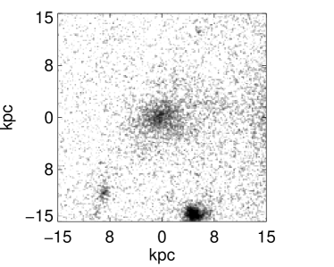
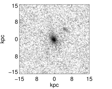
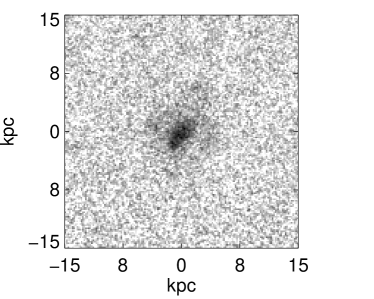
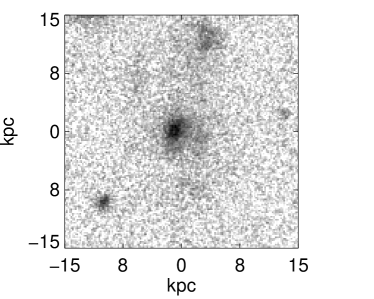
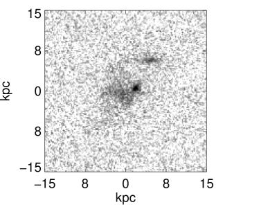
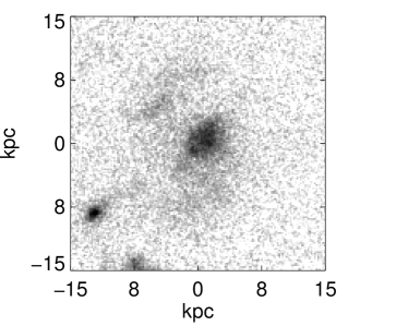
Figure 10: Images in $z$ band of the 8 distant giant LSB galaxies. For comparison, the last image at the bottom shows the simulated distant (GOODS) giant LSB.

The light profile of the 36 local and 36 distant simulated giant LSBs was then decomposed using GALFIT and analysed using the method described in Sect. 3.2. The mean and r.m.s. values of the differences between the initial and fitted values of the bulge and disc $r_{d}$ and $\mu_{0}$ were derived, as listed in Tab. 5. Fig. 11 shows the results corresponding to the case sampling the mean disc values projected into the local and distant samples.

Table 5: Mean$\pm$r.m.s. values of the differences between the initial and fitted parameters over the 36 simulated local and 36 simulated distant giant LSBs. All the parameters were let free during the fitting process.

Parameter	Mean (initial-fitted)	$\sigma$ (initial-fitted)
	SDSS	GOODS
Bulge
$\mu_{0}$ (mag/arcsec2)	0.14$\pm$0.02	0.33$\pm$0.02
$r_{d}$ (kpc)	-0.13$\pm$0.02	-0.11$\pm$0.03
$n$	-0.12$\pm$0.01	-0.18$\pm$0.02
Disc
$\mu_{0}$ (mag/arcsec2)	-0.07$\pm$0.04	-0.06$\pm$0.04
$r_{d}$ (kpc)	-0.58$\pm$0.15	-0.77$\pm$0.25

Tab. 5 shows that the extended LSB discs can be well recovered both in the local and distant samples. The only significant effects are a slight underestimation of the bulge central surface brightness (in particular for the distant sample), while it is accurately recovered for the giant LSB discs, and a trend for the giant LSB discs to be underestimated in size both in the local and distant samples. We conclude that the morphological decomposition described in Sect. 3.2 provide robust identifications of faint giant LSB discs, and that the lack of detection of giant LSBs in the local sample cannot be due to differences in surface brightness limits between the two surveys, as expected from App. A.

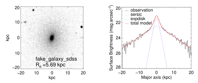
Figure 11: Simulated giant LSB images and light profiles for the SDSS (upper panel) and GOODS (lower panel) surveys. The right panels show the light profiles along the major axis over which the profile of the model that has been fitted has been superimposed.

Appendix C The SDSS $frac\_DeV$ parameter vs. the bulge-to-total light ratio.

The reduction pipeline of the SDSS database (Stoughton et al. 2002) produces an automatic fit of each galaxy profile. Their code fits two models in each band: a pure de Vaucouleurs profile truncated at $7r_{eff}$, and a pure exponential profile truncated at $3r_{eff}$. Their fit takes into account the PSF modelled by a double Gaussian. The choice of fitting only one component instead of a more complicated model is motivated by the huge amount of data and the computational expense of such a process. A linear combination of the best-fit de Vaucouleurs and exponential models is then re-fitted to the galaxy image. The fraction of the de Vaucouleurs profile in the resulting fit is recorded as the $frac\_deV$ parameter. In many papers this parameter is used to distinguish between early and late-type galaxies, or even as a proxy for the bulge-to-total light ratio (an elliptical galaxy is expected to have $frac\_deV>0.5$, while a pure disc galaxy is expected to have $frac\_deV<0.5$, see, e.g., Masters et al. 2010; Zhong et al. 2012 and references therein). We compare in Fig. 12 the B/T ratio derived from our full bulge/disc decomposition and the $frac\_deV$ parameter provided by the SDSS database in $r$ band. We find no clear correlation between the two parameters, although it can be noticed that the disc galaxies in the sample with B/T$<$0.1 all have $frac\_deV<0.4$, and that except for one object, all the elliptical galaxies have $frac\_deV>0.45$. The spiral galaxies in the sample with 0.2$<$B/T$<$0.5 all have $frac\_deV>0.8$, which means that they could be classified as S0 or E galaxies using this criterion only.

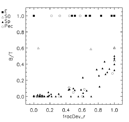
Figure 12: Comparison between the bulge-to-total light ratio and the SDSS $frac\_deV$ parameter for the local sub-sample of galaxies with $b/a>0.5$, in $r$ band.

References

- Abazajian et al. (2009) Abazajian K. N. et al., 2009, ApJS, 182, 543
- Barth (2007) Barth A. J., 2007, AJ, 133, 1085
- Bell et al. (2003) Bell E. F., McIntosh D. H., Katz N., Weinberg M. D., 2003, ApJS, 149, 289
- Bertin & Arnouts (1996) Bertin E., Arnouts S., 1996, A&AS, 117, 393
- Blanton et al. (2003) Blanton M. R. et al., 2003, ApJ, 592, 819
- Blanton et al. (2005) Blanton M. R., Lupton R. H., Schlegel D. J., Strauss M. A., Brinkmann J., Fukugita M., Loveday J., 2005, ApJ, 631, 208
- Boissier et al. (2008) Boissier S. et al., 2008, ApJ, 681, 244
- Charlot, Worthey & Bressan (1996) Charlot S., Worthey G., Bressan A., 1996, ApJ, 457, 625
- Contini et al. (2016) Contini T. et al., 2016, A&A, 591, A49
- Dahlen et al. (2010) Dahlen T. et al., 2010, ApJ, 724, 425