A Maximum A Posteriori Estimation Framework for Robust High Dynamic Range Video Synthesis

Abstract

High dynamic range (HDR) image synthesis from multiple low dynamic range (LDR) exposures continues to be actively researched. The extension to HDR video synthesis is a topic of significant current interest due to potential cost benefits. For HDR video, a stiff practical challenge presents itself in the form of accurate correspondence estimation of objects between video frames. In particular, loss of data resulting from poor exposures and varying intensity make conventional optical flow methods highly inaccurate. We avoid exact correspondence estimation by proposing a statistical approach via maximum a posterior (MAP) estimation, and under appropriate statistical assumptions and choice of priors and models, we reduce it to an optimization problem of solving for the foreground and background of the target frame. We obtain the background through rank minimization and estimate the foreground via a novel multiscale adaptive kernel regression technique, which implicitly captures local structure and temporal motion by solving an unconstrained optimization problem. Extensive experimental results on both real and synthetic datasets demonstrate that our algorithm is more capable of delivering high-quality HDR videos than current state-of-the-art methods, under both subjective and objective assessments. Furthermore, a thorough complexity analysis reveals that our algorithm achieves better complexity-performance trade-off than conventional methods.

I Introduction

High dynamic range (HDR) images, with several orders higher dynamic range than conventional low dynamic range (LDR) images, are capable of faithfully carrying full information of natural scenes [1]. This advantage has brought HDR imaging into a wide range of application areas, including game and movie industries [1]. However, digital imaging devices designed for directly capturing HDR images are generally prohibitively expensive to be employed in practical applications [2, 3, 4]. An alternative approach is to merge multiple images of the same scene taken with varying exposure times [5]. However, directly merging multiple LDR frames is prone to bringing in ghosting artifacts. Therefore, to address such an issue, a lot of ghost-free HDR imaging techniques have been proposed [6, 7, 8, 9]. For a comprehensive survey on this literature, we refer the readers to [10, 1].

(a)

(b)

​

Figure 1: A simple extension of the state-of-the-art HDR imaging algorithm [7] to HDR video synthesis fails to produce high-quality HDR frames. (a) The original LDR frame, (b) HDR frame synthesized by Hu et al.’s HDR imaging algorithm [7]. Video result available at https://youtu.be/K_MkSxMURXo.

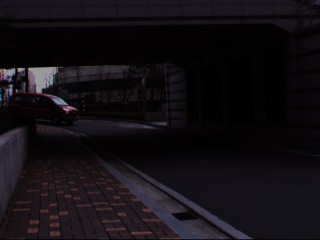
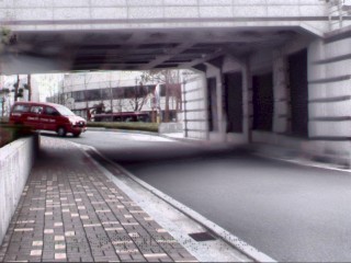
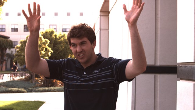
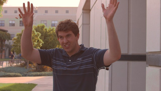
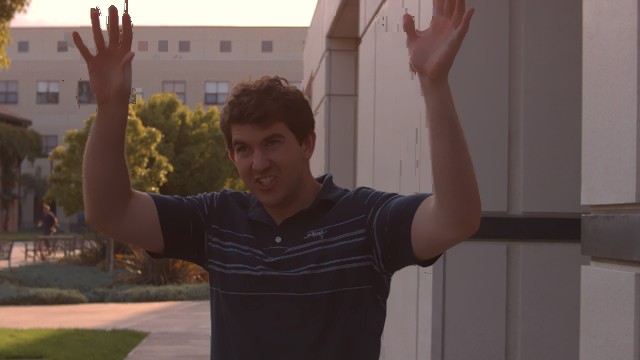
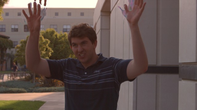
Similar to HDR image synthesis, HDR video synthesis has also become an active research topic, as there is a growing demand for HDR videos. The transition from HDR imaging to HDR video seems straightforward. Instead of capturing multiple images of the same scene with varying exposures, one can alternate the exposure times between successive frames, and then synthesize several consecutive frames together repeatedly on a frame basis to form an HDR video [11]. However, despite the popularity of HDR imaging, only a limited number of algorithms have been proposed to synthesize HDR videos through the aforementioned approach. Although we may apply the existing ghost-free HDR imaging techniques to HDR video synthesis through the sliding window approach, such a simple extension fails to provide high-quality HDR video frames. Fig. 1 shows such an example, in which the state-of-the-art ghost-free HDR imaging algorithm [7] suffers from visually objectionable artifacts. The major challenge in HDR video synthesis is to establish accurate correspondences between successive frames with different exposures. Specifically, the violation of the constant intensity assumption made typically by optical flow methods [12, 13] together with the presence of under-exposed or saturated regions imposes great challenges on the computation of optical flow. Moreover, since the input LDR video frames are typically taken with two to three different exposure times, unlike the case in HDR image synthesis where multiple exposure times are allowed, content loss due to under-exposure or saturation is even more severe. As a consequence, direct application of ghost-free HDR image synthesis techniques to HDR video usually yields poor results.

Due to the aforementioned challenges, a vast majority of research on HDR video focuses on hardware-based approaches [3, 4, 14]. However, these methods need specially designed devices and are typically prohibitively expensive. Therefore, software-based approaches via synthesis of alternatively exposed LDR frames still have their merits, as they only require conventional cameras. Recent work has focused on addressing HDR video synthesis challenges at an algorithmic level. In [11], Kang et al. compensated the exposure differences between frames by adjusting their exposures through the camera response function, and then applied conventional optical flow techniques to estimate correspondences. However, their method relies heavily on the accuracy of the optical flow estimation, and it usually fails when complex motions exist. To increase the robustness of optical flow, Mangiat and Gibson [15] developed a block-based motion estimation technique instead of the conventional gradient-based ones [12, 16]. They further alleviated registration errors by post-processing with a modified bilateral filter, called HDR filter [17], and applied it to large scale security and surveillance [18]. In [19], Kalantari et al. composed optical flow based registration with patch-based synthesis [6] to handle complex motions. In their method, temporal coherency is enhanced by optical flow, while incorrect correspondences are corrected by patch-based synthesis. Although their algorithm usually provides high-quality HDR video sequences, they may distort moving objects and introduce color artifacts.

Motivations and Contributions: The stiff challenge in HDR video synthesis is in the exact correspondence estimation between input frames taken with different exposures. To address the challenge, we avoid the correspondence estimation by formulating HDR video synthesis statistically as a MAP estimation problem, which subsequently reduces to an optimization problem that implicitly captures motion information. Specifically, each video frame is separated into a static background and a sparse foreground, which can be synthesized via rank minimization and multiscale adaptive kernel regression, respectively. Compared with conventional approaches, our algorithm for the first time introduces MAP estimation approach, as well as kernel regression method into the literature of HDR video synthesis. We call it MAP-HDR. Further, we improve kernel regression to make it locally adaptable in handling motion and dealing with missing (saturated/dark) samples by solving an unconstrained optimization problem. Our major contributions in this work are summarized as follows.

1. A novel MAP estimation framework: We develop, for the first time, a MAP estimation framework for HDR image and video synthesis. It can be shown that many existing techniques in [8, 9] can be regarded as specific instances of this framework. Furthermore, based on reasonable statistical assumptions and appropriate choice of statistical models, we can reduce the general MAP estimation framework towards a specific optimization problem, whose solution provides synthesized HDR video frames.

2. Multiscale adaptive kernel regression approach: We develop a novel multiscale adaptive kernel regression approach. In this work, we apply it to the synthesis of foreground radiance data, as part of our MAP-HDR algorithm. Its effectiveness in accurate HDR data estimation is demonstrated through extensive experiments.

3. Experimental validation and insight: We evaluate the merits of the MAP-HDR algorithm on both real-world and synthetic datasets. Experimental results demonstrate that our algorithm is capable of producing high-quality artifact-free HDR videos both under subjective and objective assessments, particularly in the face of complex motion when many state-of-the-art methods fail.

4. Complexity analysis: We carry out a thorough complexity analysis over the MAP-HDR algorithm as well as the state-of-the-art HDR video synthesis methods. Our algorithm turns out to be of comparable complexity with state-of-the-art methods, while providing higher-quality results. Thus, our algorithm achieves a better complexity-performance trade-off.

5. Reproducibility: All the datasets and the MATLAB code for producing the experimental results in this paper are publicly available online on our project website.

The rest of the paper is organized as follows: Section II provides a succinct review of various kernel regression techniques. Section III describes the general formulation of HDR video synthesis through MAP estimation and develops a novel multiscale adaptive kernel regression approach to estimate foreground data. Section IV discusses implementation details of the proposed MAP-HDR algorithm. Section V shows the effectiveness of the MAP-HDR algorithm by comparison against several state-of-the-art methods both subjectively and objectively, and a computational complexity analysis is provided. Finally, Section VI concludes this paper.

II Preliminaries of Kernel Regression

For the sake of completeness, we briefly review the classical kernel regression (CKR) and its variants in [21, 22], on which the proposed algorithm is based. CKR refers to the technique of minimum mean squared error (MMSE) estimation of regression function through local polynomial approximation. Suppose that we aim to estimate the regression relationship $z(\cdot)$ between a set of data samples $\{y_{i}\in\mathbb{R}\}_{i=1}^{P}$ and their locations $\{{\bf x}_{i}\in\mathbb{R}^{d}\}_{i=1}^{P}$, given by

$$y_{i}=z({\bf x}_{i})+\varepsilon_{i},\quad i=1,\dots,P.$$ (1)

Assuming that $z(\cdot)$ is smooth, by the Taylor’s formula, we can approximately expand it locally as a polynomial around some point ${\bf x}$ near the sample location ${\bf x}_{i}$, i.e.,

$$z({\bf x}_{i})\approx z({\bf x})+\nabla z^{T}({\bf x}_{i}-{\bf x})+\frac{1}{2}({\bf x}_{i}-{\bf x})^{T}\mathcal{H}(z)({\bf x}_{i}-{\bf x})+\cdots,$$ (2)

where $\nabla z$ and $\mathcal{H}(z)$ denote the gradient and Hessian of $z(\cdot)$ at ${\bf x}$, respectively. By parametrizing its polynomial expansion, the estimation of $z(\cdot)$ can be simplified as the following weighted linear least square problem:

$$\min_{\{\bm{\beta}_{k}\}}\;\sum_{i=1}^{P}[y_{i}-\beta_{0}-\bm{\beta}_{1}^{T}({\bf x}_{i}-{\bf x})-\cdots]^{2}K_{h}({\bf x}_{i}-{\bf x}),$$ (3)

where $K_{h}(\cdot)$ is the kernel function for imposing weights on each squared error term. Its parameter $h$ is called bandwidth, which controls the extent of smoothing. A commonly used kernel function is the Gaussian kernel, given by

$$K_{h}({\bf u})=\frac{1}{(2\pi)^{\frac{d}{2}}h^{d}}\exp\!\left(-\frac{\|{\bf u}\|^{2}}{2h^{2}}\right)\!.$$ (4)

In [21], Takeda et al. developed an iterative steering kernel regression (ISKR) scheme in 2D and showed that it can be successfully applied to various image processing applications, including denoising, interpolation, and super-resolution. Further, in [22], it was shown that state-of-the-art performance can be achieved in video super-resolution by generalizing ISKR to 3D, called 3D ISKR. The major advantage of ISKR over CKR is that the kernel function $K(\cdot)$ of ISKR is data-adaptive, i.e., it has the following form:

$$K_{{\bf H}_{i}}({\bf u})=\frac{\exp\!\left(-\frac{1}{2}{\bf u}^{T}{\bf H}_{i}^{-1}{\bf u}\right)}{(2\pi)^{\frac{d}{2}}\sqrt{\det({\bf H}_{i})}},$$ (5)

where ${\bf H}_{i}$ is called the steering matrix. At each sample location, the steering matrix is estimated from the structure tensor matrix [23] with some modifications on its singular values to avoid singularity and flatten its directionality, which would otherwise be too strong. By substituting $K_{h}(\cdot)$ in (3) with $K_{{\bf H}_{i}}(\cdot)$ and solving the weighted least square problem, we can obtain the optimal coefficients $\widehat{\bm{\beta}}$, given by

$$\widehat{\bm{\beta}}=({\bf X}^{T}{\bf K}{\bf X})^{-1}{\bf X}^{T}{\bf K}{\bf y},$$ (6)

where ${\bf y}=[y_{1},y_{2},\dots,y_{P}]^{T}$ is the data sample vector, and $\bm{{\bf K}}=\mathrm{diag}\{K_{{\bf H}_{i}}({\bf x}_{i}-{\bf x})\}_{i=1}^{P}$ is the diagonal weighting matrix with $K_{{\bf H}_{i}}({\bf x}_{i}-{\bf x})$ on the diagonal. For video processing, the data samples are collected from a local spatial-temporal 3D block, and typically the center of the block is the target pixel to be estimated. Also, ${\bf X}$, called design matrix, is given by

$${\bf X}=\begin{bmatrix}1&({\bf x}_{1}-{\bf x})^{T}&\mathrm{vech}^{T}\{({\bf x}_{1}-{\bf x})({\bf x}_{1}-{\bf x})^{T}\}&\dots\\ 1&({\bf x}_{2}-{\bf x})^{T}&\mathrm{vech}^{T}\{({\bf x}_{2}-{\bf x})({\bf x}_{2}-{\bf x})^{T}\}&\dots\\ \vdots&\vdots&\vdots&\vdots\\ 1&({\bf x}_{P}-{\bf x})^{T}&\mathrm{vech}^{T}\{({\bf x}_{P}-{\bf x})({\bf x}_{P}-{\bf x})^{T}\}&\dots\end{bmatrix},$$ (7)

where $\rm vech(\cdot)$ denotes the half-vectorization operator of the lower-triangular portion of a symmetric matrix [21].

III Proposed Algorithm (MAP-HDR)

III-A Image Acquisition Model

We first present an image acquisition model, on which the MAP-HDR algorithm is based. The charge collected by a sensor equals the product of the irradiance value $a$ and the exposure time $\Delta t$. Then, the resulting exposure value ($a\Delta t$) is corrupted by Gaussian random noise $n$. Finally, the pixel intensity value $z$ is obtained by the camera response function $g(\cdot)$ [5], a nonlinear mapping from the exposure value to the pixel intensity value. Fig. 2 depicts this physical process; more formally, this process can be expressed by

$$z=g(a\Delta t+n).$$ (8)

For a well-exposed pixel, the camera response function is invertible at its radiance level. Then, the conditional probability density of $z$ given the knowledge of $a$ is given by

$$f(z|a) =\frac{d}{dz}\mathrm{Pr}\{g(a\Delta t+n)<z\}$$

$$=\frac{d}{dz}\mathrm{Pr}\{a\Delta t+n<g^{-1}(z)\}$$

$$=\frac{d}{dz}\Phi\!\left(\frac{g^{-1}(z)-a\Delta t}{\sigma_{n}}\right)\!\propto\exp\!\left(-\frac{(a-\widehat{a})^{2}}{2\sigma_{n}^{2}/\Delta t^{2}}\right)\!,$$ (9)

where $\sigma_{n}$ and $\Phi$ denote the standard deviation of $n$ and the cumulative distribution function (CDF) of the standard Gaussian distribution, respectively, and $\widehat{a}=g^{-1}(z)/\Delta t$ is the estimated irradiance value.

Figure 2: Physical model for HDR image acquisition.

Suppose we are given $N$ consecutive frames, taken with alternating exposures, i.e., long and short. Each frame consists of $K$ pixels. We separate each frame into foreground and background regions. To this end, we first define a binary matrix ${\bf S}\in\{0,1\}^{K\times N}$ that supports foreground regions as

$$S_{ij}=\begin{cases}1,&\text{if pixel $(i,j)$ is in foreground},\\ 0,&\text{if pixel $(i,j)$ is in background}.\end{cases}$$ (10)

Then, we develop a probabilistic model of ${\bf S}$ based on the assumption that the interactions of a given pixel with all the others are wholly described by its neighbors, i.e., it satisfies the Markov property. Then, we model ${\bf S}$ as a Markov random field (MRF) to exploit the spatial interactive relationship among pixels. In this work, we employ the Ising model [24], which is known to be simple yet effective in modeling interactions between neighboring pixels [25]. Specifically, the probability density function (PDF), which can be regarded as the prior probability of ${\bf S}$, is given by

$$f({\bf S})\propto\exp\!\left(-\sum_{(i,j)\in{\mathcal{E}}}w_{ij}s_{i}s_{j}-\sum_{i\in{\mathcal{V}}}\lambda_{i}s_{i}\right)\!,$$ (11)

where $\mathcal{V}$ and $\mathcal{E}$ denote the sets of vertices and edges of the graphical representation of ${\bf S}$, respectively, and $w_{ij}$ and $\lambda_{i}$ are the edge interaction costs and vertex weights. Also, $s_{i}\in\{0,1\}$ corresponds to the $i$-th pixel in ${\bf S}$.

III-B MAP Estimation-based HDR Video Synthesis

We make two assumptions on the input videos. First, scene information is included in either of alternating (exposure) frames. Second, global camera motions as well as local object motions between adjacent frames are bounded, i.e., they can be reasonably but not arbitrarily large.

Based on these assumptions, we formulate HDR video synthesis as a MAP estimation problem based on the probabilistic model in (11). Let ${\bf D}:=[{\mathrm{vec}}(I_{1}),{\mathrm{vec}}(I_{2}),\dots,{\mathrm{vec}}(I_{N})]$ denote the observation matrix of a scene, where each $I_{k}$ is the observed irradiance map of the $k$-th frame obtained by the camera response function [5]. As mentioned earlier, we separate each frame into foreground and background regions to consider object motions between input frames. Let ${\bf F}$ and ${\bf B}$ denote matrices of the inherent foreground and background irradiance, respectively. Then, the irradiance matrix ${\bf A}$ for the synthesized HDR video can be obtained by

$${\bf A}={\mathcal{P}}_{{\bf S}}({\bf F})+{\mathcal{P}}_{{\bf S}^{\mathsf{c}}}({\bf B}),$$ (12)

where ${\mathcal{P}}_{\bf S}({\bf Y})$ denotes the sampling operator defined by

$$\left[{\mathcal{P}}_{\bf S}({\bf Y})\right]_{ij}=\begin{cases}Y_{ij},&\mbox{if $S_{ij}=1$},\\ 0,&\mbox{otherwise}.\\ \end{cases}$$

Note, however, that the foreground and background regions ${\bf F}$ and ${\bf B}$, respectively, and the foreground support ${\bf S}$ are unknown in (12). Therefore, we estimate ${\bf B}$, ${\bf F}$, and ${\bf S}$ given the observation ${\bf D}$. Specifically, let $f({\bf S},{\bf B},{\bf F}|{\bf D})$ denote the joint probability of ${\bf S}$, ${\bf B}$, and ${\bf F}$ given ${\bf D}$. Then, we formulate the estimation of ${\bf S}$, ${\bf B}$, and ${\bf F}$ as the following MAP estimation problem:

$$(\widehat{{\bf S}},\widehat{{\bf B}},\widehat{{\bf F}})=\underset{{\bf S},{\bf B},{\bf F}}{\arg\max}\;f({\bf S},{\bf B},{\bf F}|{\bf D}).$$ (13)

For simplicity, we assume Lambertian surfaces, where all irradiance maps are normalized by subtracting its minimum value and dividing by its range. Then, we can make following two independence assumptions. First, the irradiance values depend only on the properties of the objects, and thus the irradiance values of the foreground objects and the background scenes are statistically independent, i.e.,

$$f({\mathcal{P}}_{{\bf S}^{\mathsf{c}}}({\bf Y}),{\mathcal{P}}_{\bf S}({\bf Y}))=f({\mathcal{P}}_{{\bf S}^{\mathsf{c}}}({\bf Y}))f({\mathcal{P}}_{\bf S}({\bf Y})),$$ (14)

where ${\bf Y}={\bf D},{\bf A}$. Second, we assume that the irradiance at each pixel is independent of ${\bf S}$, provided that we know whether it belongs to foreground or background. In other words,

$$f({\mathcal{P}}_{\bf S}({\bf Y})|{\bf S}) =f({\mathcal{P}}_{\bf S}({\bf Y})),$$ (15)

$$f({\mathcal{P}}_{{\bf S}^{\mathsf{c}}}({\bf Y})|{\bf S}) =f({\mathcal{P}}_{{\bf S}^{\mathsf{c}}}({\bf Y})).$$ (16)

Then, based on the statistical assumptions in (14)–(16), we can rewrite the estimation problem in (13) as

$$(\widehat{{\bf S}},\widehat{{\bf B}},\widehat{{\bf F}})=\underset{{\bf S},{\bf B},{\bf F}}{\arg\max}\;\log f({\mathcal{P}}_{{\bf S}^{\mathsf{c}}}({\bf D})|{\bf B})+\log f({\bf B})$$

$$+\log f({\mathcal{P}}_{\bf S}({\bf F})|{\mathcal{P}}_{\bf S}({\bf D}))+\log f({\mathcal{P}}_{{\bf S}}({\bf D}))+\log f({\bf S}).$$ (17)

The detailed derivation of (17) is provided in Appendix A.

First, recall that ${\bf D}$ is the observation of ${\bf A}$ with noise. Thus, from the observation model in (9) with the Gaussian noise, we can approximate the first term in (17) $\log f({\mathcal{P}}_{{\bf S}^{\mathsf{c}}}({\bf D})|{\bf B})$ as negatively proportional to $\|{\mathcal{P}}_{\Omega}({\bf D}-{\bf B})\|_{F}^{2}$, where $\Omega$ denotes the support of well-exposed background, given by $\Omega:={\mathcal{P}}_{{\bf S}^{\mathsf{c}}}({\bf M})$, and $\|{\bf Y}\|_{F}:=\big{(}\sum_{ij}|Y_{ij}|^{2}\big{)}^{1/2}$ is the Frobenius norm of a matrix. Here, $M_{ij}=1$ if a pixel intensity $Z_{ij}$ satisfies $Z_{\rm th}<Z_{ij}<Z_{\max}-Z_{\rm th}$, where $Z_{\rm th}$ and $Z_{\max}$ are the threshold value and maximum pixel intensity, respectively, and $M_{ij}=0$ otherwise. Note that we use $\Omega$ instead of ${\bf S}^{\mathsf{c}}$. This is based on the observation that the derivations in (9) holds only for well-exposed pixels and ill-exposed pixels are invalid, since they are constant independent of ${\bf B}$.

Second, considering that the background scene is static, we regard $f({\bf B})$ as a low-rank prior of the background scene matrix. More specifically, $f({\bf B})=\frac{1}{C}\exp(-\alpha\|{\bf B}\|_{\ast})$ with a normalization constant $C$, where $\|{\bf B}\|_{*}=\sum_{k}\sigma_{k}({\bf B})$ denotes the nuclear norm, and $\sigma_{k}({\bf B})$ is the $k$-th largest singular value of ${\bf B}$. Note that the low-rank prior plays a role similar to the Laplacian prior in the structured sparsity model [26]. In addition, as discussed in Section III-A, the last term $\log f({\bf S})$ in (17) is given by (11).

Third, we choose a conditional Gaussian distribution for ${\mathcal{P}}_{\bf S}({\bf F})|{\mathcal{P}}_{\bf S}({\bf D})$, then $\log f({\mathcal{P}}_{\bf S}({\bf F})|{\mathcal{P}}_{\bf S}({\bf D}))\propto-\|{\bf C}^{-\frac{1}{2}}{\mathcal{P}}_{\bf S}({\bf F}-{\bf E})\|_{F}^{2}$, where ${\bf E}=\mathcal{E}[{\mathcal{P}}_{\bf S}({\bf F})|{\mathcal{P}}_{\bf S}({\bf D})]$, ${\bf C}$ is the covariance matrix of ${\mathcal{P}}_{\bf S}({\bf F})|{\mathcal{P}}_{\bf S}({\bf D})$. Note that ${\bf E}$ corresponds to the MMSE estimator of ${\bf F}$ given ${\bf D}$. Also, we choose a Laplacian prior for $f({\mathcal{P}}_{\bf S}({\bf D}))$, i.e., $\log f({\mathcal{P}}_{\bf S}({\bf D}))\propto-\|{\mathcal{P}}_{\bf S}({\bf D})\|_{1}=-\sum_{i}d_{i}s_{i}$, where $d_{i}$ and $s_{i}$ are the elements of ${\bf D}$ and ${\bf S}$, respectively. Note that, since $s_{i}$ is binary, an improper choice of the prior would result in an intractable combinatorial optimization problem [27].

Then, under these simplifications, we reformulate the MAP estimation in (17) as the following optimization problem:

$$(\widehat{{\bf S}},\widehat{{\bf B}},\widehat{{\bf F}}) =\underset{{\bf S},{\bf B},{\bf F}}{\arg\min}\;\frac{1}{2}\|{\mathcal{P}}_{\Omega}({\bf D}-{\bf B})\|_{F}^{2}+\alpha\|{\bf B}\|_{\ast}+\beta\|{\bf S}\|_{1}$$

$$\quad+\gamma\|{\bf W}{\mathrm{vec}}({\bf S})\|_{1}+\|{\bf C}^{-\frac{1}{2}}{\mathrm{vec}}({\mathcal{P}}_{\bf S}({\bf F}-{\bf E}))\|^{2}_{F},$$ (18)

where ${\bf W}$ is the weighting matrix that accounts for the interactions between neighboring pixels, and $\alpha,\beta,\gamma>0$ are constant parameters to control the relative importance between each term.

Notice that, in (18), for any fixed ${\bf S}$, we can obtain ${\mathcal{P}}_{\bf S}(\widehat{{\bf F}})={\mathcal{P}}_{\bf S}(\widehat{{\bf E}})$. Thus, ${\bf F}$ can be considered independent of other terms, and we can separate the optimization in (18) into two subproblems, i.e.,

$$(\widehat{{\bf S}},\widehat{{\bf B}}) =\underset{{\bf S},{\bf B}}{\arg\min}\;\frac{1}{2}\|{\mathcal{P}}_{\Omega}({\bf D}-{\bf B})\|_{F}^{2}+\alpha\|{\bf B}\|_{\ast}$$

$${}\qquad+\beta\|{\bf S}\|_{1}+\gamma\|{\bf W}{\mathrm{vec}}({\bf S})\|_{1}$$ (19)

and

$${\mathcal{P}}_{\widehat{{\bf S}}}(\widehat{{\bf F}})=\mathcal{E}\!\left[{\mathcal{P}}_{\widehat{{\bf S}}}({\bf F})|{\mathcal{P}}_{\widehat{{\bf S}}}({\bf D})\right]\!.$$ (20)

A solution to the subproblem in (19) can be obtained by the rank minimization for HDR deghosting [8]. Then, it remains to find $\mathcal{E}\!\left[{\mathcal{P}}_{\widehat{{\bf S}}}({\bf F})|{\mathcal{P}}_{\widehat{{\bf S}}}({\bf D})\right]$. In this work, we propose to employ kernel regression [21], which is a widely-used MMSE approach. In [22], kernel regression has been proven to be effective in implicitly capturing motion information and interpolating missing pixels, thus rendering high-quality video results. Let us now describe how to extend the standard kernel regression [21] to deal with HDR data.

III-C Locally Adaptive Kernel Regression via Optimization

Since HDR video synthesis can be regarded as a video reconstruction problem, i.e., recovery of data in saturated or under-exposed regions, kernel regression is a natural choice to be considered. However, direct application of kernel regression techniques, including the classical ones and their variants, to HDR video synthesis may fail to generate high-quality videos, for the following reasons:

1. HDR data are usually noisy and grainy after exposure adjustment, which degrades the performance of kernel regression. Specifically, reliable estimation of the steering matrices in such regions is generally difficult.

2. Some regions in HDR frames may be missing due to saturation or under-exposure. The polynomial approximation of kernel regression may fail to represent underlying data faithfully in such regions, especially where a significant portion of pixels are missing.

3. HDR data varies significantly in intensity values, and even after exposure adjustment the intensity differences between frames may still be significant, making the data in different frames biased.

(a) Short exposure

(b) Long exposure

Figure 3: Plots of weighting function $\phi_{i}$.

We develop a locally adaptive kernel regression method to address the aforementioned issues for HDR video synthesis. Firstly, to address 1), we impose a radiometric weight $\nu_{i}$ for pixel $i$, defined by $\nu_{i}=\phi_{i}\omega_{i}$, where $\phi_{i}$ assigns lower weights to less properly exposed pixels as depicted in Fig. 3. For the center pixel index $c$ to be estimated, $\omega_{i}$ is defined as

$$\omega_{i}=\begin{cases}e^{-\sigma(y_{i}-y_{c})_{+}^{2}},&\text{if reference frame is long exposure,}\\ e^{-\sigma(y_{c}-y_{i})_{+}^{2}},&\text{otherwise,}\end{cases}$$ (21)

with $\sigma=\kappa(1-w_{c})$ for some positive constant $\kappa$ and $x_{+}:=\max\{x,0\}$. When the center pixel is saturated, $\omega_{i}$ encourages fitting towards higher values, but towards lower values when the center pixel is under-exposed.

Then, we reformulate the weighted least square problem in (3) as

$$\min_{\bm{\beta}}\;\;({\bf y}-{\bf X}\bm{\beta})^{T}\bm{\Lambda}({\bf y}-{\bf X}\bm{\beta})+\varepsilon\|\bm{\beta}\|_{2}^{2},$$ (22)

where ${\bf y}$ is the data sample vector, and $\bm{\Lambda}=\mathrm{diag}\{K_{{\bf H}}({\bf x}_{i}-{\bf x})\nu_{i}\}_{i=1}^{P}$ is the weighting matrix. Note that the Tikhonov regularization term $\|\bm{\beta}\|_{2}^{2}$ is added in (22) to prevent overfitting, and $\varepsilon>0$ is the regularization parameter to control its effect. Then, the optimal coefficients can be obtained as a closed-form solution to (22), given by

$$\widehat{\bm{\beta}}=({\bf X}^{T}\bm{\Lambda}{\bf X}+\varepsilon{\bf I})^{-1}{\bf X}^{T}\bm{\Lambda}{\bf y}.$$ (23)

In addition, we note that the computation of the structure tensor matrix is intractable in practice. Therefore, instead of explicitly computing the structure tensor matrix and using it to obtain the steering matrix, we determine it implicitly by minimizing the estimation error. More specifically, we try to find ${\bf H}$ that minimizes the weighted least squares error

$$({\bf y}-{\bf X}\widehat{\bm{\beta}})^{T}\bm{\Lambda}({\bf y}-{\bf X}\widehat{\bm{\beta}})+\varepsilon\|\widehat{\bm{\beta}}\|_{2}^{2}.$$ (24)

Since the covariance matrix must be symmetric positive definite (SPD), if we directly solve for it, a SPD constraint has to be imposed that is hard to deal with. Thus, we represent the inverse of steering matrix using its Cholesky factorization instead, given by

$${\bf H}={\bf R}^{\ast}{\bf R},$$ (25)

where ${\bf R}\in\mathbb{R}^{3\times 3}$ is some upper triangular matrix. In addition to removing the SPD constraint, using this representation can also bring down the dimensionality of the problem since ${\bf R}$ is upper triangular. However, simply minimizing (24) may cause overfitting. In particular, ${\bf R}$ may tends to either $0$ or infinity. In the former case, the kernel would be highly spread out, making the estimate undesirably blurred, while in the latter case, the obtained Gaussian kernel would be highly concentrated around ${\bf x}$, making the estimate strongly biased towards $z({\bf x})$. To prevent the former case, we use the unnormalized Gaussian kernel $\exp\left(-\frac{1}{2}\|{\bf R}{\bf u}\|_{2}^{2}\right)$. To avoid the latter case, i.e., to prevent ${\bf R}$ tending infinity, we propose to add the regularization term $\|{\bf R}\|_{F}^{2}$. In addition, since $\|{\bf R}\|_{F}^{2}=\mathrm{tr}({\bf R}^{*}{\bf R})=\|{\bf H}\|_{\ast}^{2}$, minimizing it jointly with (24) would effectively elongate and rotate the covariance matrix ${\bf H}$ along the local edge directions. As mentioned in Section II, this is the major characteristics of the steering matrix, the one we aim to estimate.

Secondly, we address 2) by modifying the polynomial fitting model in (3) as

$$y_{i}=\begin{cases}\beta_{0}+\bm{\beta}_{1}^{T}({\bf x}_{i}-{\bf x})+\dots,&\text{if pixel $i$ is well-exposed,}\\ t,&\text{otherwise,}\end{cases}$$ (26)

where $t=Z_{\mathrm{th}}$ when the reference frame is of lower exposure, and $t=Z_{\mathrm{max}}-Z_{\mathrm{th}}$ otherwise. Accordingly, the following cost term is added to (22)

$$\sum_{i=1}^{P}(1-\nu_{i})K_{\bf H}({\bf x}_{i}-{\bf x})(y_{i}-t)^{2}.$$ (27)

The cost term in (27) discourages ${\bf H}$ from steering towards dark pixels when the center pixel is saturated and toward bright pixels when the center pixel is under-exposed.

Finally, to address 3), we apply kernel regression to boosted [11] and Gamma-adjusted pixel values that are of less variations than the irradiance values. We extrapolate it when applying the camera response function to avoid data truncation.

Combining all the terms, we can formulate the estimation of the steering matrix as the following optimization problem:

$$\min_{{\bf R}}\;\; ({\bf y}-{\bf X}\widehat{\bm{\beta}}_{\bf R})^{T}\bm{\Lambda}_{\bf R}({\bf y}-{\bf X}\widehat{\bm{\beta}}_{\bf R})$$

$${}\;\;+({\bf y}-t{\bf 1})^{T}\widetilde{\bm{\Lambda}}_{{\bf R}}({\bf y}-t{\bf 1})+\varepsilon\|\widehat{\bm{\beta}}_{\bf R}\|_{2}^{2}+\lambda\|{\bf R}\|_{F}^{2},$$ (28)

where $\widetilde{\bm{\Lambda}}_{{\bf R}}:=\mathrm{diag}\{K_{\bf H}({\bf x}_{i}-{\bf x})(1-\nu_{i})\}$, $\varepsilon$ and $\lambda$ are positive regularization parameters, and ${\bf 1}\in\mathbb{R}^{P}$ is the vector containing all ones. Here, we explicitly put the subscript ${\bf R}$ to indicate the dependence on ${\bf R}$, i.e., $\bm{\Lambda}$, $\widetilde{\bm{\Lambda}}$, ${\bf K}$, and $\widehat{\bm{\beta}}$ are functions of ${\bf R}$. As $\varepsilon$ or $\lambda$ gets increased, the data becomes more smooth in general, as they play a role similar to that of bandwidth selection in CKR. However, the performance of our algorithm is less sensitive to the choice of $\varepsilon$ and $\lambda$ compared with the sensitivity of bandwith selection in CKR.

IV Implementation

IV-A Performance and Speed Improvements

Note that the cost function in (28) is smooth but nonconvex. Therefore, to solve the optimization, we employ the Broyden-Fletcher-Goldfarb-Shanno (BFGS) algorithm [28, 29, 30, 31], which is well-known for its fast convergence rate and robustness. In addition, we determine the gradient of (28) analytically via matrix calculus techniques, instead of approximating it numerically through finite differences. This can greatly speedup the optimization process, since significantly fewer matrix multiplications and inversions are required. Specifically, let $\mathcal{C}$ denote the cost function in (28), then, in Appendix B, we derive its gradient, which is given by

$$\nabla\mathcal{C} =\mathcal{UT}\Bigg{\{}2{\bf R}\sum_{i,j}k_{j}z_{j}({\bf x}_{j}-{\bf x})({\bf x}_{j}-{\bf x})^{T}$$

$$\qquad{}\times\left(k_{i}z_{i}J_{ij}-\lambda\widehat{\beta}_{i}T_{ij}\right)+2\mu{\bf R}$$

$$\quad{}-{\bf R}\!\sum_{i}\left(k_{i}z_{i}^{2}+\tilde{k}_{i}\tilde{z}_{i}^{2}\right)({\bf x}_{i}-{\bf x})({\bf x}_{i}-{\bf x})^{T}\Bigg{\}},$$ (29)

where ${\bf T}:=({\bf X}^{T}\bm{\Lambda}{\bf X}+\varepsilon{\bf I})^{-1}{\bf X}^{T}$, ${\bf J}:={\bf X}{\bf T}$, $k_{i}=\Lambda_{ii}$, $\tilde{k}_{i}=\widetilde{\Lambda}_{ii}$, $z_{i}:=y_{i}-\hat{y}_{i}$, $\tilde{z}_{i}:=y_{i}-t$, and $\widehat{y}_{i}$ are estimates of $y_{i}$ obtained by solving (22). Also, $\mathcal{UT}\{\cdot\}$ denotes the operator to extract the upper triangular part of a matrix.

In [22], second order polynomial model is employed both in spatial and temporal axes, and five to seven consecutive frames were shown to be helpful in preserving the details. However, in HDR video synthesis, usually only two to three frames are available. In this scenario, a second order polynomial has high risk of introducing large oscillations, producing visually noticeable artifacts. Therefore, we limit the order of polynomial to one (linear) in our implementation.

IV-B Pyramidal Framework for Handling Large Motions

Figure 4: The flowchart of multiscale kernel regression. We demonstrate its intermediate steps using one sample taken from the ParkingLot dataset. [32]

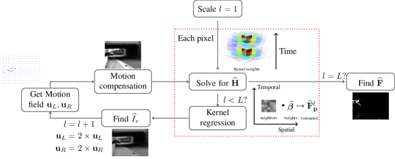
As kernel regression is performed on a small local block, it may fail to find correct correspondences for large motion, degrading the synthesis performance by introducing ghosting artifacts. To address such a limitation, we propose a pyramidal implementation of the aforementioned kernel regression method. Specifically, we first build an $L$-level Gaussian pyramid of the input frame, indexed from coarse to fine. At the $l$-th level, we first obtain an estimation of the reference frame. We apply the proposed locally adaptive kernel regression algorithm to obtain the foreground part, while filling in the background part with the scaled down version of the background matrix $\widehat{{\bf B}}$, obtained by solving (19). Then, we compute the motion fields among the estimated reference frame and its original neighboring frames using optical flow [13, 33, 34]. After the estimation process, exposure differences can be effectively alleviated, and hence motion estimation becomes reliable. We then scale up to the $(l+1)$th level and warp the neighboring frames towards the reference one using the previously obtained motion fields. On the finest level, we synthesize the warped irradiance frames using the aforementioned technique. Finally, to lower down the number of iterations in solving (28), we initialize all ${\bf H}$’s at the top level with identity matrices, which corresponds to CKR, and ${\bf H}$’s in $(l+1)$th level with those propagated from $l$th level. This strategy usually brings the initial ${\bf H}$’s closer to the optimal points, providing faster convergence. The overall flowchart of the proposed pyramidal implementation is depicted in Fig. 4

Algorithm 1 MAP-HDR Algorithm

0:  $I_{r-1}$, $I_{r}$, $I_{r+1}$, ${\bf M}$, $\alpha$, $\beta$, $\gamma$, $\kappa$, $\lambda$, $\mu$, $L$

1:  Initialize ${\bf S}_{1}\leftarrow{\bf M}$, ${\bf D}\leftarrow[{\mathrm{vec}}(I_{r-1}),{\mathrm{vec}}(I_{r}),{\mathrm{vec}}(I_{r+1})]$, ${\bf u}_{L}\leftarrow\mathbf{0}$, ${\bf u}_{R}\leftarrow\mathbf{0}$, and $k=1$.

2:  while stopping criteria not met do

3:     $\Omega\leftarrow{\mathcal{P}}_{{\bf S}_{k}^{\mathsf{c}}}({\bf M})$.

4:     ${\bf B}_{k+1}\leftarrow\underset{{\bf B}}{\arg\min}\;\frac{1}{2}\|\mathcal{P}_{\Omega}({\bf D}-{\bf B})\|_{F}^{2}+\alpha\|{\bf B}\|_{*}$.

5:     ${\bf S}_{k+1}\leftarrow\underset{{\bf S}\in\{0,1\}^{K\times N}}{\arg\min}\;\frac{1}{2}\|\mathcal{P}_{\Omega}({\bf D}-{\bf B}_{k+1})\|_{F}^{2}+\beta\|{\bf S}\|_{1}\newline \mbox{\hskip 35.56593pt}+\gamma\|{\bf W}{\rm vec}({\bf S})\|_{1}$.

6:     $k\leftarrow k+1$.

7:  end while

8:  $\widehat{{\bf B}}\leftarrow{\bf B}_{k}$, $\widehat{{\bf S}}\leftarrow{\bf S}_{k}$.

9:  $\{\widehat{{\bf B}}^{l}\}_{l=1}^{L}\leftarrow\mathrm{Pyr}(\widehat{{\bf B}})$, $\{\widehat{{\bf S}}^{l}\}_{l=1}^{L}\leftarrow\mathrm{Pyr}(\widehat{{\bf S}})$,
$\{{\bf D}^{l}\}_{l=1}^{L}\leftarrow\mathrm{Pyr}({\bf D})$, $\{{\bf M}^{l}\}_{l=1}^{L}\leftarrow\mathrm{Pyr}({\bf M})$.

10:  for $l=1$ to $L$ do

11:     ${\bf u}_{L}\leftarrow 2\times{\bf u}_{L}$, ${\bf u}_{R}\leftarrow 2\times{\bf u}_{R}$.

12:     $\widehat{I}_{r-1}^{l}\leftarrow\mathcal{W}_{{\bf u}_{L}}(I_{r-1}^{l})$, $\widehat{I}_{r+1}^{l}\leftarrow\mathcal{W}_{{\bf u}_{R}}(I_{r+1}^{l})$.

13:     for all ${\bf p}\in\mathrm{Supp}\{{\bf S}^{l}\}$ do

14:        Find $\widehat{{\bf H}}$ by solving (28).

15:        Find $\widehat{\bm{\beta}}$ from (23).

16:        $\widehat{{\bf F}}^{l}_{\bf p}\leftarrow{\bf e}_{1}^{T}\widehat{\bm{\beta}}$.

17:     end for

18:     $\widehat{I}^{l}_{r}\leftarrow{\mathcal{P}}_{{\bf S}^{l}}(\widehat{{\bf F}}^{l})+{\mathcal{P}}_{{({\bf S}^{l}})^{\mathsf{c}}}(\widehat{{\bf B}}^{l})$.

19:     if $l\neq L$ then

20:        ${\bf v}_{L}\leftarrow\mathrm{ME}(\widehat{I}^{l}_{r},\widehat{I}^{l}_{r-1})$, ${\bf v}_{R}\leftarrow\mathrm{ME}(\widehat{I}^{l}_{r},\widehat{I}^{l}_{r+1})$.

21:        ${\bf u}_{L}\leftarrow{\bf u}_{L}+{\bf v}_{L}$, ${\bf u}_{R}\leftarrow{\bf u}_{R}+{\bf v}_{R}$.

22:     end if

23:  end for

23:  $\widehat{I}_{r}$

Putting all the pieces together, our HDR video synthesis algorithm for synthesizing one HDR frame can be summarized in Algorithm 1. We use $\mathrm{Pyr}({\bf X})$ to denote the pyramidal decomposition of ${\bf X}$ and ${\bf X}_{{\bf p}}$ to denote one pixel of image ${\bf X}$ at location ${\bf p}$, ${\bf X}^{l}$ to denote the scaled-down version of ${\bf X}$ in the $l$-th level, and $\mathrm{ME}(I_{1},I_{2})$ to denote motion estimation between frame $I_{1}$ and $I_{2}$. Also, $r$ is the reference index, $I_{r}$, $I_{r-1}$, and $I_{r+1}$ denote the reference frame, its previous and next frames, respectively, and $\mathcal{W}_{\bf u}(I)$ denotes the warping operator on $I$ using motion field ${\bf u}$.

V Experiments and Discussions

TABLE I: Exposure times in seconds for each dataset.

	Students	Hallway2	ParkingLot	Bridge2
Long	0.005	0.005	0.012	5
Short	0.0005	0.0005	0.001	0.25

We evaluate the performance of the proposed MAP-HDR algorithm on seven challenging test video sequences shown in Figs. 5–10: Fire [19], Bridge2 [4], ParkingLot [32], Hallway2 [4], Students [4], ThrowingTowel [19], and WavingHands [19]. These test videos cover various scenarios, including large camera and/or object motions, significant over- and/or under-exposures. For the Fire, ThrowingTowel and WavingHands datasets, the alternating frames are available, while ground-truth radiance data for all the others exists. We therefore generate the alternating frames of those sequences from the original data by simulating the image acquisition procedure, i.e., by alternating the exposure times using the camera response function to obtain LDR frames. Specifically, we use the camera response function from [19], and set exposure times so that the majority of the scenes are properly exposed in either the short or long exposure. The exposure times for each video are listed in Table I. In all experiments, $\alpha$ in (18), $\epsilon$ and $\lambda$ in (28), and $\varepsilon$ in (23) are fixed to $0.5$, $0.01$, and $0.1$, respectively. The parameters $\beta$ and $\gamma$ in (18) are set online at each iteration, i.e., automatically updated at each iteration. Specifically, $\beta$ is set to $0.5\hat{\sigma}^{2}$, where $\hat{\sigma}$ is the standard deviation of elements in ${\mathcal{P}}_{{\bf S}_{k}^{\mathsf{c}}}({\bf D}-{\bf B}_{k})$, and $\gamma=\beta$. For Students, however, as the intensity variations are small, we set $\beta$ to be $0.01\hat{\sigma}^{2}$ and $\gamma=0.005\beta$. We vary pyramidal level $L$ from $2$ to $4$ according to the magnitudes of object motions to ensure a good compromise between computational cost and accuracy in correspondences. We define the weighting matrix ${\bf W}$ in (18) as

$$W_{i,j}=\begin{cases}w_{s},&\text{if pixel $(i,j)$ is a spatial neighbor, }\\ w_{t},&\text{if pixel $(i,j)$ is a temporal neighbor, }\\ 0,&\text{otherwise. }\end{cases}$$ (30)

We set $w_{s}=0.2$ and $w_{t}=40$ for Students dataset, while $w_{s}=20$ and $w_{t}=20$ for all the others. We experimentally found that MAP-HDR is robust to the choice of parameters in terms of performance.

We compare the performance of the MAP-HDR algorithm with three state-of-the-art HDR video synthesis methods: Kang et al.’s algorithm [11], Mangiat and Gibson’s algorithm [15, 17], and Kalantari et al.’s algorithm [19]. For Kang et al.’s algorithm, we used our own implementation, while for Mangiat and Gibson’s and Kalantari et al.’s, we executed the codes provided by the authors [35, 36] with the optimal parameter settings to provide the best overall visual quality. To print the synthesized HDR frames, we use the photographic tonemapping technique [37] in all the experiments with the same parameter settings as in [19].

V-A Subjective Video Quality Assessment

Input

(a)

(b)

(c)

(d)

(e)

​  ​  ​  ​

Kang

(f)

(g)

(h)

(i)

(j)

​  ​  ​  ​

Mangiat

(k)

(l)

(m)

(n)

(o)

​  ​  ​  ​

Kalantari

(p)

(q)

(r)

(s)

(t)

​  ​  ​  ​

MAP-HDR

(u)

(v)

(w)

(x)

(y)

​  ​  ​  ​

Magnified

(a) Input

(b) Kang et al. [11]

(c) Mangiat and Gibson [17]

(d) Kalantari et al. [19]

(e) MAP-HDR

​  ​  ​  ​

Figure 5: HDR video synthesis results for the 4–8th frames of the Fire sequence [19]. The magnified parts of the 8th frame are shown in the last row

Input

(a)

(b)

(c)

(d)

(e)

​  ​  ​  ​

Kang

(f)

(g)

(h)

(i)

(j)

​  ​  ​  ​

Mangiat

(k)

(l)

(m)

(n)

(o)

​  ​  ​  ​

Kalantari

(p)

(q)

(r)

(s)

(t)

​  ​  ​  ​

MAP-HDR

(u)

(v)

(w)

(x)

(y)

​  ​  ​  ​

Magnified

(a) Input

(b) Kang et al. [11]

(c) Mangiat and Gibson

(d) Kalantari et al. [19]

(e) MAP-HDR

​  ​  ​  ​

Figure 6: HDR video synthesis results for the 3–7th frames of the Bridge2 sequence [4]. The magnified parts of the 3rd frame are shown in the last row.

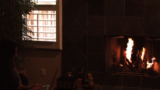
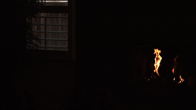
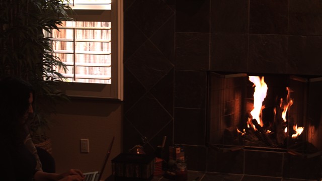
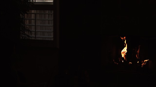
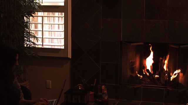
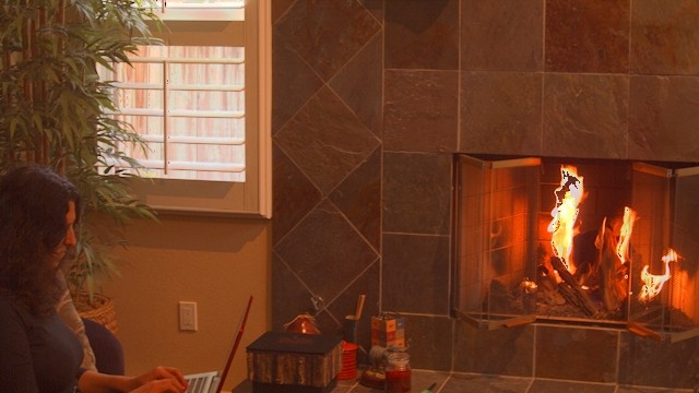
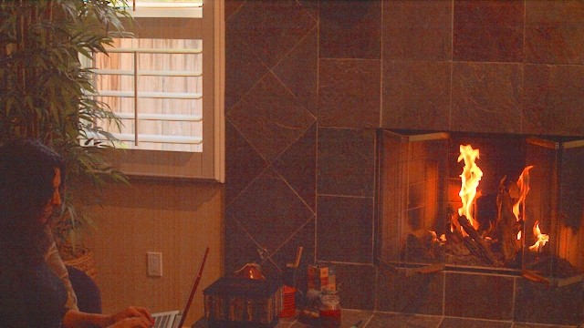
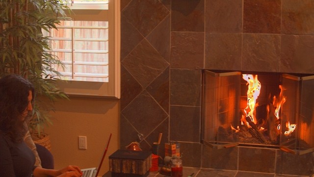
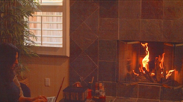
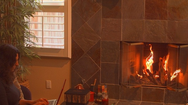
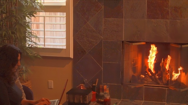
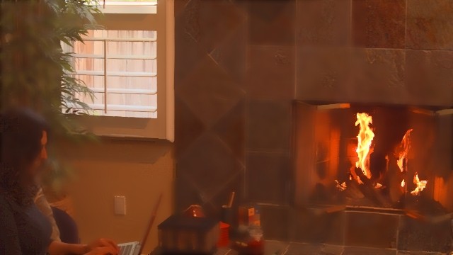
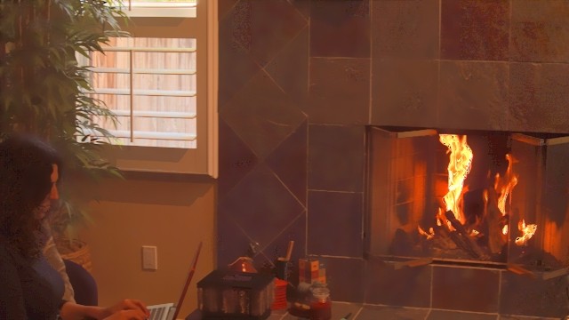
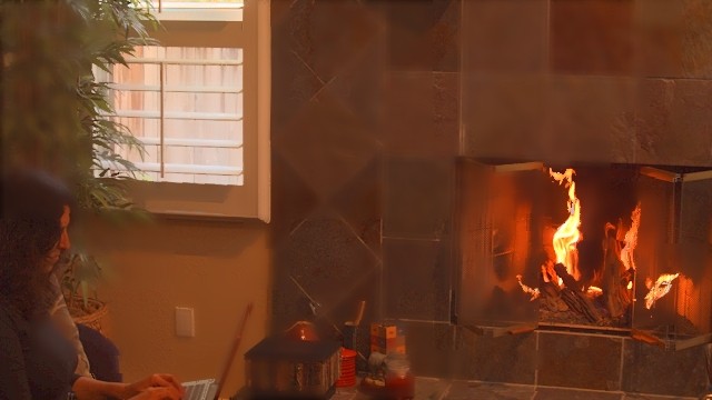
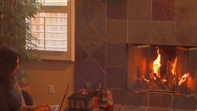
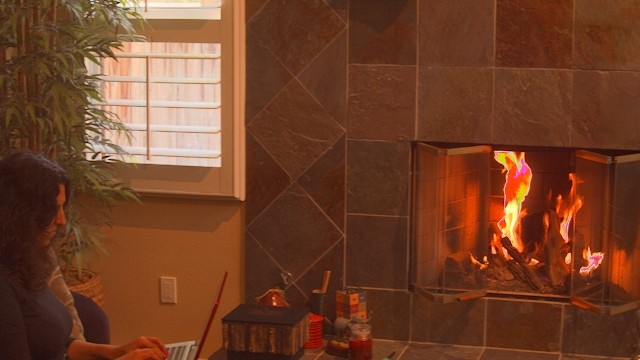
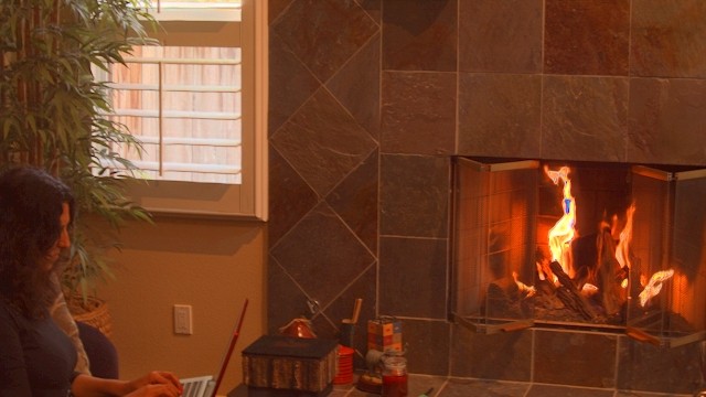
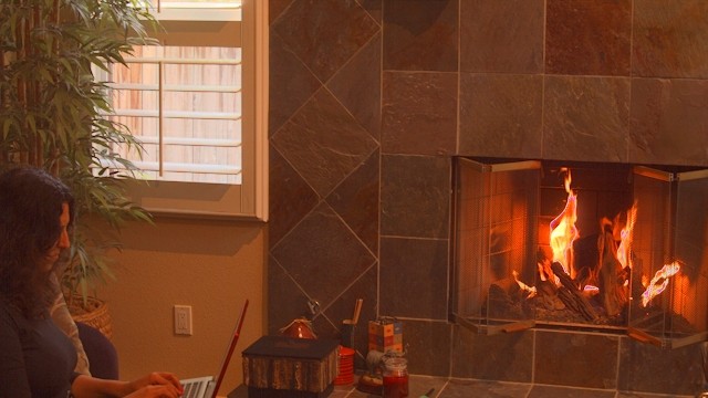
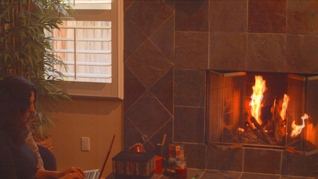
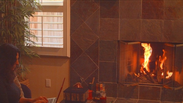
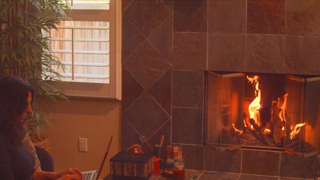
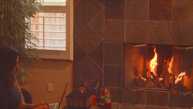
Fig. 5 shows the 4–8th frames of the Fire sequence and the results synthesized by each algorithm. Kang et al.’s algorithm [11] in the second row provides artifacts inside the flames. This is because of its mechanism of compositing the unidirectionally warped frames with bidirectionally warped frames, which may have inconsistent content under mis-registration scenarios. Mangiat and Gibson’s algorithm [17] in the third row performs better than Kang et al.’s, but it still produces artifacts in the flame, as a consequence of mis-registration. For example, it severely blurs the facade of the fireplace of 5th and 7th frames, since its HDR filtering may produce blurred results in the case of mis-registration. Kalantari et al.’s algorithm [19] in the fourth row preserves the shape of flames but introduces color artifacts due to the failure of correspondences estimation. On the contrary, the MAP-HDR algorithm in the fifth row most faithfully renders the video frames with only mild artifacts, which are not even noticeable in the resulting videos.

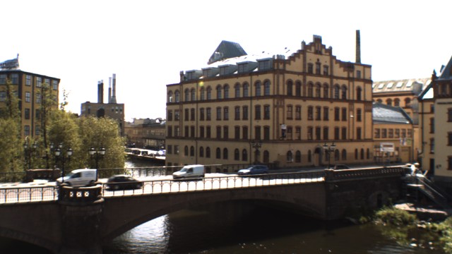
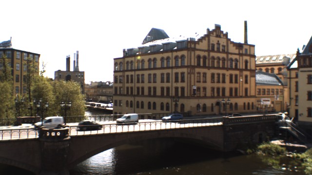
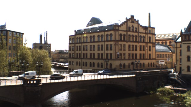
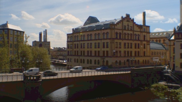
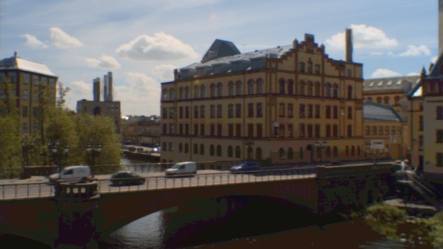
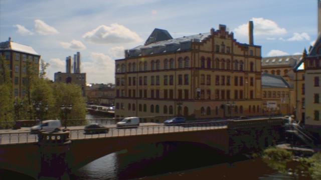
Fig. 6 shows the 3–7th frames of the Bridge2 sequence with synthesized results. Kang et al.’s algorithm works well for the frames with low exposures, whereas it produces severe artifacts for the others. Frames with low exposures usually have few saturated regions, and in such frames Kang et al.’s algorithm maintains most of the original content. However, when a frame has rich saturation, severe artifacts around edges are brought in from bidirectionally warped frames, especially in cases of mis-registrations. Mangiat and Gibson’s algorithm alleviates the artifacts via HDR filtering at the cost of blurring artifacts, e.g., on the facets of the buildings in the 4th and 6th frames. Kalantari et al.’s method distorts the edges of buildings, and also distorts the color in the facet of the bridge. In contrast, we can see that the MAP-HDR algorithm produces higher-quality HDR frames without noticeable artifacts.

Figs. 7–9 compare magnified parts of the results on the Hallway2, ParkingLot, and Students sequences, respectively. In Fig. 7, Kang et al.’s method [11] does not noticeably distort the objects in the 146th frame, while it blends the tower in the 142th frame. Moreover, it introduces noticeable color artifacts. This is because of mis-registration in the bidirectionally warped frames and color inconsistencies in the unidirectionally warped frames. Mangiat and Gibson’s algorithm [17] and Kalantari et al.’s algorithm [19] both introduce visible artifacts. In particular, they both distort the tower of the building. This is due to the failure of optical flow in saturated regions. In the original LDR frames with long exposures, the tower belongs to saturated regions, and optical flow fails to accurately estimate its correspondences. Therefore, both Mangiat and Gibson’s and Kalantari et al.’s algorithms fail to provide high-quality frames, since they both rely on the accuracy of optical flow. In contrast, the MAP-HDR algorithm well preserves the original shape of the tower due to the robustness of the proposed kernel regression scheme discussed in Section III-C.

In Fig. 8, Kang et al.’s algorithm preserves the shape of the van but introduces severe color artifacts in the front of the van because of the inconsistencies between bidirectionally warped frames and unidirectionally warped ones. Mangiat and Gibson’s algorithm provides ghosting artifacts near the tail of the van and erodes the text on the van in the 51th frame due to mis-registration. Kalantari et al.’s algorithm distorts the shape of the van, since its patch-based search fails to fill the saturated region faithfully with content from neighboring frames. In comparison, the MAP-HDR algorithm yields HDR frames without object distortions or ghosting artifacts, while its mild blurring effect is generally unnoticeable in the resulting video.

Fig. 9 compares the synthesized results on the Students sequence, which contains large object motions. Kang et al.’s algorithm [11] provides severe artifacts, e.g., white pixels on a student’s body. Mangiat and Gibson’s algorithm [17] yields clearly visible blurring artifacts, especially around students’ legs and feet, where there are complex and large object motions. Kalantari et al.’s algorithm [19] distorts the shape of the moving objects, e.g., the students’ legs in the 11th frame are shrunk. Moreover, these distortions result in temporal incoherences. In contrast, the MAP-HDR algorithm produces higher-quality results with significantly less artifact both spatially and temporally by employing the multiscale locally adaptive kernel regression.

(a)

(b)

(c)

(d)

(e)

​  ​  ​  ​

(a) Ground truth

(b) Kang et al. [11]

(c) Mangiat and Gibson [17]

(d) Kalantari et al. [19]

(e) MAP-HDR

​  ​  ​  ​

Figure 7: Synthesized results of the 142th frame (top row) and 146th frame (bottom row) on the Hallway2 sequence [4].

(a)

(b)

(c)

(d)

(e)

​  ​  ​  ​

(a) Ground truth

(b) Kang et al. [11]

(c) Mangiat and Gibson [17]

(d) Kalantari et al. [19]

(e) MAP-HDR

​  ​  ​  ​

Figure 8: Synthesized results of the 51th frame (top row) and 53th frame (bottom row) on the ParkingLot sequence [32].

(a)

(b)

(c)

(d)

(e)

​  ​  ​  ​

(a) Ground truth

(b) Kang et al. [11]

(c) Mangiat and Gibson [17]

(d) Kalantari et al. [19]

(e) MAP-HDR

​  ​  ​  ​

Figure 9: Synthesized results for the 11th and 37th frames of the Students sequence [4].

(a)

(b)

(c)

(d)

(e)

​  ​  ​  ​

(a) Input

(b) Kang et al. [11]

(c) Mangiat and Gibson [17]

(d) Kalantari et al. [19]

(e) MAP-HDR

​  ​  ​  ​

Figure 10: Synthesized results of the 106th frame on the ThrowingTowel sequence [19] (top row) and the 16th frame of the WavingHands sequence [19] (bottom row).

While our method can do well in a wide variety of scenarios, there is a breaking point in terms of the amount of motion permissible between frames. Fig. 10 shows two such examples for the ThrowingTowel and WavingHands sequences [19], respectively. For both sequences, Kang et al.’s algorithm and MAP-HDR in Figs. 10(b) and (e), respectively, produce ghosting artifacts. Because of large displacements, even after pyramidal decomposition, some corresponding pixels cannot be brought into a common local block, and thus neither optical flow nor kernel regression can find correct correspondences. Mangiat et al.’s algorithm in Fig. 10(c) provides significant amounts of artifacts, e.g., on the moving arm and the towel in ThrowingTowel and the waving hands in WavingHands, due to the limitation of optical flow in handling large motions. On the other hand, Kalantari et al.’s algorithm in Fig. 10(d) produces the least amount of artifacts. This is because their algorithm employs the PatchMatch algorithm [38] that is capable of handling huge displacements. By far, Kalantari et al.’s algorithm is the only one capable of generating high-quality videos in presence of huge motions, while our algorithm performs the best for reasonably large motions. However, notice that the proposed MAP-HDR requires substantially lower computational complexity than Kalantari et al.’s algorithm as will be discussed in Section V-C.

V-B Objective Video Quality Assessment

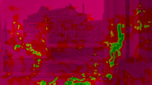
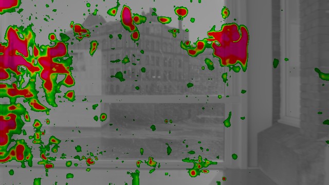
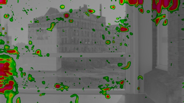
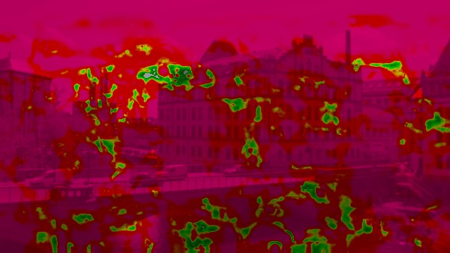
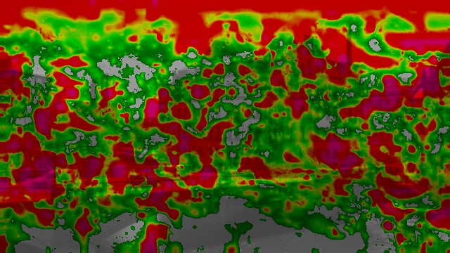
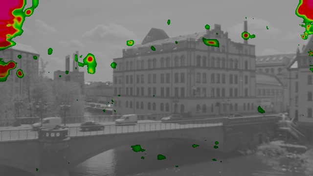
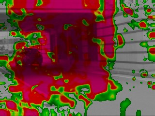
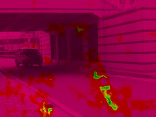
In addition to the subjective evaluation, we compare the MAP-HDR algorithm with the state-of-the-art algorithms using five objective quality metrics: dynamic range independent video quality metric (DRIVQM) [39], logPSNR, perceptually uniform extension to PSNR (puPSNR) [40], high dynamic range-visible difference predictor (HDR-VDP) [41, 42], and high dynamic range-visual quality metric (HDR-VQM) [43]. DRIVQM for each frame estimates the probability that the differences between two frames are to be noticed by a careful viewer in each local region. The logPSNR and puPSNR metrics are extensions of the peak signal-to-noise ratio (PSNR) by taking into account the nonlinear perception of the human visual system to real-world luminance. HDR-VDP estimates the probability at which an average human observer will detect differences between the reference and the query images. In this work, we use the $Q$ correlate of its version 2.2.1 [42]. HDR-VQM predicts the reconstruction quality of the HDR videos using perceptually uniform encoding, sub-band decomposition, short- and long-term spatiotemporal pooling, and the color information of the frames. Note that only DRIVQM and HDR-VQM are dedicated to HDR video quality assessment, whereas the others are developed for still images. Also, because these metrics require the original HDR data as reference, we evaluate the performance only on Bridge2, Hallway2, ParkingLot, and Students.

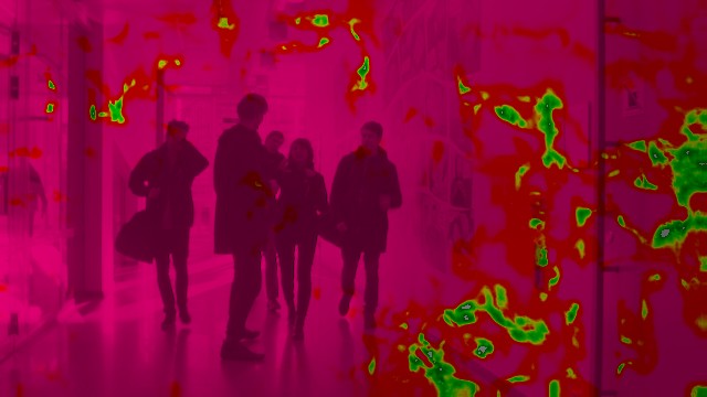
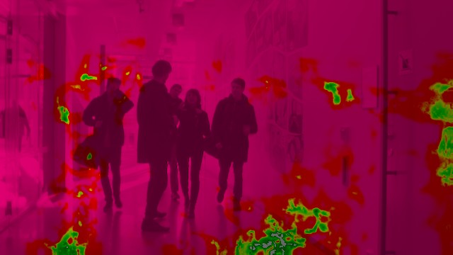
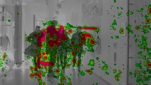
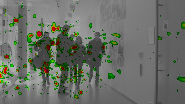
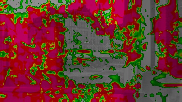
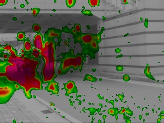
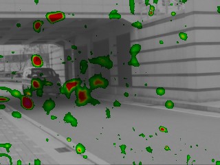
Fig. 11 compares the selected frames of the DRIVQM assessment results on the test sequences. Kang et al.’s algorithm in Fig. 11(a) provides severe visible differences, especially on the Bridge2 and Students sequences, since it composes parts of two different frames together. Mangiat and Gibson’s algorithm in Fig. 11(b) produces visible differences throughout the frames on the Hallway2, ParkingLot, and Studnets sequences, since its HDR filtering severely blurs the whole frame. Kalantari et al.’s algorithm in Fig. 11(c) produces much lower visible differences on the Hallway2 and Brigde2 sequences but poor results on the ParkingLot and Students sequences. On the contrary, we can see that the MAP-HDR algorithm in Fig. 11(d) produces high-quality video results with significantly fewer visible differences than all state-of-the-art algorithms.

Hallway2

(a)

(b)

(c)

(d)

​  ​  ​

Bridge2

(e)

(f)

(g)

(h)

​  ​  ​

ParkingLot

(i)

(j)

(k)

(l)

​  ​  ​

Students

(a) Kang et al. [11]

(b) Mangiat and Gibson [17]

(c) Kalantari et al. [19]

(d) MAP-HDR

​  ​  ​

(e)

Figure 11: DRIVQM assessment on the 140th frame of Hallway2 (top row), the 10th frame of Bridge2 (second row), the 65th frame of ParkingLot (third row), and the 21st frame of Students (bottom row). The colormap depicts the predicted visible differences, i.e., the estimated probability shown in (e), that an observer would notice the differences between the synthesized frames and the references.

TABLE II: Objective assessment of the HDR video synthesis performance using four metrics: logPSNR, puPSNR [40], HDR-VDP [41, 42], and HDR-VQM [43]. Bold-faced numbers denote the highest scores for each metric on each sequence. For all metrics, higher values indicate better quality.

	logPSNR				puPSNR				HDR-VDP				HDR-VQM
	Bridge2	Hallway2	ParkingLot	Students	Bridge2	Hallway2	ParkingLot	Students	Bridge2	Hallway2	ParkingLot	Students	Bridge2	Hallway2	ParkingLot	Students
Kang et al.	25.56	34.06	12.78	17.23	40.66	33.88	23.57	18.81	59.26	59.22	51.02	37.58	0.7435	0.7417	0.7829	0.5852
Mangiat and Gibson	31.85	35.06	29.89	22.66	44.53	35.18	34.19	26.54	61.56	57.91	55.78	50.07	0.8906	0.6913	0.3880	0.5665
Kalantari et al.	36.01	34.98	29.30	21.20	45.56	35.26	38.11	25.47	60.09	62.91	65.92	51.21	0.9446	0.8840	0.7904	0.6677
MAP-HDR	36.48	35.81	31.05	20.69	48.05	36.08	36.93	24.96	59.33	63.91	66.07	51.06	0.9863	0.9242	0.8418	0.6518

Table II quantitatively compares the reconstruction performance of the MAP-HDR algorithm with those of the state-of-the-art algorithms over four test sequences. For each metric on each sequence, the highest scores that indicate the best results are bold-faced. First, logPSNR and puPSNR measure the quality of pixel value reconstruction. Since the proposed MAP-HDR effectively captures motion information via the multiscale adaptive kernel regression algorithm, it provides the highest or close to highest scores on all the test videos in terms of logPSNR and puPSNR, except that it provides the third highest scores on Students. Second, HDR-VDP and HDR-VQM estimate perceptual differences between two videos. On Bridge2, Hallway2, and ParkingLot, the proposed MAP-HDR provides the best performance in terms of both HDR-VDP and HDR-VQM, except for Bridge2 where it provides the third highest HDR-VDP score. We notice that the Students video contains a local regions with extremely high dynamic range of irradiance values, and fitting data with large variations is an inherent limitation of polynomial regression. Therefore, the MAP-HDR provides lower scores on the Students video, although it provides the best visual quality as shown in Fig. 9. Nevertheless, MAP-HDR achieves comparable scores with other algorithms. To summarize, capturing both local structure and temporal motion by solving optimization problems effectively, the proposed MAP-HDR provides overall high-quality videos in these quality metrics.

V-C Computational Complexity Analysis

TABLE III: Comparison of the computational complexities. $N$ and $N_{f}$ denote the number of pixels in a frame and foreground parts, respectively, $P$ is the block sizes (different in each algorithm), $M$ denotes the number of parameters in the kernel regression, $J_{\mathrm{SOR}}$ and $J_{\mathrm{BFGS}}$ are the iteration numbers in the SOR and BFGS procedures, respectively, and $J_{\mathrm{MAX}}=\max\{J_{\mathrm{SOR}},J_{\mathrm{O}}J_{\mathrm{MC}}\}$, where $J_{\mathrm{O}}$ and $J_{\mathrm{MC}}$ denote the number of outer loops and matrix completion iterations in MAP-HDR, respectively. $J_{\mathrm{REC}}$ denotes the number of outer iterations in Kalantari’s algorithm. We also include typical parameter settings and a numerical comparison against a $640\times 480$ gray image, giving $N=307200$, and we let $N_{f}=0.05N=15360$.

	Kang et al.	Mangiat and Gibson	Kalantari et al.	MAP-HDR
Computational Complexity	$\mathcal{O}(P^{2}N)$	${\mathcal{O}}(P^{2}N)$	$\mathcal{O}(J_{\mathrm{REC}}P^{2}N\log N+J_{\mathrm{SOR}}N)$	$\mathcal{O}(N_{f}J_{\mathrm{BFGS}}M^{2}P^{2}+J_{\mathrm{MAX}}N)$
Typical parameter settings	$P=5$	$P=16$	$P=7,J_{\mathrm{REC}}=15$	$P=7,J_{\mathrm{BFGS}}=10,M=10,J_{\mathrm{MAX}}=500$
Resulting asymptotic costs	$7.68\times 10^{6}$	$7.86\times 10^{7}$	$4.12\times 10^{9}$	$7.63\times 10^{8}$

We analyze the computational complexity of synthesizing HDR videos with an $N$-pixel frame. For Kang et al.’s algorithm [11], gradient calculation and image warping via linear interpolation are linear in complexity, which is much lower than other parts of the algorithm, and we hereafter omit their contributions. The critical part of Kang et al.’s algorithm is hierarchical computation of Lucas-Kanade optical flow [12], which has a complexity of $\mathcal{O}(P^{2}N)$, where $P\times P$ is the window size for computing the local structure tensor matrix. Thus, the complexity of Kang et al.’s algorithm is $\mathcal{O}(P^{2}N)$.

Mangiat and Gibson’s algorithm [17] involves two critical parts: block-based motion estimation and HDR filtering. The former has a complexity of $\mathcal{O}(P^{2}N)$ [44], where $P\times P$ is the block size for block matching. The latter has the same complexity as bilateral filtering, i.e., $\mathcal{O}(P^{2}N)$. Thus, Mangiat and Gibson’s algorithm has an overall complexity of $\mathcal{O}(P^{2}N)$.

We compute the complexity of Kalantari et al.’s algorithm [19] by dividing it into three steps as follows.

1. Initial motion estimation: The critical part of this step is optical flow estimation [13], which mainly involves successive over-relaxation (SOR) iterations for solving linear systems. Since each iteration is linear in $N$, the complexity of this step is $\mathcal{O}(J_{\mathrm{SOR}}N)$, where $J_{\mathrm{SOR}}$ denotes the number of SOR iterations.

2. Search window map computation: This step consists of running PatchMatch [38] iteratively for the correspondence estimation. Since PatchMatch has a complexity of $\mathcal{O}(P^{2}N\log N)$ [38] for $P\times P$ patches, the complexity of this step is also $\mathcal{O}(P^{2}N\log N)$.

3. HDR video reconstruction: This is an iterative procedure, and each iteration consists of two steps, i.e., SearchVote and AlphaBlend. In the SearchVote procedure, PatchMatch is executed to find correspondences between reference frame and neighboring frames, which is of $\mathcal{O}(P^{2}N\log N)$ complexity, while AlphaBlend merges aligned frames together, which is of $\mathcal{O}(N)$ complexity. Overall, the complexity is $\mathcal{O}(J_{\mathrm{REC}}(P^{2}N\log N+N))=\mathcal{O}(J_{\mathrm{REC}}P^{2}N\log N)$, where $J_{\mathrm{REC}}$ is the number of outer iterations.

Therefore, the complexity of Kalantari et al.’s algorithm is $\mathcal{O}(J_{\mathrm{REC}}P^{2}N\log N+J_{\mathrm{SOR}}N)$.

The MAP-HDR algorithm consists of two stages: matrix completion for computing the background parts and kernel regression for computing the foreground parts. The first stage turns out to be of $\mathcal{O}(J_{\mathrm{O}}J_{MC}N)$ complexity, where $J_{MC}$ and $J_{\mathrm{O}}$ denote the number of iterations in the matrix completion step [45] and the number of outer loops, respectively. Thanks to the low-rank property of the background matrix (the rank is at most $3$), the QR decomposition procedure becomes trivial as noted in [45], and hence the complexity of each iteration is linear in $N$. The critical step of the second stage is the BFGS optimization in (28), whose critical step is in turn the computation of ${\bf J}$ in (29), which is of complexity $\mathcal{O}(M^{2}P^{2})$, where $M$ and $P$ are the number of parameters for kernel regression and the width of local sample block, respectively. Therefore, the second stage is of complexity $\mathcal{O}(N_{f}J_{\mathrm{BFGS}}M^{2}P^{2})$, where $N_{f}$ and $J_{\mathrm{BFGS}}$ denote the number of foreground pixels and the number of iterations in the BFGS optimization step, respectively. In addition, the optical flow estimation [13] in the pyramidal implementation is of complexity $\mathcal{O}(J_{\mathrm{SOR}}N)$ as in Kalantari et al.’s algorithm. Overall, the complexity of the MAP-HDR algorithm is $\mathcal{O}(N_{f}J_{\mathrm{BFGS}}M^{2}P^{2}+J_{\mathrm{MAX}}N)$, where $J_{\mathrm{MAX}}=\max\{J_{\mathrm{SOR}},J_{\mathrm{O}}J_{\mathrm{MC}}\}$.

We summarize the complete complexities in Table III. We see that both Kang et al.’s and Mangiat and Gibson’s methods have relatively lower complexities; however, both methods are prone to introducing serious artifacts when mis-registration happens as shown in Figs 5–8. Let us compare complexities of Kalantari et al.’s algorithm and the MAP-HDR algorithm quantitatively. For Kalantari et al.’s algorithm with $P=7$, summing up $J_{\mathrm{REC}}$’s in each scale gives an equivalent $J_{\mathrm{REC}}\approx 15$, and usually $J_{\mathrm{SOR}}N\ll J_{\mathrm{REC}}P^{2}N\log N$. In contrast, in the MAP-HDR algorithm, typically $J_{\mathrm{BFGS}}\leq 10$, $M=10$, $P=7$, $N_{f}\ll N$, and $J_{\mathrm{MAX}}$ typically varies from several hundreds to a thousand. Because our algorithm produces better results than competing methods in most (but not all) cases, it achieves a better complexity-performance trade-off.

VI Conclusion

We develop a MAP estimation-based approach to HDR video synthesis from a series of LDR frames taken with alternating exposure times. By choosing physically meaningful priors, e.g., low-rank background and the Ising model, the MAP estimation can be reduced to a tractable optimization problem, the solution to which provides aligned background regions as well as foreground irradiance that implicitly captures motion information. To capture motion information of the foreground regions, we further develop a multiscale adaptive kernel regression algorithm. Finally, HDR frame synthesis simply follows by combining the foreground with the background. Experimental results on challenging video sequences demonstrate the effectiveness of our algorithm in obtaining high-quality HDR video sequences. Some of the important directions for future work are to incorporate more accurate noise models, such as those mentioned in [46, 47], and to extend the framework towards handling very large object and camera motion as in [19].

Appendix A Derivation of the Estimation in (17)

Since ${\bf S}$ is the support of ${\bf F}$, by the Bayes formula, the posterior probability $f({\bf S},{\bf B},{\bf F}|{\bf D})=\frac{f({\bf D},{\bf B},{\bf F}|{\bf S})f({\bf S})}{f({\bf D})}$ in (13) is given by

$$f({\bf S},{\bf B},{\bf F}|{\bf D}) =f({\bf D},{\bf B},{\mathcal{P}}_{\bf S}({\bf F})|{\bf S})f({\bf S})$$

$$=f({\mathcal{P}}_{{\bf S}^{\mathsf{c}}}({\bf D}),{\mathcal{P}}_{\bf S}({\bf D}),{\bf B},{\mathcal{P}}_{\bf S}({\bf F})|{\bf S})f({\bf S}),$$

where we use the identity ${\bf D}={\mathcal{P}}_{{\bf S}^{\mathsf{c}}}({\bf D})+{\mathcal{P}}_{\bf S}({\bf D})$. Then, based on the assumption that the foreground ${\bf F}$ and background ${\bf B}$ are independent, from (14) and (15), we have

$$f({\bf S},{\bf B},{\bf F}|{\bf D}) =f({\mathcal{P}}_{{\bf S}^{\mathsf{c}}}({\bf D}),{\bf B}|{\bf S})f({\mathcal{P}}_{\bf S}({\bf F}),{\mathcal{P}}_{{\bf S}}({\bf D})|{\bf S})f({\bf S})$$

$$=f({\mathcal{P}}_{{\bf S}^{\mathsf{c}}}({\bf D}),{\bf B})f({\mathcal{P}}_{\bf S}({\bf F}),{\mathcal{P}}_{{\bf S}}({\bf D}))f({\bf S}).$$ (31)

Taking the logarithm of both sides of (31) yields

$$\log f({\bf S},{\bf B},{\bf F}|{\bf D}) =\log f({\mathcal{P}}_{{\bf S}^{\mathsf{c}}}({\bf D}),{\bf B})$$

$${}\quad+\log f({\mathcal{P}}_{\bf S}({\bf F}),{\mathcal{P}}_{{\bf S}}({\bf D}))+\log f({\bf S})$$

$$=\log f({\mathcal{P}}_{{\bf S}^{\mathsf{c}}}({\bf D})|{\bf B})+\log f({\bf B})$$

$${}\quad+\log f({\mathcal{P}}_{\bf S}({\bf F}),{\mathcal{P}}_{\bf S}({\bf D}))+\log f({\bf S}).$$

Finally, since

$$\underset{{\bf S},{\bf B},{\bf F}}{\arg\max}\;f({\bf S},{\bf B},{\bf F}|{\bf D})=\underset{{\bf S},{\bf B},{\bf F}}{\arg\max}\;\log f({\bf S},{\bf B},{\bf F}|{\bf D}),$$

we obtain (17).

Appendix B Derivation of the Gradient $\nabla\mathcal{C}$ in (29)

To illustrate, we consider each term in (28) separately as

$$\mathcal{C}_{1} :=({\bf y}-{\bf X}\widehat{\bm{\beta}})^{T}\bm{\Lambda}({\bf y}-{\bf X}\widehat{\bm{\beta}})+({\bf y}-t{\bf 1})^{T}\widetilde{\bm{\Lambda}}({\bf y}-t{\bf 1}),$$

$$\mathcal{C}_{2} :=\|\widehat{\bm{\beta}}\|_{2}^{2},$$

$$\mathcal{C}_{3} :=\|{\bf R}\|_{F}^{2}.$$

As in (28), let ${\bf T}=({\bf X}^{T}\bm{\Lambda}{\bf X}+\varepsilon{\bf I})^{-1}{\bf X}^{T}$ and ${\bf J}={\bf X}{\bf T}$. Then, since $\mathrm{d}{{\bf A}^{-1}}=-{\bf A}^{-1}(\mathrm{d}{\bf A}){\bf A}^{-1}$ [48], we have

$$\mathrm{d}{\bf T} =-({\bf X}^{T}\bm{\Lambda}{\bf X}+\varepsilon{\bf I})^{-1}{\bf X}^{T}(\mathrm{d}\bm{\Lambda}){\bf X}({\bf X}^{T}\bm{\Lambda}{\bf X}+\varepsilon{\bf I})^{-1}{\bf X}^{T}$$

$$=-{\bf T}(\mathrm{d}\bm{\Lambda}){\bf J}.$$

Therefore,

$$\mathrm{d}\widehat{\bm{\beta}} =-{\bf T}(\mathrm{d}\bm{\Lambda}){\bf J}\bm{\Lambda}{\bf y}+{\bf T}(\mathrm{d}\bm{\Lambda}){\bf y}$$

$$={\bf T}(\mathrm{d}\bm{\Lambda})({\bf y}-{\bf X}\widehat{\bm{\beta}})$$

and $\mathrm{d}\widehat{y}_{i}={\bf e}_{i}^{T}\mathrm{d}({\bf X}\widehat{\bm{\beta}})=\sum_{j\in\mathcal{G}}J_{ij}(y_{j}-\widehat{y}_{j})\mathrm{d}k_{j}$. Also, we have

$$\mathrm{d}J_{ii} ={\bf e}_{i}^{T}(\mathrm{d}{\bf J}){\bf e}_{i}=-{\bf e}_{i}^{T}{\bf J}(\mathrm{d}\bm{\Lambda}){\bf J}{\bf e}_{i}=-\sum_{j\in\mathcal{G}}J_{ij}^{2}\mathrm{d}k_{j}.$$

Next, by the chain rule [48], we can obtain

$$\mathrm{d}k_{i} =k_{i}\mathrm{d}\!\left(-\frac{1}{2}({\bf x}_{i}-{\bf x})^{T}{\bf R}^{T}{\bf R}({\bf x}_{i}-{\bf x})\right)$$

$$=-k_{i}\left\langle{\bf R}({\bf x}_{i}-{\bf x})({\bf x}_{i}-{\bf x})^{T},\mathrm{d}{\bf R}\right\rangle\!,$$

where $\langle{\bf A},{\bf B}\rangle:=\mathrm{tr}({\bf A}^{T}{\bf B})$ denotes the Frobenius inner product of two matrices ${\bf A}$ and ${\bf B}$. Similarly, for $\tilde{k}_{i}$,

$$\mathrm{d}\tilde{k}_{i} =-\tilde{k}_{i}\left\langle{\bf R}({\bf x}_{i}-{\bf x})({\bf x}_{i}-{\bf x})^{T},\mathrm{d}{\bf R}\right\rangle\!.$$

Thus,

$$\mathrm{d}\mathcal{C}_{1} =\mathrm{d}\!\left\{\sum_{i}k_{i}(y_{i}-\widehat{y}_{i})^{2}+\tilde{k}_{i}(y_{i}-t)^{2}\right\}$$

$$=\sum_{i}(y_{i}-\widehat{y}_{i})^{2}\mathrm{d}k_{i}+k_{i}\mathrm{d}(y_{i}-\widehat{y}_{i})^{2}+(y_{i}-t)^{2}\mathrm{d}\tilde{k}_{i}$$

$$=\left\langle\!{\bf R}\Bigg{\{}2\sum_{i,j}k_{i}k_{j}J_{ij}(y_{i}-\widehat{y}_{i})(y_{j}-\widehat{y}_{j})({\bf x}_{j}-{\bf x})({\bf x}_{j}-{\bf x})^{T}\right.$$

$${}\quad\left.-\sum_{i}\left(k_{i}z_{i}^{2}+\tilde{k}_{i}\tilde{z}_{i}^{2}\right)({\bf x}_{i}-{\bf x})({\bf x}_{i}-{\bf x})^{T}\Bigg{\}}\!,\mathrm{d}{\bf R}\right\rangle\!.$$

Also, we can derive $\mathrm{d}\mathcal{C}_{2}$ and $\mathrm{d}\mathcal{C}_{3}$ as

$$\mathrm{d}\mathcal{C}_{2} =\left\langle-2{\bf R}\sum_{i,j}\widehat{\beta}_{i}k_{j}T_{ij}(y_{j}-\widehat{y}_{j})({\bf x}_{j}-{\bf x})({\bf x}_{j}-{\bf x})^{T},\mathrm{d}{\bf R}\right\rangle$$

and $\mathrm{d}\mathcal{C}_{3}=\left\langle 2{\bf R},\mathrm{d}{\bf R}\right\rangle$, respectively.

Since $\mathrm{d}\mathcal{C}=\mathrm{d}\mathcal{C}_{1}+\lambda\mathrm{d}\mathcal{C}_{2}+\mu\mathrm{d}\mathcal{C}_{3}$, and since ${\bf R}$ is upper triangular, so is $\mathrm{d}{\bf R}$; and $\nabla\mathcal{C}$ is thus given by (29).

References

- [1] E. Reinhard, G. Ward, S. Pattanaik, P. Debevec, W. Heidrich, and K. Myszkowski, High Dynamic Range Imaging: Acquisition, Display, and Image-Based Lighting, 2nd ed. San Mateo, CA: Morgan Kaufmann Publishers, 2010.
- [2] S. K. Nayar and V. Branzoi, “Adaptive dynamic range imaging: Optical control of pixel exposures over space and time,” in Proc. IEEE Int. Conf. Comput. Vis., Oct. 2003, pp. 1168–1175.
- [3] M. D. Tocci, C. Kiser, N. Tocci, and P. Sen, “A versatile HDR video production system,” ACM Trans. Graphics, vol. 30, no. 4, pp. 41:1–10, Jul. 2011.
- [4] J. Kronander, S. Gustavson, G. Bonnet, A. Ynnerman, and J. Unger, “A unified framework for multi-sensor HDR video reconstruction,” Signal Process.: Image Commun., vol. 29, no. 2, pp. 203–215, Feb. 2014.
- [5] P. E. Debevec and J. Malik, “Recovering high dynamic range radiance maps from photographs,” in Proc. ACM SIGGRAPH, Aug. 1997, pp. 369–378.
- [6] P. Sen, N. K. Kalantari, M. Yaesoubi, S. Darabi, D. B. Goldman, and E. Shechtman, “Robust patch-based HDR reconstruction of dynamic scenes.” ACM Trans. Graphics, vol. 31, no. 6, pp. 203:1–11, Nov. 2012.
- [7] J. Hu, O. Gallo, K. Pulli, and X. Sun, “HDR deghosting: How to deal with saturation?” in Proc. IEEE Conf. Comput. Vis. Pattern Recognit., Jun. 2013, pp. 1163–1170.
- [8] C. Lee, Y. Li, and V. Monga, “Ghost-free high dynamic range imaging via rank minimization,” IEEE Signal Process. Lett., vol. 21, no. 9, pp. 1045–1049, Sep. 2014.
- [9] T.-H. Oh, J.-Y. Lee, Y.-W. Tai, and I. S. Kweon, “Robust high dynamic range imaging by rank minimization,” IEEE Trans. Pattern Anal. Mach. Intell., vol. 37, no. 6, pp. 1219–1232, Jun. 2015.
- [10] O. T. Tursun, A. O. Akyüz, A. Erdem, and E. Erdem, “The state of the art in HDR deghosting: A survey and evaluation,” Comput. Graph. Forum, vol. 34, no. 2, pp. 683–707, May 2015.
- [11] S. B. Kang, M. Uyttendaele, S. Winder, and R. Szeliski, “High dynamic range video,” ACM Trans. Graphics, vol. 22, no. 3, pp. 319–325, Jul. 2003.
- [12] B. D. Lucas and T. Kanade, “An iterative image registration technique with an application to stereo vision,” in Proc. 7th Int. Joint Conf. Artificial Intell., 1981, pp. 674–679.
- [13] C. Liu, “Beyond pixels: Exploring new representations and applications for motion analysis,” Ph.D. dissertation, Massachusetts Institute of Technology, Cambridge, MA, May 2009.
- [14] J. Unger and S. Gustavson, “High-dynamic-range video for photometric measurement of illumination,” in Proc. SPIE Sensors, Cameras, and Systems for Scientific/Industrial Applications VIII, vol. 6501, Feb. 2007, pp. 6501:1–10.
- [15] S. Mangiat and J. Gibson, “High dynamic range video with ghost removal,” in Proc. SPIE Applications of Digital Image Processing XXXIII, vol. 7798, Aug. 2010, pp. 779 812:1–8.
- [16] B. K. Horn and B. G. Schunck, “Determining optical flow,” Artificial Intell., vol. 17, pp. 185–203, Apr. 1981.
- [17] S. Mangiat and J. Gibson, “Spatially adaptive filtering for registration artifact removal in HDR video,” in IEEE Int. Conf. Image Process., Sep. 2011, pp. 1317–1320.
- [18] ——, “Inexpensive high dynamic range video for large scale security and surveillance,” in Proc. Int. Conf. Military Commun., Nov. 2011, pp. 1772–1777.
- [19] N. K. Kalantari, E. Shechtman, C. Barnes, S. Darabi, D. B. Goldman, and P. Sen, “Patch-based high dynamic range video,” ACM Trans. Graphics, vol. 32, no. 6, pp. 202:1–8, Nov. 2013.
- [20] Y. Li, C. Lee, and V. Monga, “A MAP estimation framework for HDR video synthesis,” in Proc. IEEE Int. Conf. Image Process., Sep. 2015, pp. 2219–2223.
- [21] H. Takeda, S. Farsiu, and P. Milanfar, “Kernel regression for image processing and reconstruction,” IEEE Trans. Image Process., vol. 16, no. 2, pp. 349–366, Feb. 2007.
- [22] H. Takeda, P. Milanfar, M. Protter, and M. Elad, “Super-resolution without explicit subpixel motion estimation,” IEEE Trans. Image Process., vol. 18, no. 9, pp. 1958–1975, Sep. 2009.
- [23] S. Schaal and C. G. Atkeson, “Constructive incremental learning from only local information,” Neural Computation, vol. 10, no. 8, pp. 2047–2084, Nov. 1998.
- [24] A. Blake, P. Kohli, and C. Rother, Markov Random Fields for Vision and Image Processing. Cambridge, MA: MIT Press, 2011.
- [25] V. Cevher, P. Indyk, L. Carin, and R. G. Baraniuk, “Sparse signal recovery and acquisition with graphical models,” IEEE Signal Process. Mag., vol. 27, no. 6, pp. 92–103, Nov. 2010.
- [26] V. Cevher, M. F. Duarte, C. Hegde, and R. Baraniuk, “Sparse signal recovery using Markov random fields,” in Proc. Neural Inf. Process. Syst., Dec. 2009, pp. 257–264.
- [27] V. Kolmogorov and R. Zabih, “What energy functions can be minimized via graph cuts?” IEEE Trans. Pattern Anal. Mach. Intell., vol. 26, no. 2, pp. 147–159, Feb. 2004.
- [28] S. G. Johnson. The NLopt nonliear optimization package. [Online]. Available: http://ab-initio.mit.edu/nlopt
- [29] J. Nocedal, “Updating quasi-newton matrices with limited storage,” Math. Comput., vol. 35, pp. 773–782, 1980.
- [30] D. C. Liu and J. Nocedal, “On the limited memory BFGS method for large scale optimization,” Math. Program., vol. 45, no. 3, pp. 503–528, Dec. 1989.
- [31] J. Nocedal and S. J. Wright, Numerical Optimization, 2nd ed. New York, NY: Springer, 2006.
- [32] C. Lee and C.-S. Kim, “Rate-distortion optimized layered coding of high dynamic range videos,” J. Vis. Commun. Image R., vol. 23, no. 6, pp. 908–923, Aug. 2012.
- [33] T. Brox, A. Bruhn, N. Papenberg, and J. Weickert, “High accuracy optical flow estimation based on a theory for warping,” in Proc. European Conf. Comput. Vis., May 2004, pp. 25–36.
- [34] A. Bruhn, J. Weickert, and C. Schnörr, “Lucas/Kanade meets Horn/Schunck: Combining local and global optic flow methods,” Int. J. Comput. Vis., vol. 61, no. 3, pp. 211–231, Feb. 2005.
- [35] [Online]. Available: http://www.ece.ucsb.edu/~psen/PaperPages/HDRVideo/HDRVideo_MATLAB_v1.0.zip
- [36] [Online]. Available: http://www.ece.ucsb.edu/~kuochin/release/HDR_MATLAB.zip
- [37] E. Reinhard, M. Stark, P. Shirley, and J. Ferwerda, “Photographic tone reproduction for digital images,” ACM Trans. Graphics, vol. 21, no. 3, pp. 267–276, Jul. 2002.
- [38] C. Barnes, E. Shechtman, A. Finkelstein, and D. B. Goldman, “Patchmatch: A randomized correspondence algorithm for structural image editing,” ACM Trans. Graphics, vol. 28, no. 3, pp. 24:1–11, Jul. 2009.
- [39] T. O. Aydin, M. Čadík, K. Myszkowski, and H.-P. Seidel, “Video quality assessment for computer graphics applications,” ACM Trans. Graphics, vol. 29, no. 6, pp. 161:1–12, Dec. 2010.
- [40] T. O. Aydın, R. Mantiuk, and H.-P. Seidel, “Extending quality metrics to full luminance range images,” in Proc. IS&T/SPIE Human Vision and Electronic Imaging, Feb. 2008, p. 68060B.
- [41] R. Mantiuk, K. J. Kim, A. G. Rempel, and W. Heidrich, “HDR-VDP-2: A calibrated visual metric for visibility and quality predictions in all luminance conditions,” ACM Trans. Graphics, vol. 30, no. 4, pp. 40:1–40:14, Jul. 2011.
- [42] M. Narwaria, R. K. Mantiuk, M. P. D. Silva, and P. L. Callet, “HDR-VDP-2.2: A calibrated method for objective quality prediction of high-dynamic range and standard images,” J. Electronic Imaging, vol. 24, no. 1, p. 010501, Jan. 2015.
- [43] M. Narwaria, M. P. D. Silva, and P. L. Callet, “HDR-VQM: An objective quality measure for high dynamic range video,” Signal Process.: Image Commun., vol. 35, pp. 46–60, Jul. 2015.
- [44] Y. Nie and K.-K. Ma, “Adaptive rood pattern search for fast block-matching motion estimation,” IEEE Trans. Image Process., vol. 11, no. 12, pp. 1442–1449, Dec. 2002.
- [45] Z. Wen, W. Yin, and Y. Zhang, “Solving a low-rank factorization model for matrix completion by a nonlinear successive over-relaxation algorithm,” Math. Prog. Comput., vol. 4, no. 4, pp. 333–361, Jul. 2012.
- [46] S. W. Hasinoff, F. Durand, and W. T. Freeman, “Noise-optimal capture for high dynamic range photography,” in Proc. IEEE Conf. Comput. Vis. Pattern Recognit., Jun. 2010, pp. 553–560.
- [47] M. Granados, B. Ajdin, M. Wand, C. Theobalt, H.-P. Seidel, and H. P. A. Lensch, “Optimal HDR reconstruction with linear digital cameras,” in Proc. IEEE Conf. Comput. Vis. Pattern Recognit., Jun. 2010, pp. 215–222.
- [48] J. R. Magnus and H. Neudecker, Matrix Differential Calculus with Applications in Statistics and Econometrics, 2nd ed. Chichester, UK: John Wiley & Sons, 1999.