Abstract

We study the optimization problem for remote one- and two-qubit state creation via a homogeneous spin-1/2 communication line using the local unitary transformations of the multi-qubit sender and extended receiver. We show that the maximal length of a communication line used for the needed state creation (the critical length) increases with an increase in the dimensionality of the sender and extended receiver. The model with the sender and extended receiver consisting of up to 10 nodes is used for the one-qubit state creation and we consider two particular states: the almost pure state and the maximally mixed one. Regarding the two-qubit state creation, we numerically study the dependence of the critical length on a particular triad of independent eigenvalues to be created, the model with four-qubit sender without an extended receiver is used for this purpose.

I Introduction

The problem of quantum state transfer Bose was studied in many papers. The main purpose of that research is increasing the state-transfer fidelity in long chains. Thus, perfect state transfer is possible in chains with specially adjusted coupling constants governed by the nearest-neighbor XY-Hamiltonian CDEL ; ACDE ; KS , the high probability state transfer (HPST) can be arranged in a simpler way using the boundary controlled chains GKMT ; WLKGGB ; BACVV2010 ; ZO ; BACVV2011 ; ABCVV or the special non-uniform magnetic field DZ . The high-fidelity state transfer along the homogeneous spin chains considered in refs.H ; BOWB is achieved via encoding a one-qubit state into the multi-qubit sender in an optimal way. As an optimization tool, the singular value decomposition (SVD) of a certain matrix was used.

In this paper we consider the remote one-qubit state creation in a homogeneous communication line with a multi-qubit sender. The long distance creation of a needed state is achieved using a pair of optimized local unitary transformations on the sender and receiver sides. This optimization is based on the SVD of a certain matrix whose elements are expressed in terms of transition amplitudes between different nodes of a communication line.

Among the one-qubit creatable states, we consider the almost pure state (in this case we deal with an analogue of high-probability state transfer) and the maximally mixed state (i.e., the state with two equal eigenvalues $\lambda_{1}=\lambda_{2}=\frac{1}{2}$). The interest in the latter state is motivated by the fact BZ_2015 that having the communication line allowing the creation of maximally mixed state we can also create the state with any eigenvalue $\lambda_{1}$ just using the proper choice of the parameters of the sender’s initial state. Hereafter the maximal length allowing the particular state creation is referred to as the critical length $N_{c}$ for this state. Thus, the critical length for the maximally mixed state is also the critical length for the creation of a state with an arbitrary eigenvalue.

We also consider the remote two-qubit state creation. Since this state is multi-parametric one, we restrict ourselves to studying the eigenvalue creation disregarding other parameters of that state. At that, we numerically find the dependence of the critical length $N_{c}$ on the eigenvalues to be created.

The paper is organized as follows. The general protocol of remote state creation using the communication line with multi-qubit sender and extended receiver is given in Sec.II. The optimization is based on SVD. This protocol is applied to the one-qubit state creation in Sec.III where the communication line with the sender and extended receiver of up to 10 nodes is used. We consider the high-probability almost pure state creation and creation of maximally mixed state. The eigenvalue creation of two-qubit receiver is studied in Sec.IV. Conclusions are given in Sec.V. The time optimization and some details of two-qubit state creation are given in Appendix, Sec.VI.

II One-excitation spin dynamics and optimization tool

We proceed with the one-qubit receiver and consider the problem of high-probability pure state creation KZ_2008 ; SAOZ ; BK ; C ; QWL ; B ; JKSS ; SO ; BB ; SJBB and eigenvalue creation BZ_2015 ; BZ_2016 in a long spin-1/2 chain with the $N_{S}$-qubit sender, one-qubit receiver and $N_{R}$-qubit extended receiver, as shown in Fig.1.

Figure 1: The communication line with the $N_{S}$-qubit sender $S$, one-qubit receiver $R$ and $N_{R}$-qubit extended receiver $R^{ext}$.

Hereafter we consider the one-excitation spin dynamics governed by the Hamiltonian $H$ conserving the $z$-projection of the total spin. The evolution of a one-excitation state can be described in the $N$-dimensional space spanned by the following basis vectors:

$$|n\rangle,\;\;n=1,\dots,N,$$ (1)

where $n$ means the state with the $n$th polarized spin. Therefore, the general initial state $|\Psi_{0}\rangle$ of our interest reads:

$$|\Psi_{0}\rangle=\sum_{i=1}^{N_{s}}a_{i}|i\rangle,\;\;\sum_{i=1}^{N_{s}}|a_{i}|^{2}=1.$$ (2)

Its evolution is described by the Lioville equation:

$$|\Psi(t)\rangle=e^{-iH_{1}t}|\Psi_{0}\rangle,$$ (3)

where $H_{1}$ is the $N\times N$ block of the Hamiltonian responsible for the one-excitation evolution. We can diagonalize the Hamiltonian $H_{1}$:

$$H_{1}=We^{-i\Lambda t}W^{+},$$ (4)

where $\Lambda={\mbox{diag}}(\lambda_{1},\dots,\lambda_{N})$ and $W$ are, respectively, the eigenvalue matrix and the matrix of the eigenvectors. If, in addition, we apply the unitary transformation $V$ to the extended receiver at the time instant $t_{0}$, then the obtained state $\Psi^{V}$ reads

$$|\Psi^{V}\rangle=\tilde{V}We^{-i\Lambda t_{0}}W^{+}|\Psi_{0}\rangle.$$ (5)

Here the operator $\tilde{V}$ in the basis (1) has the block-diagonal form, $\tilde{V}={\mbox{diag}}(I_{rest},V)$, where $I_{rest}$ is an $(N-N_{R})$-dimensional identity operator and $V$ is an $N_{R}\times N_{R}$ unitary operator. The state of the one-qubit receiver $\rho^{R}$ is determined by the trace of the state (3) over all other spins:

$$\rho^{R}={\mbox{Tr}}_{1,\dots,N-1}|\Psi^{V}\rangle\langle\Psi^{V}|,$$ (6)

where the trace is taken over all the nodes except the node of the receiver. It is simple to show (see, for instance, ref.BZ_2015 ) that this state has the following diagonal form (represented in the one-qubit basis $|0\rangle$, $|1\rangle$)

$$\rho^{R}=\left(\begin{array}[]{cc}1-|f_{N}|^{2}&0\cr 0&|f_{N}|^{2}\end{array}\right),$$ (9)

where the projection $f_{N}$ is defined as

$$f_{N}=\langle N|\Psi^{V}\rangle,$$ (10)

and the eigenvalues of state (9) read

$$\lambda_{1}=1-|f_{N}|^{2},\;\;\lambda_{2}=|f_{N}|^{2}.$$ (11)

Below we consider the creation of two particular states. The first one is the state maximally approximating the pure state $|N\rangle$ (an analogy of the HPST). More exactly, the state with

$$|f_{N}|^{2}>0.9.$$ (12)

The second state is the maximally mixed state, $\lambda_{1}=\lambda_{2}=\frac{1}{2}$, which corresponds to

$$|f_{N}|^{2}=\frac{1}{2}.$$ (13)

The motivation for studying this state is mentioned in the Introduction. The choice of the above two states and appropriate conditions (12) and (13) support our disregarding the contribution to the initial state (2) from the ground state (i.e., the state without excitations), because this contribution reduces $|f_{N}|$ BZ_2015 .

II.1 Singular-value decomposition as optimization tool

For constructing the desired state we use the optimization method based on the SVD H (see also BZ_2016 ). We give some details of this procedure. The projection $f_{N}$ defined in (10) can be represented as follows:

$$f_{N}=\langle N|\Pi_{R}^{+}V{\mathcal{P}}\Pi_{S}|\Psi_{0}\rangle,\;\;{\mathcal{P}}_{nm}=\sum_{k=1}^{N}W_{(N-N_{R}+n)k}e^{-i\lambda^{H}_{k}t}W_{mk},$$ (14)

$$n=1,\dots,N_{R},\;\;m=1,\dots,N_{S},$$

where we take into account reality of $W$ and use two shorten bases: $|n\rangle_{S}$, $n=1,\dots,N_{S}$ (to enumerate the columns of ${\mathcal{P}}$) and $|n\rangle_{R}$, $n=1,\dots,N_{R}$ (to enumerate the rows of ${\mathcal{P}}$) introduced via the rectangular operators $\Pi_{S}$ ($N_{S}\times N$) and $\Pi_{R}$ ($N_{R}\times N$) by the formulas

$$|n\rangle_{S}=\Pi_{S}|n\rangle,\;\;n=1,\dots,N_{S},\;\;\Pi_{S}|n\rangle=|0\rangle_{S},\;\;n>N_{S},$$ (15)

$$|n\rangle_{R}=\Pi_{R}|N-N_{R}+n\rangle,\;\;n=1,\dots,N_{R},\;\;\Pi_{R}|n\rangle=|0\rangle_{R},\;\;n\leq N-N_{R}.$$

Thus, $\Pi_{S}$ and $\Pi_{R}$ are, respectively, the first $N_{S}$ and the last $N_{R}$ rows of the $N\times N$ identity matrix. SVD of ${\mathcal{P}}$ reads

$${\mathcal{P}}=V^{SVD}\Lambda^{SVD}(U^{SVD})^{+},$$ (16)

where $\Lambda^{SVD}={\mbox{diag}}(\omega_{1},\omega_{2}\dots)$ is the diagonal matrix of singular values. We require that the first singular value is the maximal one. We note two symmetry properties of SVD.

1. SVD is defined up to the phase transformation

   $$(V^{SVD}_{kn},U^{SVD}_{mn})\;\to\;(V^{SVD}_{kn}e^{i\varphi_{n}},U^{SVD}_{mn}e^{i\varphi_{n}}),\;\;\forall\varphi_{n}\in{\mathbb{R}}.$$ (17)

2. The considered system is symmetrical with respect to the reversion of the order of the nodes (the Hamiltonian is symmetrical with respect to the secondary diagonal). Therefore, if we consider the chain with $N_{S}=N_{1}$, $N_{R}=N_{2}$ (${\mathcal{P}}_{1}=V^{SVD}_{1}\Lambda^{SVD}_{1}(U^{SVD}_{1})^{+}$) and the other chain with $N_{S}=N_{2}$, $N_{R}=N_{1}$ (${\mathcal{P}}_{2}=V^{SVD}_{2}\Lambda^{SVD}_{2}(U^{SVD}_{2})^{+}$), then (up to the above phase transformation)

   $$\Lambda^{SVD}_{2}=(\Lambda^{SVD}_{1})^{T},\;\;(V^{SVD}_{2})_{n,m}=(U^{SVD}_{1})^{*}_{N_{1}-n+1,m},\;\;(V^{SVD}_{1})_{n,m}=(U^{SVD}_{2})^{*}_{N_{1}-n+1,m}.$$ (18)

   In particular, if $N_{1}=N_{2}$, then both chains are equivalent and

   $$\Lambda^{SVD}_{1}\equiv\Lambda^{SVD}_{2},\;\;(V^{SVD}_{1})_{n,m}=(V^{SVD}_{2})_{n,m}=(U^{SVD}_{1})^{*}_{N_{1}-n+1,m}=(U^{SVD}_{2})^{*}_{N_{1}-n+1,m},$$ (19)

   where $*$ means complex conjugation.

Next, we introduce the $N_{S}\times N_{S}$ unitary operator $U$ of the sender such that $\Pi_{S}|\Psi_{0}\rangle=U\Pi_{S}|1\rangle$ and rewrite eq.(14) as

$$f_{N}=~{}\langle N|\Pi_{R}^{+}VV^{SVD}\Lambda^{SVD}(U^{SVD})^{+}U\Pi_{S}|1\rangle.$$ (20)

Remark that the operator ${\mathcal{P}}$ (16) is independent on the parameters $a_{i}$ and is completely defined by the Hamiltonian. To maximize $|f_{N}|$, we require that

$$U\Pi_{S}|1\rangle=U^{SVD}\Pi_{S}|1\rangle,$$ (21)

$$\langle N|\Pi_{R}^{+}V=\langle 1|\Pi_{R}^{+}(V^{SVD})^{+},$$ (22)

which hold if the operators $U$ and $V$ satisfy the following equations:

$$U=U^{SVD},\;\;\;\sum_{j=1}^{N_{R}}V_{nj}V^{SVD}_{jk}=\delta_{N_{R}-n+1,k}.$$ (23)

Now, substituting expressions (21) and (22) into eq.(20) we finally obtain

$$f_{N}=w_{1}.$$ (24)

Note, that the column-vector $U\Pi_{S}|1\rangle$ (21) and the row-vector $\langle N|\Pi_{R}^{+}V$ (22) in eq.(20) are defined, respectively, by the first column of the matrix $U$ (or $U^{SVD}$) and by the $N_{R}$th row of the matrix $V$ (the first column of the matrix $V^{SV}$). Vectors (21) and (22) will be used as characteristics of the optimization protocol in Sec.III.

II.2 Spectral analysis

To clarify the mechanism of obtaining the desired state we turn to the spectral representation of the projection $f_{N}$:

$$f_{N}=\langle N|\Psi^{V}(t)\rangle=\langle N|\tilde{V}We^{-i\Lambda t}W^{+}|\Psi_{0}\rangle=$$ (25)

$$\sum_{k}\sum_{m=1}^{N_{R}}V_{N_{R}m}W_{(N-N_{R}+m)k}e^{-i\lambda^{H}_{k}t}\sum_{j=1}^{N_{S}}W_{jk}a_{j}=\sum_{k}P_{Nk}e^{-i\lambda^{H}_{k}t+i\phi_{Nk}},$$

where the spectral amplitudes $P_{Nk}$ and the optimizing spectral phases $\phi_{Nk}$ read

$$P_{Nk}=|\sum_{m=1}^{N_{R}}V_{N_{R}m}W_{(N-N_{R}+m)k}\sum_{j=0}^{N_{S}}W_{jk}a_{j}|,\;\;\phi_{Nk}=Arg(\sum_{m=1}^{N_{R}}V_{N_{R}m}W_{(N-N_{R}+m)k}\sum_{j=0}^{N_{S}}W_{jk}a_{j}).$$ (26)

Eq.(26) shows that, for a given spectrum $P_{Nk}$ (which depends on the parameters of the initial state $a_{i}$, on the local unitary transformation $V$ and on the Hamiltonian $H_{1}$), the optimization must be aimed on creating such phases $\phi_{ik}$ that, at the optimal time instant $t_{0}$, we have, in the ideal case,

$$\Phi_{Nk}\equiv\phi_{Nk}-\lambda^{H}_{k}t_{0}=2\pi n_{k},\;\;\forall\;k,\;\;n_{k}\in{\mathbb{Z}}.$$ (27)

Then all harmonics $P_{Nk}$ would maximally contribute to $|f_{N}|$. Of course, this ideal case is realizable only in the case of perfect state transfer. In general, having the unitary transformations $U$ and $V$ of, respectively, the $N_{S}$-dimensional sender and the $N_{R}$-dimensional extended receiver we can not adjust all $N$ phases. But we can adjust those of them which correspond to the valuable spectral amplitudes $P_{Nk}$,

$$P_{Nk}>P_{min},$$ (28)

where $P_{min}$ is some conventional parameter. In other words, maximizing $|f_{N}|$, we have to provide large values only for those $P_{Nk}$, for which

$$\phi_{Nk}-\lambda^{H}_{k}t_{0}\approx 2\pi n_{k}.$$ (29)

Of course, conditions (28,29), in general, can be satisfied only over some spectral interval,

$$k_{min}<k<k_{max}.$$ (30)

II.3 XY-Hamiltonian

Below we consider the spin dynamics in a particular model of communication line governed by the $XY$-Hamiltonian with all-node interaction:

$$H=\sum_{j>i}D_{ij}(I_{ix}I_{jx}+I_{iy}I_{jy}),\;\;D_{ij}=\frac{\gamma^{2}\hbar}{r_{ij}^{3}},$$ (31)

where $\hbar$ is the Planck constant, $\gamma$ is the gyromagnetic ratio, $r_{ij}$ is the distance between the $i$th and the $j$th spins, $I_{i\alpha}$ $(\alpha=x,y,z)$ is the projection operator of the $i$th spin on the $\alpha$ axis, $D_{ij}$ is the dipole-dipole coupling constant between the $i$th and the $j$th nodes. Below we use the dimensionless time assuming $D_{12}=1$. In all numerical experiments described below, the optimization yields the time instant $t_{0}\approx N$.

III One-qubit state creation

III.1 High probability creation of excited one-qubit state

In this section we use the protocol of Sec.II.1 to optimize the communication line for the purpose of high probability pure state $|N\rangle$ creation (see condition (12)) in a long communication line. Optimizing the singular value $w_{1}$ in SVD (16) for the communication lines we find the critical length $N_{c}$ for this state creation for different dimensionalities $N_{S}$ and $N_{R}$. The results of our calculations are collected in Table 1.

As we noticed in Sec.II, the state creation can be characterized by the spectral amplitudes $P_{Nk}$ and phases $\Phi_{Nk}$. We show that, after the optimization of $w_{1}$, condition (27) is approximately satisfied for those $k$ for which the spectral amplitudes $P_{Nk}$ are essentially bigger then zero.

For instance, we consider the communication line with $N_{S}=10$ without the extended receiver (i.e., $N_{R}=1$). In this case $N_{c}=31$, the corresponding spectrum is shown in Fig.2a (thick solid line). The optimizing phases $\phi_{Nk}$ and the resulting phases $\Phi_{Nk}=\phi_{Nk}-\lambda^{H}_{k}t$ are shown in the same figure (see, respectively, the dashed and thin-solid lines; for convenience of visualization, we show $\tilde{\phi}_{Nk}=\phi_{Nk}+\pi k$ instead of $\phi_{Nk}$). We conclude that almost the whole spectrum is involved in the state-transfer process (almost all possible $P_{N_{k}}$ are essentially non-zero), and almost all these harmonics appear with the proper phase. In fact, assuming that the condition (29) is satisfied if spread of phases is inside of the interval (see the horizontal dotted lines in Fig.2a):

$$-\frac{\pi}{6}<\Phi_{Nk}<\frac{\pi}{6},$$ (32)

we find the corresponding spectral interval $8\leq k\leq 30$ (the vertical dotted lines in Fig.2a), which involves almost all harmonics.

In Fig.3b, we represent the amplitudes and phases of the elements of the column-vector (21) which appear in eq.(20) and therefore they are the elements of the matix $U$ which are most relevant to the optimization protocol. The profile of the absolute values of the projections $|f_{n}(t_{0})|$ is shown in Fig. 3c.

(a)

(b)

(c)

Figure 2: The HPST (12) in communication line of $N_{c}=31$ nodes with $N_{S}=10$ and $N_{R}=1$ at $t_{0}=39.3815$. (a) The spectrum $P_{Ni}$, the optimizing phases $\tilde{\phi}_{Nk}=\phi_{Nk}+\pi k$ and the resulting phases $\Phi_{Nk}=\phi_{Nk}-\lambda^{H}_{k}t_{0}$; (b) The amplitudes and the phases of the elements of the vector (21) (or the initial projections $f_{n}(0)=\langle n|\Pi_{S}^{+}U\Pi_{S}|1\rangle$); (c) The profile of the absolute values of the projections $|f_{n}(t_{0})|$.

For the fixed $N_{S}$, the critical length $N_{c}$ increases with an increase in $N_{R}$ and the shapes of all curves shown in Fig.2 change significantly. For instance, we represent the same characteristics for the case of $N_{S}=N_{R}=10$ in Fig.3. In this case, the critical length of the communication line increases up to $N_{c}=776$. Phase restriction (32) (the horizontal dotted lines in Fig.3a) selects the spectral interval $457\leq k\leq 574$ (the vertical dotted lines in Fig.3a). Thus, all valuable harmonics contribute considerably to the created projection $|f_{N}|$ (see also the inset in Fig.3a).

(a)

(b)

(c)

(d)

Figure 3: The HPST (12) in communication line of $N_{c}=776$ nodes with $N_{S}=N_{R}=10$ at $t_{0}=767.892$. (a) The spectrum $P_{Ni}$, the optimizing phases $\tilde{\phi}_{Nk}=\phi_{Nk}+\pi k$ and the resulting phases $\Phi_{Nk}=\phi_{Nk}-\lambda^{H}_{k}t_{0}$. The inset represent the spectrum $P_{Nk}$ over the whole spectral interval; (b) The amplitudes and the phases of the elements of the vector (21) (or the initial projections $f_{n}(0)=\langle n|\Pi_{S}^{+}U\Pi_{S}|1\rangle$); (c) The profile of the absolute values of the projections $|f_{n}(t_{0})|$; the inset: the amplitudes and the phases of the elements of the vector (22).

The amplitudes and phases of the column-vector (21) and of the row-vector (22) are shown, respectively, in Figs.3b and 3c (inset). These figures confirm the symmetry (19). In Fig.3c, we also show the profile of the absolute values of the projections $|f_{k}(t_{0})|$. We emphasize that the projections $f_{n}$, $n=N-N_{R}+1=767,\dots,N-1=775$ are identical to zero which follows from the properties (23) of the unitary transformations $U$ and $V$ in formula (20).

In addition, we shall note that the profile of the vector (21) in Fig.3b is nothing but the initial profile of projections $f_{n}(0)$. In certain sense, it is similar to the profile $|\Psi_{N_{S}}\rangle=\frac{1}{\sqrt{N_{S}}}\sum_{m=0}^{N_{S}-1}(-1)^{m}|2m+1\rangle$ found in Ref.BOWB as the initial state transferable along the spin-1/2 chain with high fidelity. But we have the quasiperiodicity with the period of three spins in our case.

	1	2	3	4	5	6	7	8	9	10
1	4	4	9	11	14	18	21	26	27	31
2	4	17	17	21	27	45	47	52	56	71
3	9	17	22	26	35	51	51	56	64	83
4	11	21	26	70	83	93	102	126	172	172
5	14	27	35	83	134	135	169	191	230	237
6	18	45	51	93	135	139	180	196	235	239
7	21	47	51	102	169	180	293	340	353	407
8	26	52	56	126	191	196	340	449	452	547
9	27	56	64	172	230	235	353	452	458	564
10	31	71	83	172	237	239	407	547	564	776

Table 1: The critical length $N_{c}$ of the communication line performing the high-probability state creation in dependence on the dimensionalities of the sender $N_{S}$ and receiver $N_{R}$. There is a symmetry with respect to the exchange $R\leftrightarrow S$.

III.2 Creating maximally mixed states

It was shown in BZ_2015 that the remote creation of the eigenvalues of a quantum state is of principal importance because they cannot be modified by the local unitary transformation of the receiver, unlike the other parameters of the receiver state. The critical length for the maximally mixed state created using the homogeneous communication line with $N_{S}=2$ and $N_{R}=1$ is $N_{c}=34$ nodes. But involving the unitary transformations of the two-qubit extended receiver (i.e., $N_{R}=2$) this length can be increased up to $N_{c}=109$ nodes (see ref.BZ_2016 ). In this paper we show that using the proper initial state of the $N_{S}$-dimensional sender and the unitary transformation of the $N_{R}$-dimensional extended receiver (the matrices $U$ and $V$ in eq.(20)) we can increase $N_{c}$ up to $N_{c}=164$ for the ten-qubit sender (and $N_{R}=1$). Moreover, increasing the dimensionality of the extended receiver we reach even better result: $N_{c}=5473$ for $N_{S}=N_{R}=10$.

The critical length $N_{c}$ for different dimensionalities $N_{S}$ and $N_{R}$ is given in Table 2.

	1	2	3	4	5	6	7	8	9	10
1	22	37	45	63	69	106	106	129	145	164
2	37	109	110	191	256	257	294	320	410	422
3	45	110	115	207	265	268	314	335	424	434
4	63	191	207	459	620	639	876	1000	1018	1183
5	69	256	265	620	927	937	1316	1609	1616	1936
6	106	257	268	639	937	948	1344	1628	1639	1977
7	106	294	314	876	1316	1344	2031	2490	2524	3199
8	129	320	335	1000	1609	1628	2490	3178	3198	4086
9	145	410	424	1018	1616	1639	2524	3198	3223	4137
10	164	422	434	1183	1936	1977	3199	4086	4137	5473

Table 2: The critical length $N_{c}$ for the maximally mixed state in dependence on the dimensionalities of the sender $N_{S}$ and the receiver $N_{R}$. There is a symmetry with respect to the exchange $R\leftrightarrow S$.

For the case $N_{c}=5473$ and $N_{S}=N_{R}=10$, the spectrum $P_{Nk}$, the phases $\tilde{\phi}_{Nk}=\phi_{Nk}+\pi k$ and the resulting phases $\Phi_{Nk}=\phi_{Nk}-\lambda^{H}_{k}t_{0}$ are shown in Fig.4a.

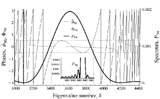
(a)

(b)

(c)

(d)

Figure 4: The maximally mixed state (13) in communication line of $N_{c}=5473$ nodes with $N_{S}=N_{R}=10$ at $t_{0}=5404.02$. (a) The spectrum $P_{Nk}$, the optimizing phases $\tilde{\phi}_{Nk}=\phi_{Nk}+\pi k$ and the resulting phases $\Phi_{Nk}=\phi_{Nk}-\lambda^{H}_{k}t_{0}$. The inset represent the spectrum $P_{Nk}$ over the whole spectral interval; (b) The amplitudes and the phases of the elements of the vector (21) (or the initial projections $f_{n}(0)=\langle n|\Pi_{S}^{+}U\Pi_{S}|1\rangle$); (c) The profile of the absolute values of the projections $|f_{n}(t_{0})|$; the inset: the amplitudes and the phases of the elements of the vector (22).

Condition (32) (the horizontal dotted lines in Fig.4a) selects the spectral interval $3405\leq k\leq 3886$ (the vertical dotted lines). Therefore, unlike the case of high-probability state creation, not all large-amplitude harmonics are involved in the state-creation process (see also the inset in Fig.4a).

Finally, we represent the amplitudes and phases of the elements of the column vector (21) and the row-vector (22), respectively, in Figs.4b and 4c (inset). Similar to Fig. 3b,c these figures confirm the symmetry (19). In Fig.4c we also show the profile of the absolute values of the projections $|f_{n}(t_{0})|$. Here, $f_{n}$, $n=N-N_{R}+1=5464,\dots,N-1=5472$ are identical to zero because of the unitary transformations $U$ and $V$ in formula (20).

IV Two-qubit state creation

In order to cover the large region of the two-qubit receivers state space we need to replace the one-excitation initial state (2) with the two-excitation one:

$$|\Psi_{0}\rangle=a_{0}|0\rangle+\sum_{i=1}^{N_{S}}a_{i}|i\rangle+\sum_{{i,j=1}\atop{j>i}}^{N_{S}}a_{ij}|ij\rangle,\;\;\sum_{i=0}^{N}|a_{i}|^{2}+\sum_{{i,j=1}\atop{j>i}}^{N_{S}}|a_{ij}|^{2}=1,$$ (33)

where $|ij\rangle$ is the state with the $i$th and $j$th spins excited. Now, instead of (6), the density matrix $\rho^{R}$ is given by the formula

$$\rho^{R}={\mbox{Tr}}_{1,\dots,N-2}|\Psi^{V}\rangle\langle\Psi^{V}|,\;\;|\Psi^{V}\rangle=e^{-iHt}|\Psi_{0}\rangle,$$ (34)

where trace is taken over all the nodes except the nodes of the receiver. Before proceeding to the state creation we need to determine the time instant $t_{0}$ for the state registration. We take the time instant maximizing the quantity

$$\varkappa=\langle N|\rho^{R}|N\rangle+\langle N-1|\rho^{R}|N-1\rangle+\langle N,N-1|\rho^{R}|N,N-1\rangle$$ (35)

averaged over the initial states (33),

$$\max_{t}\langle\varkappa\rangle=\langle\varkappa\rangle|_{t=t_{0}},$$ (36)

where $\langle\cdot\rangle$ means the average over pure initial states of the sender. The formula simplifying the calculation of $t_{0}$ is derived in Appendix, Sec. VI.1.

The creation of two-qubit states requires using the two-excitation dynamics and therefore this case becomes more complicated for numerical simulations. We restrict ourselves to the four-qubit sender ($N_{S}=4$) and two-qubit receiver without involving the extended receiver ($N_{R}=2$), and consider only the eigenvalue creation. The all possible values of three independent eigenvalues of the two-qubit state form a tetrahedron in the three-dimensional space of independent eigenvalues $\lambda_{i}$, $i=1,2,3$ (remember that $\lambda_{4}=1-\sum_{i=1}^{3}\lambda_{i}$) with the vertexes $L_{1}=(1,0,0)$, $L_{2}=\frac{1}{2}(1,1,0)$, $L_{3}=\frac{1}{3}(1,1,1)$ and $L_{4}=\frac{1}{4}(1,1,1)$, corresponding to the states, respectively, $\rho^{R}_{1}={\mbox{diag}}(1,0,0,0)$, $\rho^{R}_{2}=\frac{1}{2}{\mbox{diag}}(1,1,0,0)$, $\rho^{R}_{3}=\frac{1}{3}{\mbox{diag}}(1,1,1,0)$ and $\rho^{R}_{4}=\frac{1}{4}{\mbox{diag}}(1,1,1,1)$, as shown in Fig.5.

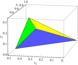
Figure 5: The three-dimensional region of the independent spectral parameters $\lambda_{i}$, $i=1,2,3$ of the two-qubit receiver’s state space is represented by the tetrahedron with the vertexes $L_{1}=(1,0,0)$, $L_{2}=\frac{1}{2}(1,1,0)$, $L_{3}=\frac{1}{3}(1,1,1)$ and $L_{4}=\frac{1}{4}(1,1,1)$. The whole tetrahedron can be created only in the short communication lines with $N\leq 16$.

Of course, not all points inside of this tetrahedron are achievable in long chains, so that each point $(\lambda_{1},\lambda_{2},\lambda_{3})$ has its own critical length $N_{c}(\lambda_{1},\lambda_{2},\lambda_{3})$ such that this point is not creatable in the communication line with $N>N_{c}$. For instance, the vertex $L_{1}$ is creatable in the communication line of any length, i.e. $N_{c}(L_{1})=\infty$. In addition, $N_{c}(L_{2})=191$ was calculated in Sec.III.2. The direct calculations (see Appendix, Sec. VI.2, for details) show that $N_{c}(L_{3})=N_{c}(L_{4})=16$. Thus, the whole tetrahedron can be created only in the short communication lines with $N\leq 16$.

To get some overview of critical lengths $N_{c}$ as a function of eigenvalues we calculate them for the lattice of points

$$\lambda_{1}\geq\lambda_{2}\geq\lambda_{3},\;\;\lambda_{i}=\frac{p_{i}}{12},\;\;p_{i}\in{\mathbb{Z}}$$ (37)

as shown in Fig.6. We can conclude that, with an increase in $N$, the creatable points are accumulating around the edge of the tetrahedron connecting the vertexes $L_{1}$ and $L_{2}$, see Fig.6a. Notice that calculating $N_{c}$ for the case $\lambda_{3}=\lambda_{4}=0$ shown in Fig.6a we use the one-excitation initial state and the optimization protocol based on the SVD (see Secs.II.1, III). The two-excitation initial state does not change the result, which is confirmed by the numerical simulations.

(a)

(b)

(c)

(d)

Figure 6: The critical length $N_{c}$ in dependence on the eigenvalues of the creatable state for the lattice of points (37). $N_{c}$ is indicated on the plane $(\lambda_{1},\lambda_{2})$ by the integer numbers, while $\lambda_{3}$ is given as a parameter in figures (a)-(d). Two critical lengths are missing. The first one corresponds to $\lambda_{3}=\frac{1}{3}$: $N_{c}(\frac{1}{3},\frac{1}{3},\frac{1}{3})=16$. The second critical length $N_{c}(1,0,0)=\infty$ must be at the right lower corner of figure (a). The critical length increases with approaching the line $\lambda_{3}=0$, $\lambda_{2}=1-\lambda_{1}$. The figure (a) is constructed using one-excitation initial state and the optimization protocol based on the SVD. The optimization in the case $\lambda_{3}>0$, figures (b)-(d), is performed using the approach of Sec.IV.

V Conclusion

In this paper we consider the optimization problem of the remote creation of quantum states . As the optimization tool we use the unitary transformations of the $N_{S}$-qubit sender and $N_{R}$-qubit extended receiver (which includes the receiver as a subsystem). For the one-qubit state, we consider the creation of two types of states: (i) (almost) pure state with single excitation of one-qubit receiver (this process is an analogue of the HPST) and (ii) the creation of maximally mixed state (the state with two equal eigenvalues). In both cases we investigate the dependence of the critical length on the dimensionality of the sender ($N_{S}$) and extended receiver ($N_{R}$) showing that $N_{c}$ grows with an increas in both $N_{S}$ and $N_{R}$. Thus, restricting ourselves to the 10-qubit sender and extended receiver we achieve $N_{c}=776$ for the high probability state creation and $N_{c}=5473$ for the creation of the maximally mixed state.

Considering the spectral representation of the state evolution we explicitly demonstrate that the optimal parameters of the sender’s initial state and of the unitary transformation of the extended receiver provide (i) the large spectral amplitudes and (ii) the proper spectral phases. Thus, almost the whole spectrum with large spectral amplitudes is involved into the high-probability state creation process (i.e., the spread of their phases satisfies condition (32)), whereas only half of them serve to create the maximally mixed state.

The creation of two-qubit states is more complicated because it is based on the two-excitation dynamics. Therefore we study only a particular example of communication line with four-qubit sender and two-qubit receiver (without the extended receiver) and consider the problem of eigenvalue creation. The creatable subregion form the tetrahedron in the three-dimensional space of the independent eigenvalues $\lambda_{i}$, $i=1,2,3$. We study the critical length $N_{c}$ as a function of a point inside of the above tetrahedron (i.e., the maximal length of the communication line allowing us to create a particular point inside of the tetrahedron). In particular, we have found $N_{c}(L_{1})=\infty$, $N_{c}(L_{2})=191$, $N_{c}(L_{3})=N_{c}(L_{4})=16$. Therefore, any point inside of the tetrahedron can be created using the communication line of $N\leq 16$ nodes.

This work is partially supported by the program of RAS ”Element base of quantum computers”(No. 0089-2015-0220) and by the Russian Foundation for Basic Research, grant No.15-07-07928.

VI Appendix

VI.1 Optimal time instant for state registration

We find the time instant maximizing the quantity $\varkappa$ (35) averaged over the initial states (33), see Eq.(36). By its definition (6), $\rho^{R}$ is a Hermitian form (the exact formula for $\rho^{R}$ is given in SZ_2016 ). Consequently, the quantity $\varkappa$ is a Hermitian form as well and can be written as

$$\varkappa(|\Psi_{0}\rangle)=\langle\Psi_{0}|\Pi_{S}^{+}A\Pi_{S}|\Psi_{0}\rangle,$$ (38)

where $A$ is a Hermitian operator independent on the parameters $a_{i}$ and $a_{ij}$. We can diagonalize $A$:

$$A={\mathcal{U}}\Omega{\mathcal{U}}^{+},$$ (39)

where $\Omega={\mbox{diag}}(\tilde{\lambda}_{1}\dots\tilde{\lambda}_{\tilde{N}_{S}})$ is the diagonal matrix of the eigenvalues and ${\mathcal{U}}$ is the corresponding matrix of the eigevectors of $A$. Here, $\tilde{N}_{S}=N_{S}(N_{S}+1)/2+1$ is the dimensionality of the basis of the sender’s state space, whose elements have the form (33). Obviously,

$$\langle\varkappa(\Psi_{0})\rangle=\big{\langle}\langle\Psi_{0}|\Pi_{S}^{+}A\Pi_{S}|\Psi_{0}\rangle\big{\rangle}=\big{\langle}\langle\Psi_{0}|\Pi_{S}^{+}\Omega\Pi_{S}|\Psi_{0}\rangle\big{\rangle}=$$

$$\sum_{j=1}^{\tilde{N}_{S}}\big{\langle}\langle\Psi_{0}|\Pi_{S}^{+}{\mbox{diag}}(\tilde{\lambda}_{j}\underbrace{0\dots 0}_{\tilde{N}_{S}-1})\Pi_{S}|\Psi_{0}\rangle\big{\rangle}=\frac{1}{\tilde{N}_{S}}\sum_{j=1}^{\tilde{N}_{S}}\big{\langle}\langle\Psi_{0}|\Pi_{S}^{+}{\mbox{diag}}(\underbrace{\tilde{\lambda}_{j}\dots\tilde{\lambda}_{j}}_{\tilde{N}_{S}})\Pi_{S}|\Psi_{0}\rangle\big{\rangle}=$$

$$\sum_{j=1}^{\tilde{N}_{S}}\frac{\tilde{\lambda}_{j}}{\tilde{N}_{S}}=\frac{{\mbox{Tr}}A}{\tilde{N}_{S}},$$

In turn,

$${\mbox{Tr}}A=\sum_{i=1}^{N_{S}}\langle i|\Pi_{S}^{+}A\Pi_{S}|i\rangle+\sum_{{i,j=1}\atop{j>i}}^{N_{S}}\langle ij|\Pi_{S}^{+}A\Pi_{S}|ij\rangle=\sum_{i=1}^{N_{S}}\varkappa(|i\rangle)+\sum_{{i,j=1}\atop{j>i}}^{N_{S}}\varkappa(|ij\rangle).$$ (41)

All in all, Eqs.(VI.1) and (41) yield

$$\langle\varkappa(\Psi_{0})\rangle=\frac{1}{\tilde{N}_{S}}\left(\sum_{i=1}^{N_{S}}\varkappa(|i\rangle)+\sum_{{i,j=1}\atop{j>i}}^{N_{S}}\varkappa(|ij\rangle)\right).$$ (42)

Consequently, we need to find the time instant $t_{0}$ maximizing the rhs of Eq.(42). Thus the multi-parameter optimization is reduced to the optimization over the single parameter $t$.

VI.2 Eigenvalue creation in two-qubit receiver

The parameters $a_{i}$ and $a_{ij}$ in the initial state (33) which result to the states with four and three equal eigenvalues (the vertex $L_{3}$ and $L_{4}$ of the tetrahedron in Fig.5) can be found using the characteristic equation

$$|\rho^{R}-\lambda I|=\lambda^{4}-\lambda^{3}+A\lambda^{2}+B\lambda+C,\;\;\;C=\det\rho^{R},$$ (43)

where $A$, $B$ and $C$ are functions of the parameters $a=(a_{i}:i=1,\dots,N,a_{ij}:,j>i,i=1,\dots,N-1,\;j=2,\dots,N)$ and time $t$. In general, if we are interested in a state with the fixed set of eigenvalues $\lambda_{i}$, $i=1,2,3$, then the coefficients of the characteristic equation are the known functions $A_{0}$, $B_{0}$ and $C_{0}$ of $\lambda_{i}$, and we have to find the set of parameters $a$ solving the following system at the optimized time instant $t_{0}$ (found in Appendix, Sec.VI.1):

$$A(a,t_{0})=A_{0}(\lambda_{1},\lambda_{2},\lambda_{3}),\;\;B(a,t_{0})=B_{0}(\lambda_{1},\lambda_{2},\lambda_{3}),\;\;C(a,t_{0})=C_{0}(\lambda_{1},\lambda_{2},\lambda_{3}).$$ (44)

To find the approximate solution to this system we minimize the discrepancy

$$\varepsilon(\lambda_{1},\lambda_{2},\lambda_{3})=\sqrt{\left(A-A_{0}\right)^{2}+\left(B-B_{0}\right)^{2}+\left(C-C_{0}\right)^{2}}.$$ (45)

If the minimized values of $\varepsilon$ exceeds the certain value for some $N$, then we say that the state is not creatable in the communication line of length $N$.

To clarify the above arguments, we consider the creation of the vertexes $L_{3}$ and $L_{4}$ of the tetrahedron in Fig.5. For them we have, respectively, $A_{0}(\frac{1}{3},\frac{1}{3},\frac{1}{3})=\frac{1}{3}$, $B_{0}(\frac{1}{3},\frac{1}{3},\frac{1}{3})=-\frac{1}{27}$, $C_{0}(\frac{1}{3},\frac{1}{3},\frac{1}{3})=0$ and $A_{0}(\frac{1}{4},\frac{1}{4},\frac{1}{4})=\frac{3}{8}$, $B_{0}(\frac{1}{4},\frac{1}{4},\frac{1}{4})=-\frac{1}{16}$, $C_{0}(\frac{1}{4},\frac{1}{4},\frac{1}{4})=\frac{1}{256}$. The accuracies $\varepsilon(L_{3})$ and $\varepsilon(L_{4})$ as functions of $N$ are shown in Fig.7. Passing from $N=16$ to $N=17$, both $\varepsilon(L_{3})$ and $\varepsilon(L_{4})$ jump, respectively, from $\sim 10^{-12}$ to $\sim 10^{-5}$ and from $\sim 10^{-13}$ to $\sim 10^{-4}$. This indicates that the vertexes $L_{3}$ and $L_{4}$ are not achievable for $N>16$. Therefore we conclude that $N_{c}(L_{4})=N_{c}(L_{3})=16$.

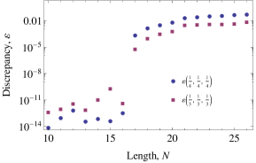
Figure 7: The accuracies $\varepsilon(L_{3})$ and $\varepsilon(L_{4})$ as functions of the length of communication line.

References

• (1) S. Bose, Phys. Rev. Lett. 91, 207901 (2003)
• (2) M.Christandl, N.Datta, A.Ekert and A.J.Landahl, Phys.Rev.Lett. 92, 187902 (2004)
• (3) C.Albanese, M.Christandl, N.Datta and A.Ekert, Phys.Rev.Lett. 93, 230502 (2004)
• (4) P.Karbach and J.Stolze, Phys.Rev.A 72, 030301(R) (2005)
• (5) G.Gualdi, V.Kostak, I.Marzoli and P.Tombesi, Phys.Rev. A 78, 022325 (2008)
• (6) A.Wójcik, T.Luczak, P.Kurzyński, A.Grudka, T.Gdala, and M.Bednarska, Phys. Rev. A 72, 034303 (2005)
• (7) L. Banchi, T. J. G. Apollaro, A. Cuccoli, R. Vaia, and P. Verrucchi, Phys.Rev.A 82, 052321 (2010)
• (8) A. Zwick, O. Osenda, J. Phys. A Math. Theor., 44, 105302 (2011)
• (9) L. Banchi, T. J. G. Apollaro, A. Cuccoli, R. Vaia and P. Verrucchi, New J. Phys. 13, 123006 (2011)
• (10) T. J. G. Apollaro, L. Banchi, A. Cuccoli, R. Vaia, P. Verrucchi, Phys. Rev. A 85, 052319 (2012)
• (11) S.I.Doronin, A.I.Zenchuk, Phys. Rev. A 81, 022321 (2010)
• (12) Henry L. Haselgrove, Phys. Rev. A 72, 062326 (2005)
• (13) C. Allen Bishop, Yong-Cheng Ou, Zhao-Ming Wang, Mark S. Byrd, Phys. Rev. A 81, 042313 (2010)
• (14) G. A. Bochkin and A. I. Zenchuk, Phys.Rev.A 91, 062326(11) (2015)
• (15) E.I.Kuznetsova and A.I.Zenchuk, Phys.Lett.A 372, pp.6134-6140 (2008)
• (16) J.Stolze, G. A. Álvarez, O. Osenda, A. Zwick in Quantum State Transfer and Network Engineering. Quantum Science and Technology, ed. by G.M.Nikolopoulos and I.Jex, Springer Berlin Heidelberg, Berlin, p.149 (2014)
• (17) A. Bayat and V. Karimipour, Phys.Rev.A 71, 042330 (2005)
• (18) P. Cappellaro, Phys.Rev.A 83, 032304 (2011)
• (19) W. Qin, Ch. Wang, G. L. Long, Phys.Rev.A 87, 012339 (2013)
• (20) A.Bayat, Phys. Rev. A 89, 062302 (2014)
• (21) C. Godsil, S. Kirkland, S. Severini, Ja. Smith, Phys. Rev. Lett. 109, 050502 (2012)
• (22) R.Sousa, Ya. Omar, New J. Phys. 16, 123003 (2014).
• (23) D. Burgarth and S. Bose, Phys.Rev.A 71, 052315 (2005)
• (24) K. Shizume, K. Jacobs, D. Burgarth, and S. Bose, Phys. Rev. A 75, 062328 (2007)
• (25) G.A.Bochkin, A.I.Zenchuk, Qunt. Inf. Comp., 16, No. 15-16, 1349 (2016)
• (26) J.Stolze and A.I.Zenchuk, Quantum Inf. Process 15, 3347 (2016)