Long period variable stars in NGC 147 and NGC 185. I. Their star formation histories

Abstract

NGC 147 and NGC 185 are two of the most massive satellites of the Andromeda galaxy (M 31). Close together in the sky, of similar mass and morphological type dE, they possess different amounts of interstellar gas and tidal distortion. The question therefore is, how do their histories compare? Here we present the first reconstruction of the star formation histories of NGC 147 and NGC 185 using long-period variable stars. These represent the final phase of evolution of low- and intermediate-mass stars at the asymptotic giant branch, when their luminosity is related to their birth mass. Combining near-infrared photometry with stellar evolution models, we construct the mass function and hence the star formation history. For NGC 185 we found that the main epoch of star formation occurred 8.3 Gyr ago, followed by a much lower, but relatively constant star formation rate. In the case of NGC 147, the star formation rate peaked only 7 Gyr ago, staying intense until $\sim 3$ Gyr ago, but no star formation has occurred for at least 300 Myr. Despite their similar masses, NGC 147 has evolved more slowly than NGC 185 initially, but more dramatically in more recent times. This is corroborated by the strong tidal distortions of NGC 147 and the presence of gas in the centre of NGC 185.

1 Introduction

Dwarf galaxies are the most abundant type of galaxies in the universe, spanning a huge range in stellar mass, luminosity and surface brightness. They come in two main flavours: dwarf Irregulars (dIrrs) and dwarf Spheroidal/Ellipticals (dSph/dEs). These are distinguished principally by the significant interstellar medium (ISM) in dIrrs and almost complete lack thereof in dSphs/dEs, but their star formation histories also differ, with dIrrs being “younger” (Battinelli & Demers 2006). Most dSph/dEs are located in the dense inner regions of galaxy groups and clusters, close to massive spiral or elliptical galaxies. On the other hand, dIrrs are often more isolated. This strongly suggests that environmental effects transform dIrrs into dSph/dEs.

The Star Formation History (SFH) is one of the most important tracers of the evolution of galaxies. We have developed a novel method to use Long-Period Variable stars (LPVs) to reconstruct the SFH, which we have successfully applied the Local Group galaxies M 33 (Javadi, van Loon & Mirtorabi 2011; Javadi et al. 2016) and the Magellanic Clouds (Rezaeikh et al. 2014). The most evolved stars with low to intermediate mass, at the tip of the Asymptotic Giant Branch (AGB) show brightness variations on timescales of $\approx 100$ to $>1000$ days due to radial pulsation. LPVs represent the most luminous phase in their evolution, $\sim 3000$–60,000 L_⊙, and reach their maximum brightness at near-infrared wavelengths. Intermediate-mass AGB stars may become carbon stars as a result of the dredge up of carbon synthesized in the helium thermal pulses; the resulting change in opacity reddens their colours. Since the maximum luminosity attained on the AGB relates to the star’s birth mass, we can use the brightness distribution function of LPVs to construct the birth mass function and hence the Star Formation Rate (SFR) as a function of time. In this paper we present the results from application of this method to the Local Group dEs NGC 147 and NGC 185.

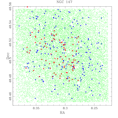
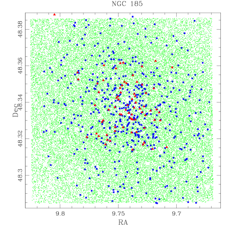
Figure 1: Spatial distribution of AGB stars (green dots; Nowotny et al. 2003), LPVs (blue squares; Lorenz et al. 2011) and carbon stars (red triangles; Sohn et al. 2006; Kang et al. 2005) across NGC 147 (left) and NGC 185 (right).

NGC 147 and NGC 185 were selected for the availability of suitable data of a significant number of LPVs (Lorenz et al. 2011), but also in their own right. Both are satellites of Andromeda (M 31), the most massive member of the Local Group. NGC 147 and NGC 185 share fundamental properties such as luminosity ($M_{\rm V}\sim 16$; Crnojević et al. 2014) and velocity dispersion (25 km s^-1; Geha et al. 2010), but they differ in many other aspects. NGC 185 contains some gas, dust and shows evidence for recent star formation in its central regions, while NGC 147 is destitute of gas and dust and shows no sign of recent star formation activity (Young & Lo 1997; Welch, Sage & Mitchell 1998; Marleau, Noriega-Crespo & Misselt 2010; De Looze et al. 2016). The mean metallicity of NGC 147 based on photometry of the red giant branch is [M/H]${}_{\rm NGC\,147}\approx-1.1$ to $-1$, which is slightly higher than that of NGC 185, [M/H]${}_{\rm NGC\,185}\approx-1.3$ to $-1.1$ (Davidge 1994; McConnachie et al. 2005; Geha et al. 2010). Spectroscopic measurements indicate the presence of a more metal-rich population, with [M/H]${}_{\rm NGC\,147}=-0.5\pm 0.1$ and [M/H]${}_{\rm NGC\,185}=-0.9\pm 0.1$ (Vargas, Geha & Tollerud 2014). The latter displays a metallicity gradient (Vargas et al. 2014; Crnojević et al. 2014), reaching [M/H]${}_{\rm NGC\,185}\sim-2$ at the edge (Ho et al. 2015). NGC 147 and NGC 185 are very close in projection on the sky ($58^{\prime}$), leading some to argue that they may be a bound galaxy pair (van den Bergh 1998). However, kinematic evidence suggests that they may not be gravitationally bound (Geha et al. 2010; Watkins, Evans & van de Ven 2013). NGC 147 is tidally distorted, whereas NGC 185 is not (Ferguson & Mackey 2016). Their distances have been estimated (McConnachie et al. 2005) at $d_{\rm NGC147}=675\pm 27$ kpc (distance modulus $\mu_{\rm NGC147}=24.15$ mag) and $d_{\rm NGC185}=616\pm 26$ kpc ($\mu_{\rm NGC185}=23.95$ mag).

In this paper we construct the birth mass function of LPVs and derive the SFH in the inner $6\hbox to0.0pt{.\hss}^{\prime}5\times 6\hbox to0.0pt{.\hss}^{\prime}5$ regions of NGC 147 and NGC 185. In section 2 we introduce the photometric catalogues. Section 3 explains our method. In section 4 we present the results. Finally, a discussion and conclusions follow in sections 5 and 6. In an Appendix, we provide additional results for different assumptions regarding the metallicity.

2 Data

We take advantage of a number of published photometric catalogues (see below). The dimensions of NGC 147 and NGC 185 are $13\hbox to0.0pt{.\hss}^{\prime}2\times 7\hbox to0.0pt{.\hss}^{\prime}8$ and $11\hbox to0.0pt{.\hss}^{\prime}7\times 10\hbox to0.0pt{.\hss}^{\prime}0$ , however the data only cover the central $6\hbox to0.0pt{.\hss}^{\prime}5\times 6\hbox to0.0pt{.\hss}^{\prime}5$ regions (see Fig. 1 – one thing that is immediately apparent is that the AGB stars in NGC 147 are much less centrally concentrated than in NGC 185).

2.1 The optical data

As part of a photometric survey of Local Group galaxies to resolve AGB stars, Nowotny et al. (2003) obtained images of NGC 147 and NGC 185 in four optical filters, viz. the broad-band visual $V$ and near-infrared Gunn $i$ and filters centred on the TiO and CN molecular bands, respectively, using the Nordic Optical Telescope (NOT) in the year 2000. They used the ALFOSC instrument, with a pixel size of $0\hbox to0.0pt{.\hss}^{\prime\prime}189$ pixel^-1 yielding a $6\hbox to0.0pt{.\hss}^{\prime}5\times 6\hbox to0.0pt{.\hss}^{\prime}5$ field of view (FoV). Although this will include the majority of the stars, our survey is not totally complete in terms of area. Figure 1 shows the observed areas, corresponding to physical sizes of $1.27\times 1.27$ kpc² on NGC 147 and $1.16\times 1.16$ kpc² on NGC 185. A total of 18 300 and 26 496 AGB stars were detected within these regions in NGC 147 and NGC 185, respectively (green dots in figure 1).

2.2 The near-infrared data

2.2.1 LPVs

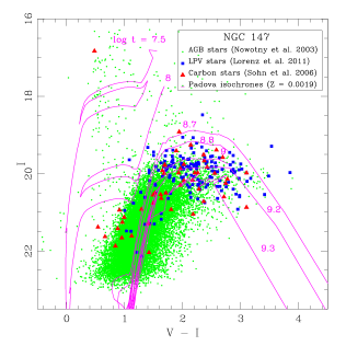
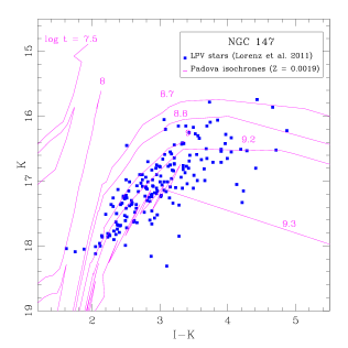
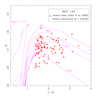
Figure 2: CMDs of NGC 147. Isochrones from Marigo et al. (2008) are labelled with logarithmic ages.

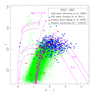
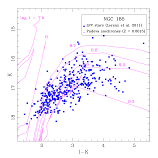
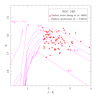
Figure 3: CMDs of NGC 185. Isochrones from Marigo et al. (2008) are labelled with logarithmic ages.

For our method to derive the SFH, we need to identify the LPVs among the AGB stars. For this we have used the catalogue of LPVs from Lorenz et al. (2011). Like Nowotny et al. (2003), they observed NGC 147 and NGC 185 with ALFOSC on the NOT, using the Gunn $i$ band, on 38 nights between October 2003 and February 2006. They also observed NGC 147 and NGC 185 once in the $K$ band, using NOTCam (on the NOT) in September 2004. NOTcam yields a field-of-view of $4^{\prime}\times 4^{\prime}$; to cover the ALFOSC field-of-view they created a mosaic of four overlapping images with NOTcam. The LPVs were identified by means of the image subtraction technique. The resulting catalogue contains 213 LPVs in the direction of NGC 147 and 513 LPVs in the direction of NGC 185. The loci of the LPVs are depicted in figure 1 with blue squares. As can be seen in figure 1, the central region of NGC 185 is denser towards the centre. Hence, the identification of variable stars in the central regions is incomplete because of crowding.

2.2.2 Carbon stars

We have also made use of the catalogues of carbon stars published in Sohn et al. (2006) and Kang et al. (2005). They obtained near-infrared images with the Canada–France–Hawai’i Telescope in June 2004, using the CFHTIR imager and $J$, $H$ and $K^{\prime}$ filters, each field covering $3\hbox to0.0pt{.\hss}^{\prime}6\times 3\hbox to0.0pt{.\hss}^{\prime}6$. Sohn et al. (2006) present the photometry of 91 carbon stars in NGC 147, and Kang et al. (2005) present the photometry of 73 carbon stars in NGC 185. The loci of the carbon stars are depicted in figure 1 with red triangles.

2.3 Colour–magnitude diagrams

The $K$-band photometry is the best suited for calculating the SFR, because the spectral energy distributions of stars near the tip of the AGB peak at near-infrared wavelengths, minimising uncertainties in bolometric corrections, and interstellar and circumstellar extinction is much less important than at optical wavelengths. Because carbon stars can be used to trace (part of) the AGB, we have cross matched the LPV and carbon star catalogues, using the average of $K$-band magnitudes for stars in common. We can thus examine the location of the AGB stars in a colour–magnitude diagram (CMD), in comparison with isochrones from the stellar evolution models from the Padova group (Marigo et al. 2008) that we use later in our technique to derive the SFH. The CMDs of NGC 47 and NGC 185 are presented in figures 2 and 3, respectively.

The optical CMDs (left panels of figures 2 and 3) clearly show the densely populated AGB, from $(V-I)\sim 1$ to $\sim 2$ mag. The smaller number of brighter/bluer stars are likely Galactic foreground dwarfs. The carbon stars occupy the bright/red portion of the AGB as these are in advanced stages of AGB evolution; likewise, the LPVs occupy the region where the AGB terminates, thus validating our premise that LPVs can be used to determine the luminosity at the tip of the AGB.

Padova isochrones (Marigo et al. 2008) are consistent with the photometry with the adopted distance moduli and metallicities of $Z=0.0019$ for NGC 147 and $Z=0.0015$ for NGC 185. They include the effects of circumstellar dust formed in the winds from the most evolved AGB stars, at $(V-I)\,\vbox{\hbox{$>$}\offinterlineskip\hbox{$\sim$}}\,2.5$ mag.

Our method, which is explained in section 3, Javadi et al. (2011, 2016) and Rezaeikh et al. (2014), is based on the luminosity peak of LPVs in the $K$ band. Figures 2 and 3 show the location of the LPVs in the near-infrared CMDs (middle panels), as well as the carbon stars for comparison (right panels). Clearly, the vast majority of LPVs are several Gyr old ($\log t>9$), with the youngest $\sim 400$–500 Myr old ($\log t=8.6$–8.7).

3 Method: star formation history

The SFH of a galaxy is a measure of the rate at which gas mass was converted into stars over a time interval in the past. Or in other words, it is the SFR, $\xi$ (in M_⊙ yr^-1), as a function of time. The amount of stellar mass, $dM$, created during a time interval, $dt$, is:

$$dM(t)=\xi(t)\ dt.$$ (1)

The number of formed stars are related to the total mass by the following equation:

$$dN(t)=\frac{\int_{\rm min}^{\rm max}f_{\rm IMF}(m)\ dm}{\int_{\rm min}^{\rm max}f_{\rm IMF}(m)m\ dm}\ dM(t),$$ (2)

where $f_{\rm IMF}$ is the Initial Mass Function (IMF). We use the IMF defined in Kroupa (2001):

$$f_{\rm IMF}=Am^{-\alpha},$$ (3)

where $A$ is the normalization constant and $\alpha$ is defined depending on the mass range:

$$\alpha=\left\{\begin{array}[]{cclcl}+0.3\pm 0.7&{\rm for}&{\rm min}&<\frac{m}{{\rm M}_{\odot}}<&0.08\\ +1.3\pm 0.5&{\rm for}&0.08&<\frac{m}{{\rm M}_{\odot}}<&0.5\\ +2.3\pm 0.3&{\rm for}&0.5&<\frac{m}{{\rm M}_{\odot}}<&{\rm max}\\ \end{array}\right.$$ (4)

The minimum and maximum mass were assumed to be 0.02 and 200 M_⊙, respectively.

We need to relate this to the number of stars, $N$, which are variable at the present time. If stars with mass between $m(t)$ and $m(t+dt)$ are LPVs at the present time, then the number of LPVs created between times $t$ and $t+dt$ is

$$dn(t)=\frac{\int_{m(t)}^{m(t+dt)}f_{\rm IMF}(m)\ dm}{\int_{\rm min}^{\rm max}f_{\rm IMF}(m)\ dm}\ dN(t).$$ (5)

Substituting equation 1 and 2 in equation 5 gives

$$dn(t)=\frac{\int_{m(t)}^{m(t+dt)}f_{\rm IMF}(m)\ dm}{\int_{\rm min}^{\rm max}f_{\rm IMF}(m)m\ dm}\ \xi(t)\ dt.$$ (6)

We are considering an age bin of $dt$, to determine $\xi(t)$. The number of LPVs observed in this age bin, $dn^{\prime}$, depends on the duration of the evolutionary stage during which the variability occurs:

$$dn^{\prime}(t)=\frac{\delta t}{dt}\ dn(t).$$ (7)

Finally, by combining the above equations we obtain a relation to calculate the SFR based on LPV counts:

$$\xi(t)=\frac{\int_{\rm min}^{\rm max}f_{\rm IMF}(m)m\ dm}{\int_{m(t)}^{m(t+dt)}f_{\rm IMF}(m)\ dm}\ \frac{dn^{\prime}(t)}{\delta t}.$$ (8)

To obtain the SFR we need to determine the individual stars’ masses, ages ($t$) and durations of pulsation ($\delta t$). For this we rely on theoretical models. The most appropriate theoretical models for our purpose are the Padova models (Marigo et al. 2008), for the following reasons:
$\bullet$ They have prepared models for the required range in birth mass ($0.8<M<30$ M_⊙) by combining models for intermediate-mass stars ($M<7$ M_⊙) with those for more massive stars ($M>7$ M_⊙; Bertelli et al. 1994)) and corrections for low-mass, low-metallicity AGB tracks (Girardi et al. 2010);
$\bullet$ They are based on computations carried out through the entire thermal pulsing AGB until they enter the post-AGB phase, in a manner that is consistent with the computation of the preceding evolutionary stages. The models account for the third dredge-up mixing of the stellar envelope as a result of the helium-burning pulses, and the increased luminosity of massive AGB stars undergoing hot bottom burning (Iben & Renzini 1983);
$\bullet$ The models account for the molecular opacity in the cool atmospheres of red giants, including changes as a result of the transformation from oxygen-dominated M-type AGB stars to carbon stars in the approximate birth-mass range of $M\sim 1.5$–4 M_⊙ (Girardi & Marigo 2007);
$\bullet$ They include predictions for dust production in the winds of LPVs and the associated attenuation and reddening of the synthetic photometry;
$\bullet$ They include predictions for the radial pulsation;
$\bullet$ They have been carefully transformed to various optical and infrared photometric systems;
$\bullet$ They are available via a user-friendly internet interface.
One shortcoming is that these models do not account for the final part of the evolution of super-AGB stars, i.e. stars in the mass range $0.7<\log M/{\rm M}_{\odot}<1.2$–1.3.

We note that the PARSEC+COLIBRI models are the latest Padova models and we use the Padova models that incorporate the relevant physics already. However, according to Marigo et al. (2013), the difference between the effective temperatures predicted by the two sets of models is negligible, and the same is true for the temperature at the base of the convective envelope. In the same paper they also show that their new models reproduce perfectly the core-mass luminosity relation adopted in the previous models, as well as confirming the predictions from alternative models (from Karakas et al. 2002). Taken together, this means that the observational properties do not change markedly between these models, and that the relationship between empirical quantities and theoretical parameters remains essentially unchanged and robust.

LPVs have reached the maximum luminosity on the AGB. On that premise, we have constructed a mass–$K$-band magnitude relation for the metallicity and distance modulus of NGC 147 ($Z=0.0019$ and $\mu=24.15$ mag; left panel of figure 4). All the figures and tables related to NGC 185 and to other metallicities used in this paper are presented in the Appendix.

There is an obvious excursion towards fainter $K$-band magnitudes for super-AGB stars, because their evolution to brighter $K$-band magnitudes has been omitted from the models. We thus interpolate over that range in mass (see Javadi et al. 2011); however, since we do not have any super-AGB stars in any of these dwarfs, we effectively only use the part of the Mass-Luminosity (ML) relation that is modelled carefully. In other words, the brightest stars have $K>15$ mag so we are in the regime of stars for which the models give reliable predictions. The coefficients of the piecewise linear relations between $K$-band magnitude and mass are listed in Table 1.

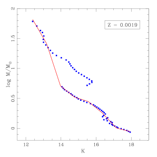
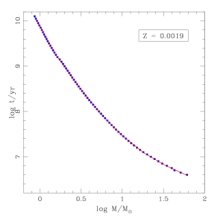
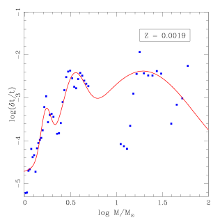
Figure 4: The dots refer to models from Marigo et al. (2008); (Left:) Mass–luminosity relation (in the $K$ band) for $Z=0.0019$ and a distance modulus of $\mu_{\rm NGC147}=24.15$ mag. The solid lines are linear spline fits, in which the function is interpolated over the super-AGB phase to massive red supergiants. (Middle:) Same, for the mass–age relation. (Right:) Same, for the mass–pulsation duration relation. The points show the ratio of pulsation duration to age, versus mass; the solid lines are multiple-Gaussian fits, interpolated over the super-AGB regime.

Table 1: Relation between birth mass and $K$-band magnitude, $\log M=aK+b$, for a distance modulus of $\mu_{\rm NGC147}=24.15$ mag.

$Z=0.0019$
$a$	$b$	validity range
$-0.508\pm 0.052$	$8.116\pm 0.676$	$K\leq 13.182$
$-0.893\pm 0.048$	1$3.185\pm 0.649$	$13.182<K\leq 13.975$
$-0.234\pm 0.048$	$3.974\pm 0.688$	$13.975<K\leq 14.767$
$-0.095\pm 0.044$	$1.931\pm 0.673$	$14.767<K\leq 15.560$
$-0.238\pm 0.038$	$4.151\pm 0.606$	$15.560<K\leq 16.352$
$-0.317\pm 0.032$	$5.437\pm 0.534$	$16.352<K\leq 17.145$
$-0.076\pm 0.042$	$1.311\pm 0.471$	$K>17.145$

We apply the following extinction corrections to dusty LPVs according to the isochrones in the middle panels of figures 2 and 3:

$$K_{\rm cor}=K+a_{\rm LPV}[(I-K)-(I-K)_{0}],$$ (9)

and to carbon stars according to the isochrones in the right panels of figures 2 and 3:

$$K_{\rm cor}=K+a_{\rm carbon}[(J-K)-(J-K)_{0}],$$ (10)

where $a_{\rm LPV}=0.24$ and $a_{\rm carbon}=0.59$ are the average slopes of the tracks for these two types of stars in their respective CMDs, and $(I-K)_{0}=2.6$ mag and $(J-K)_{0}=1.4$ mag are their mean colours at the point at which their tracks bend towards lower luminosity and redder colour.

The mass–age relation is shown in the middle panel of figure 4. This relates the birth mass of an LPV observed at the present time, to the time elapsed since its birth. The coefficients of this relation are listed in table 2, for the metallicity adopted for NGC 147.

Table 2: Relation between age and birth mass, $\log t=a\log M+b$.

$Z=0.0019$
$a$	$b$	validity range
$-3.221\pm 0.030$	$9.874\pm 0.002$	$\log{M}\leq 0.200$
$-2.511\pm 0.027$	$9.732\pm 0.009$	$0.200<\log{M}\leq 0.465$
$-2.278\pm 0.029$	$9.624\pm 0.018$	$0.465<\log{M}\leq 0.729$
$-1.856\pm 0.032$	$9.317\pm 0.028$	$0.729<\log{M}\leq 0.993$
$-1.442\pm 0.037$	$8.906\pm 0.041$	$0.993<\log{M}\leq 1.257$
$-1.062\pm 0.043$	$8.428\pm 0.059$	$1.257<\log{M}\leq 1.522$
$-0.833\pm 0.053$	$8.078\pm 0.087$	$\log{M}>1.522$

Massive stars spend less time in the LPV phase than lower mass stars, but a larger fraction of their entire lifetime (right panel of figure 4). The theoretical models were parameterised by a set of three Gaussian functions (table 3, for the metallicity adopted for NGC 147).

Table 3: Relation between the relative pulsation duration and birth mass, $\log(\delta t/t)=D+\Sigma_{i=1}^{3}a_{i}\exp\left[-(\log M[{\rm M}_{\odot}]-b_{i})^{2}/2c_{i}^{2}\right]$.

$Z=0.0019$
$D$	$i$	$a$	$b$	$c$
$-4.9$	1	1.02	0.23	0.056
	2	1.43	0.53	0.129
	3	2.52	1.29	0.576

To obtain the SFH, the following procedure was applied to each individual star:
$\bullet$ De-redden the $K$-band magnitude;
$\bullet$ Use table 1 to determine the birth mass;
$\bullet$ Use table 2 to determine the age of the star;
$\bullet$ Use table 3 to calculate the pulsation duration;
$\bullet$ As the number of young, massive LPVs is much smaller than the number of old, low-mass LPVs, to obtain uniform uncertainties in the SFR values we choose the age bin size such that they have equal numbers of stars. The error on the SFR in each bin is calculated using the following relation: $errorSFR[i]=\sqrt{n[i]}\times SFR[i]/n[i]$ where n is the number of stars in each bin i.

4 Results: star formation histories

Using the photometric catalogues of LPVs and carbon stars (section 2) and applying the method explained in detail in section 3, we estimate the SFRs in NGC 147 and NGC 185 during the broad time interval from 300 Myr to 13 Gyr ago.

4.1 Assuming constant metallicity over time

The SFR as a function of look-back time (age) in NGC 147 and NGC 185 is shown in figure 5. The horizontal bars represent the age bins.

Figure 5: SFHs in the central $6\hbox to0.0pt{.\hss}^{\prime}5\times 6\hbox to0.0pt{.\hss}^{\prime}5$ regions of NGC 147 (left) and NGC 185 (right), from LPV counts assuming a constant metallicity.

A peak of star formation occurred in NGC 147 at 7 Gyr ago ($\log t=9.85$; left panel in figure 5), when the SFR reached a level of $0.022\pm 0.004$ M_⊙ yr^-1 on average over an interval of $\sim 1.3$ Gyr. The SFR then dropped to $\sim 0.01$ M_⊙ yr^-1 between 4–6 Gyr ago. After a slight increase in SFR to $\sim 0.014$ M_⊙ yr^-1 it continues with 0.003–0.005 M_⊙ yr^-1. Of the total stellar mass in NGC 147 ($1.16\times 10^{8}$ M_⊙), 51% was formed during the period of intense star formation from 11 to 6.5 Gyr ago.

In NGC 185 (right panel in figure 5), the SFR shows an abrupt and brief enhancement 8.3 Gyr ago, reaching $0.062\pm 0.009$ M_⊙ yr^-1. After this, the SFR dropped precipitously; by 200 Myr ago it continued at a rate of 0.006–0.008 M_⊙ yr^-1. Of the total stellar mass in NGC 185 ($2.42\times 10^{8}$ M_⊙), 54% was formed between 10.2 and 7.6 Gyr ago. This is a similar fraction to that in NGC 147 but formed in roughly half the time.

4.2 Assuming different metallicities for the old and young stellar populations

As a galaxy ages, the metallicity of the ISM – and hence that of new generations of stars – changes as a result of nucleosynthesis and feedback from dying stars. So we expect older stars to have formed in more metal poor environments than younger stars have. To examine the effect of chemical evolution on the SFH we derive, we also considered the case in which the metallicity is lower than that assumed in section 4.1 for older stars and higher for younger stars.

Reported metallicities span the broad range of $0.0012<Z<0.0076$ for NGC 147 and $0.0008<Z<0.0030$ for NGC 185. We here adopt $Z=0.0015$ for $\log t\geq 9.2$ and $Z=0.0024$ for $\log t<9.2$, in NGC 147 (as opposed to a constant $Z=0.0019$), and $Z=0.0012$ and $Z=0.0019$ for these age groups in NGC 185 (cf. $Z=0.0015$). Figure 6 shows the resulting SFHs.

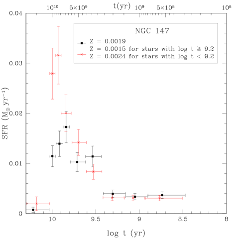
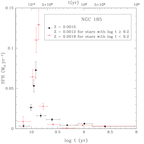
Figure 6: The effect on the SFH of a time-varying metallicity. (Left:) NGC 147 with a constant $Z=0.0019$ (black squares), or $Z=0.0015$ for $\log t\geq 9.2$ and $Z=0.0024$ for $\log t<9.2$ (red crosses); (Right:) NGC 185 with a constant $Z=0.0015$ (black squares), or $Z=0.0012$ for $\log t\geq 9.2$ and $Z=0.0019$ for $\log t<9.2$ (red crosses).

Two effects are obvious. Firstly, the star formation peak becomes almost twice as high, while more recent star formation is diminished. Secondly, the peak of star formation shifts in age. Curiously, it shifts towards older ages in NGC 147 but towards more recent times in NGC 185. The total stellar masses obtained from integration of the SFH also become larger: $1.81\times 10^{8}$ M_⊙ in NGC 147 and $4.70\times 10^{8}$ M_⊙ in NGC 185.

4.3 Overall effect of metallicity

We here expand on the analysis of the effects on the SFH resulting from the assumptions regarding the metallicity. The graphs and tables with the model relations can be found in the appendix. In figure 7 we plot the results from a wider range of assumed (constant) metallicity. Depending on the time in the history of the galaxy at which such metallicity may have been the norm, one could selectively read off the SFR accordingly.

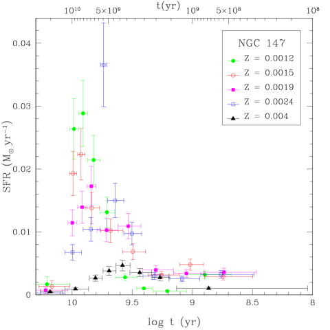
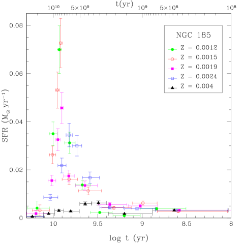
Figure 7: SFHs for different (constant) metallicity, for NGC 147 (left) and NGC 185 (right).

We confirm that the peak of star formation would shift towards older ages for lower metallicity. The effect is especially strong at the highest metallicity we consider here, $Z=0.004$ (which is typical of the ISM within the Small Magellanic Cloud). Such high metallicities are not expected to be reached within either NGC 147 or NGC 185, except perhaps for the youngest stars in NGC 147. We do not expect to see the dramatic drop in SFR at old ages as a result of such high metallicity. So our results do not change qualitatively when changing the assumed metallicity.

Table 4: Total stellar mass for different (constant) metallicity.

$Z$	$M_{\rm NGC\,147}$ (M⊙)	$M_{\rm NGC\,185}$ (M⊙)
$0.0012$	$1.67\times 10^{8}$	$3.40\times 10^{8}$
$0.0015$	$1.29\times 10^{8}$	$2.42\times 10^{8}$
$0.0019$	$1.16\times 10^{8}$	$2.03\times 10^{8}$
$0.0024$	$1.17\times 10^{8}$	$2.14\times 10^{8}$
$0.004$	$2.97\times 10^{7}$	$5.05\times 10^{7}$

Figure 8: SFHs in NGC 147 (left) and NGC 185 (right) in bins at galactocentric radii increasing from left to right and top to bottom.

The total stellar mass does depend on metallicity (see table 4); as the metallicity increases the total stellar mass decreases. However, this change is very small, $\vbox{\hbox{$<$}\offinterlineskip\hbox{$\sim$}}\,10$%, in the range $Z=0.0015$–0.0024.

4.4 Galactocentric radial gradients of the SFHs

Besides the history of the SFR, variations across the galaxy can elucidate on the mechanisms that governed the formation and evolution of the galaxy over cosmological times. The suggestion of a metallicity gradient in NGC 185 is one such example; here we explore whether the SFH has varied with location within the galaxy, specifically whether there is a galactocentric radial gradient. The results are presented in figure 8.

Roughly speaking, the peak in SFR diminishes by a factor $\sim 5$ between the innermost and outermost regions ($r\sim 0.6$ kpc). Note that the tidal tails of NGC 147 extend $\sim 2^{\circ}$ to either side, i.e. well beyond the region we probe here. The most striking variation in SFH that we see is in NGC 185, where recent star formation ($t<$ Gyr or $\log t<9$) is very prominent in the inner 0.1 kpc but completely lacking beyond 0.5 kpc. This may be related to the strong central concentration we noted in figure 1. NGC 147 exhibits a more uniform SFH, possibly related to the more diffuse distribution of AGB stars in figure 1.

As we mentioned at the end of section 3, the dominant error on SFR is not photometric; the photometric errors are very small as the measurements are well above the completeness limit of the surveys, but these are average values of variable stars and the typical uncertainty can be as much as 0.1 mag. However, as can be seen in figures 2 and 3 the spread in magnitude is very much larger (a few magnitude) and the error on the individual stars is negligible compared to the bins in age. This is confirmed by looking at the resulting SFHs, in figures 5-7, some of which show variation between adjacent bins that is larger than the errorbars on those bins; this could not have happened if the photometric uncertainties were large, especially as it is seen at some of the older bins which are associated with the fainter stars that would be expected to have larger photometric errors.

5 Discussion: a different evolution of NGC 147 compared to NGC 185

In NGC 147, the small population of early-AGB stars led Han et al. (1997) to infer the presence of intermediate aged (several Gyr) stars. They did not see any main sequence star in NGC 147, from which they concluded that star formation ceased about a Gyr ago. The distribution of AGB stars and Horizontal Branch stars in NGC 147 suggested that the younger stars are more centrally concentrated. Han et al. (1997) also detected a metallicity gradient, with the most metal-rich stars residing in the central regions. Our independent determination of the SFH of NGC 147 is in broad agreement with the above findings. In particular, we find that star formation ceased $\sim 300$ Myr ago. Star formation was significant at intermediate ages, between $\sim 7$–3 Gyr ago. If we assume a higher metallicity for young stars and a lower metallicity for older stars, then the start of the enhanced star formation shifts to older ages, $\sim 8$ Gyr ago, but star formation still had all but ceased by 300 Myr ago (see Fig. 7; $\log t=8.5$). These results are further corroborated by the near-IR study of the inner $2^{\prime}\times 2^{\prime}$ by Davidge (2005); he found that the most luminous AGB stars in NGC 147 are well mixed with fainter stars, and that the most recent significant star formation occurred $\sim 3$ Gyr ago.

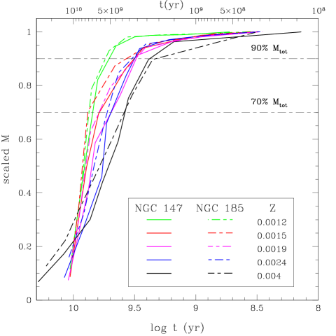
Figure 9: Cumulative SFH in the central $6\hbox to0.0pt{.\hss}^{\prime}5\times 6\hbox to0.0pt{.\hss}^{\prime}5$ regions of NGC = 147 and NGC 185.

In NGC 185, Martínez-Delgado & Aparicio (1998) determined a metallicity gradient within a $7\hbox to0.0pt{.\hss}^{\prime}2\times 7\hbox to0.0pt{.\hss}^{\prime}2$ region, on the basis of optical photometry. Additional photometry was used to derive the SFH (Martínez-Delgado, Aparicio & Gallart 1999). They found that the bulk of stellar mass was put in place early on, but star formation continued until at least $\sim 100$ Myr ago. They measured a mean SFR $\xi\approx 8.2\times 10^{-3}$ M_⊙ yr^-1 between 1–15 Gyr ago, and $\xi\approx 6.6\times 10^{-4}$ M_⊙ yr^-1 over the most recent Gyr. The most recent star formation is confined to the central $150\times 90$ pc². The results we obtained in an entirely different way are remarkably consistent with theirs; star formation sharply peaked $\sim 8$ Gyr ago, but star formation lasted until $\sim 200$ Myr ($\log t\approx 8.3$) $<170$ pc from the centre of NGC 185. The only discrepancy is that our SFRs are about twice their values. Like for NGC 147, Davidge (2005) used near-IR photometry of AGB stars; he found that in NGC 185 the most recent significant star formation occurred $\sim 1$ Gyr ago, i.e. much more recently than in NGC 147.

We derived total stellar masses of $M\approx 1.16\times 10^{8}$ M_⊙ for NGC 147 and $M\approx 2.42\times 10^{8}$ M_⊙ for NGC 185. The latter is in excellent agreement with the total stellar mass of $M\sim 2\times 10^{8}$ M_⊙ derived by Davidge (2005) for NGC 185 on the basis of near-IR photometry and assuming a mass-to-light ratio $M/L=1$; Geha et al. (2010) adopted somewhat larger $M/L$ values and hence obtained $M\sim 5.6\times 10^{8}$ M_⊙ for NGC 147 and $M\sim 7.2\times 10^{8}$ M_⊙ for NGC 185, i.e. 3–4 times higher than our estimates. Weisz et al. (2014a) obtained $M\sim 0.6\times 10^{8}$ M_⊙ for NGC 147 and $M\sim 0.7\times 10^{8}$ M_⊙ for NGC 185, but these estimates do not include all of the galaxy and are therefore lower limits. Their NGC 147 field was roughly centred and covered $\approx 0.23$ of the half-light area, so we may expect the corrected total mass estimate to be a few times higher, i.e. closer to $2\times 10^{8}$ M_⊙; their NGC 185 fields covered an area of similar size to the half-light area but off-centre by 200–800 pc, so the corrected total mass estimate would again be higher by a factor of a few, i.e. $\sim 2\times 10^{8}$ M_⊙. On balance, therefore, our estimates of the total stellar mass seem to agree with other, independent estimates, or perhaps be lower by a factor of a few at most. We may have missed some mass residing outside of the area covered by the monitoring data, or in the very oldest stars – which do not pulsate that strongly and which are therefore difficult to identify and account for – but not dramatically. Moreover, since the variable star survey is incomplete due to crowding in the central field of NGC 185, this may lead to star formation rates that are underestimated.

Figure 9 shows the cumulative SFH, i.e. the build-up of stellar mass over cosmological time. It is clear that the peak of star formation occurred earlier in NGC 185 than it did in NGC 147. It is also clear that the recent star formation in NGC 185 is insignificant in terms of stellar mass. Weisz et al. (2014b) argued that galaxies in which at least 70% of the stellar mass was in place by the time of cosmic reionization, could be considered ‘fossil’ galaxies. According to that definition, NGC 147 and NGC 185 are not fossil galaxies, but have been actively evolving since cosmic reionization. Weisz et al. (2014b) determined that 70% of the stellar mass was in place by $\log t=9.76$ for NGC 147 and by $\log t=9.92$ for NGC 185. We find very similar timings: $\log t=9.71$ for NGC 147 and $\log t=9.90$ for NGC 185. Weisz et al. (2015) then went on to quantify quenching of galaxy evolution, by the time by which 90% of the stellar mass is in place. According to this definition, the quenching of star formation occurred around $\log t=9.43$ in NGC 147 and $\log t=9.56$ in NGC 185; we find $\log t=9.55$ and $\log t=9.56$, respectively, i.e. sooner but similar in a relative sense. However, this neglects the recent star formation in NGC 185 as it accounts for $\ll 10$% of the stellar mass. By their definition, even the Milky Way would be close to being quenched now. What does it mean if star formation is quenched? What it does not mean, apparently, is that star formation is excluded from happening.

Martínez-Delgado et al. (1999) argued that the ISM in dEs could be replenished by mass loss from dying earlier generations of stars, and retained and fuel further star formation, possibly in an episodic fashion. This would explain the recent star formation and presence of ISM in NGC 185. The lack of ISM in NGC 147, which is consistent with the absence of stars younger than 300 Myr, could be due to external processes such as ram pressure due to the gaseous halo of M 31. Indeed, NGC 147 is tidally distorted and must therefore have spent some time recently in close proximity to M 31. Geha et al. (2015) suggest that the orbit of NGC 185 has a larger pericenter as compared to NGC 147, allowing it to preserve radial gradients and maintain a small central reservoir of recycled gas. They interpret the differences in early-SFH to imply an earlier infall time into the M 31 environment for NGC 185 as compared to NGC 147. Arias et al. (2016) determined the likely orbits of NGC 147 and NGC 185 and used them to perform $N$-body simulations to follow their morphological evolution. They reproduced the tidal features seen in NGC 147 (but not in NGC 185); their models suggest NGC 147 and NGC 185 (and the Cass II satellite) have been a bound group for at least a Gyr, and that their masses are $6.1\times 10^{8}$ M_⊙ for NGC 147 and $6.6\times 10^{8}$ M_⊙ for NGC 185, similar to the aforementioned values.

It may also be possible, however, that NGC 185 became more centrally concentrated early on, preventing the removal of the ISM from its centre, whereas a more diffuse NGC 147 would have been more susceptible to tidal and ram pressure stripping even if it were on a similar orbit.

6 Summary of conclusions

We have applied the novel method of Javadi et al. (2011) using long-period variable AGB stars to derive the SFH in the M 31 satellite dwarf elliptical galaxies NGC 147 and NGC 185. Our main findings are:

• Star formation started earlier in NGC 185 than in NGC 147, peaking around 8.3 Gyr ago in NGC 185 and 7 Gyr ago in NGC 147.

• Star formation continued in NGC 185 over the past 6 Gyr, albeit at a much lower rate, until as recent as 200 Myr ago in the centre, but it ceased much earlier in the outskirts; in NGC 147, on the other hand, while star formation was significant between 3–6 Gyr ago, no star formation is seen for the past 300 Myr, and stars of all ages are more uniformly distributed.

• The total stellar mass is $>2.42\times 10^{8}$ M_⊙ for NGC 185 and $>1.16\times 10^{8}$ M_⊙ for NGC 147; the true values are unlikely to be higher by more than a factor of a few.

• Of the total stellar mass, 70% (90%) was in place by $\log t=9.90$ (9.56) in NGC 185 and by $\log t=9.71$ (9.55) in NGC 147.

• Our conclusions were obtained completely independently, using different data and a different method, yet they are corroborated by previous work.

• We thus confirm the possibility of a scenario in which NGC 147 was accreted into the environs of M 31 later than NGC 185, but that its current orbit takes it closer to M 31 explaining its lack of ISM, lack of recent star formation, and its tidal distortions as opposed to the ISM and recent star formation in the centre of NGC 185. Alternatively, NGC 185 may have become more centrally concentrated early on, while NGC 147 has not.

Appendix A Supplementary material

Here we present plots and parameterizations of the mass–luminosity, mass–age and mass–pulsation duration relations derived from the theoretical models of Marigo et al. (2008) and used in our analysis of the star formation histories of NGC 147 and NGC 185. The methodology and the case of $Z=0.0019$ and $\mu=24.15$ mag are presented in the main body of the paper (section 3, figure 4 and tables 1–3).

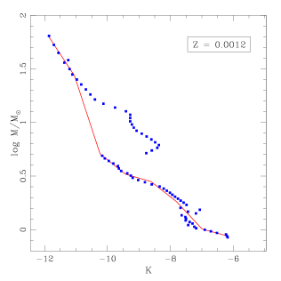
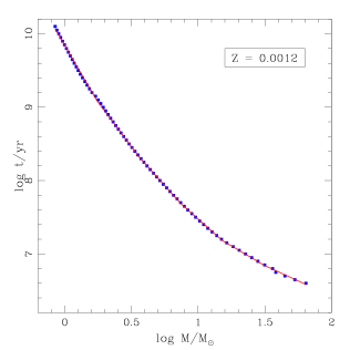
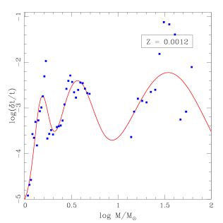
Figure 10: The dots refer to models from Marigo et al. (2008); (Left:) Mass–luminosity relation (in the $K$ band) for $Z=0.0012$ and a distance modulus of $\mu=0$ mag. The solid lines are linear spline fits, in which the function is interpolated over the super-AGB phase to massive red supergiants. (Middle:) Same, for the mass–age relation. (Right:) Same, for the mass–pulsation duration relation. The points show the ratio of pulsation duration to age, versus mass; the solid lines are multiple-Gaussian fits, interpolated over the super-AGB regime.

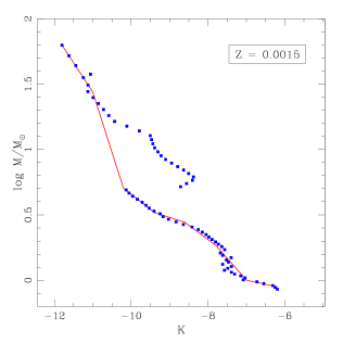
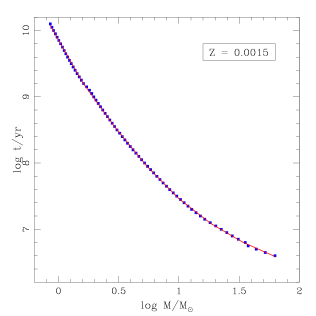
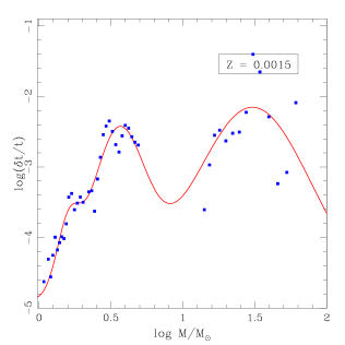
Figure 11: Same as Figure A1 for $Z=0.0015$.

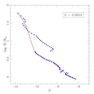
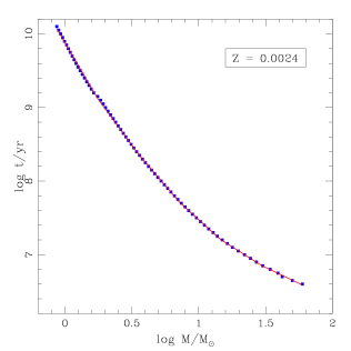
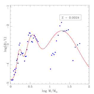
Figure 12: same as Figure A1 for $Z=0.0024$.

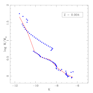
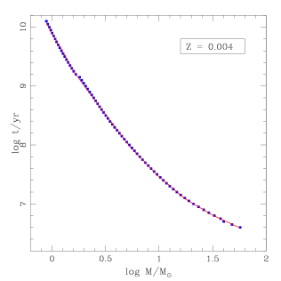
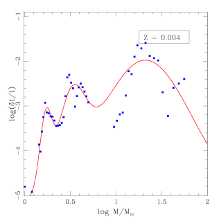
Figure 13: same as Figure A1 for $Z=0.004$.

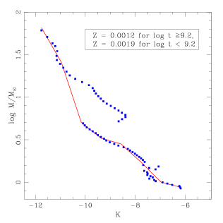
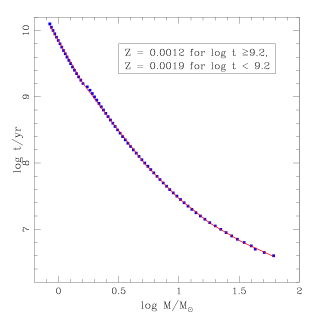
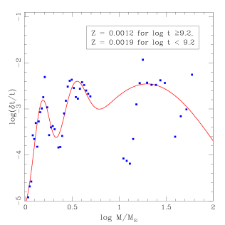
Figure 14: Same as Figure A1 with $Z=0.0012$ for $\log t\geq 9.2$ and $Z=0.0019$ for $\log t<9.2$.

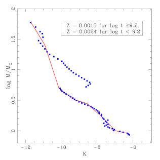
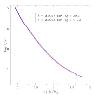
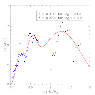
Figure 15: Same as Figure A1 with $Z=0.0015$ for $\log t\geq 9.2$ and $Z=0.0024$ for $\log t<9.2$.

Table 5: Relation between birth mass and $K$-band magnitude, $\log M=aK+b$, for a distance modulus of $\mu=0$ mag.

$a$	$b$	validity range
$Z=0.0012$
$-0.447\pm 0.086$	$-3.502\pm 0.985$	$K\leq-11.051$
$-0.897\pm 0.084$	$-8.476\pm 0.904$	$-11.051<K\leq-10.238$
$-0.233\pm 0.075$	$-1.683\pm 0.737$	$-10.238<K\leq-9.426$
$-0.085\pm 0.071$	$-0.286\pm 0.643$	$-9.426<K\leq-8.614$
$-0.231\pm 0.062$	$-1.542\pm 0.503$	$-8.614<K\leq-7.802$
$-0.315\pm 0.053$	$-2.198\pm 0.392$	$-7.802<K\leq-6.989$
$-0.080\pm 0.063$	$-0.553\pm 0.419$	$K>-6.989$
$Z=0.0015$
$-0.447\pm 0.071$	$-3.477\pm 0.808$	$K\leq-11.006$
$-0.918\pm 0.066$	$-8.667\pm 0.698$	$-11.006<K\leq-10.204$
$-0.232\pm 0.050$	$-1.663\pm 0.486$	$-10.204<K\leq-9.401$
$-0.094\pm 0.047$	$-0.362\pm 0.426$	$-9.401<K\leq-8.599$
$-0.219\pm 0.041$	$-1.436\pm 0.329$	$-8.599<K\leq-7.796$
$-0.333\pm 0.036$	$-2.330\pm 0.272$	$-7.796<K\leq-6.994$
$-0.062\pm 0.046$	$-0.432\pm 0.301$	$K>-6.994$
$Z=0.0024$
$-0.475\pm 0.070$	$-3.777\pm 0.787$	$K\leq-10.926$
$-0.911\pm 0.061$	$-8.538\pm 0.645$	$-10.926<K\leq-10.143$
$-0.225\pm 0.063$	$-1.585\pm 0.612$	$-10.143<K\leq-9.359$
$-0.098\pm 0.060$	$-0.393\pm 0.536$	$-9.359<K\leq-8.576$
$-0.253\pm 0.051$	$-1.722\pm 0.412$	$-8.576<K\leq-7.792$
$-0.256\pm 0.042$	$-1.743\pm 0.308$	$-7.792<K\leq-7.009$
$-0.147\pm 0.057$	$-0.985\pm 0.382$	$K>-7.009$
$Z=0.004$
$-0.544\pm 0.087$	$-4.621\pm 0.971$	$K\leq-10.819$
$-0.803\pm 0.074$	$-7.423\pm 0.771$	$-10.819<K\leq-10.083$
$-0.215\pm 0.073$	$-1.492\pm 0.707$	$-10.083<K\leq-9.347$
$-0.076\pm 0.070$	$-0.194\pm 0.634$	$-9.347<K\leq-8.610$
$-0.321\pm 0.061$	$-2.304\pm 0.501$	$-8.610<K\leq-7.874$
$-0.213\pm 0.052$	$-1.452\pm 0.396$	$-7.874<K\leq-7.138$
$-0.142\pm 0.071$	$-0.949\pm 0.489$	$K>-7.138$
$Z=0.0012$ for $\log t\geq 9.2$ and $Z=0.0019$ for $\log t<9.2$
$-0.510\pm 0.079$	$-4.176\pm 0.891$	$K\leq-10.962$
$-0.886\pm 0.071$	$-8.298\pm 0.756$	$-10.962<K\leq-10.165$
$-0.235\pm 0.071$	$-1.687\pm 0.686$	$-10.165<K\leq-9.367$
$-0.084\pm 0.066$	$-0.270\pm 0.599$	$-9.367<K\leq-8.568$
$-0.267\pm 0.058$	$-1.834\pm 0.467$	$-8.568<K\leq-7.772$
$-0.294\pm 0.052$	$-2.050\pm 0.385$	$-7.772<K\leq-6.975$
$-0.079\pm 0.063$	$-0.545\pm 0.416$	$K>-6.975$
$Z=0.0015$ for $\log t\geq 9.2$ and $Z=0.0024$ for $\log t<9.2$
$-0.478\pm 0.073$	$-3.810\pm 0.827$	$K\leq-10.922$
$-0.903\pm 0.063$	$-8.458\pm 0.669$	$-10.922<K\leq-10.133$
$-0.225\pm 0.065$	$-1.579\pm 0.633$	$-10.133<K\leq-9.345$
$-0.095\pm 0.062$	$-0.365\pm 0.556$	$-9.345<K\leq-8.556$
$-0.262\pm 0.053$	$-1.795\pm 0.429$	$-8.556<K\leq-7.768$
$-0.303\pm 0.051$	$-2.114\pm 0.381$	$-7.768<K\leq-6.979$
$-0.064\pm 0.064$	$-0.444\pm 0.425$	$K>-6.979$

Table 6: Relation between age and birth mass, $\log t=a\log M+b$.

$a$	$b$	validity range
$Z=0.0012$
$-3.109\pm 0.033$	$9.842\pm 0.003$	$\log{M}\leq 0.241$
$-2.433\pm 0.032$	$9.678\pm 0.013$	$0.241<\log{M}\leq 0.555$
$-2.043\pm 0.034$	$9.462\pm 0.024$	$0.555<\log{M}\leq 0.868$
$-1.618\pm 0.039$	$9.093\pm 0.040$	$0.868<\log{M}\leq 1.181$
$-1.074\pm 0.046$	$8.451\pm 0.061$	$1.181<\log{M}\leq 1.495$
$-0.833\pm 0.060$	$8.090\pm 0.097$	$\log{M}>1.495$
$Z=0.0015$
$-3.216\pm 0.030$	$9.860\pm 0.002$	$\log{M}\leq 0.198$
$-2.511\pm 0.028$	$9.720\pm 0.009$	$0.198<\log{M}\leq 0.465$
$-2.238\pm 0.030$	$9.593\pm 0.018$	$0.465<\log{M}\leq 0.732$
$-1.850\pm 0.033$	$9.310\pm 0.028$	$0.732<\log{M}\leq 0.998$
$-1.413\pm 0.038$	$8.873\pm 0.042$	$0.998<\log{M}\leq 1.265$
$-1.063\pm 0.043$	$8.430\pm 0.060$	$1.265<\log{M}\leq 1.531$
$-0.801\pm 0.054$	$8.030\pm 0.088$	$\log{M}>1.531$
$Z=0.0024$
$-3.100\pm 0.035$	$9.881\pm 0.004$	$\log{M}\leq 0.245$
$-2.479\pm 0.033$	$9.728\pm 0.013$	$0.245<\log{M}\leq 0.551$
$-2.128\pm 0.035$	$9.535\pm 0.025$	$0.551<\log{M}\leq 0.857$
$-1.649\pm 0.040$	$9.124\pm 0.040$	$0.857<\log{M}\leq 1.163$
$-1.156\pm 0.047$	$8.552\pm 0.061$	$1.163<\log{M}\leq 1.469$
$-0.862\pm 0.061$	$8.119\pm 0.097$	$\log{M}>1.469$
$Z=0.004$
$-3.207\pm 0.045$	$9.904\pm 0.004$	$\log{M}\leq 0.207$
$-2.470\pm 0.041$	$9.751\pm 0.014$	$0.207<\log{M}\leq 0.465$
$-2.398\pm 0.043$	$9.718\pm 0.025$	$0.465<\log{M}\leq 0.723$
$-1.901\pm 0.047$	$9.358\pm 0.040$	$0.723<\log{M}\leq 0.982$
$-1.559\pm 0.053$	$9.023\pm 0.059$	$0.982<\log{M}\leq 1.240$
$-1.083\pm 0.062$	$8.432\pm 0.084$	$1.240<\log{M}\leq 1.499$
$-0.846\pm 0.078$	$8.076\pm 0.126$	$\log{M}>1.499$
$Z=0.0012$ for $\log t\geq 9.2$ and $Z=0.0019$ for $\log t<9.2$
$-3.180\pm 0.041$	$9.845\pm 0.003$	$\log{M}\leq 0.193$
$-2.428\pm 0.038$	$9.699\pm 0.012$	$0.193<\log{M}\leq 0.459$
$-2.312\pm 0.039$	$9.646\pm 0.023$	$0.459<\log{M}\leq 0.724$
$-1.854\pm 0.044$	$9.314\pm 0.037$	$0.724<\log{M}\leq 0.990$
$-1.451\pm 0.050$	$8.915\pm 0.055$	$0.990<\log{M}\leq 1.255$
$-1.063\pm 0.057$	$8.429\pm 0.079$	$1.255<\log{M}\leq 1.521$
$-0.834\pm 0.072$	$8.080\pm 0.117$	$\log{M}>1.521$
$Z=0.0015$ for $\log t\geq 9.2$ and $Z=0.0024$ for $\log t<9.2$
$-3.183\pm 0.040$	$9.860\pm 0.003$	$\log{M}\leq 0.195$
$-2.437\pm 0.037$	$9.715\pm 0.012$	$0.195<\log{M}\leq 0.459$
$-2.345\pm 0.039$	$9.672\pm 0.022$	$0.459<\log{M}\leq 0.722$
$-1.868\pm 0.043$	$9.328\pm 0.036$	$0.722<\log{M}\leq 0.985$
$-1.478\pm 0.049$	$8.944\pm 0.054$	$0.985<\log{M}\leq 1.249$
$-1.082\pm 0.056$	$8.448\pm 0.077$	$1.249<\log{M}\leq 1.512$
$-0.842\pm 0.070$	$8.086\pm 0.114$	$\log{M}>1.512$

Table 7: Relation between the relative pulsation duration and birth mass, $\log(\delta t/t)=D+\Sigma_{i=1}^{3}a_{i}\exp\left[-(\log M[{\rm M}_{\odot}]-b_{i})^{2}/2c_{i}^{2}\right]$.

$D$	$i$	$a$	$b$	$c$
$Z=0.0012$
$-5.2$	1	1.955	0.173	0.074
	2	2.545	0.545	0.196
	3	2.936	1.539	0.429
$Z=0.0015$
$-4.9$	1	0.850	0.202	0.080
	2	2.265	0.547	0.188
	3	2.748	1.483	0.410
$Z=0.0024$
$-4.8$	1	1.267	0.222	0.064
	2	1.831	0.529	0.147
	3	2.567	1.302	0.427
$Z=0.004$
$-5.2$	1	1.510	0.229	0.065
	2	1.702	0.508	0.149
	3	3.258	1.320	0.519
$Z=0.0012$ for $\log t\geq 9.2$ and $Z=0.0019$ for $\log t<9.2$
$-6.5$	1	2.020	0.175	0.083
	2	1.455	0.519	0.126
	3	4.011	1.295	0.816
$Z=0.0015$ for $\log t\geq 9.2$ and $Z=0.0024$ for $\log t<9.2$
$-5.2$	1	1.240	0.213	0.086
	2	1.631	0.520	0.133
	3	2.944	1.265	0.522

References

- [Arias et al.(2016)] Arias V., et al., 2016, MNRAS, 456, 1654
- [Battinelli & Demers (2006)] Battinelli P., Demers S., 2006, A&A, 447, 473
- [Bertelli et al.(1994)] Bertelli G., Bressan A., Chiosi C., Fagotto F., Nasi E., 1994, A&AS, 106, 275
- [Crnojević et al.(2014)] Crnojević D., et al., 2014, MNRAS, 445, 3862
- [Davidge (1994)] Davidge T. J., 1994, AJ, 108, 2123
- [Davidge (2005)] Davidge T. J., 2005, AJ, 130, 2087
- [De Looze et al.(2016)] De Looze I., et al., 2016, MNRAS in press (arXiv:1604.06593)
- [Ferguson & Mackey (2016)] Ferguson A. M. N., Mackey A. D., 2016, in: “Tidal Streams in the Local Group and beyond”, Astrophysics and Space Science Library (Springer), Vol. 420, p.191
- [Geha et al.(2010)] Geha M. C., van der Marel R. P., Guhathakurta P., Gilbert K. M., Kalirai J., Kirby E. N., 2010, ApJ, 711, 361
- [Geha et al.(2015)] Geha M. C., Weisz D., Grocholski A., Dolphin A., van der Marel R. P., Guhathakurta P., 2015, ApJ, 811, 114
- [Girardi & Marigo (2007)] Girardi L., Marigo P., 2007, A&A, 462, 237
- [Girardi et al.(2010)] Girardi L., et al., 2010, ApJ, 724, 1030
- [Han et al.(1997)] Han M., et al., 1997, AJ, 113, 1001
- [Ho et al.(2015)] Ho N., Geha M., Tollerud E. J., Zinn R., Guhathakurta P., Vargas L. C., 2015, ApJ, 798, 77
- [Iben & Renzini (1983)] Iben I. Jr., Renzini A., 1983, ARA&A, 21, 271
- [Javadi, van Loon & Mirtorabi (2011)] Javadi A., van Loon J. Th., Mirtorabi M. T., 2011, MNRAS, 414, 3394
- [Javadi et al.(2016)] Javadi A., van Loon J. Th., Khosroshahi H. G., Tabatabaei F., Golshan R. H., Rashidi M., 2016, MNRAS, submitted
- [Kang et al.(2005)] Kang A., Sohn Y.-J., Rhee J., Shin M., Chun M.-S., Kim H.-I., 2005, A&A, 437, 61
- [Lorenz et al.(2011)] Lorenz D., Lebzelter T., Nowotny W., Telting J., Kerschbaum F., Olofsson H., Schwarz H.E., 2011, A&A, 532, 78
- [Marigo et al.(2008)] Marigo P., Girardi L., Bressan A., Groenewegen M.A.T., Silva L., Granato G. L., 2008, A&A, 482, 883
- [Marleau, Noriega-Crespo & Misselt (2010)] Marleau F. R., Noriega-Crespo A., Misselt K.A., 2010, ApJ, 713, 992
- [Martínez-Delgado & Aparicio (1998)] Martínez-Delgado D., Aparicio A., 1998, AJ, 115, 1462
- [Martínez-Delgado, Aparicio & Gallart (1999)] Martínez-Delgado D., Aparicio A., Gallart C., 1999, AJ, 118, 2229
- [McConnachie et al.(2005)] McConnachie A. W., Irwin M. J., Ferguson A. M. N., Ibata R. A., Lewis G. F., Tanvir N., 2005, MNRAS, 356, 979
- [Nowotny et al.(2003)] Nowotny W., Kerschbaum F., Olofsson H., Schwarz H. E., 2003, A&A, 403, 93
- [Sohn et al.(2006)] Sohn Y.-J., Kang A., Rhee J., Shin M., Chun M.-S., Kim H.-I., 2006, A&A, 445, 69
- [Rezaeikh et al.(2014)] Rezaeikh S., Javadi A., Khosroshahi H., van Loon, J. Th., 2014, MNRAS, 445, 2214
- [van den Bergh (1998)] van den Bergh S., 1998, AJ, 116, 1688
- [Vargas, Geha & Tollerud (2014)] Vargas L. C., Geha M. C., Tollerud E. J., 2014, ApJ, 790, 73
- [Watkins, Evans & van de Ven (2013)] Watkins L. L., Evans N. W., van de Ven G., 2013, MNRAS, 430, 971
- [Weisz et al.(2014a)] Weisz D. R., Dolphin A. E., Skillman E. D., Holtzman J., Gilbert K. M., Dalcanton J. J., Williams B. F., 2014a, ApJ, 789, 147
- [Weisz et al.(2014b)] Weisz D. R., Dolphin A. E., Skillman E. D., Holtzman J., Gilbert K. M., Dalcanton J. J., Williams B. F., 2014b, ApJ, 789, 148
- [Weisz et al.(2015)] Weisz D. R., Dolphin A. E., Skillman E. D., Holtzman J., Gilbert K. M., Dalcanton J. J., Williams B. F., 2015, ApJ, 804, 136
- [Welch, Sage & Mitchell (1998)] Welch G. A., Sage L. J., Mitchell G. F., 1998, ApJ, 499, 209
- [Young & Lo 1997] Young L. M., Lo K. Y., 1997, ApJ, 476, 127