Turbulent diffusion of chemically reacting flows: theory and numerical simulations

Abstract

The theory of turbulent diffusion of chemically reacting gaseous admixtures developed previously (Phys. Rev. E 90, 053001, 2014) is generalized for large yet finite Reynolds numbers, and the dependence of turbulent diffusion coefficient versus two parameters, the Reynolds number and Damköhler number (which characterizes a ratio of turbulent and reaction time scales) is obtained. Three-dimensional direct numerical simulations (DNS) of a finite thickness reaction wave for the first-order chemical reactions propagating in forced, homogeneous, isotropic, and incompressible turbulence are performed to validate the theoretically predicted effect of chemical reactions on turbulent diffusion. It is shown that the obtained DNS results are in a good agreement with the developed theory.

I Introduction

Effect of chemical reactions on turbulent transport is of great importance in many applications ranging from atmospheric turbulence and transport of pollutants to combustion processes (see, e.g., CSA80 ; BLA97 ; F03 ; P04 ; SP06 ; ZA08 ; ML08 ; CRC ). For instance, significant influence of combustion on turbulent transport is well known CRC ; L85 ; Br95 ; PECS10 ; SB11 ; AR17 to cause the so-called counter-gradient scalar transport, i.e. a flux of products from unburnt to burnt regions of a premixed flame. In its turn, the counter-gradient transport can substantially reduce the flame speed SL13 ; SL14 ; SL15 and, therefore, is of great importance for calculations of burning rate and plays a key role in the premixed turbulent combustion.

It is worth remembering, however, that the counter-gradient transport appears to be an indirect manifestation of the influence of chemical reactions on turbulent fluxes, as this manifestation is controlled by density variations due to heat release in combustion reactions, rather than by the reactions themselves. As far as the straightforward influence of reactions on turbulent transport Corr is concerned, such effects have yet been addressed in a few studies CRC ; BD17 ; L33 of premixed flames. Because the easiest way to studying such a straightforward influence consists in investigating a constant-density reacting flow, the density is considered to be constant in the present paper.

The effect of chemical reactions on turbulent diffusion of chemically reacting gaseous admixtures in a developed turbulence has been studied analytically using a path-integral approach for a delta-correlated in time random velocity field EKR98 . This phenomenon also has been recently investigated applying the spectral-tau approach that is valid for large Reynolds and Peclet numbers EKLR14 . These studies have demonstrated that turbulent diffusion of the reacting species can be strongly suppressed with increasing Damköhler number, ${\rm Da}=\tau_{0}/\tau_{c}$, that is a ratio of turbulent, $\tau_{0}$, and chemical, $\tau_{c}$, time scales.

The dependence of turbulent diffusion coefficient, $D_{T}$, versus the turbulent Damköhler number obtained theoretically in EKLR14 , was validated using results of mean-field simulations (MFS) of a reactive front propagating in a turbulent flow BH11 . In these simulations, the mean speed, $s_{{}_{T}}$, of the planar one-dimensional reactive front was determined using numerical solution of the Kolmogorov-Petrovskii-Piskunov (KPP) equation KPP37 or the Fisher equation F37 . This mean-field equation was extended in BH11 to take into account memory effects of turbulent diffusion when the turbulent time was much larger than the characteristic chemical time. Turbulent diffusion coefficients as a function of ${\rm Da}$ were determined numerically in BH11 using the obtained function $s_{{}_{T}}({\rm Da})$ and invoking the well-known expression, $s_{{}_{T}}=2(D_{T}/\tau_{c})^{1/2}$. The theoretical dependence $D_{T}({\rm Da})$ derived in EKLR14 was in a good agreement with the numerical results of MFS BH11 .

In the present study we have generalized the theory EKLR14 of turbulent diffusion in reacting flows for finite Reynolds numbers and have obtained the dependence of turbulent diffusion coefficient versus two parameters, the Reynolds number and Damköhler number. The generalized theory has been validated by comparing its predictions with the three-dimensional direct numerical simulations (DNS) of the reaction wave propagating in a homogeneous isotropic and incompressible turbulence for a wide range of ratios of the wave speed to the r.m.s. turbulent velocity and different Reynolds numbers.

It is worth stressing that the previous validation of the original theory by MFS EKLR14 and present validation of the generalized theory by DNS complement each other, because they were performed using different methods. Indeed, the previous validation EKLR14 was performed by evaluating $D_{T}$ using numerical data BH11 on the mean reaction front speed obtained by solving a statistically planar one-dimensional mean KPP equation, with such a MFS method implying spatial uniformity of the turbulent diffusion coefficient. On the contrary, in the present work, $D_{T}$ is straightforwardly extracted from DNS data obtained by numerically integrating unsteady three-dimensional Navier-Stokes and reaction-diffusion equations, with eventual spatial variations in the turbulent diffusion coefficient being addressed.

This paper is organised as follows. The generalized theory is described in Section II. DNS performed to validate the theory are described in Section III. Subsequently, validation results are discussed in Section IV, and concluding remarks are given in Section V.

II Effect of chemistry on turbulent diffusion

The goal of this section is to generalize the theory EKLR14 by considering turbulent flows characterized by large, but finite Reynolds numbers. It is worth stressing that neither the original theory EKLR14 nor its generalization have specially been developed to study combustion. On the contrary, while the theory addresses a wide class of turbulent reacting flows, certain assumptions of the theory do not hold in premixed flames. Nevertheless, as will be shown in subsequent sections, the theoretical predictions are valid under a wider range of conditions than originally assumed and, in particular, under conditions associated with the straightforward influence of chemical reactions on turbulence in flames.

II.1 Governing equations

Equation for the scalar field in the incompressible chemically reacting turbulent flow reads:

$$\frac{\partial c}{\partial t}+({\bm{v}}\cdot{\bm{\nabla}})c=W(c)+D\Delta c,$$ (1)

where $c(t,{\bm{x}})$ is a scalar field, ${\bm{v}}(t,{\bm{x}})$ is the instantaneous fluid velocity field, $D$ is a constant diffusion coefficient based on molecular Fick’s law, $W(c)$ is the source (or sink) term. The function $W(c)$ is usually chosen according to the Arrhenius law (to be given in the next section). We consider a simplified model of a single-step reaction typically used in numerical simulations of turbulent combustion.

The velocity ${\bm{v}}$ of the fluid is determined by the Navier-Stokes equation:

$${\partial{\bm{v}}\over\partial t} + ({\bm{v}}\cdot{\bm{\nabla}}){\bm{v}}=-{1\over\rho}{\bm{\nabla}}p+\nu\Delta{\bm{v}}+{\bm{f}},$$ (2)

where ${\bm{f}}$ is the external force to support turbulence, $\nu$ is the kinematic viscosity, $p$ and $\rho$ are the fluid pressure and density, respectively. For an incompressible flow the fluid density is constant.

II.2 Procedure of derivations of turbulent flux

To determine turbulent transport coefficients, Eq. (1) is averaged over an ensemble of turbulent velocity fields. In the framework of a mean-field approach, the scalar field $c$ is decomposed into the mean field, $\langle c\rangle$, and fluctuations, $c^{\prime}$, where $\langle c^{\prime}\rangle=0$, and angular brackets imply the averaging over the statistics of turbulent velocity field. The velocity field is decomposed in a similar fashion, ${\bm{v}}=\langle{\bm{U}}\rangle+{\bm{u}}$, assuming for simplicity vanishing mean fluid velocity, $\langle{\bm{U}}\rangle=0$, where ${\bm{u}}$ are the fluid velocity fluctuations.

Using the equation for fluctuations $c^{\prime}=c-\langle c\rangle$ of the scalar field and the Navier-Stokes equation for fluctuations ${\bm{u}}$ of the velocity field written in ${\bm{k}}$ space we derive equation for the second-order moment $\langle c^{\prime}\,{\bm{u}}\rangle_{\bm{k}}\equiv\langle c^{\prime}({\bm{k}})\,u_{i}(-{\bm{k}})\rangle$:

$$\frac{\partial\langle c^{\prime}\,u_{i}\rangle_{\bm{k}}}{\partial t}=-\left[\tau_{c}^{-1}+(\nu+D)k^{2}\right]\langle c^{\prime}\,u_{i}\rangle_{\bm{k}}+\hat{\cal N}\langle c^{\prime}\,u_{i}\rangle$$

$$\quad-\langle u_{i}\,u_{j}\rangle_{\bm{k}}\,\nabla_{j}\langle c\rangle,$$ (3)

where $\langle u_{i}\,u_{j}\rangle_{\bm{k}}\equiv\langle u_{i}({\bm{k}})\,u_{j}(-{\bm{k}})\rangle$, $\tau_{c}=\langle c\rangle/\langle W\rangle$ is the chemical time, $\langle W\rangle$ is the mean source function and $\hat{\cal N}\langle c^{\prime}\,u_{i}\rangle$ includes the third-order moments caused by the nonlinear terms:

$$\hat{\cal N}\langle c^{\prime}\,u_{i}\rangle=-\langle[{\bm{\nabla}\cdot}(c^{\prime}\,{\bm{u}})]\,u_{i}\rangle_{\bm{k}}-\langle c^{\prime}\,[({\bm{u}}\cdot{\bm{\nabla}})u_{i}]\rangle_{\bm{k}}$$

$$\quad-\langle c^{\prime}\,[\rho^{-1}\nabla_{i}p^{\prime}]\rangle_{\bm{k}}.$$ (4)

Here we follow the procedure of the derivation of the turbulent fluxes that is described in detail in EKLR14 , taking into account large yet finite Reynolds number. In particular, we use multi-scales approach (i.e., we separated fast and slow variables, where fast small-scale variables correspond to fluctuations and slow large-scale variables correspond to mean fields). Since the ratio of spatial density of species is assumed to be much smaller than the density of the surrounding fluid (i.e., small mass-loading parameter), there is only one-way coupling, i.e., no effect of species on the fluid flow. Due to the same reason the energy release (or absorbtion of energy) caused by chemical reactions is much smaller than the internal energy of the surrounding fluid. This implies that even small chemical time does not affect the fluid characteristics. Finally, we also assume that the deviations of the source term $W$ from its mean value $\langle W\rangle$ is not large. While such an assumption does not hold in a typical premixed turbulent flame CRC , we will see later that the theory well predicts the effect of the chemical reaction on turbulent transport even if difference in $W(c)$ and $\langle W\rangle(\langle c\rangle)$ is significant, as commonly occurs in the case of premixed combustion.

The equation for the second-order moment (3) includes the first-order spatial differential operators applied to the third-order moments $\hat{\cal N}\langle c^{\prime}\,u_{i}\rangle$. To close the system of equations it is necessary to express the third-order terms $\hat{\cal N}\langle c^{\prime}\,u_{i}\rangle$ through the lower-order moments $\langle c^{\prime}\,u_{i}\rangle_{\bm{k}}$ (see, e.g., O70 ; MY75 ; Mc90 ). We use the spectral $\tau$ approximation that postulates that the deviations of the third-order moments, $\hat{\cal N}\langle c^{\prime}\,u_{i}\rangle$, from the contributions to these terms afforded by the background turbulence, $\hat{\cal N}\langle c^{\prime}\,u_{i}\rangle^{(0)}$, can be expressed through the similar deviations of the second-order moments, $\langle c^{\prime}\,u_{i}\rangle_{\bm{k}}-\langle c^{\prime}\,u_{i}\rangle_{\bm{k}}^{(0)}$:

$$\hat{\cal N}\langle c^{\prime}\,u_{i}\rangle-\hat{\cal N}\langle c^{\prime}\,u_{i}\rangle^{(0)}=-{1\over\tau_{r}(k)}\,\Big{[}\langle c^{\prime}\,u_{i}\rangle_{\bm{k}}-\langle c^{\prime}\,u_{i}\rangle_{\bm{k}}^{(0)}\Big{]},$$

(5)

(see, e.g., O70 ; MY75 ; PFL76 ), where $\tau_{r}(k)$ is the scale-dependent relaxation time, which can be identified with the correlation time $\tau(k)$ of the turbulent velocity field for large Reynolds and Peclet numbers. The functions with the superscript $(0)$ correspond to the background turbulence with zero gradients of the mean scalar field. Validation of the $\tau$ approximation for different situations has been performed in various numerical simulations and analytical studies (see, e.g., BS05 ; RK07 ; RKKB11 ). When the gradients of the mean scalar field are zero, the turbulent flux vanishes, and the contributions of the corresponding fluctuations [the terms with the superscript (0)], vanish as well. Consequently, Eq. (5) reduces to $\hat{\cal N}\langle c^{\prime}\,u_{i}\rangle_{\bm{k}}=-\langle c^{\prime}({\bm{k}})\,u_{i}(-{\bm{k}})\rangle/\tau(k)$.

We also assume that the characteristic times of variation of the second-order moments are substantially larger than the correlation time $\tau(k)$ for all turbulence scales. This allows us to consider the steady-state solution of Eq. (3), that yields the following expression for the turbulent flux $\langle c^{\prime}\,u_{i}\rangle_{\bm{k}}=\langle c^{\prime}({\bm{k}})\,u_{i}(-{\bm{k}})\rangle$ in ${\bm{k}}$ space:

$$\langle c^{\prime}\,u_{i}\rangle_{\bm{k}}=-\tau_{\rm eff}(k)\,\langle u_{i}\,u_{j}\rangle_{\bm{k}}^{(0)}\,\nabla_{j}\langle c\rangle,$$ (6)

where $\tau_{\rm eff}(k)=\left[\tau_{c}^{-1}+(\nu+D)k^{2}+\tau^{-1}(k)\right]^{-1}$ is the effective time.

We consider isotropic and homogeneous background turbulence, $\langle u_{i}\,u_{j}\rangle_{\bm{k}}^{(0)}\equiv\langle u_{i}({\bm{k}})\,u_{j}(-{\bm{k}})\rangle$ (see, e.g., B53 ):

$$\langle u_{i}({\bm{k}})\,u_{j}(-{\bm{k}})\rangle={u_{0}^{2}\,E_{T}(k)\over 8\pi k^{2}}\Big{[}\delta_{ij}-{k_{i}\,k_{j}\over k^{2}}\Big{]},$$ (7)

where

$$E_{T}(k)={2\over 3k_{0}}\left(1-{\rm Re}^{-1/2}\right)^{-1}\left({k\over k_{0}}\right)^{-5/3},$$ (8)

is the energy spectrum function for $k_{0}\leq k\leq k_{0}{\rm Re}^{3/4}$, $\tau(k)=2\,\tau_{0}\,(k/k_{0})^{-2/3}$ is the turbulent correlation time, $k_{0}=\ell_{0}^{-1}$, and ${\rm Re}=\ell_{0}u_{0}/\nu\gg 1$ is the Reynolds number, $u_{0}$ is the characteristic turbulent velocity in the integral scale, $\ell_{0}$, of turbulence. For comparison of the theory with DNS we do not neglect the small ${\rm Re}^{-1/2}$ term in Eq. (8).

II.3 Turbulent flux

After integration in ${\bm{k}}$ space we obtain the expression for the turbulent flux, $\langle c^{\prime}\,{\bm{u}}\rangle$:

$$\langle c^{\prime}\,{\bm{u}}\rangle=\int\langle c^{\prime}\,u_{i}\rangle_{\bm{k}}\,d{\bm{k}}=-D_{T}\,{\bm{\nabla}}\langle c\rangle,$$ (9)

where the coefficient of turbulent diffusion $D_{T}$ of the scalar field is

$$D_{T}={D^{T}_{0}\over{\rm Da}}\,\left[1-{\Phi({\rm Da},{\rm Re},{\rm Pr})\over 1-{\rm Re}^{-1/2}}\right],$$ (10)

$D^{T}_{0}=\tau_{0}u_{0}^{2}/3$ is the characteristic value of the turbulent diffusion coefficient without chemical reactions, $\tau_{0}=\ell_{0}/u_{0}$ is the characteristic turbulent time, the function $\Phi({\rm Da},{\rm Re},{\rm Pr})$ is

$$\Phi({\rm Da},{\rm Re},{\rm Pr})=\int_{{\rm Re}^{-1/2}}^{1}\,{X^{2}+a({\rm Re},{\rm Pr})\over 2{\rm Da}X^{3}+X^{2}+a}\,dX,$$ (11)

the parameter $a({\rm Re},{\rm Pr})=2\left(1+{\rm Pr}^{-1}\right)/{\rm Re}$, and ${\rm Pr}=\nu/D$ is the Prandtl number.

Evaluating approximately the integral in Eq. (11) by expanding the expression in the integral over small parameter $a({\rm Re},{\rm Pr})$ for large yet finite Reynolds numbers, we obtain the following dependence of turbulent diffusion coefficient versus Damköhler and Reynolds numbers:

$$D_{T} = {D^{T}_{0}\over{\rm Da}}\,\left[1-{1\over 2{\rm Da}\left[1-{\rm Re}^{-1/2}\right]}\,\ln{1+2{\rm Da}\over 1+2{\rm Da}\,{\rm Re}^{-1/2}}\right]$$ (12)

$$-2D^{T}_{0}\,\left(1+{\rm Pr}^{-1}\right)\,{\ln{\rm Re}\over{\rm Re}}.$$

In the limit of extremely large Reynolds numbers, we recover the result for the function $D_{T}({\rm Da})$ obtained in EKLR14 :

$$D_{T} = {D^{T}_{0}\over{\rm Da}}\,\left[1-{\ln(1+2{\rm Da})\over 2{\rm Da}}\right].$$

It follows from Eq. (12) that for small Damköhler numbers, ${\rm Da}\ll 1$, the function $D_{T}({\rm Da})$ is given by:

$$D_{T} = D^{T}_{0}\,\biggl{[}1-{4{\rm Da}\over 3}-2D^{T}_{0}\,\left(1+{\rm Pr}^{-1}\right)\,{\ln{\rm Re}\over{\rm Re}}$$ (14)

$$+{\rm Re}^{-1/2}\biggr{]},$$

while for large Damköhler numbers, $1\ll{\rm Da}\ll{\rm Re}^{1/2}$, it is

$$D_{T}={D^{T}_{0}\over{\rm Da}}\,\left[1-{\ln 2{\rm Da}\over 2{\rm Da}}-2\,\left(1+{\rm Pr}^{-1}\right)\,{{\rm Da}\,\ln{\rm Re}\over{\rm Re}}\right],$$

(15)

and for very large Damköhler numbers, $1\ll{\rm Re}^{1/2}\ll{\rm Da}$, it is

$$D_{T}={D^{T}_{0}\over{\rm Da}}\,\left[1-2\,\left(1+{\rm Pr}^{-1}\right)\,{{\rm Da}\,\ln{\rm Re}\over{\rm Re}}\right].$$ (16)

Equations (15) and (16) show that turbulent diffusion of particles or gaseous admixtures for a large Damköhler number, ${\rm Da}\gg 1$ is strongly reduced, i.e., $D_{T}=D_{0}^{T}/{\rm Da}=\tau_{c}u_{0}^{2}/3$. This implies that the turbulent diffusion for a large turbulent Damköhler number is determined by the chemical time. The underlying physics of the strong reduction of turbulent diffusion is quite transparent. For a simple first-order chemical reaction $A\to B$ the species $A$ of the reactive admixture are consumed and their concentration decreases much faster during the chemical reaction, so that the usual turbulent diffusion based on the turbulent time $\tau_{0}\gg\tau_{c}$, does not contribute to the mass flux of a reagent $A$.

III DNS model

Direct numerical simulations of a finite thickness reaction wave propagation in forced, homogeneous, isotropic, and incompressible turbulence for the first-order chemical reactions, were performed in a fully periodic rectangular box of size of $L_{x}\times L_{y}\times L_{z}$ using a uniform rectangular mesh of $N_{x}\times N_{y}\times N_{z}$ points and a simplified in-house solver YYB12 developed for low-Mach-number reacting flows. Contrary to recent DNS studies by two of the present authors YLB14 ; YBL15 that addressed self-propagation of an infinitely thin interface by solving a level set equation, the present simulations deal with a wave of a finite thickness, modelled with Eq. (1) for a single progress variable $c$ ($c=0$ and 1 in reactants and products, respectively), while the Navier-Stokes equation (2) was numerically integrated in both cases.

To mimic a highly non-linear dependence of the reaction rate $W$ on the scalar field $c$ in a typical premixed flame characterized by significant variations in the density $\rho$ and temperature $T$, the following expression,

$$W={1-c\over\tau_{{}_{R}}\,(1+\tau)}\exp\left[-{{\rm Ze}\,(1+\tau)^{2}\over\tau\,(1+c\,\tau)}\right],$$ (17)

was invoked in the present constant-density simulations. Here, $\tau_{{}_{R}}$ is a reaction time scale, while parameters $Ze=6.0$ and $\tau=6.0$ are counterparts of the Zeldovich number ${\rm Ze}=E_{a}(T_{b}-T_{u})/RT_{b}^{2}$ and heat-release factor $(\rho_{u}-\rho_{b})/\rho_{b}$, respectively, which are widely used in the combustion theory CRC ; L85 ; Br95 , with subscripts $u$ and $b$ designating unburned and burned mixtures, respectively. Indeed, substitution of $c=(T-T_{u})/(T_{b}-T_{u})$ into exponent in Eq. (17) results in the classical Arrhenius law

$$W={1-c\over\tau_{{}_{R}}\,(1+\tau)}\exp\left(-\frac{E_{a}}{RT}\right),$$ (18)

i.e. Eq. (17) does allow us to mimic behavior of reaction rate in a flame by considering constant-density reacting flows. It is worth remembering that a simplification of a constant density is helpful for studying the straightforward influence of chemical reactions on turbulent transport, as already pointed out in Sect. I.

The speed $S_{{}_{L}}$ of the propagation of the reaction wave in the laminar flow, the wave thickness $\delta_{{}_{F}}=D/S_{{}_{L}}$, the wave time scale $\tau_{{}_{F}}=\delta_{{}_{F}}/S_{{}_{L}}$ were varied by changing the diffusion coefficient $D$ and the reaction time scale $\tau_{{}_{R}}$, which were constant input parameters for each DNS run. The speed $S_{{}_{L}}$ was determined by numerically solving one-dimentional Eq. (1) with ${\bm{v}}=0$.

The present DNS are similar to DNS discussed in detail in YLB14 ; YBL15 , except for substitution of a level set equations used in YLB14 ; YBL15 by Eqs. (1) and (17). Therefore, we will restrict ourselves to a very brief summary of the simulations. A more detailed discussion of the simulations can be found in recent papers PRE17RA ; PoF17RA .

The boundary conditions were periodic not only in transverse directions $y$ and $z$, but also in direction $x$ normal to the mean wave surface. In other words, when the reaction wave reached the left boundary ($x=0$) of the computational domain, the identical reaction wave entered the domain through its right boundary ($x=L_{x}$).

The initial turbulence field was generated by synthesizing prescribed Fourier waves (YB14, ) with an initial rms velocity $u_{0}$ and the forcing scale $\ell_{\rm f}=L/4$, where $L=L_{y}=L_{z}=L_{x}/4$ is the width of the computational domain. Subsequently, a forcing function ${\bm{f}}$, see Eq. (2), was invoked to maintain statically stationary turbulence following the method described in Ref. GLMA95 . As shown earlier YLB14 ; YBL15 , (i) the rms velocity $u_{0}$ was maintained as the initial value, (ii) the normalized dissipation rate $\langle\varepsilon\rangle\ell_{\rm f}/u_{0}^{3}$ averaged over the computational domain fluctuated slightly above 3/2 after a short period ($t<\tau_{\rm f}=\ell_{\rm f}/u_{0}$) of rapid transition from the initial artificially synthesized flow to the fully developed turbulence, (iii) the forced turbulence achieved good statistical homogeneity and isotropy over the entire domain, and (iv) the energy spectrum showed a sufficiently wide range of the Kolmogorov scaling ($-5/3$) at the Reynolds number, ${\rm Re}\equiv u_{0}\ell_{\rm f}/\nu=200$, based on the scale $\ell_{\rm f}$ (see Fig. 1).

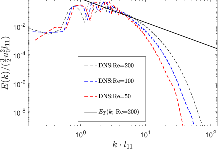
Figure 1: Spectrum of turbulent kinetic energy

Table 1: DNS cases.

Case	${\rm Re}$	${\rm Re}_{\lambda}$	$\eta/\Delta x$	$S_{{}_{L}}/u_{0}$	$\ell_{11}/\delta_{{}_{F}}$	${\rm Da}_{{}_{\rm DNS}}$
1	50	18	0.68	0.1	2.1	0.2
2	50	18	0.68	0.2	2.1	0.4
3	50	18	0.68	0.5	2.1	1.0
4	50	18	0.68	1.0	2.1	2.1
5	50	18	0.68	2.0	2.1	4.1
6	100	30	0.86	0.1	3.7	0.4
7	100	30	0.86	0.2	3.7	0.7
8	100	30	0.86	0.5	3.7	1.9
9	100	30	0.86	1.0	3.7	3.7
10	100	30	0.86	2.0	3.7	7.5
11	200	45	1.06	0.1	6.7	0.7
12	200	45	1.06	0.2	6.7	1.3
13	200	45	1.06	0.5	6.7	3.4
14	200	45	1.06	1.0	6.7	6.7
15	200	45	1.06	2.0	6.7	13.5

In order to study a fully-developed reaction wave, a planar wave $c(\bm{x},t=0)=c_{L}(\xi)$ was initially ($t=0$) released at $x^{0}=L_{x}/2$ such that $\int_{-\infty}^{0}c_{L}(\xi)\mathrm{d}\xi=\int_{0}^{\infty}[1-c_{L}(\xi)]\mathrm{d}\xi$ and $\xi=x-x^{0}$, where, $c_{L}(\xi)$ is the pre-computed laminar-wave profile. Subsequently, evolution of this field $c(\bm{x},t)$ was simulated by solving Eq. (1). To enable periodic propagation of $c$ field along $x$-direction, the field is extrapolated outside the axial boundaries of the computational domain at each time step $t^{n}$ as follows; $c(x^{\prime},y,z,t^{n})=c(x,z,t^{n})$, where $x^{\prime}=x+I\textrm{L}_{x}$ and $I$ is an arbitrary (positive or negative) integer number. Consequently, Eq. (1) is solved in the interval $x^{\prime}\in[\zeta(t^{n})-\Delta,\zeta(t^{n})+\Delta]$, where $\zeta(t^{n})$ is the mean coordinate of a reaction wave on the $x^{\prime}$-axis and $\Delta=0.45\textrm{L}_{x}$ in order to avoid numerical artifacts in the vicinity of $x^{\prime}=\zeta(t^{n})\pm 0.5\textrm{L}_{x}$. In two remaining regions, i.e. $x^{\prime}\in[\zeta(t^{n})-0.5\textrm{L}_{x},\zeta(t^{n})-\Delta]$ and $x^{\prime}\in[\zeta(t^{n})+\Delta,\zeta(t^{n})+0.5\textrm{L}_{x}]$, the scalar $c(t^{n})$ is set equal to zero (fresh reactants) and unity (products), respectively, because the entire flame brush is always kept within the interval of $x^{\prime}\in[\zeta(t^{n})-\Delta,\zeta(t^{n})+\Delta]$ in the present simulations. Finally, the obtained solution $c(x^{\prime},y,z,t^{n})$ is translated back to the $x$-coordinate (see for details, PRE17RA ; PoF17RA ).

Three turbulent fields were generated by specifying three different initial turbulent Reynolds numbers ${\rm Re}=50$, 100, and 200, which were increased by increasing the domain size $L$. The increase in $L$ resulted in increasing the longitudinal integral length scale $\ell_{11}$, the Taylor length scale $\lambda=\sqrt{15\nu u_{0}^{2}/\overline{\langle\varepsilon\rangle}}$, the Taylor scale Reynolds number ${\rm Re}_{\lambda}=u_{0}\lambda/\nu$, the turbulent time scale $\tau_{11}=\ell_{11}/u_{0}$, and, hence, the Damköhler number ${\rm Da_{{}_{\rm DNS}}}=\tau_{11}/\tau_{{}_{F}}$. Here, $\overline{\langle\varepsilon\rangle}$ is the dissipation rate averaged over volume (angle brackets) and time at $t>5\tau_{\rm f}$ (overbars). The simulation parameters are shown in Table I. Because a reaction wave does not affect turbulence in the case of constant density $\rho$ and viscosity $\nu$, the flow statistics were the same in all cases that had different $S_{{}_{L}}$, but the same ${\rm Re}$. It is worth noting that the longitudinal integral length scale $\ell_{11}$ reported in Table I and used to evaluate ${\rm Da_{{}_{\rm DNS}}}$ was averaged over the computational domain and time at $t>5\tau_{\rm f}$ and was lower than its initial value $\ell_{\rm f}=L/4$.

When the width $L$ was increased by a factor of two, the numbers $N_{x}$, $N_{y}=N_{x}/4$, and $N_{z}=N_{x}/4$ were also increased by a factor of two, i.e. $N_{x}=256$, 512, or 1024 at ${\rm Re}=50$, 100, or 200, respectively. Accordingly, in all cases, the Kolmogorov length scale $\eta=(\nu^{3}/\overline{\langle\varepsilon\rangle})^{1/4}$ was of the order of the grid cell size $\Delta x$, see Table I, thus, indicating sufficient grid resolution. Capability of the used grids for well resolving not only the Kolmogorov eddies, but also the reaction wave was confirmed in separate (i) 1D simulations of planar laminar reaction waves and (ii) 2D simulations YBB15 of laminar flames subject to hydrodynamic instability LL . Moreover, the resolution of the present DNS was validated by running simulations with the grid cell size $\Delta x$ decreased by a factor of four at ${\rm Re}=50$, i.e. by setting $N_{x}$ equal to 1028.

In the next section, we will report the mean quantities $\overline{q}$ averaged over a transverse plane of $x=$const and time at $5\tau_{\rm f}<t<t_{end}$, with $t_{end}$ being equal to $50\tau_{\rm f}$ or even longer. Moreover, we will present correlations between fluctuating quantities $q^{\prime}(t,{\bm{x}})=q(t,{\bm{x}})-\overline{q}(x)$. Furthermore, using the computed dependencies of $\overline{c}(x)$, the dependencies of other mean quantities and correlations on distance $x$ will be transformed to dependencies of these variables and correlations, respectively, on the mean reaction progress variable $\overline{c}$.

IV Results and discussion

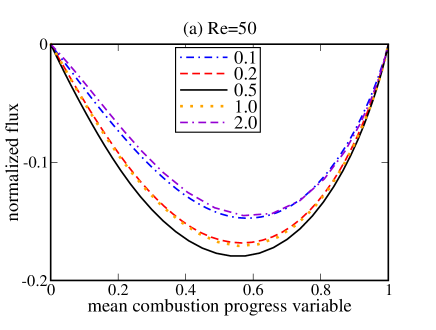
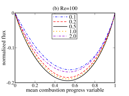
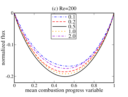
Figure 2: Dependencies of the normalized turbulent scalar flux $\overline{u^{\prime}c^{\prime}}/u_{0}$ on the mean reaction progress variable $\overline{c}$, computed at different ratios of $S_{{}_{L}}/u_{0}$ specified in legends for (a) ${\rm Re}=50$, (b) ${\rm Re}=100$, and (c) ${\rm Re}=200$.

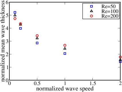
Figure 3: Dependencies of the normalized mean turbulent wave thickness $\delta_{\rm t}/\ell_{11}$ on the normalized wave speed $S_{{}_{L}}/u_{0}$ computed at three different turbulent Reynolds numbers, ${\rm Re}$, specified in legends.

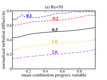
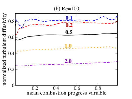
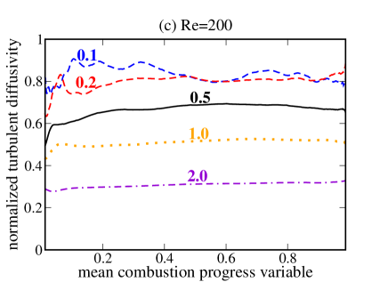
Figure 4: Dependencies of the normalized turbulent scalar diffusivity $D_{T}/(u_{0}\ell_{11})$ on the mean reaction progress variable $\overline{c}$, computed for (a) ${\rm Re}=50$, (b) ${\rm Re}=100$, and (c) ${\rm Re}=200$. Values of $S_{{}_{L}}/u_{0}$ are specified near curves.

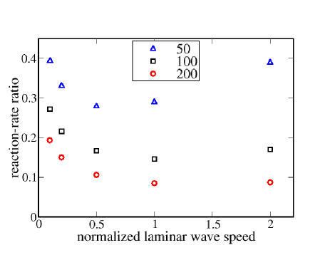
Figure 5: Reaction-rate ratio $\theta={\rm max}\{\overline{W}(\overline{c})\}/{\rm max}\{W(c)\}$ vs. $S_{L}/u_{0}$. Symbols show DNS data, with the Reynolds numbers Re being specified in legends.

Figure 2 shows dependencies of the normalized turbulent scalar flux $\overline{u^{\prime}c^{\prime}}/u_{0}$ versus the mean reaction progress variable $\overline{c}$, computed for (a) ${\rm Re}=50$, (b) ${\rm Re}=100$, and (c) ${\rm Re}=200$. In unburnt or burnt mixture, the instantaneous progress variable is constant, $c=0$ or $c=1$, respectively. This implies that in the two regions turbulent flux $\overline{c^{\prime}{\bm{u}}^{\prime}}=0$. Inside the mean reaction wave the mean progress variable $\overline{c}$ varies between 0 and 1. In this region the gradient ${\bm{\nabla}}\overline{c}$ does not vanish. Since ${\bm{\nabla}}\overline{c}$ is positive in this region (in the coordinate framework used in the paper), the turbulent flux $\overline{c^{\prime}{\bm{u}}^{\prime}}=-D_{T}{\bm{\nabla}}\overline{c}$ is negative inside the mean reaction wave. The absolute value of the turbulent flux $|\overline{c^{\prime}{\bm{u}}^{\prime}}|$ reaches maximum at the point where the gradient ${\bm{\nabla}}\overline{c}$ is maximum. If the probability of deviation of the reaction wave from its mean position is described by the Gaussian distribution, the gradient ${\bm{\nabla}}\overline{c}$ is maximum at $\overline{c}=0.5$. For instance, in various premixed turbulent flames, ${\bm{\nabla}}\overline{c}$ does peak at $\overline{c}=0.5$, e.g. see Fig. 4.22 and Eqs. (4.34) and (4.35) in CRC . While, the flux magnitude depends on $S_{{}_{L}}/u_{0}$ and, hence, on ${\rm Da}_{{}_{\rm DNS}}$, see Table I, such variations in the flux magnitude are sufficiently weak and non-monotonic, with the peak magnitude being obtained at a medium $S_{{}_{L}}/u_{0}=0.5$.

On the contrary, the mean turbulent wave thickness $\delta_{\rm t}$ defined using the maximum gradient method, i.e.,

$$\delta_{\rm t}=\frac{1}{\max{\{\nabla_{x}\overline{c}\}}},$$ (19)

decreases rapidly with the increase of the normalized wave speed $S_{{}_{L}}/u_{0}$ and, hence, ${\rm Da}_{{}_{\rm DNS}}$, see Fig. 3. This numerical result is fully consistent with the theory, which predicts a decrease in $D_{T}$ with increasing Damköhler number. Under the DNS conditions, an increase in $S_{L}/u_{0}$ results in increasing ${\rm Da}$ and, therefore, decreasing $D_{T}$. Consequently, $\delta_{\rm t}\propto\left[D_{T}({\rm Da})\,\tau_{c}\right]^{1/2}$ decreases with increasing $S_{L}/u_{0}$.

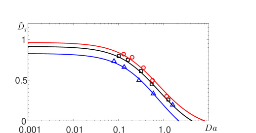
Figure 6: Theoretical dependence $\tilde{D}_{T}\equiv D_{T}/D^{T}_{0}$ versus Damköhler number ${\rm Da}$ determined by Eq. (12) for different values of the Reynolds number ${\rm Re}=$ 50 (blue), 100 (black), 200 (red) at ${\rm Pr}=1$. The DNS data on $\langle D_{T}\rangle$ normalized using $u_{0}l_{11}$ are shown in blue triangles (${\rm Re}=$ 50), black squares (${\rm Re}=$ 100), and red circles (${\rm Re}=$ 200).

Accordingly, the gradient of the mean reaction progress variable is increased by $S_{{}_{L}}/u_{0}$ (or ${\rm Da}_{{}_{\rm DNS}}$), whereas turbulent diffusivity evaluated as follows,

$$D_{T}(\overline{c})=-\frac{\overline{u^{\prime}c^{\prime}}}{\nabla_{x}\overline{c}},$$ (20)

is decreased with increasing $S_{{}_{L}}/u_{0}$ and ${\rm Da}_{{}_{\rm DNS}}$, see Fig. 4. The decrease of the turbulent diffusion coefficient, $D_{T}$, with the increase of the Damköhler number observed in DNS, agrees well with the developed theory.

Moreover, Fig. 4 indicates that $D_{T}$ evaluated using Eq. (20) depends weakly on $\overline{c}$, thus, implying that the influence of the reaction on the turbulent diffusion coefficient may be characterized with a single mean turbulent diffusivity defined as follows

$$\overline{\langle D_{T}\rangle}=\int_{0}^{1}D_{T}(\xi)d\xi.$$ (21)

To compare values of the mean turbulent diffusion coefficient, $\overline{\langle D_{T}\rangle}$, obtained in the simulations with the theoretical predictions for $D_{T}({\rm Da})$ we need to take into account that the Damköhler number, ${\rm Da}_{{}_{\rm DNS}}$, used in DNS is different from the Damköhler number, ${\rm Da}$, used in the theory. In the DNS, due to strong fluctuations in the scalar field $c$ and, especially, $W(c)$, the mean reaction rate is characterized by a significantly larger chemical time scale $\overline{\tau_{c}}$ when compared to the time scale $\tau_{F}$ associated with the laminar $W(c)$. A ratio of these two time scales $\theta=\tau_{F}/\overline{\tau_{c}}={\rm Da}/{\rm Da}_{{}_{\rm DNS}}$ can be estimated as $\theta={\rm max}\{\overline{W}(\overline{c})\}/{\rm max}\{W(c)\}$. The reaction-rate ratio $\theta$ versus $S_{L}/u_{0}$ is shown in Fig. 4 for different values of the Reynolds number Re.

Using the values of $\theta$ obtained in the DNS and plotted in Fig. 4, we relate the Damköhler number, ${\rm Da}$, used in the theory with ${\rm Da}_{{}_{\rm DNS}}$, used in DNS: ${\rm Da}=\theta\,{\rm Da}_{{}_{\rm DNS}}$. In Fig. 6 the mean turbulent diffusion coefficient, $\overline{\langle D_{T}\rangle}$, versus ${\rm Da}=\theta\,{\rm Da}_{{}_{\rm DNS}}$ obtained in the simulations (symbols) is compared with the theoretical predictions for $D_{T}$ given by Eq. (12). Figure 6 demonstrates very good agreement between results of DNS and theoretical predictions.

V Conclusion

The theory of turbulent diffusion in reacting flows previously developed in EKR98 ; EKLR14 , has been generalized for finite Reynolds numbers and the dependence of turbulent diffusion coefficient versus two parameters, the Reynolds number and Damköhler number has been obtained. Validation of the generalized theory of the effect of chemical reaction on turbulent diffusion using three-dimensional DNS of a finite thickness reaction wave propagation in forced, homogeneous, isotropic, and incompressible turbulence for the first-order chemical reactions, has revealed a very good quantitative agreement between the theoretical predictions and the DNS results.

- (1) G. T. Csanady, Turbulent Diffusion in the Environment (Reidel, Dordrecht, 1980).
- (2) A. K. Blackadar, Turbulence and Diffusion in the Atmosphere (Springer, Berlin, 1997).
- (3) R. O. Fox, Computational Models for Turbulent Reacting Flows (Cambridge University Press, NY, 2003).
- (4) N. Peters, Turbulent Combustion (Cambridge Univ. Press, Cambridge, 2004).
- (5) J. H. Seinfeld and S. N. Pandis, Atmospheric Chemistry and Physics. From Air Pollution to Climate Change, 2nd ed. (John Wiley & Sons, NY, 2006).
- (6) L. I. Zaichik, V. M. Alipchenkov, and E. G. Sinaiski, Particles in Turbulent Flows (John Wiley & Sons, NY, 2008).
- (7) M. Liberman, Introduction to Physics and Chemistry of Combustion (Springer-Verlag, NY, 2008).
- (8) A. N. Lipatnikov, Fundamentals of Premixed Turbulent Combustion (CRC Press, Boca Raton, 2012).
- (9) P. A. Libby, Prog. Energy Combust. Sci. 11, 83 (1985).
- (10) K. N. C. Bray, Proc. R. Soc. London A451, 231 (1995).
- (11) A. N. Lipatnikov and J. Chomiak, Prog. Energy Combust. Sci. 36, 1 (2010).
- (12) N. Swaminathan and K. N. C. Bray, Turbulent Premixed Flames (Cambridge Univ. Press, Cambridge, 2011).
- (13) V. A. Sabelnikov and A. N. Lipatnikov, Annu. Rev. Fluid Mech. 49, 91 (2017).
- (14) V. A. Sabelnikov and A. N. Lipatnikov, Combust. Theory Modelling 17, 1154 (2013).
- (15) V. A. Sabelnikov and A. N. Lipatnikov, Phys. Rev. E 90, 033004 (2014).
- (16) V. A. Sabelnikov and A. N. Lipatnikov, Combust. Flame 162, 2893 (2015).
- (17) S. Corrsin, Adv. Geophysics 18A, 25 (1974).
- (18) R. Borghi and D. Dutoya, Proc. Combust. Inst. 17, 235 (1978).
- (19) A. N. Lipatnikov, Proc. Combust. Inst. 33, 1497 (2011).
- (20) T. Elperin, N. Kleeorin, and I. Rogachevskii, Phys. Rev. Lett. 80, 69 (1998).
- (21) T. Elperin, N. Kleeorin, M. A. Liberman, and I. Rogachevskii, Phys. Rev. E 90, 053001 (2014).
- (22) A. Brandenburg, N. E. L. Haugen, and N. Babkovskaia, Phys. Rev. E 83, 016304 (2011).
- (23) A. N. Kolmogorov, I. G. Petrovskii, and N. S. Piskunov, Moscow Univ. Bull. Math. 1, 1 (1937).
- (24) R. A. Fisher, Ann. Eugenics 7, 353 (1937).
- (25) S. A. Orszag, J. Fluid Mech. 41, 363 (1970).
- (26) A. S. Monin and A. M. Yaglom, Statistical Fluid Mechanics (MIT Press, Cambridge, Massachusetts, 1975), Vol. 2.
- (27) W. D. McComb, The Physics of Fluid Turbulence (Clarendon, Oxford, 1990).
- (28) A. Pouquet, U. Frisch, and J. Leorat, J. Fluid Mech. 77, 321 (1976).
- (29) A. Brandenburg and K. Subramanian, Phys. Rept. 417, 1 (2005).
- (30) I. Rogachevskii and N. Kleeorin, Phys. Rev. E 76, 056307 (2007).
- (31) I. Rogachevskii,N. Kleeorin, P. J. Käpylä, A. Brandenburg, Phys. Rev. E 84, 056314 (2011).
- (32) G. K. Batchelor, The Theory of Homogeneous Turbulence (Cambridge Univ. Press, New York, 1953).
- (33) R. Yu, J. Yu, and X.-S. Bai, J. Comp. Phys. 231, 5504 (2012).
- (34) R. Yu, A. N. Lipatnikov, and X.-S. Bai, Phys. Fluids 26, 085104 (2014).
- (35) R. Yu, X.-S. Bai, and A. N. Lipatnikov, J. Fluid Mech. 772, 127 (2015).
- (36) R. Yu and X.-S. Bai, J. Comp. Phys. 256, 234 (2014).
- (37) R. Yu and A. N. Lipatnikov, Phys. Rev. E 95, 063101 (2017).
- (38) R. Yu and A. N. Lipatnikov, Phys. Fluids 29, 065116 (2017).
- (39) S. Ghosal, T. S. Lund, P. Moin, and K. Akselvoll, J. Fluid Mech. 286, 229 (1995).
- (40) R. Yu, X.-S. Bai, and V. Bychkov, Phys. Rev. E 92, 063028 (2015).
- (41) L. D. Landau and E. M. Lifshitz, Fluid Mechanics, 2nd ed. (Elsevier, Oxford, 2009).