11institutetext: G. Boué 22institutetext: 22email: gwenael.boue@obspm.fr IMCCE, Observatoire de Paris, UPMC Univ. Paris 6, Paris, France

The Two Rigid Body Interaction using Angular Momentum Theory Formulae

Gwenaël Boué
(Received: date / Accepted: date)
Abstract

This work presents an elegant formalism to model the evolution of the full two rigid body problem. The equations of motion, given in a Cartesian coordinate system, are expressed in terms of spherical harmonics and Wigner D-matrices. The algorithm benefits from the numerous recurrence relations satisfied by these functions allowing a fast evaluation of the mutual potential. Moreover, forces and torques are straightforwardly obtained by application of ladder operators taken from the angular momentum theory and commonly used in quantum mechanics. A numerical implementation of this algorithm is made. Tests show that the present code is significantly faster than those currently available in literature.

Keywords:
full two rigid problem binary systems spin-orbit coupling numerical method

1 Introduction

Modelling the evolution of two rigid bodies with arbitrary shapes in gravitational interaction is not an easy task. The first obstacle is the determination of the mutual potential, the second is the derivation of the equations of motion in a suitable form to allow fast computation. In general cases, the potential has to be expanded and truncated at some order in the ratio of the bodies mean radii to the distance between the two barycenters. Using the angular momentum theory developed by Wigner (1959), Borderies (1978) manage to provide a compact expression of the mutual potential at any order. In this expression, the gravity field of each body is described by Stokes coefficients, the relative orientation of the two bodies appears through Wigner D-matrices – also called Euler functions (Borderies, 1978) – and the dependence in the distance between the two barycenters is embedded in solid harmonics. Equations of motion associated to this expansion have been proposed by Maciejewski (1995). A strictly equivalent formalism based on symmetric trace-free (STF) tensor (Hartmann et al, 1994; Mathis and Le Poncin-Lafitte, 2009) has been implemented by Compère and Lemaître (2014) who studied numerically the evolution of the binary asteroid 1999 KW4.

The decomposition in spherical harmonics has sometimes been discarded based on the misconception that this formalism involves many trigonometric functions increasing as much the computation time and the risk of numerical instabilities. To circumvent this issue, alternative decompositions of the potential have been applied. For instance, Paul (1988) explicitly wrote the mutual potential in Cartesian coordinates at all orders. The associated equations of motion were then provided by Tricarico (2008). Recently, Hou et al (2016) (hereafter, HSX16) revisited this approach and built the as yet fastest algorithm able to integrate the full two rigid body problem thanks to a set of recurrence formulae whose coefficients can be computed and stored beforehand. Another example of alternative is the so-called polyhedron approach relying on Stokes’ theorem in which the volume integral leading to the mutual potential is converted into a surface integral over the boundaries of the two bodies (Werner and Scheeres, 2005). This algorithm implemented by Fahnestock and Scheeres (2006) was at the time the fastest integrator.

Here we revisit Borderies’ expression of the mutual potential developed in spherical harmonics, but we express them in Cartesian coordinates. By consequence, the description of the orbital configuration is actually equivalent to those where the potential is explicitly written in Cartesian coordinates as in (Paul, 1988), for instance. The main contribution of the present study is in the parametrisation of rotations. Whereas in previous works, torques are computed by an explicit derivation of the potential energy with respect to Euler angles or with respect to rotation matrix elements, here forces and torques are simply obtained by application of ladder operators taken from quantum mechanics theory. This approach has already been successfully applied to the modelling of tidal evolution of close-in planets (Boué et al, 2016). In this study we show that it allows to built the fastest numerical integrator of the full two rigid body problem.

The paper is organised as follows: in Section 2, the equations of motion are computed using Poincaré’s method (Poincaré, 1901). Forces and torques are written in terms of ladder operators commonly used in quantum mechanics. The section also contains all the recurrence relations allowing an efficient numerical implementation of the problem. Numerical tests are performed in Section 3. Conclusions are drawn in the last section.

2 Equations of motion

Let two rigid bodies $A$ and $B$ with arbitrary shapes in gravitational interaction in an inertial frame $(O;\vec{e}_{x},\vec{e}_{y},\vec{e}_{z})$. For both bodies $A$ and $B$ we define body-fixed frames centred on their respective barycenters $O_{A}$ and $O_{B}$ which are $(O_{A};\vec{e}^{A}_{x},\vec{e}^{A}_{y},\vec{e}^{A}_{z})$ and $(O_{B};\vec{e}^{B}_{x},\vec{e}^{B}_{y},\vec{e}^{B}_{z})$, respectively. To fasten the integration, the problem is not described in the inertial frame as in (Borderies, 1978), but in the body-fixed frame of $A$ (Maciejewski, 1995). This is also the choice of HSX16 with whom we wish to compare the method. The convention used in this paper is the following: unprimed quantities are expressed in the body-fixed frame of $A$, while primed ones are written in the body-fixed frame of $B$. Vectors expressed in the inertial frame are written with the superscript 00.

2.1 Lagrangian

Following Maciejewski (1995), the potential reads

$$\begin{split}U_{AB}=&-GM_{A}M_{B}\sum_{l_{1}=0}^{\infty}\sum_{m_{1}=-l_{1}}^{l_{1}}\sum_{l_{2}=0}^{\infty}\sum_{m_{2}=-l_{2}}^{l_{2}}\bigg{(}R_{A}^{l_{1}}R_{B}^{l_{2}}Z_{l_{1},m_{1}}^{A}Z^{B}_{l_{2},m_{2}}\\ &\times(-1)^{l_{2}}\gamma^{l_{1},m_{1}}_{l_{2},m_{2}}\frac{Y_{l_{1}+l_{2},m_{1}+m_{2}}(\vec{r})}{r^{l_{1}+l_{2}+1}}\bigg{)}\end{split}$$ (1)

where $M_{*}$, $R_{*}$, and $Z^{*}_{l,m}$ are the mass, the mean radius and Stokes coefficients of the body $*=A,B$, respectively. Note that $Z^{A}_{l,m}$ is constant while $Z^{B}_{l,m}$ is not because both quantities are written in the body-fixed frame of $A$. The radius vector $\vec{r}=\vec{r}_{B}-\vec{r}_{A}$ connects the two barycenters. $Y_{l,m}$ are complex spherical harmonics and $\gamma^{l_{1},m_{1}}_{l_{2},m_{2}}$ are constant coefficients. Here we use the Schmidt semi-normalisation of the spherical harmonics, such that,

$$Y_{l,m}(\theta,\phi)=(-1)^{m}\sqrt{\frac{(l-m)!}{(l+m)!}}P_{l,m}(\cos\theta)\mathrm{e}^{\mathrm{i}m\phi}$$ (2)

where the associated Legendre polynomials $P_{l,m}$ are defined as

$$P_{l,m}(x)=\frac{1}{2^{l}l!}(1-x^{2})^{m/2}\frac{\mathrm{d}^{l+m}}{\mathrm{d}x^{l+m}}(x^{2}-1)^{l}.$$

The complex Stokes coefficients $Z_{l,m}$ are related to the usual real Stokes coefficients $C_{l,m}$ and $S_{l,m}$ by

$$Z_{l,m}=(-1)^{m}\frac{1+\delta_{m,0}}{2}\sqrt{\frac{(l+m)!}{(l-m)!}}(C_{l,m}-\mathrm{i}S_{l,m})\ ,\quad\mathrm{for}\quad m\geq 0$$ (3a)
and the symmetry relation
$$Z_{l,m}=(-1)^{m}{\bar{Z}}_{l,-m}\ ,\quad\mathrm{for}\quad m<0\ .$$ (3b)

In Eq. (3a), $\delta_{i,j}$ is the Kronecker delta equal to 1 if $i=j$ and equal to 0 otherwise. In Eq. (3b), the bar above $Z_{l,m}$ denotes the complex conjugate. Following our normalisation convention, the coefficients $\gamma^{l_{1},m_{1}}_{l_{2},m_{2}}$ are

$$\gamma^{l_{1},m_{1}}_{l_{2},m_{2}}=\sqrt{\frac{(l_{1}+l_{2}-m_{1}-m_{2})!(l_{1}+l_{2}+m_{1}+m_{2})!}{(l_{1}+m_{1})!(l_{1}-m_{1})!(l_{2}+m_{2})!(l_{2}-m_{2})!}}.$$

Let

$$\vec{C}_{A}=[\vec{e}^{A}_{x},\vec{e}^{A}_{y},\vec{e}^{A}_{z}],\qquad\vec{C}_{B}=[\vec{e}^{B}_{x},\vec{e}^{B}_{y},\vec{e}^{B}_{z}]\qquad\mathrm{and}\qquad\vec{C}={\vec{C}}^{T}_{A}\vec{C}_{B}$$

be the rotation matrices such that

$$\vec{r}={\vec{C}}^{T}_{A}\vec{r}^{0},\qquad Z^{B}_{l,m}=\sum_{m^{\prime}=-l}^{l}D^{l}_{m,m^{\prime}}(\vec{C})Z^{\prime B}_{l,m^{\prime}}\ ,$$

where ${\vec{C}}^{T}_{A}$ means the transpose of $\vec{C}_{A}$ and $D^{l}_{m,m^{\prime}}(\vec{C})$ is an element of Wigner D-matrix associated to the rotation $\vec{C}$. $Z^{\prime B}_{l,m^{\prime}}$ are the (constant) complex Stokes coefficients of body $B$ expressed in its body-fixed frame.

In the barycentric frame, the kinetic energy of the system reads

$$T=\frac{1}{2}{\vec{\Omega}}^{T}_{A}\vec{I}_{A}\vec{\Omega}_{A}+\frac{1}{2}{(\vec{\Omega}+\vec{\Omega}_{A})}^{T}\vec{I}_{B}(\vec{\Omega}+\vec{\Omega}_{A})+\frac{1}{2}\mu\|\vec{v}+\vec{\Omega}_{A}\times\vec{r}\|^{2}$$ (4)

where $\vec{I}_{A}$ and $\vec{I}_{B}$ are the inertia matrices of the bodies $A$ and $B$ expressed in the the body-fixed frame of $A$, respectively. $\vec{\Omega}_{A}$ is the rotation vector of the body $A$ with respect to the inertial frame, while $\vec{\Omega}=\vec{\Omega}_{B}-\vec{\Omega}_{A}$ is the rotation vector of the body $B$ relative to the body $A$. $\mu=M_{A}M_{B}/(M_{A}+M_{B})$ is the reduced mass and $\vec{v}=\dot{\vec{r}}$ is the relative velocity in the body-fixed frame of $A$. In the expression of the kinetic energy (Eq. 4), $\vec{I}_{A}$ is constant while $\vec{I}_{B}=\vec{C}\vec{I}^{\prime}_{B}{\vec{C}}^{T}$ is a function of $\vec{C}$.

The Lagrangian of the problem $f=T-U_{AB}$ is a function of $\vec{q}=(\vec{C}_{A},\vec{C},\vec{r})$ and $\vec{\eta}=(\vec{\Omega}_{A},\vec{\Omega},\vec{v})$. Note that $\vec{C}_{A}$ and $\vec{C}$ are themselves functions of only three coordinates, such as the 3-2-3 Euler angles $(\alpha_{A},\beta_{A},\gamma_{A})$ and $(\alpha,\beta,\gamma)$, respectively:

$$\vec{C}_{A}(\alpha_{A},\beta_{A},\gamma_{A})=\vec{C}_{z}(\alpha_{A})\vec{C}_{y}(\beta_{A})\vec{C}_{z}(\gamma_{A}),\qquad\vec{C}(\alpha,\beta,\gamma)=\vec{C}_{z}(\alpha)\vec{C}_{y}(\beta)\vec{C}_{z}(\gamma).$$

To retrieve the equations of motion given by Maciejewski (1995), we use Poincaré’s forme nouvelle des équations de la mécanique (Poincaré, 1901). We define a vector field basis associated to infinitesimal rotations of the body $A$ as

$\displaystyle\hat{\cal{J}}_{A,x}$ $\displaystyle=$ $\displaystyle\cos\gamma_{A}\cot\beta_{A}\frac{\partial}{\partial\gamma_{A}}+\sin\gamma_{A}\frac{\partial}{\partial\beta_{A}}-\frac{\cos\gamma_{A}}{\sin\beta_{A}}\frac{\partial}{\partial\alpha_{A}},$ (5a)
$\displaystyle\hat{\cal{J}}_{A,y}$ $\displaystyle=$ $\displaystyle-\sin\gamma_{A}\cot\beta_{A}\frac{\partial}{\partial\gamma_{A}}+\cos\gamma_{A}\frac{\partial}{\partial\beta_{A}}+\frac{\sin\gamma_{A}}{\sin\beta_{A}}\frac{\partial}{\partial\alpha_{A}},$ (5b)
$\displaystyle\hat{\cal{J}}_{A,z}$ $\displaystyle=$ $\displaystyle\frac{\partial}{\partial\gamma_{A}}.$ (5c)

Equivalently, we introduce a basis field corresponding to infinitesimal rotations of the body $B$ relative to the body $A$:

$\displaystyle\hat{\cal{J}}_{x}$ $\displaystyle=$ $\displaystyle-\cos\alpha\cot\beta\frac{\partial}{\partial\alpha}-\sin\alpha\frac{\partial}{\partial\beta}+\frac{\cos\alpha}{\sin\beta}\frac{\partial}{\partial\gamma},$ (6a)
$\displaystyle\hat{\cal{J}}_{y}$ $\displaystyle=$ $\displaystyle-\sin\alpha\cot\beta\frac{\partial}{\partial\alpha}+\cos\alpha\frac{\partial}{\partial\beta}+\frac{\sin\alpha}{\sin\beta}\frac{\partial}{\partial\gamma},$ (6b)
$\displaystyle\hat{\cal{J}}_{z}$ $\displaystyle=$ $\displaystyle\frac{\partial}{\partial\alpha}.$ (6c)

At last, we consider the canonical vector field basis associated to infinitesimal translations

$\displaystyle\hat{\cal{P}}_{x}$ $\displaystyle=$ $\displaystyle\frac{\partial}{\partial x},$ (7a)
$\displaystyle\hat{\cal{P}}_{y}$ $\displaystyle=$ $\displaystyle\frac{\partial}{\partial y},$ (7b)
$\displaystyle\hat{\cal{P}}_{z}$ $\displaystyle=$ $\displaystyle\frac{\partial}{\partial z}.$ (7c)

Let us gather all these vector fields into a single vector $\hat{\vec{\cal{X}}}=(\hat{\vec{\cal{J}}}_{A},\hat{\vec{\cal{J}}},\hat{\vec{\cal{P}}})$. The generalised velocity vector $\dot{\vec{q}}$ of the Lagrangian reads

$$\dot{\vec{q}}=\vec{\eta}\cdot\hat{\vec{\cal{X}}}(\vec{q})\equiv\sum_{i=1}^{9}\eta_{i}\hat{\cal{X}}_{i}(\vec{q}),$$ (8)

as required by Poincaré’s formalism. The equations of motion of $\vec{C}_{A}$, $\vec{C}$, and $\vec{r}$ given by Eq. (8) are made explicit in the following. To obtain the equations of motion, we need the structure constants $c_{ij}^{k}$ defined as

$$[\hat{\cal{X}}_{i},\hat{\cal{X}}_{j}]\equiv\hat{\cal{X}}_{i}\hat{\cal{X}}_{j}-\hat{\cal{X}}_{j}\hat{\cal{X}}_{i}=c_{ij}^{k}\hat{\cal{X}}_{k}.$$

A direct calculation shows that the non-vanishing commutators are

$$\begin{array}[]{ll}&[\hat{\cal{J}}_{A,x},\hat{\cal{J}}_{A,y}]=-\hat{\cal{J}}_{A,z},\\[5.0pt] &[\hat{\cal{J}}_{A,y},\hat{\cal{J}}_{A,z}]=-\hat{\cal{J}}_{A,x},\\[5.0pt] &[\hat{\cal{J}}_{A,z},\hat{\cal{J}}_{A,x}]=-\hat{\cal{J}}_{A,y},\end{array}\qquad\begin{array}[]{ll}&[\hat{\cal{J}}_{x},\hat{\cal{J}}_{y}]=\hat{\cal{J}}_{z},\\[5.0pt] &[\hat{\cal{J}}_{y},\hat{\cal{J}}_{z}]=\hat{\cal{J}}_{x},\\[5.0pt] &[\hat{\cal{J}}_{z},\hat{\cal{J}}_{x}]=\hat{\cal{J}}_{y}.\end{array}$$ (9)

To get Poincaré’s equation, we also need to evaluate $\hat{\cal{X}}_{i}(f)$. We have

$\displaystyle\hat{\vec{\cal{J}}}_{A}(f)$ $\displaystyle=$ $\displaystyle\vec{0},$ (10a)
$\displaystyle\hat{\vec{\cal{J}}}(f)$ $\displaystyle=$ $\displaystyle\vec{G}_{B}\times(\vec{\Omega}+\vec{\Omega}_{A})-\hat{\vec{\cal{J}}}(U_{AB}),$ (10b)
$\displaystyle\hat{\vec{\cal{P}}}(f)$ $\displaystyle=$ $\displaystyle\mu\vec{V}\times\vec{\Omega}_{A}-\hat{\vec{\cal{P}}}(U_{AB}).$ (10c)

The equation (10a) results from the invariance by rotation of the problem. Indeed, the Lagrangian does not depend on $\vec{C}_{A}$. In Eq. (10c), $\vec{V}=\vec{v}+\vec{\Omega}_{A}\times\vec{r}$ represents the velocity relative to the barycentric frame expressed in the body-fixed frame of $A$. In Eq. (10b), we have introduce $\vec{G}_{B}=\vec{I}_{B}(\vec{\Omega}+\vec{\Omega}_{A})$, the angular momentum of the body $B$. Similarly, we denote by $\vec{G}_{A}=\vec{I}_{A}\vec{\Omega}_{A}$ the angular momentum of the body $A$, and by $\vec{L}=\mu\vec{r}\times\vec{V}$, the orbital angular momentum. The last ingredients in Poincaré’s equations are the partial derivatives of the kinetic energy with respect to $\vec{\eta}$ which are

$$\frac{\partial T}{\partial\vec{\Omega}_{A}}=\vec{G}_{A}+\vec{G}_{B}+\vec{L},\qquad\frac{\partial T}{\partial\vec{\Omega}}=\vec{G}_{B},\qquad\frac{\partial T}{\partial\vec{v}}=\mu\vec{V}.$$ (11)

Combining Eqs. (8), (9), (10), (11), and Poincaré’s equations

$$\frac{d}{dt}\frac{\partial T}{\partial\eta_{i}}=\sum_{j,k}c_{ij}^{k}\eta_{j}\frac{\partial T}{\partial\eta_{k}}+\hat{\cal{X}}_{i}(f),$$

we get

$$\left\{\begin{array}[]{ll}\dot{\vec{C}}_{A}=\vec{\Omega}_{A}\cdot\hat{\vec{\cal{J}}}_{A}(\vec{C}_{A}),\\[5.0pt] \dot{\vec{C}}=(\vec{\Omega}_{B}-\vec{\Omega}_{A})\cdot\hat{\vec{\cal{J}}}(\vec{C}),\\[5.0pt] \dot{\vec{r}}=\vec{r}\times\vec{\Omega}_{A}+\vec{V},\end{array}\right.\qquad\left\{\begin{array}[]{ll}\dot{\vec{G}}_{A}=\vec{G}_{A}\times\vec{\Omega}_{A}+\vec{T}_{A},\\[5.0pt] \dot{\vec{G}}_{B}=\vec{G}_{B}\times\vec{\Omega}_{A}+\vec{T}_{B},\\[5.0pt] \dot{\vec{V}}=\vec{V}\times\vec{\Omega}_{A}+\frac{1}{\mu}\vec{F},\end{array}\right.$$ (12)

with

$$\vec{F}=-\hat{\vec{\cal{P}}}(U_{AB}),\qquad\vec{T}=-\hat{\vec{\cal{L}}}(U_{AB}),\qquad\vec{T}_{B}=-\hat{\vec{\cal{J}}}(U_{AB}),\qquad\vec{T}_{A}=-\vec{T}-\vec{T}_{B}.$$

The rotation vectors are given by

$$\vec{\Omega}_{A}=\vec{I}_{A}^{-1}\vec{G}_{A},\qquad\vec{\Omega}_{B}=\vec{I}^{-1}_{B}\vec{G}_{B},$$

and the vector field $\hat{\vec{\cal{L}}}$ is defined as

$\displaystyle\hat{\cal{L}}_{x}$ $\displaystyle=$ $\displaystyle y\frac{\partial}{\partial z}-z\frac{\partial}{\partial y},$ (13a)
$\displaystyle\hat{\cal{L}}_{y}$ $\displaystyle=$ $\displaystyle z\frac{\partial}{\partial x}-x\frac{\partial}{\partial z},$ (13b)
$\displaystyle\hat{\cal{L}}_{z}$ $\displaystyle=$ $\displaystyle x\frac{\partial}{\partial y}-y\frac{\partial}{\partial x}.$ (13c)

The equations (12) are strictly equivalent to Maciejewski’s equations of motion, but they are explicitly written in terms of the vector fields $\hat{\vec{\cal{P}}}$, $\hat{\vec{\cal{L}}}$, $\hat{\vec{\cal{J}}}_{A}$ and $\hat{\vec{\cal{J}}}$. As shown in the subsequent section, textbooks on quantum theory of angular momentum allow to evaluate these vector fields applied to $U_{AB}$ very efficiently.

2.2 Ladder operators, force and torques

We introduce a complex coordinate system $(\vec{e}_{+},\vec{e}_{0},\vec{e}_{-})$ in which coordinates of any vector $\vec{a}$ are denoted $(a_{+},a_{0},a_{-})$ and are related to the usual Cartesian coordinates $(a_{x},a_{y},a_{z})$ by

$$a_{+}=-\frac{1}{\sqrt{2}}(a_{x}+\mathrm{i}a_{y})\qquad a_{0}=a_{z}\qquad a_{-}=\frac{1}{\sqrt{2}}(a_{x}-\mathrm{i}a_{y})\ .$$

We apply the same rule for vector fields $\hat{\vec{\cal{A}}}=(\hat{\cal{A}}_{x},\hat{\cal{A}}_{y},\hat{\cal{A}}_{z})$. We get

$$\hat{\cal{A}}_{+}=-\frac{1}{\sqrt{2}}(\hat{\cal{A}}_{x}+\mathrm{i}\hat{\cal{A}}_{y})\qquad\hat{\cal{A}}_{0}=\hat{\cal{A}}_{z}\qquad\hat{\cal{A}}_{-}=\frac{1}{\sqrt{2}}(\hat{\cal{A}}_{x}-\mathrm{i}\hat{\cal{A}}_{y}).$$

The vector fields defined in Eqs. (5), (6), (7), and (13) are related to ladder operators commonly used in quantum theory of angular momentum. With the notation of Varshalovich et al (1988), we have

$$\hat{\cal{J}}_{A,\nu}\equiv\mathrm{i}\hat{J}^{\prime\nu}(\alpha_{A},\beta_{A},\gamma_{A}),\qquad\hat{\cal{J}}_{\nu}\equiv\mathrm{i}\hat{J}_{\nu}(\alpha,\beta,\gamma),\qquad\hat{\cal{P}}_{\nu}\equiv\nabla_{\nu},\qquad\hat{\cal{L}}_{\nu}\equiv\mathrm{i}\hat{L}_{\nu},$$

for $\nu\in\{+,0,-\}$. $\hat{J}^{\prime\nu}$ and $\hat{J}_{\nu}$ are the components of the spin operator expressed in the rotated frame and in the initial frame, respectively. $\nabla_{\nu}$ is the usual gradient operator and $\hat{L}_{\nu}$ is the orbital angular momentum operator. Given these equivalences, we deduce the following relations (Varshalovich et al, 1988)

$$\hat{\cal{P}}_{\nu}\left(\frac{Y_{l,m}(\vec{r})}{r^{l+1}}\right)=\left\{\begin{array}[]{ll}\displaystyle-\sqrt{(l+m+1)(l-m+1)}\frac{Y_{l+1,m}(\vec{r})}{r^{l+2}}&\nu=0\\[5.0pt] \displaystyle-\sqrt{\frac{(l\pm m+1)(l\pm m+2)}{2}}\frac{Y_{l+1,m\pm 1}(\vec{r})}{r^{l+2}}&\nu=\pm 1\end{array}\right.$$ (14a)
and
$$\hat{\cal{L}}_{\nu}\left(\frac{Y_{l,m}(\vec{r})}{r^{l+1}}\right)=\mathrm{i}\left\{\begin{array}[]{ll}\displaystyle m\frac{Y_{l,m}(\vec{r})}{r^{l+1}}&\nu=0\\ \displaystyle\mp\sqrt{\frac{l(l+1)-m(m\pm 1)}{2}}\frac{Y_{l,m\pm 1}(\vec{r})}{r^{l+1}}&\nu=\pm 1\end{array}\right.\ ,$$ (14b)

for the orbital part (embedded in the spherical harmonics), while spin operators act on Wigner D-matrices according to

$$\hat{\cal{J}}_{\nu}D^{l}_{m,m^{\prime}}(\vec{C})=\mathrm{i}\left\{\begin{array}[]{ll}-mD^{l}_{m,m^{\prime}}(\vec{C})\ ,&\nu=0,\\[5.0pt] \pm\sqrt{\displaystyle\frac{l(l+1)-m(m\mp 1)}{2}}D^{l}_{m\mp 1,m^{\prime}}(\vec{C})&\nu=\pm 1\end{array}\right.$$ (15a)
and
$$\hat{\cal{J}}_{A,\nu}D^{l}_{m,m^{\prime}}(\vec{C}_{A})=\mathrm{i}\left\{\begin{array}[]{ll}-m^{\prime}D^{l}_{m,m^{\prime}}(\vec{C}_{A})\ ,&\nu=0,\\[5.0pt] \pm\sqrt{\displaystyle\frac{l(l+1)-m^{\prime}(m^{\prime}\pm 1)}{2}}D^{l}_{m,m^{\prime}\pm 1}(\vec{C}_{A})&\nu=\pm 1\end{array}\right.\ .$$ (15b)

Forces and torques are then computed as follows. Let us define the constant terms $u^{l_{1},m_{1}}_{l_{2},m_{2}}$ as

$$u^{l_{1},m_{1}}_{l_{2},m_{2}}=-GM_{A}M_{B}R_{A}^{l_{1}}R_{B}^{l_{2}}Z^{A}_{l_{1},m_{1}}(-1)^{l_{2}}\gamma^{l_{1},m_{1}}_{l_{2},m_{2}}.$$ (16)

The potential (Eq. 1) reads

$$U_{AB}=\sum_{l_{1}=0}^{\infty}\sum_{m_{1}=-l_{1}}^{l_{1}}\sum_{l_{2}=0}^{\infty}\sum_{m_{2}=-l_{2}}^{l_{2}}u^{l_{1},m_{1}}_{l_{2},m_{2}}Z^{B}_{l_{2},m_{2}}(\vec{C})\frac{Y_{l_{1}+l_{2},m_{1}+m_{2}}(\vec{r})}{r^{l_{1}+l_{2}+1}},$$

and thus,

$\displaystyle\vec{F}=-\sum_{l_{1}=0}^{\infty}\sum_{m_{1}=-l_{1}}^{l_{1}}\sum_{l_{2}=0}^{\infty}\sum_{m_{2}=-l_{2}}^{l_{2}}u^{l_{1},m_{1}}_{l_{2},m_{2}}Z^{B}_{l_{2},m_{2}}(\vec{C})\hat{\vec{\cal{P}}}\left(\frac{Y_{l_{1}+l_{2},m_{1}+m_{2}}(\vec{r})}{r^{l_{1}+l_{2}+1}}\right),$
$\displaystyle\vec{T}=-\sum_{l_{1}=0}^{\infty}\sum_{m_{1}=-l_{1}}^{l_{1}}\sum_{l_{2}=0}^{\infty}\sum_{m_{2}=-l_{2}}^{l_{2}}u^{l_{1},m_{1}}_{l_{2},m_{2}}Z^{B}_{l_{2},m_{2}}(\vec{C})\hat{\vec{\cal{L}}}\left(\frac{Y_{l_{1}+l_{2},m_{1}+m_{2}}(\vec{r})}{r^{l_{1}+l_{2}+1}}\right),$
$\displaystyle\vec{T}_{B}=-\sum_{l_{1}=0}^{\infty}\sum_{m_{1}=-l_{1}}^{l_{1}}\sum_{l_{2}=0}^{\infty}\sum_{m_{2}=-l_{2}}^{l_{2}}u^{l_{1},m_{1}}_{l_{2},m_{2}}\hat{\vec{\cal{J}}}\left(Z^{B}_{l_{2},m_{2}}(\vec{C})\right)\frac{Y_{l_{1}+l_{2},m_{1}+m_{2}}(\vec{r})}{r^{l_{1}+l_{2}+1}},$
$\displaystyle\vec{T}_{A}=-\vec{T}-\vec{T}_{B}\ ,$

with

$$Z^{B}_{l_{2},m_{2}}(\vec{C})=\sum_{m^{\prime}_{2}=-l_{2}}^{l_{2}}D^{l_{2}}_{m_{2},m^{\prime}_{2}}(\vec{C})Z^{\prime B}_{l_{2},m^{\prime}_{2}},$$

and

$$\hat{\vec{\cal{J}}}\left(Z^{B}_{l_{2},m_{2}}(\vec{C})\right)=\sum_{m^{\prime}_{2}=-l_{2}}^{l_{2}}\hat{\vec{\cal{J}}}\left(D^{l_{2}}_{m_{2},m^{\prime}_{2}}(\vec{C})\right)Z^{\prime B}_{l_{2},m^{\prime}_{2}}.$$

The simplicity of the formulae (14b) and (15b) associated to the evaluation of the ladder operators makes the calculation of the components of $\vec{F}$, $\vec{T}$, and $\vec{T}_{B}$ very efficient and easy to implement.

2.3 Spherical harmonics

Naturally, spherical harmonics are not computed from their definition Eq. (2) but from recurrence formulae which can also be found in many textbooks. Let $\vec{u}\equiv\vec{r}/\|\vec{r}\|=(u_{+},u_{0},u_{-})$ be the unit vector along $\vec{r}$. By definition $Y_{l,m}(\vec{r})\equiv Y_{l,m}(\vec{u})$. The initialisation is

$$Y_{0,0}(\vec{r})=1,\quad Y_{1,0}(\vec{r})=u_{0},\quad Y_{1,1}(\vec{r})=u_{+},$$ (17a)
and the recurrence equations are
$\displaystyle lY_{l,0}(\vec{r})$ $\displaystyle=(2l-1)u_{0}Y_{l-1,0}(\vec{r})-(l-1)Y_{l-2,0}(\vec{r}),$ (17b)
$\displaystyle\sqrt{l+m}Y_{l,m}(\vec{r})$ $\displaystyle=\sqrt{l-m}\,u_{0}Y_{l-1,m}(\vec{r})+\sqrt{2(l+m-1)}\,u_{+}Y_{l-1,m-1}(\vec{r})\ .$ (17c)
Spherical harmonics with negative order $m$ are deduced from the symmetry relation
$$Y_{l,m}(\vec{r})=(-1)^{m}{\bar{Y}}_{l,-m}(\vec{r})\ .$$ (17d)

As it can be noticed, in the set of equations (17d), there isn’t any trigonometric functions.

2.4 Cayley-Klein parameters

To avoid singularities, rotations – involved in Wigner D-matrices – are parametrised by Cayley-Klein complex parameters $a$ and $b$ (e.g., Varshalovich et al, 1988) instead of the more common Euler 3-1-3 angles $(\psi,\theta,\phi)$ or the Euler 3-2-3 angles $(\alpha,\beta,\gamma)$. Cayley-Klein parameters are equivalent to quaternions, but are more adapted to the formalism used in this work. For the sake of completeness, we here summarise a few properties of these parameters (Varshalovich et al, 1988). They and Euler 3-1-3 angles are related to each others by

$$a=\cos\frac{\theta}{2}\mathrm{e}^{-\mathrm{i}\frac{\psi+\phi}{2}}=D^{\frac{1}{2}}_{\frac{1}{2},\frac{1}{2}}(\vec{C})\ ,\qquad b=-\mathrm{i}\sin\frac{\theta}{2}\mathrm{e}^{\mathrm{i}\frac{\psi-\phi}{2}}=D^{\frac{1}{2}}_{-\frac{1}{2},\frac{1}{2}}(\vec{C})\ ,$$ (18a)
and reciprocally,
$$\psi=\arg(\mathrm{i}{\bar{a}}b)\ ,\qquad\theta=\cos^{-1}\left(|a|^{2}-|b|^{2}\right)\ ,\qquad\phi=-\arg(\mathrm{i}ab)\ .$$ (18b)

The expression of the Cartesian coordinates of a rotated vector, e.g. $\vec{r}=\vec{C}\vec{r}^{\prime}$, expressed in terms of Cayley-Klein parameters is

$$r_{0}=\left(|a|^{2}-|b|^{2}\right)r^{\prime}_{0}+2\sqrt{2}\,\Re\!\left(ab\,{\bar{r}}^{\prime}_{+}\right)\qquad r_{+}=-\sqrt{2}{\bar{a}}b\,r^{\prime}_{0}+{\bar{a}}^{2}r^{\prime}_{+}-b^{2}{\bar{r}}^{\prime}_{+}\ ,$$

where $\Re(z)$ means the real part of $z$. The inverse rotation is obtained by the substitution $(a,b)\rightarrow({\bar{a}},-b)$. The product of two rotations $\vec{C}(a,b)=\vec{C}(a_{1},b_{1})\vec{C}(a_{2},b_{2})$ is given by

$$a=a_{1}a_{2}-{\bar{b}}_{1}b_{2}\ ,\qquad b=b_{1}a_{2}+{\bar{a}}_{1}b_{2}\ .$$

Finally, the equivalent of Maciejewski’s equations of motion of $\vec{C}$ and $\vec{C}_{A}$ (Eq. 12) in terms of Cayley-Klein parameters ($a,b$) are deduced from their expressions in terms of Wigner D-matrix (Eq. 18a). Indeed, for all $(l,m,m^{\prime})$, we have

$$\left\{\begin{array}[]{ll}\dot{D}^{l}_{m,m^{\prime}}(\vec{C})&=(\vec{\Omega}_{B}-\vec{\Omega}_{A})\cdot\hat{\vec{\cal{J}}}\left(D^{l}_{m,m^{\prime}}(\vec{C})\right)\\[11.99998pt] \dot{D}^{l}_{m,m^{\prime}}(\vec{C}_{A})&=\vec{\Omega}_{A}\cdot\hat{\vec{\cal{J}}}_{A}\left(D^{l}_{m,m^{\prime}}(\vec{C}_{A})\right)\end{array}\right..$$

Taking the particular values of $(l,m,m^{\prime})$ corresponding to the definitions of $a$ and $b$ (Eq. 18a), we get

$$\left\{\begin{array}[]{ll}\dot{a}&=-\displaystyle\frac{\mathrm{i}}{2}\left(a(\Omega_{B,0}-\Omega_{A,0})-\sqrt{2}b({\bar{\Omega}}_{B,+}-{\bar{\Omega}}_{A,+})\right)\\[11.99998pt] \dot{b}&=\displaystyle+\frac{\mathrm{i}}{2}\left(b(\Omega_{B,0}-\Omega_{A,0})+\sqrt{2}a(\Omega_{B,+}-\Omega_{A,+})\right)\end{array}\right.$$ (19a)
and
$$\left\{\begin{array}[]{ll}\dot{a}_{A}&=-\displaystyle\frac{\mathrm{i}}{2}\left(a_{A}\Omega_{A,0}+\sqrt{2}\,{\bar{b}}_{A}\Omega_{A,+}\right)\\[11.99998pt] \dot{b}_{A}&=\displaystyle-\frac{\mathrm{i}}{2}\left(b_{A}\Omega_{A,0}-\sqrt{2}\,{\bar{a}}_{A}\Omega_{A,+}\right)\end{array}\right..$$ (19b)

2.5 Wigner D-matrices

Like for spherical harmonics, the computation of Wigner D-matrices is performed recursively. Here, we need these matrices with integer $l$. The recurrence is initialised with

D0,00=1,Dm,m1=(101)[a22ab¯(b¯)22ab|a|2|b|22a¯b¯b22a¯b(a¯)2](1    0    -1)0.formulae-sequencesubscriptsuperscript𝐷0001subscriptsuperscript𝐷1𝑚superscript𝑚101missing-subexpressionmatrixsuperscript𝑎22𝑎¯𝑏superscript¯𝑏22𝑎𝑏superscript𝑎2superscript𝑏22¯𝑎¯𝑏superscript𝑏22¯𝑎𝑏superscript¯𝑎2(1    0    -1)0missing-subexpressionD^{0}_{0,0}=1\ ,\qquad D^{1}_{m,m^{\prime}}=\begin{array}[]{cc}{\footnotesize(1\hskip 31.2982pt0\hskip 31.2982pt-1)}\\[1.99997pt] \begin{bmatrix}a^{2}&-\sqrt{2}a{\bar{b}}&({\bar{b}})^{2}\\ \sqrt{2}ab&|a|^{2}-|b|^{2}&-\sqrt{2}{\bar{a}}{\bar{b}}\\ b^{2}&\sqrt{2}{\bar{a}}b&({\bar{a}})^{2}\end{bmatrix}&\rotatebox[origin={c}]{-90.0}{(1\hskip 8.5359pt 0\hskip 8.5359pt -1)}\\ \color[rgb]{1,1,1}\definecolor[named]{pgfstrokecolor}{rgb}{1,1,1}\pgfsys@color@gray@stroke{1}\pgfsys@color@gray@fill{1}{0}\end{array}\ .\vspace{-1em}

For $m\geq 0$, Wigner D-matrices of degree $l\geq 2$ are given by (see Gimbutas and Greengard, 2009)

$$D^{l}_{m,m^{\prime}}=c^{l,-}_{m,m^{\prime}}D^{1}_{1,1}D^{l-1}_{m-1,m^{\prime}-1}+c^{l,0}_{m,m^{\prime}}D^{1}_{1,0}D^{l-1}_{m-1,m^{\prime}}+c^{l,+}_{m,m^{\prime}}D^{1}_{1,-1}D^{l-1}_{m-1,m^{\prime}+1}$$ (20a)
with coefficients
$$\left\{\begin{array}[]{l}\displaystyle c^{l,-}_{m,m^{\prime}}=\sqrt{\frac{(l+m^{\prime})(l+m^{\prime}-1)}{(l+m)(l+m-1)}},\\[11.99998pt] \displaystyle c^{l,0}_{m,m^{\prime}}=\sqrt{\frac{2(l+m^{\prime})(l-m^{\prime})}{(l+m)(l+m-1)}},\\[11.99998pt] \displaystyle c^{l,+}_{m,m^{\prime}}=\sqrt{\frac{(l-m^{\prime})(l-m^{\prime}-1)}{(l+m)(l+m-1)}}\ .\end{array}\right.$$ (20b)

If $|m^{\prime}+\nu|$, with $\nu\in\{-1,0,1\}$, is strictly greater than $l-1$, then $D^{l-1}_{m-1,m^{\prime}+\nu}$ should be discarded and replaced by zero in the left-hand side of Eq. (20a). Elements of Wigner D-matrices with negative index $m$ are deduced from the symmetry relation

$$D^{l}_{m,m^{\prime}}=(-1)^{m-m^{\prime}}{\bar{D}}^{l}_{-m,-m^{\prime}}\ .$$

3 Numerical implementation

The algorithm presented above has been implemented in C++. To fasten the integration, recurrence coefficients in Eqs. (17b), (17c) and (20b), the constant terms $u^{l_{1},m_{1}}_{l_{2},m_{2}}$ (Eq. 16), as well as the constant values in the evaluation of the ladder operators (Eqs. 14b and 15b), are all calculated and stored before the effective integration of the equations of motion (12). To be homogeneous with HSX16, a truncation of the mutual potential at order $n$ means that $l_{1}+l_{2}\leq n$ ($l_{1}$ runs from 0 to $n$ and $l_{2}$ from 0 to $n-l_{1}$) in the expression of $U_{AB}$, $\vec{F}$, $\vec{T}$, and $\vec{T}_{B}$ (Sect. 2.2).

In order to compare the efficiency of the algorithm with that presented by HSX16, we integrate the binary asteroid system 1999 KW4 (66391). The polyhedral shapes of the two components are retrieved at the URL (http://echo.jpl.nasa.gov/asteroids/shapes/). Inertia integrals

$$T^{l,m,n}=\int\rho x^{l}y^{m}z^{n}\,\mathrm{d}x\mathrm{d}y\mathrm{d}z,$$

with $\rho$ the (constant) density of the considered body and where the integration is done over its whole volume, are computed using the formulae of HSX16. In particular, inertia integrals of degree $l+m+n=0$ and 1 are used to compute the coordinates of the barycenter which are then subtracted to those of the polyhedron vertexes. This procedure ensures that the body-fixed frame of each component is well centred on the barycenter as required by the equations of motion (Eq. 12). The generalised products of inertia are then converted into Stokes coefficients following Tricarico (2008) but with a different normalisation factor111If we denote by $\{C^{(T)}_{lm},S^{(T)}_{lm}\}$ Stokes coefficients defined in (Tricarico, 2008, Eqs. 14, 15), those of the present paper are given by $\{C_{lm},S_{lm}\}=N_{lm}\{C^{(T)}_{lm},S^{(T)}_{lm}\}$ with $$N_{lm}=\frac{2}{1+\delta_{m,0}}\frac{(l-m)!}{(l+m)!}.$$ . We assume the following masses: $M_{A}=2.355\times 10^{12}$ kg and $M_{B}=0.135\times 10^{12}$ kg, which implies that the densities of the two components are $1970.2$ kg.m-3 and $2810.5$ kg.m-3, respectively.

The initial conditions are the same as in (HSX16): the orbital elements are

$$a=2.5405\,\mathrm{km},\quad e=0.01,\quad i=\Omega=\omega=0^{\circ},\quad M=180^{\circ}\ .$$

The initial angular speeds of the two components in their respective body-fixed frame are

$$\vec{\Omega}_{A}=\begin{pmatrix}0\\ 0\\ 1\end{pmatrix}315.4^{\circ}.\mathrm{day}^{-1},\qquad\vec{\Omega}_{B}=\begin{pmatrix}0\\ 0\\ 1\end{pmatrix}495^{\circ}.\mathrm{day}^{-1}\ .$$

The 3-1-3 Euler angles defining the initial orientations of the body-fixed reference frames relative to the initial orbit plane are

$$\psi_{A}=27.04^{\circ},\quad\theta_{A}=10^{\circ},\quad\phi_{A}=-83.93^{\circ}\qquad\psi_{B}=0^{\circ},\quad\theta_{B}=0^{\circ},\quad\phi_{B}=180^{\circ}\ .$$

In order to make the most objective comparison with HSX16, we use the same RKF7(8) integrator with the same fixed time step of 200 seconds. Tests are run on a single processor with a CPU frequency of 2.3 GHz.

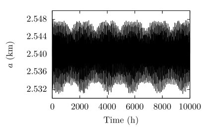
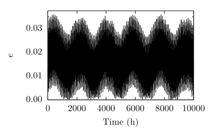
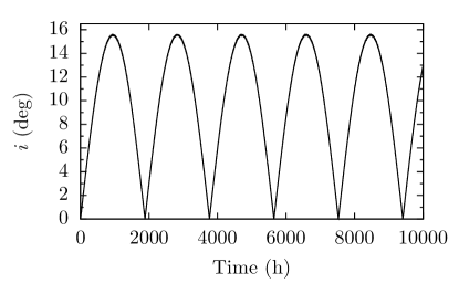
Figure 1 represents the orbital evolution of the system with respect to the initial orbital plane over $10\,000$h. The mutual potential is truncated at order 6. As observed by HSX16, the energy stored in the rotational motion is able to strongly influence the orbit by forcing its eccentricity and inclination to oscillate in the intervals $0\leq e\leq 0.035$ and $0\leq i\leq 16^{\circ}$, respectively. The total energy of the system is $8.7678\times 10^{10}$ J. Numerically, its variation is mainly due to the dissipative effect of the RKF integrator. Over the $10\,000$ h of integration time span, the total variation of the mechanical energy is only $-0.3870$ J, which is perfectly consistent with the $-0.3851$ J obtained by HSX16.

Refer to caption
Refer to caption
Refer to caption
Figure 1: Orbital evolution of the 1999 KW4 binary asteroid system over $10\,000$ h time span obtained with an RKF7(8) integrator with a fixed time step of 200 s. The mutual potential is truncated at order 6. $a$ is the semi-major axis, $e$ the eccentricity, and $i$ the inclination relative to the initial orbital plane.
Table 1: Computation time for a 200 h integration of the orbit using HSX16’s algorithm (first row) and our approach (second row).
Order 2 3 4 5 6 7 8 9
$t^{a}$ (sec) 0.2 0.7 2.1 6.6 17.3 42.6 99.3 206.0
$t^{b}$ (sec) 0.2 0.3 0.4 0.6 1.0 1.7 2.5 3.1

$t^{a}$ computation time using Hou et al’s algorithm on a single 2.9 GHz CPU frequency processor.
$t^{b}$ computation time using the present algorithm on a single 2.3 GHz CPU frequency processor.

A comparison of the integration times between our approach and the algorithm of HSX16 is presented in Table 1. The system is integrated over 20 000 h with a fixed time step of 200 s, and then the computation time is divided by 100 for a direct comparison with HSX16 who did the integration of the orbit over 200 h. Absolute CPU times highly depend on the compiler and the optimisation options. They should thus be compared with care. Nevertheless, both methods spend the same amount of computation time when the potential is truncated at the lowest order $n=2$. We can thus assume that the other columns of Tab. 1 objectively reflect the efficiency of the algorithms. Moreover, as the expansion order increases, the computation time growth differs significantly between the two methods. Ours proves to be much faster. At the 6th order of truncation, we already gain a factor 17 in speed, and at order 9, our approach only needs 3 seconds instead of the 3.4 minutes required by the algorithm of HSX16.

4 Conclusion

The decomposition of the mutual potential of two rigid bodies with arbitrary shape into spherical harmonics has sometimes been discarded because of the misconception that this formalism would involve trigonometric functions. However spherical harmonics do have expressions in terms of Cartesian coordinates. Moreover, not only recurrence relations allow to evaluate them efficiently, but the force and the orbital torque are easily computed by application of the gradient and the angular momentum operators, respectively. By consequence, if we restrain ourselves to the orbital part of the equations of motion only, our approach must be as efficient as a polynomial decomposition of the potential in Cartesian coordinates.

Nevertheless, numerical tests show that our algorithm is faster. The reason resides in the way rotations are handled. Here, we use the irreducible representation of the group SO(3) acting on the set of functions defined on the sphere, viz. Wigner D-matrices. These matrices have two advantages: they can be efficiently evaluated with recurrence relations and the torque is simply obtained by application of the spin operator. Combining spherical harmonics and Wigner D-matrices, we obtain an algorithm for which forces and torques are calculated as rapidly as the mutual potential.

In this work, in order to avoid singularities, rotations are parametrised using Cayley-Klein’s formalism whose parameters are strictly equivalent to quaternions. We make this choice because it is well adapted to the computation of Wigner D-matrices. Because this representation in not common in the celestial mechanics field, we briefly summarise the relation between these parameters and the standard 3-1-3 Euler angles. More properties can be found in textbooks on quantum theory of angular momentum (e.g., Varshalovich et al, 1988).

As a concluding remark, not only the present formalism allows to design a fast integrator for the full two rigid body problem, but it also reveals the underlying structure which is controlled by the group of rotations. This structure is often hidden in other approaches. We expect that this will allow to draw a more comprehensive view of the analytical problem.

References

  • Borderies (1978) Borderies N (1978) Mutual gravitational potential of N solid bodies. Celestial Mechanics 18:295–307, DOI 10.1007/BF01230170
  • Boué et al (2016) Boué G, Correia ACM, Laskar J (2016) Complete spin and orbital evolution of close-in bodies using a Maxwell viscoelastic rheology. Celestial Mechanics and Dynamical Astronomy DOI 10.1007/s10569-016-9708-x
  • Compère and Lemaître (2014) Compère A, Lemaître A (2014) The two-body interaction potential in the STF tensor formalism: an application to binary asteroids. Celestial Mechanics and Dynamical Astronomy 119:313–330, DOI 10.1007/s10569-014-9568-1
  • Fahnestock and Scheeres (2006) Fahnestock EG, Scheeres DJ (2006) Simulation of the full two rigid body problem using polyhedral mutual potential and potential derivatives approach. Celestial Mechanics and Dynamical Astronomy 96:317–339, DOI 10.1007/s10569-006-9045-6
  • Gimbutas and Greengard (2009) Gimbutas Z, Greengard L (2009) A fast and stable method for rotating spherical harmonic expansions. Journal of Computational Physics 228:5621 – 5627
  • Hartmann et al (1994) Hartmann T, Soffel MH, Kioustelidis T (1994) On the use of STF-tensors in celestial mechanics. Celestial Mechanics and Dynamical Astronomy 60:139–159, DOI 10.1007/BF00693097
  • Hou et al (2016) Hou X, Scheeres DJ, Xin X (2016) Mutual Potential between Two Rigid Bodies with Arbitrary Shapes and Mass Distributions. Celestial Mechanics and Dynamical Astronomy pp 1–27, DOI 10.1007/s10569-016-9731-y
  • Maciejewski (1995) Maciejewski AJ (1995) Reduction, Relative Equilibria and Potential in the Two Rigid Bodies Problem. Celestial Mechanics and Dynamical Astronomy 63:1–28, DOI 10.1007/BF00691912
  • Mathis and Le Poncin-Lafitte (2009) Mathis S, Le Poncin-Lafitte C (2009) Tidal dynamics of extended bodies in planetary systems and multiple stars. Astron. Astrophys. 497:889–910, DOI 10.1051/0004-6361/20079054
  • Paul (1988) Paul MK (1988) An Expansion in Power Series of Mutual Potential for Gravitating Bodies with Finite Sizes. Celestial Mechanics 44:49–59, DOI 10.1007/BF01230706
  • Poincaré (1901) Poincaré H (1901) Sur une forme nouvelle des équations de la mécanique. Comptes rendus de l’Académie des Sciences 132:369–371
  • Tricarico (2008) Tricarico P (2008) Figure figure interaction between bodies having arbitrary shapes and mass distributions: a power series expansion approach. Celestial Mechanics and Dynamical Astronomy 100:319–330, DOI 10.1007/s10569-008-9128-7, 0711.2078
  • Varshalovich et al (1988) Varshalovich D, Moskalev A, Khersonskii V (1988) Quantum Theory of Angular Momentum. World Scientific
  • Werner and Scheeres (2005) Werner RA, Scheeres DJ (2005) Mutual Potential of Homogeneous Polyhedra. Celestial Mechanics and Dynamical Astronomy 91:337–349, DOI 10.1007/s10569-004-4621-0
  • Wigner (1959) Wigner EP (1959) Group theory and its application to the quantum mechanics of atomic spectra. Academic Press, New York