Entanglement and coherence in a spin-$s$ $XXZ$ system under non-uniform fields

Abstract

We investigate entanglement and coherence in an $XXZ$ spin-$s$ pair immersed in a non-uniform transverse magnetic field. The ground state and thermal entanglement phase diagrams are analyzed in detail in both the ferromagnetic and antiferromagnetic cases. It is shown that a non-uniform field enables to control the energy levels and the entanglement of the corresponding eigenstates, making it possible to entangle the system for any value of the exchange couplings, both at zero and finite temperatures. Moreover, the limit temperature for entanglement is shown to depend only on the difference $|h_{1}-h_{2}|$ between the fields applied at each spin, leading for $T>0$ to a separability stripe in the $(h_{1},h_{2})$ field plane such that the system becomes entangled above a threshold value of $|h_{1}-h_{2}|$. These results are demonstrated to be rigorously valid for any spin $s$. On the other hand, the relative entropy of coherence in the standard basis, which coincides with the ground state entanglement entropy at $T=0$ for any $s$, becomes non-zero for any value of the fields at $T>0$, decreasing uniformly for sufficiently high $T$. A special critical point arising at $T=0$ for non-uniform fields in the ferromagnetic case is also discussed.
Keywords: Quantum Entanglement, Quantum Coherence, Spin Systems, Non-uniform fields

1 Introduction

The theory of quantum entanglement has provided a useful and novel perspective for the analysis of correlations and quantum phase transitions in interacting many body systems [1, 2, 3, 4, 5]. At the same time, it is essential for determining the capability of such systems for performing different quantum information tasks [6, 7, 8]. More recently, a general theory of quantum resources, similar to that of entanglement but based on the degree of coherence of a quantum system with respect to a given reference basis, was proposed [9, 10, 11, 12]. Thus, entanglement and coherence provide a means to capture the degree of quantumness of a given quantum system.

In particular, spin systems constitute paradigmatic examples of strongly interacting many body systems which enable to study in detail the previous issues, providing at the same time a convenient scalable scenario for the implementation of quantum information protocols. Interest on spin systems has been recently enhanced by the significant advances in control techniques of quantum systems, which have permitted the simulation of interacting spin models with different type of couplings by means of trapped ions, Josephson junctions or cold atoms in optical lattices [13, 14, 15, 16, 17, 18].

Accordingly, interacting spin systems have been the object of several relevant studies. Entanglement and discord-type correlations [19, 20, 21, 22] in spin pairs and chains with Heisenberg couplings under uniform fields were intensively investigated, specially for spin $1/2$ systems [3, 23, 24, 25, 26, 27, 28, 29, 30, 31, 32, 33, 34]. The effects of non-uniform fields have also received attention, mostly for spin $1/2$ systems [35, 36, 37, 38, 39, 40, 41, 42], although some results for higher spins in non-uniform fields are also available [43, 44, 45].

The aim of this work is to analyze in detail the effects of a non-uniform magnetic field on the entanglement and coherence of a spin-$s$ pair interacting through an $XXZ$ coupling, both at zero and finite temperature. We examine the interplay between the non-uniform magnetic field and temperature and their role to control quantum correlations. We also study the critical behaviour and the development of different phases as the spin increases, when the field, temperature, and coupling anisotropy are varied. Analytical rigorous results are also provided. In particular, the $T=0$ phase diagram will be characterized by ground states of definite magnetization $M$, all reachable through non-uniform fields for any value of the couplings, with entanglement decreasing with increasing $|M|$. Special critical points will be discussed. On the other hand, the limit temperature for entanglement will be shown to depend, for any value of $s$, only on the difference between the fields applied at each spin, leading to a thermal phase diagram characterized by a separability stripe in field space. Finally, we will analyze the relative entropy of coherence [10] in the standard basis, which coincides here exactly with the entanglement entropy at $T=0$ but departs from entanglement as $T$ increases.

The model and results are presented in sections II–IV, starting with the basic spin $1/2$ case and considering then the $s=1$ and the general spin-$s$ cases. Conclusions are finally given in section V.

2 Model and the spin 1/2 case

We consider a spin $s$ pair interacting through an $XXZ$-type coupling, immersed in a transverse magnetic field $\bm{h}$ not necessarily uniform. The Hamiltonian can be written as

$$H=-h_{1}s_{1}^{z}-h_{2}s_{2}^{z}+J(s_{1}^{x}s_{2}^{x}+s_{1}^{y}s_{2}^{y})+J_{z}s_{1}^{z}s_{2}^{z}\,,$$ (1)

where $s^{\mu}_{i}$ ($\mu=x,y,z$) denote the (dimensionless) spin operators at site $i$ and $J$, $J_{z}$ the exchange couplings, with $J_{z}/J$ the anisotropy ratio. This Hamiltonian commutes with the total spin along the $z$ axis, $S_{z}=s^{z}_{1}+s^{z}_{2}$, having then eigenstates with definite magnetization $M$ along $z$. Without loss of generality, we will set in what follows $J>0$, as its sign can be changed by a local rotation of angle $\pi$ around the $z$ axis of one of the spins, which will not affect the energy spectrum nor the entanglement of its eigenstates. The ferromagnetic (FM) case $J<0$, $J_{z}<0$ is then equivalent to $J>0$, $J_{z}<0$.

We also remark that a Hamiltonian with an additional Dzyaloshinskii-Moriya coupling along $z$ [46], $H^{\prime}=H+D\sum_{i}(s_{i}^{x}s_{i+1}^{y}-s_{i}^{y}s_{i+1}^{x})$, can be transformed back exactly into a Hamiltonian (1) with $J\rightarrow J^{\prime}=\sqrt{J^{2}+D^{2}}$, by means of a rotation of angle $\phi=\tan^{-1}(D/J)$ around the $z$ axis at the second spin [47]. Hence, its spectrum and entanglement properties will also coincide exactly with those of Eq. (1) for $J\rightarrow J^{\prime}$.

We first review the $s=1/2$ case, providing a complete study with analytical results and including coherence in the standard basis, which allows to understand more easily the general spin $s$ case, considered in the next subsections. Entanglement and discord-type correlations under non homogeneous fields in a spin $1/2$ pair were studied in [35, 39] for an $XX$-type coupling, in [36] for an isotropic coupling, in [37, 40] for an $XXZ$ coupling and in [41] for an $XYZ$ coupling.

2.1 The spin $1/2$ pair

Using qubit notation, the eigenstates of the Hamiltonian (1) for $s=1/2$ are the separable aligned states $|00\rangle\equiv|\uparrow\uparrow\rangle$ and $|11\rangle\equiv|\downarrow\downarrow\rangle$, with magnetization $M=\pm 1$ and energies

$$E_{\pm 1}=\mp\frac{1}{2}(h_{1}+h_{2})+\frac{1}{4}J_{z}\,,$$ (2)

and the entangled $M=0$ states $\left|\Psi^{\pm}\right\rangle=\cos\alpha_{\pm}|01\rangle+\sin\alpha_{\pm}|10\rangle$, with energies

$$E_{0}^{\pm}=\pm\frac{1}{2}\Delta-\frac{1}{4}J_{z}\,,\;\;\Delta=\sqrt{(h_{1}-h_{2})^{2}+J^{2}}\,,$$ (3)

and $\tan\alpha_{\pm}=\frac{h_{1}-h_{2}\pm\Delta}{J}$. The concurrence [48] of these states is given by

$$C\left(\left|\Psi^{\pm}\right\rangle\right)=|\sin 2\alpha_{\pm}|=J/\Delta\,,$$ (4)

and is a decreasing function of $|h_{1}-h_{2}|/J$. Their entanglement entropy, $S=-{\rm Tr}\rho_{i}\log_{2}\rho_{i}$ with $\rho_{i}$ the reduced state of one of the spins, can then be obtained as

$${\textstyle S=-\sum_{\nu=\pm}p_{\nu}\log_{2}p_{\nu}\,,\;\;p_{\pm}=\frac{1\pm\sqrt{1-C^{2}}}{2}}\,,$$ (5)

and is an increasing function of $C$. In the uniform case $h_{1}=h_{2}$, $\left|\Psi^{\pm}\right\rangle$ become the Bell states $\frac{\left|01\right\rangle\pm\left|10\right\rangle}{\sqrt{2}}$ and $S(|\Psi^{\pm})=C(|\Psi^{\pm}\rangle)=1$.

Through a non-uniform field it is then possible to tune the entanglement of the $M=0$ eigenstates, decreasing it by applying a field difference. On the other hand, such difference also decreases the energy $E_{0}^{-}$ of $|\Psi^{-}\rangle$ and increases that of $|\Psi^{+}\rangle$, without affecting that of the aligned eigenstates if the average field is kept constant, enabling to have the entangled state $|\Psi^{-}\rangle$ as a non-degenerate ground state (GS) for any value of $J$ or $J_{z}$. A similar effect can be obtained by increasing $J_{z}$, which increases the gap between the entangled and the aligned states, in this case without affecting their concurrence.

Eqs. (2)–(3) then lead to the phase diagrams of Fig. 1. For clarity we have considered the whole field plane, although the diagrams are obviously symmetric under reflection from the $h_{1}=h_{2}$ line (and spectrum and entanglement also from the $h_{1}=-h_{2}$ line). The GS will be either the entangled state $|\Psi^{-}\rangle$ (red sector) or one of the aligned states ($|00\rangle$ if $h_{1}+h_{2}>0$ or $|11\rangle$ if $h_{1}+h_{2}<0$, white sectors), with $|\Psi^{-}\rangle$ a non-degenerate GS ($E_{0}^{-}<E_{\pm 1}$) if and only if

$$|h_{1}+h_{2}|<J_{z}+\sqrt{J^{2}+(h_{1}-h_{2})^{2}}.$$ (6)

This equation is equivalent to the following conditions:

$$\!\!\!\!(h_{1}-{\textstyle\frac{J_{z}}{2}})(h_{2}-{\textstyle\frac{J_{z}}{2}}) < {\textstyle\frac{J^{2}}{4}}\,,\;\;(h_{1}+h_{2}\geq 0,\;h_{1}>{\textstyle\frac{J_{z}}{2}})$$ (7)

$$\!\!\!\!(h_{1}+{\textstyle\frac{J_{z}}{2}})(h_{2}+{\textstyle\frac{J_{z}}{2}}) < {\textstyle\frac{J^{2}}{4}}\,,\;\;(h_{1}+h_{2}\leq 0,\;h_{1}<\!-{\textstyle\frac{J_{z}}{2}})\,.$$ (8)

which show that the borders of the entangled sector are displaced hyperbola branches.

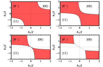
Figure 1: Ground state phase diagram for the spin $1/2$ pair. Top: antiferromagnetic (AFM) case $J_{z}=J$ (left) and ferromagnetic (FM)-type case $J_{z}=-J/2$ (right). Bottom: FM cases $J_{z}=-J$ (left) and $J_{z}=-\frac{3}{2}J$ (right).

In the AFM case $J_{z}>0$, the diagram has the form of the top left panel. Here the GS is entangled at zero field and if one of the fields is sufficiently weak ($|h_{1}|<J_{z}/2$) the GS remains entangled for any value of the other field. However, in the FM case $J_{z}<0$ two distinct diagrams can arise (top and bottom right panels), separated by the limit diagram of the bottom left panel ($J_{z}=-J$). If $-J<J_{z}<0$ (top right), the system is still entangled at zero field but now if one of the fields is sufficiently weak ($|h_{1}|<|J_{z}|/2$, dashed vertical lines) entanglement is confined to a finite interval of the other field. Control of just one field then allows to switch entanglement on and off for any value of the other field.

On the other hand, if $J_{z}<-J$, the GS is aligned for any uniform non-zero field, and $|\Psi^{-}\rangle$ becomes GS only above a threshold value of the field difference, $|h_{1}-h_{2}|>\sqrt{J_{z}^{2}-J^{2}}$ (Eq. (6)), within the limits determined by Eqs. (6)–(8). These limits imply that the sign of the field at each site must be different, as seen in the bottom right panel. Hence, GS entanglement is in this case switched on (rather than destroyed) by field application, provided it has opposite signs at each spin. In addition, a GS transition between the aligned states $|11\rangle$ and $|00\rangle$ takes place at the line $h_{1}=-h_{2}$ for $|h_{1}-h_{2}|<\sqrt{J_{z}^{2}-J^{2}}$, with the GS degenerate in this interval along this line.

The GS concurrence for the same cases of Fig. 1 is depicted on Fig. 2. As seen in the top panels, the maximum $C=1$ is reached for $h_{1}=h_{2}=h$ provided $J_{z}>-J$ and $|h|<\frac{J+J_{z}}{2}$. For $J_{z}<-J$, the maximum value is $C=J/|J_{z}|<1$, attained at the edges $h_{1}=-h_{2}=\pm\frac{1}{2}\sqrt{J_{z}^{2}-J^{2}}$ of the entangled sector.

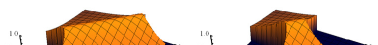
Figure 2: Concurrence of the GS as a function of the magnetic fields for the cases of Fig. 1. Top: $J_{z}=J$ (left) and $-J/2$ (right). Bottom: $J_{z}=-J$ (left) and $-\frac{3}{2}J$ (right).

2.1.1 Thermal entanglement

Let us now consider a finite temperature $T$. As $T$ increases from 0, an entangled GS will become mixed with other excited states, leading to a decrease of the entanglement which will vanish beyond a limit temperature. However, if the GS is separable, the thermal state can become entangled for $T>0$ (below some limit temperature) due to the presence of entangled excited states, implying that the entanglement phase diagram for $T>0$ may differ from that at $T=0$ even for low $T$.

In the present case the thermal state $\rho_{12}=Z^{-1}e^{-\beta H}$, with $Z={\rm Tr}\,e^{-\beta H}$ the partition function and $\beta=1/kT$, has in the standard basis the form

$$\rho_{12}=\left(\begin{array}[]{cccc}p_{+}&0&0&0\\ 0&q_{+}&w&0\\ 0&w&q_{-}&0\\ 0&0&0&p_{-}\end{array}\right)\,,$$ (9)

where $p_{\pm}=Z^{-1}e^{-\beta E_{\pm 1}}$, $q_{\pm}=Z^{-1}e^{\beta J_{z}/4}(\cosh\frac{\beta\Delta}{2}\pm\frac{h_{1}-h_{2}}{\Delta}\sinh\frac{\beta\Delta}{2})$ and $w=-Z^{-1}e^{\beta J_{z}/4}\frac{J}{\Delta}\sinh\frac{\beta\Delta}{2}$. Its concurrence [48] is then given by

$$C = 2{\rm Max}[|w|-\sqrt{p_{+}p_{-}},0]={\textstyle 2Z^{-1}{\rm Max}[\frac{J}{\Delta}e^{\beta J_{z}/4}\sinh\frac{\beta\Delta}{2}-e^{-\beta J_{z}/4},0]}\,.$$ (10)

Thus, for $T>0$ $\rho_{12}$ is entangled if and only if

$${\frac{J}{\Delta}e^{\beta J_{z}/2}\sinh\frac{\beta\Delta}{2}>1}\,.$$ (11)

Eq. (11) implies a limit temperature for entanglement that will depend on $J_{z}$, $J$ and $|h_{1}-h_{2}|$ only. It also implies a threshold value of $J_{z}$ for entanglement at any $T>0$,

$$J_{z}>2kT\ln\frac{\Delta/J}{\sinh\frac{\beta\Delta}{2}}=-\Delta+4kT\ln\frac{\Delta/J}{1-e^{-\beta\Delta}}\,.$$ (12)

Hence, it is always possible to entangle the thermal state by increasing $J_{z}$, since it will effectively cool down the system to the state $|\Psi^{-}\rangle$, as previously stated.

The same effect occurs if the field difference $|h_{1}-h_{2}|$ is increased. The left hand side of Eq. (11) is an increasing function of $\Delta$ and hence of $|h_{1}-h_{2}|$ for any $T>0$ and $J_{z}$, so that at any $T>0$ there will also exist a threshold value $h_{c}$ of the field difference $|h_{1}-h_{2}|$ above which the thermal state will become entangled:

$$|h_{1}-h_{2}|>h_{c}(T,J,J_{z})\,.$$ (13)

Eq. (13) gives rise to a separability stripe $|h_{1}-h_{2}|\leq h_{c}(T,J,J_{z})$, as depicted in Fig. 3. Here $h_{c}(T,J,J_{z})=\sqrt{\Delta_{c}^{2}-J^{2}}$, with $\Delta_{c}=2kTf^{-1}(\frac{2kT}{J}e^{-\beta J_{z}/2})$ and $f^{-1}$ the inverse of the increasing function $f(x)=\sinh x/x$ ($x>0$).

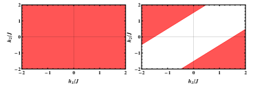
Figure 3: Thermal entanglement phase diagram for the spin $1/2$ pair at $kT=J/2$. Left: AFM case $J_{z}=J$. Right: FM case $J_{z}=-J/2$. Red sectors indicate entanglement. The whole plane remains entangled for $0<kT<0.91J$ if $J_{z}=J$ and $0<kT<0.335J$ if $J_{z}=-J/2$. Above these temperatures, a separability stripe $|h_{1}-h_{2}|\leq h_{c}(T,J,J_{z})$ arises. For $J_{z}<-J$ the separability stripe arises for any $T>0$.

Eq. (13) implies that the thermal entanglement phase diagram in the field plane differs from the $T=0$ phase diagram even for small temperatures $T>0$, as it is determined just by the field difference $|h_{1}-h_{2}|$. Entanglement will be turned on in $T=0$ separable sectors outside the stripe as soon as $T$ becomes finite. In particular, for $J_{z}>-J$, Eq. (12) shows that in contrast with the $T=0$ case, the whole $h_{1},h_{2}$ plane becomes entangled for $0<T<T_{c}$, with $T_{c}(J,J_{z})$ determined by

$$e^{\beta_{c}J_{z}/2}\sinh{\textstyle\frac{\beta_{c}J}{2}}=1\,,$$ (14)

such that $h_{c}(T,J,J_{z})=0$ if $T<T_{c}(J,J_{z})$. The separability stripe arises then for $T>T_{c}(J,J_{z})$. For $J_{z}\rightarrow-J$, $T_{c}\rightarrow 0$ while if $J_{z}=0$, $kT_{c}=\frac{1}{2}J/{\rm arcsinh}\,1\approx 0.567J$.

However, for $J_{z}<-J$ a separability stripe will be present for all $T>0$, with $h_{c}(T,J,J_{z})\rightarrow\sqrt{J_{z}^{2}-J^{2}}$ for $T\rightarrow 0^{+}$. The thermal phase diagram in the field plane is then characterized, for any value of $J_{z}$, by a separability stripe whose width increases with increasing $T$, and vanishes for $J_{z}>-J$ if $T<T_{c}(J,J_{z})$.

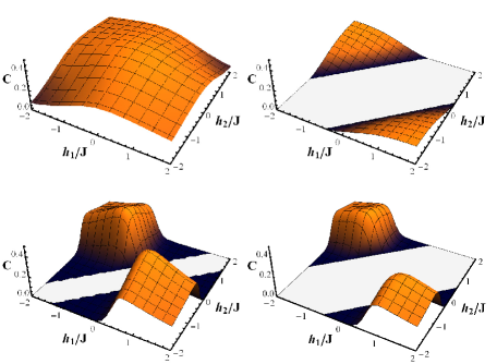
Figure 4: Concurrence as a function of the magnetic fields $h_{1}$ and $h_{2}$ at finite temperature. Top panels: AFM case $J_{z}=J$ (left) and FM case $J_{z}=-J/2$ (right) at temperature $kT=J/2$. Bottom panels: Same diagrams for the FM cases $J_{z}=-J$ (left) and $J_{z}=-\frac{3}{2}J$ (right) at $kT=0.05J$.

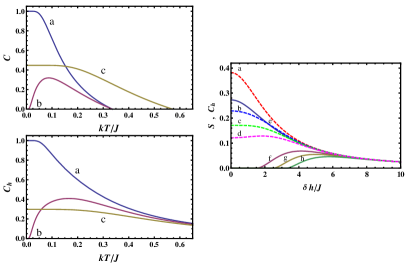
Figure 5: Left: Concurrence (upper panel) and relative entropy of coherence in the standard basis (lower panel) as a function of temperature for $J_{z}=-J/2$ at $h_{1}=h_{2}=0$ (a), $h_{1}=h_{2}=0.3J$ (b) and $h_{1}=-h_{2}=J$ (c). The reentry of entanglement for $T>0$ in case (b) is clearly seen, with the limit temperature for entanglement independent of the field if $h_{1}=h_{2}$ (cases a,b) and increasing with increasing values of $|h_{1}-h_{2}|$ (case c), as follows from Eq. (11). In contrast, the coherence remains non-zero $\forall$ $T$, decreasing uniformly as $(J/kT)^{2}$ for high $T$ (Eq. 16) and approaching the entanglement entropy (5) for $T\rightarrow 0$. Right: Entanglement of formation $S$ (solid lines) and relative entropy of coherence (dashed lines) as a function of the field difference $\delta h=|h_{1}-h_{2}|$ at fixed temperature $kT=J/2$ for $J_{z}/J=1$ (a,e), $-1/2$ (b,f), $-1$ (c,g) and $-3/2$ (d,h), at $h_{1}=-h_{2}$. As $|\delta h|$ increases, all curves coalesce and become independent of $J_{z}$, approaching the entanglement entropy of the GS $|\Psi^{-}\rangle$ determined by Eq. (4).

The thermal concurrence is shown in Fig. 4. It is verified that it is strictly zero just within the separability stripe (13), becoming small but non-zero in the $T=0$ separable regions outside it (dark blue in Fig. 4). Nonetheless, such reentry of entanglement for $T>0$ can become quite noticeable in some cases, as seen in the top panel of Fig. 5. It is also verified that through non-uniform fields it becomes possible to preserve entanglement up to temperatures higher than those in the uniform case (which lies at the center of the separability stripe), as also seen in Fig. 5.

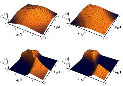
Figure 6: Relative entropy of coherence in the standard basis as a function of the transverse non-uniform fields $h_{1}$ and $h_{2}$ at finite temperatures, for the same cases of Fig. 4. Top panels: AFM case $J_{z}=J$ (left) and FM case $J_{z}=-J/2$ (right) for $kT=J/2$. Bottom panels: FM cases $J_{z}=-J$ (left) and $J_{z}=-\frac{3}{2}J$ (right) for $kT=0.1J$.

2.1.2 Coherence

We now analyze the coherence of the thermal state (9) with respect to the standard product basis $\{|00\rangle,|01\rangle,|10\rangle,|11\rangle\}$. This quantity can be measured through the relative entropy of coherence [10], defined as

$$C_{h}(\rho_{12})=S(\rho_{12}||\rho_{12}^{\rm diag})=S(\rho_{12}^{\rm diag})-S(\rho_{12}),$$ (15)

where $S(\rho)=-{\rm Tr}\rho\log_{2}\rho$ is the von Neumann entropy and $\rho_{12}^{\rm diag}$ its diagonal part in the previous basis. It is a measure of the strength of the off-diagonal elements in this basis, and would obviously vanish if $J=0$. It will be here driven just by the coefficient $w$ in (9). A series expansion of (15) for $|w|\ll q_{\pm}$ in (9) leads in fact to $C_{h}(\rho_{12})\approx\frac{\log_{2}(q_{+}/q_{-})}{q_{+}-q_{-}}\,w^{2}$. The exact expression is $C_{h}(\rho_{12})=-\sum_{\nu=\pm}(q_{\nu}\log_{2}q_{\nu}-p^{0}_{\nu}\log_{2}p^{0}_{\nu})$, where $p^{0}_{\pm}=Z^{-1}e^{-\beta E_{0}^{\pm}}$.

In the zero temperature limit, $S(\rho_{12})$ vanishes while $S(\rho_{12}^{\rm diag})$ and hence $C_{h}(\rho_{12})$ become the entanglement entropy $S$ of the GS, Eq. (5), since the standard basis is here the Schmidt basis for $|\Psi^{-}\rangle$. However, for $T>0$, $C_{h}(\rho_{12})$ becomes everywhere non-zero due to the non-vanishing weight of the entangled states $|\Psi^{\pm}\rangle$, as seen in Figs. 5 and 6. In fact, for $kT\gg{\rm max}[J,J_{z},h_{1},h_{2}]$, a series expansion leads to the asymptotic expression

$$C_{h}(\rho_{12}) \approx {\textstyle\frac{1}{16\ln 2}\left(\frac{J}{kT}\right)^{2}\left[1+\frac{J_{z}}{4kT}-\frac{3[(h_{1}+h_{2})^{2}+J^{2}]+(h_{1}-h_{2})^{2}}{48(kT)^{2}}\right]}\,,$$ (16)

showing that it ultimately decreases uniformly as $(J/kT)^{2}$ in this limit. It then exhibits a reentry for $T>0$ in all $T=0$ separable sectors, as seen in Figs. 5 and 6.

As previously mentioned, by applying sufficiently strong opposite fields at each site it is possible to effectively “cool down” the thermal state $\rho_{12}$ at any $T>0$, bringing it as close as desired to the entangled state $|\Psi^{-}\rangle\langle\Psi^{-}|$. This behaviour is shown in the right panel of Fig. 5. It is seen that the entanglement of formation $S$, obtained from the thermal concurrence $C$ by the same expression (5) [48], and the relative entropy of coherence, initially different and dependent on $J_{z}$, merge for increasing values of $|h_{1}-h_{2}|$, approaching a common $J_{z}$-independent limit which is the entanglement entropy $S$ of the pure state $|\Psi^{-}\rangle$. The vanishing difference between $S$ and $C_{h}$ for high $|h_{1}-h_{2}|$ is a clear signature that $\rho_{12}$ has become essentially pure.

3 The spin-$1$ pair

We now consider the $s=1$ case. The behaviour is essentially similar to that for $s=1/2$, the main difference being the appearing of an intermediate $M=\pm 1$ magnetization step in the $T=0$ diagrams, between the entangled $M=0$ GS and the aligned separable $M=\pm 2$ states. This effect leads to an entanglement step since the $M=\pm 1$ GS is less entangled than the $M=0$ GS.

Using now the notation $|m_{1},m_{2}\rangle$ for the states of the standard basis, with $m_{i}$ the eigenvalues of $s_{i}^{z}$, the GS of the spin $1$ $XXZ$ pair can be one of the $|M|=2$ aligned states $|\Psi_{\pm 2}\rangle=|\pm 1,\pm 1\rangle$, one of the $|M|=1$ states, which will be of the form

$$|\Psi_{\pm 1}\rangle=\cos\alpha_{\pm}|\pm 1,0\rangle+\sin\alpha_{\pm}|0,\pm 1\rangle\,,$$ (17)

with $\tan\alpha_{\pm}=\pm\frac{\eta}{2}-\sqrt{1+\frac{\eta^{2}}{4}}$ and $\eta=\frac{h_{1}-h_{2}}{J}$, and one of the $M=0$ states, of the form

$$|\Psi_{0}\rangle=\gamma_{+}|1,-1\rangle+\gamma_{0}|00\rangle+\gamma_{-}|-1,1\rangle\,.$$ (18)

‘ All coefficients are independent of $h_{1}+h_{2}$, but those of $|\Psi_{0}\rangle$ depend now on $J_{z}$. For $J_{z}=0$ they can be still written down concisely: $\gamma_{0}/\gamma_{+}=\eta-\sqrt{2+\eta^{2}}$, $\gamma_{-}/\gamma_{+}=1+\eta\gamma_{0}/\gamma_{+}$.

Their energies are

$$E_{\pm 2} = \mp(h_{1}+h_{2})+J_{z}\,,$$

$$E_{\pm 1} = {\textstyle\mp\frac{h_{1}+h_{2}}{2}-\sqrt{J^{2}+(\frac{h_{1}-h_{2}}{2})^{2}}}\,,$$ (19)

$$E_{0} = -\sqrt{2J^{2}+(h_{1}-h_{2})^{2}}\;\;\;\;\;\;\;(J_{z}=0)\,.$$ (20)

The border of the $T=0$ entangled region, determined by that between the $|M|=2$ and $|M|=1$ GS, $E_{\pm 2}=E_{\pm 1}$, is then given again by Eqs. (6)–(8) with $J\rightarrow 2J$, $J_{z}\rightarrow 2J_{z}$. The GS phase diagrams have then the same forms as those of Fig. 1 except for the previous rescaling and the magnetization step. The $J_{z}=0$ case is shown in Fig. 7.

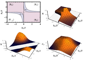
Figure 7: Top: Ground state phase diagram (left) and negativity (right) for the spin $1$ pair with $J_{z}=0$ as a function of the applied fields at each spin. Colored sectors on the left indicate entanglement. Bottom: The negativity (left) and relative entropy of coherence (right) of the thermal state of the spin $1$ pair at temperature $kT=J$ as a function of the applied fields.

As entanglement measure valid for both zero and finite temperature, we will now use the negativity [49, 50], a well-known entanglement monotone which is computable in any mixed state, since an explicit expression for the concurrence or entanglement of formation of a general mixed state of two qutrits (spin $1$ pair) or in general two qudits with $d\geq 3$ is no longer available. The negativity is minus the sum of the negative eigenvalues of the partial transpose [51, 52] $\rho_{12}^{\rm t_{2}}$ of $\rho_{12}$:

$$N(\rho_{12})=({\rm Tr}|\rho_{12}^{\rm t_{2}}|-1)/2\,.$$ (21)

A non-zero negativity implies entanglement, whereas for mixed states, the converse is not necessarily true (except for two qubit states [51, 52] or special states), vanishing for bound entangled states. Nonetheless it is normally used as an indicator of useful entanglement.

For pure states it reduces to a special entanglement entropy [31], being a function of the one-spin reduced state $\rho_{1}$ (or $\rho_{2}$, isospectral with $\rho_{1}$ for a pure state): $N=\frac{1}{2}[({\rm Tr}\,\sqrt{\rho_{1}})^{2}-1]$. It is then non-zero if and only if the state is entangled. Its maximum value for a spin $s$ pair is $N=s$. We then obtain $N(|\Psi_{\pm 2}\rangle)=0$,

$$N(|\Psi_{\pm 1}\rangle) = {\textstyle\frac{1}{2}|\sin(2\alpha_{\pm})|=\frac{1}{\sqrt{4+\eta^{2}}}}\,,$$ (22)

$$N(|\Psi_{0}\rangle) = {\textstyle\frac{1}{2}}[|\gamma_{+}\gamma_{-}|+|\gamma_{0}|(|\gamma_{+}|+|\gamma_{-}|)]$$ (23)

$$= {\textstyle\frac{1+\sqrt{2}\sum\limits_{\nu=\pm}\sqrt{1+\eta(\eta+\nu\sqrt{2+\eta^{2}})}}{2(2+\eta^{2})}}\;\;\;\;\;(J_{z}=0)\,.$$ (24)

They are decreasing functions of $\eta=\frac{h_{1}-h_{2}}{J}$, reaching for $\eta=0$ the value $\frac{1}{2}$ for $|M|=1$ (maximum value for Schmidt rank $2$) and $\frac{1+2\sqrt{2}}{4}\approx 0.958$ for $M=0$. The negativity of the $M=0$ GS depends now on $J_{z}$, reaching the maximum $N=1$ for $J_{z}=1$.

It is verified in Fig. 7 that the $T=0$ phase diagram and entanglement for $J_{z}=0$ is similar to that for $s=1/2$ except for the $M=\pm 1$ magnetization and negativity steps. Remarkably, the finite temperature negativity diagram is again characterized by a separability stripe $|h_{1}-h_{2}|\leq h_{c}(T,J,J_{z})$ for $T>T_{c}$, with the boundary of the non-zero negativity sector independent of $h_{1}+h_{2}$ (as demonstrated in the next section). At $J_{z}=0$ the stripe emerges for $kT>kT_{c}\approx 0.864J$ (root of the critical equation $3+2\cosh(2\beta_{c}J)=\cosh(2\sqrt{2}\beta_{c}J)$), with the whole field plane entangled for $T<T_{c}$. It should be also mentioned that the $T=0$ negativity step gives rise to a negativity “valley” for low finite $T$ due to the convexity of $N$, as will be seen in the next section.

The relative entropy of coherence in the standard basis behaves in the same way as before. It approaches the GS entanglement entropy for $T\rightarrow 0$, while for $kT\gg J,J_{z},|h_{1}|,|h_{2}|$, it decreases uniformly at leading order, becoming, for $J_{z}=0$,

$$C_{h}(\rho_{12})\approx{\textstyle\frac{4}{9\ln 2}(\frac{J}{kT})^{2}[1-\frac{55J^{2}+15(h_{1}+h_{2})^{2}+9(h_{1}-h_{2})^{2}}{(12kT)^{2}}]}\,.$$ (25)

4 The spin $s$ case

4.1 Ground state phase diagram and entanglement

Let us finally consider the main features of the general spin $s$ $XXZ$ pair in a non-uniform field. The GS phase diagram remains similar to the previous cases, but now with $2s$ magnetization steps, from $M=0$ up to $M=\pm 2s$. These steps originate $2s$ steps in the $T=0$ entanglement and negativity, since they decrease with increasing $|M|$. This behaviour can be seen in the top panels of Fig. 8 for an $s=2$ pair.

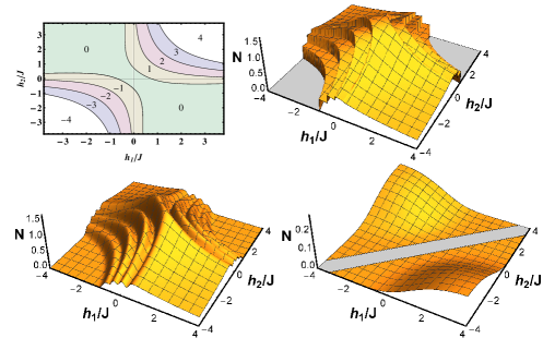
Figure 8: Top: Ground state phase diagram (left) and negativity (right) for a spin $2$ pair with $J_{z}=0$ as a function of the applied fields at each spin. Colored sectors on the left indicate entanglement, with the number denoting the magnetization of the state. Bottom: The negativity of the spin 2 pair at temperature $kT=0.1J$ (left) and $kT=1.6J$ (right).

The border of the entangled region in the field plane is determined by that between the aligned GS with $|M|=2s$ and the entangled GS with $|M|=2s-1$. Remarkably, it is the same as that for $s=1/2$, Eq. (6), with the rescaling $J\rightarrow 2sJ$, $J_{z}\rightarrow 2sJ_{z}$:

$$|h_{1}+h_{2}|<2sJ_{z}+\sqrt{4s^{2}J^{2}+(h_{1}-h_{2})^{2}}\,.$$ (26)

The border are then the hyperbolas (7)–(8) with the previous scaling and give rise to the same possibilities depicted in Fig. 1, with the additional inner magnetization steps.
Proof: Considering first $h_{1}+h_{2}\geq 0$, the energies of the $M=2s$ aligned state $|ss\rangle$ and the lowest $M=2s-1$ state, which is $|\Psi_{2s-1}\rangle=\cos\alpha|s,s-1\rangle+\sin\alpha|s-1,s\rangle$, with $\tan\alpha=\frac{\eta}{2s}-\sqrt{1+\frac{\eta^{2}}{4s^{2}}}$ and $\eta=\frac{h_{1}-h_{2}}{J}$, are

$$E_{2s} = -{\textstyle s(h_{1}+h_{2})+s^{2}J_{z}}\,,$$ (27)

$$E_{2s-1} = {\textstyle-(2s-1)\frac{h_{1}+h_{2}}{2}+s(s-1)J_{z}-\sqrt{(\frac{h_{1}-h_{2}}{2})^{2}+s^{2}J^{2}}}\,.$$ (28)

The condition $E_{2s-1}<E_{2s}$ leads then to Eq. (26). If $h_{1}+h_{2}\leq 0$, the result is similar with $h_{1}+h_{2}$ replaced by $|h_{1}+h_{2}|$ and $E_{M}$ by $E_{-M}$. ∎

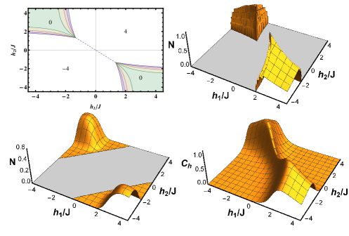
Figure 9: Top: Ground state phase diagram (left) and negativity (right) for a spin $2$ pair with $J_{z}=-1.2J$ as a function of the applied fields at each spin. Colored sectors indicate an entangled GS, with the color and number identifying the distinct magnetizations. Bottom: The negativity (left) and relative entropy of coherence (right) of the spin 2 pair for $J_{z}=-1.2J$ at temperature $kT=0.5J$.

In Fig. 9 we plot an example for $s=2$ of the interesting FM case $J_{z}<-J$, where the GS is fully aligned for any uniform field $h_{1}=h_{2}=h$, as in the $s=1/2$ case, with a transition $M=-2s$ to $M=2s$ at $h=0$. However, it can again be entangled with a non-uniform field, by applying opposite fields at each spin. Eq. (26) implies that in this case GS entanglement will arise for

$$|h_{1}-h_{2}|>h_{c}=2s\sqrt{J_{z}^{2}-J^{2}}\,\;\;\;\;\;(J_{z}<-J)\,,$$ (29)

within the limits (hyperbolas) determined by Eq. (26), which entail that no entangled GS will arise for fields of equal sign if $J_{z}<-J$, as in the $s=1/2$ case. Moreover, the edges of the $T=0$ entangled sector,

$$h_{1}=-h_{2}=\pm h_{c}/2\,,$$ (30)

are actually critical points in which $4s+1$ distinct GS’s, corresponding to all magnetizations $M=-2s,\ldots,2s$, coalesce and become degenerate, as verified in the top left panel of Fig. 9. At these points, their common energy is

$$E_{M}=s^{2}J_{z}<0\;\;\;\;(h_{1}=-h_{2}=\pm h_{c}/2,\;J_{z}<-J,\;M=-2s,\ldots,2s),$$ (31)

independent of $J$ and $M$. Their entanglement decreases, however, with $|M|$, as seen in the top right panel through the negativity. Along the line $h_{1}=-h_{2}$ a GS transition from the lowest non-degenerate $M=0$ state to the aligned states $M=\pm 2s$ (degenerate along this line) occurs at $h_{1}=-h_{2}=\pm h_{c}/2$, although precisely at these points the GS becomes $4s+1$-fold degenerate. Actually the transition region with intermediate GS magnetizations $|M|=1,\ldots,2s-1$ is rather narrow in the $h_{1},h_{2}$ field plane, as seen in the top left panel, collapsing at the critical points.

A final comment is that the maximum GS entanglement of a spin $s$ $XXZ$ pair is reached at the $M=0$ GS and depends on $J_{z}$ for $s>1/2$. For $J_{z}<-J$ it is reached at the previous critical points (Fig. 9), while for $J_{z}>-J$ it is reached along the line $h_{1}=h_{2}$ (Fig. 8). In the uniform AFM case $J_{z}=-J$, the $M=0$ eigenstate will be maximally entangled for $h_{1}=h_{2}$, leading to maximum negativity $N=s$, while for $-J<J_{z}<J$, the $M=0$ negativity will be smaller and proportional to $\sqrt{s}$ for large $s$, due to a gaussian profile of width $\propto\sqrt{s}$ of the expansion coefficients in the standard basis [53]. We also mention that some internal magnetization steps may disappear for large $J_{z}>J$ and small $|h_{1}-h_{2}|$.

4.2 Finite temperatures

As $T$ increases, the $T=0$ negativity steps become initially negativity valleys, as clearly seen in the bottom left panel of Fig. 8, since convexity of $N$ implies that its value for the mixture of two entangled states will be smaller than the average negativity of the states. These valleys are rapidly smoothed out as $T$ increases further. On the other hand, it is also seen in Figs. 8–9 that entanglement diffuses outside the $T=0$ entangled region as $T$ increases, covering initially the whole field plane for $J_{z}>-J$ and the whole plane outside the stripe $|h_{1}-h_{2}|\leq h_{c}$ for $J_{z}<-J$, although the negativity will be small in the $T=0$ aligned sectors.

A striking feature for finite temperatures is the persistence of a separability stripe $|h_{1}-h_{2}|\leq h_{c}(T,J,J_{z})$ in the field plane when considering the thermal entanglement, as seen in the bottom right panel of Fig. 8 for $J_{z}=0$, where the stripe emerges for $T>T_{c}=1.498J/k$, and in the bottom left panel of Fig. 9 for $J_{z}=-1.2J$, where the stripe is present $\forall$ $T>0$. This result will now be shown to hold for arbitrary spin, following the arguments of [31] for $XXZ$ systems in uniform fields.

Lemma 1. The limit condition for entanglement and non-zero negativity of a spin $s$ pair with an $XXZ$ coupling in a non-uniform transverse field at temperature $T>0$, depends only on the field difference $h_{1}-h_{2}$. This result applies also to any coupling independent of the field that commutes with the total spin along $z$ ($[H,S_{z}]=0$).

Proof: We first rewrite the Hamiltonian of a spin $s$ pair in a non-uniform field as

$$H = -\frac{h_{1}+h_{2}}{2}(s^{z}_{1}+s^{z}_{2})-\frac{h_{1}-h_{2}}{2}(s^{z}_{1}-s^{z}_{2})+V$$ (32)

where $V$ denotes the (field independent) interaction between the spins, assumed to satisfy $[V,S_{z}]=0$ ($S_{z}=s^{z}_{1}+s^{z}_{2}$). The first term in (32) is the uniform field component and commutes with the rest of the Hamiltonian. Consequently, the thermal state for average field $h=\frac{h_{1}+h_{2}}{2}$, $\rho_{12}(h)=Z_{h}^{-1}e^{-\beta H}$, can be written as

$$\rho_{12}(h)={\textstyle\frac{Z_{0}}{Z_{h}}}e^{\beta hS_{z}/2}\rho_{12}(0)e^{\beta hS_{z}/2}\,,$$ (33)

where $\rho_{12}(0)$ depends just on $h_{1}-h_{2}$ and commutes with $S_{z}$.

Eq. (33) implies that $\rho_{12}(h)$ will be separable, i.e., a convex combination of product states [54], if and only if $\rho_{12}(0)$ is separable: If $\rho_{12}(0)=\sum_{\alpha}q_{\alpha}\rho_{1}^{\alpha}\otimes\rho_{2}^{\alpha}$, with $q_{\alpha}>0$ and $\rho_{i}^{\alpha}$ local mixed states, then $\rho_{12}(h)=\sum_{\alpha}q_{\alpha}\tilde{\rho}_{1}^{\alpha}\otimes\tilde{\rho}_{2}^{\alpha}$ with $\tilde{\rho}_{i}^{\alpha}\propto e^{\beta hs^{z}_{i}/2}\rho_{i}^{\alpha}e^{\beta hs^{z}_{i}/2}$ also local mixed states, so that it is separable as well. Similarly, $\rho_{12}(h)$ separable implies $\rho_{12}(0)$ separable ($\rho_{i}^{\alpha}\propto e^{-\beta hs^{z}_{i}/2}\tilde{\rho}_{i}^{\alpha}e^{-\beta hs^{z}_{i}/2}$). Hence, the limit condition for exact separability depends only on $h_{1}-h_{2}$.

Let us now consider the negativity. The non-zero matrix elements of $\rho_{12}(h)$ are $\langle m,M-m|\rho_{12}(h)|M-m^{\prime},m^{\prime}\rangle\propto e^{\beta hM}\langle m,M-m|\rho_{12}(0)|M-m^{\prime},m^{\prime}\rangle$. Its partial transpose will then have matrix elements $\langle m,m^{\prime}|\rho_{12}^{\rm t_{2}}(h)|M-m^{\prime},M-m\rangle\propto e^{\beta hM}\langle m,m^{\prime}|\rho_{12}^{\rm t_{2}}(0)|M-m^{\prime},M-m\rangle$, such that it can also be written as

$$\rho_{12}^{t_{2}}({h})={\textstyle\frac{Z_{0}}{Z_{h}}}e^{\beta{h}S_{z}/2}\rho_{12}^{t_{2}}(0)e^{\beta{h}S_{z}/2}\,.$$ (34)

Although $\rho_{12}^{t_{2}}(0)$ will no longer commute with $S_{z}$, $\rho_{12}^{t_{2}}(h)$ will be positive definite (i.e., with positive eigenvalues) if and only if $\rho_{12}^{t_{2}}(0)$ is positive definite, since $e^{\beta hS_{z}/2}$ is positive definite and $Z_{h}$, $Z_{0}$ are positive. This result demonstrates the Lemma for the negativity. More explicitly, the onset for non-zero negativity occurs when the lowest eigenvalue of $\rho_{12}^{t_{2}}$ becomes negative, implying a vanishing eigenvalue at the onset, i.e., ${\rm det}[\rho_{12}^{t_{2}}]=0$. But Eq. (34) implies ${\rm det}[\rho_{12}^{t_{2}}(h)]=(\frac{Z_{0}}{Z_{h}})^{(2s+1)^{2}}{\rm det}[\rho_{12}^{t_{2}}(0)]$ (as ${\rm Tr}\,S_{z}=0$), so that the critical conditions at $h\neq 0$ and $h=0$ are equivalent. ∎

In addition, for an $XXZ$ coupling as well as for any coupling invariant under permutation of the spins, the limit condition will obviously depend only on the absolute value $|h_{1}-h_{2}|$ of the field difference, as those for $(h_{1},h_{2})$ and $(h_{2},h_{1})$ should be identical.

Therefore, even though the negativity for the $XXZ$ pair does depend on the average field $h=\frac{h_{1}+h_{2}}{2}$ (through the relative weights of the distinct eigenstates), as was seen in previous figures, the limit temperature for non-zero negativity at fixed exchange couplings, and the threshold values of $J_{z}$ or $J$ for non-zero negativity at fixed temperature, will depend just on $|h_{1}-h_{2}|$. In the $h_{1},h_{2}$ field plane, the set of zero negativity states will then be stripes, i.e., typically a stripe $|h_{1}-h_{2}|\leq h_{c}$. Of course, $N$ can be exponentially small outside the stripe, but not strictly zero.

The previous features of the relative entropy of coherence remain also valid. The standard basis of states $|m_{1},m_{2}\rangle$ continues to be the Schmidt basis for definite magnetization eigenstates, i.e. $|\Psi_{M}\rangle=\sum_{m}c_{m}|m,M-m\rangle$, entailing that for $T\rightarrow 0$ the coherence will approach the GS entanglement entropy (for a non-degenerate GS) adopting qualitatively the same form as the $T=0$ negativity. Nevertheless, as $T$ increases the $T=0$ steps will become rapidly smoothed out in the coherence, without exhibiting minima or valleys. It will also rapidly occupy the $T=0$ separable sectors, becoming in particular prominent along the line $h_{1}=-h_{2}$ for $J_{z}<-J$, as seen in the bottom right panel of Fig. 9. On the other hand, for sufficiently high temperatures it will approach a uniform decay pattern for all $s$. A series expansion for $kT\gg J,|J_{z}|,|h_{1}|,|h_{2}|$ leads to

$$C_{h}(\rho_{12})\approx\frac{\beta^{2}{\rm Tr}[H^{2}-(H_{\rm diag})^{2}]}{2d\ln 2}=\frac{1}{9\ln 2}\left(\frac{s(s+1)J}{kT}\right)^{2}\,,$$ (35)

where the first result holds in a system of finite dimension $d$ and the last one is the leading asymptotic expression for a spin $s$ $XXZ$ pair. It reproduces the leading term of previous asymptotic results (16) and (25).

5 Conclusions

We have discussed in detail the entanglement and coherence of the $XXZ$ spin $s$ pair in a transverse non-uniform field at both zero and finite temperatures. The general spin $s$ case exhibits interesting features which can already be seen in the basic $s=1/2$ case. In the latter, while the $T=0$ diagram in the field plane is characterized by an $M=0$ entangled region bounded by hyperbola branches, reachable through non-uniform fields even in the FM case $J_{z}<-J$, the thermal state is characterized by a separability stripe $|h_{1}-h_{2}|\leq h_{c}(T,J,J_{z})$ in the $h_{1},h_{2}$ field plane for any $T>0$, with the system becoming pure and entangled for large values of $|h_{1}-h_{2}|$. Analytic expressions were provided.

Remarkably, these features were shown to remain strictly valid for any value of the spin $s$. The boundaries of the $T=0$ entangled sector are given by the same expressions with a simple rescaling, while the conditions for non-zero thermal entanglement and negativity were rigorously shown to depend just on the field difference $|h_{1}-h_{2}|$ for any $s$, entailing that for $T>0$ strict separability will still be restricted to a stripe $|h_{1}-h_{2}|\leq h_{c}(T,J,J_{z})$. The main difference with the spin $1/2$ case is the emergence of $2s$ magnetization and entanglement steps at $T=0$, which lead to deep valleys in the negativity at low temperatures but which disappear as $T$ increases. Another interesting aspect emerging for non-uniform fields for increasing spin is the appearing of a critical point along the line $h_{1}=-h_{2}$, which determines the onset of GS entanglement for $J_{z}<-J$ and where all $4s+1$ GS’s with magnetizations $M=-2s,\ldots,2s$ coalesce.

The relative entropy of coherence in the standard basis approaches the entanglement entropy for $T\rightarrow 0$, although for $T>0$ it stays non-zero for all fields. The exact asymptotic expression for high $T$ was derived, which shows that it ultimately decays uniformly as $(s(s+1)J/kT)^{2}$ for sufficiently high temperatures.

In summary, the present results show that the $XXZ$ pair in a non-uniform field is an attractive simple system with potential for quantum information applications. Its entangled eigenstates, having definite magnetization, admit a variable degree of entanglement which can be controlled by tuning the fields at each spin. Moreover such tuning enables to select the magnetization of the GS at $T=0$ for any anisotropy, while at $T>0$ it allows one to effectively cool down the system to an entangled state. At $T=0$ entanglement itself can be detected and approximately measured through the magnetization, since it decreases with increasing $|M|$ and vanishes just for maximum $|M|$. The possibility of simulating $XXZ$ systems with tunable couplings and fields by different means enhances the interest in this type of models. It would then be interesting to extend these results to spin $s$ $XXZ$ chains and explore in detail their entanglement and coherence properties under non-uniform fields. Preliminary results indicate that at least for small $n$, the general behavior of an $n$-spin-$s$ chain in a general field does resemble that of an effective spin pair with the same total maximum spin (i.e., a spin $ns/2$ pair), although details depend on several features like boundary conditions, parity of $n$, etc. (and in the case of entanglement and coherence, of course on the type of pair or partition analyzed), which are currently under investigation.

6 Acknowledgments

This work was supported in part by the Departamento de Ingeniería Química UTN-FRA (ER), Comisión de Investigaciones Científicas (CIC) (RR), and CONICET (NC) of Argentina. Authors also acknowledge support from CONICET grant PIP 11220150100732.

References

References

- [1] Amico L, Fazio R, Osterloh A, Vedral V 2008 Rev. Mod. Phys.80 517
- [2] Eisert J, Cramer M, Plenio M B 2010 Rev. Mod. Phys.82 277
- [3] Osborne T J, Nielsen M A 2002 Phys. Rev.A 66 032110
- [4] Vidal G, Latorre J I, Rico E, Kitaev A 2003 Phys. Rev. Lett.90 227902
- [5] Verstraete F, Martin-Delgado M A, Cirac J I 2004 Phys. Rev. Lett.92 087201
- [6] Nielsen M A and Chuang I L 2000 Quantum Computation and Quantum Information (Cambridge Univ. Press, Cambridge, UK)
- [7] Haroche S and Raimond J M 2006 Exploring the Quantum: Atoms, Cavities and Photons (Oxford, Univ. Press, Oxford, UK)
- [8] DiVincenzo D P et. al. 2000 Nature (London) 408 339
- [9] Vogel W and Sperling J 2014 Phys. Rev.A 89 052302
- [10] Baumgratz T, Cramer M and Plenio M B 2014 Phys. Rev. Lett.113 140401
- [11] Girolami D 2014 Phys. Rev. Lett.113 170401; Smyth C and Scholes G D 2014 Phys. Rev.A 90 032312
- [12] Matera J M, Egloff D, Killoran N and Plenio M B 2016 J. Quantum Science and Technology 1 01LT01
- [13] Porras D and Cirac J I 2004 Phys. Rev. Lett.92 207901
- [14] Georgescu I M, Ashhab S, Nori F 2014 Rev. Mod. Phys.86 153
- [15] Blatt R and Roos C F 2012 Nat. Phys. 8 277
- [16] Senko C et al 2015 Phys. Rev.X 5 021026
- [17] Barends R et al 2016 Nature 534 222; 2013 Phys. Rev. Lett.111 080502
- [18] Lewenstein M, Sanpera A, Ahufinger V 2012 Ultracold Atoms in Optical Lattices (Oxford Univ. Press, UK)
- [19] Ollivier H and Zurek W H 2001 Phys. Rev. Lett.88 017901; Henderson L and Vedral V 2001 J. Phys. A: Math. Gen. 34 6899
- [20] Modi K, Brodutch A, Cable H, Paterek T, Vedral V 2012 Rev. Mod. Phys.84 1655
- [21] Adesso A, Bromley T R, Cianciaruso M 2016 \jpa49 473001
- [22] Rossignoli R, Canosa N, Ciliberti L 2010 Phys. Rev.A 82 052342
- [23] Arnesen M C, Bose S and Vedral V 2001 Phys. Rev. Lett.87 017901
- [24] Gunlycke D et al 2001 Phys. Rev.A 64 042302
- [25] Wang X 2001 Phys. Rev.A 64, 012313; 2002 Phys. Rev.A 66, 034302; 2002 Phys. Rev.A 66, 044305
- [26] Wang X, Fu H and Solomon A I 2001 J. Phys. A: Math. Gen.34, 11307
- [27] Kamta G L and Starace A F 2002 Phys. Rev. Lett.88, 107901
- [28] Glaser U, Büttner H and Fehske H 2003 Phys. Rev.A 68 032318
- [29] Canosa N and Rossignoli R 2004 Phys. Rev.A 69 052306
- [30] Popp M, Verstraete F, Martin-Delgado M A, Cirac J I 2005 Phys. Rev.A 71 042306
- [31] Rossignoli R and Canosa N 2005 Phys. Rev.A 72 012335; Canosa N and Rossignoli R 2006 Phys. Rev.A 73 022347
- [32] Dillenschneider R 2008 Phys. Rev.B 78 224413; Sarandi M S 2009 Phys. Rev.A 80 022108
- [33] Ciliberti L, Rossignoli R, Canosa N 2010 Phys. Rev.A 82 042316; Ciliberti L, Canosa N, Rossignoli R 2013 Phys. Rev.A 88 012119
- [34] Sadiek G, Kais S 2013 J. Phys. B: At. Mol. Opt. Phys.46 245501
- [35] Sun Y, Chen Y and Chen H 2003 Phys. Rev.A 68 044301
- [36] Asoudeh M and Karimipour V 2005 Phys. Rev.A 71 022308
- [37] Zhang G F, Li S S 2005 Phys. Rev.A 72 034302
- [38] Hu Z N, Yi K S, Park K S 2007 \jpa40 7283
- [39] Hassan A S M, Lari B, Joag P S 2010 \jpa43 485302
- [40] Guo J L, Mi Y J, Zhang J, Song H 2011 J. Phys. B: At. Mol. Opt. Phys.44 065504
- [41] Abliz A et al 2006 Phys. Rev.A 74 052105
- [42] Zhang G F et al 2011 Ann. Phys., NY326 02694.
- [43] Albayrak E 2010 Chinese Phys. B 19 090319
- [44] Guo K T et al 2010 \jpa43 505301
- [45] Hu Li et al. 2014 Ch. Phys. Lett. 31, 040301
- [46] Moriya T 1960 Phys. Rev.120 91; Dzialoshinskii I E 1957 Sov. Phys. JETP. 5 1259
- [47] Oshikawa M, Affleck I 1997 Phys. Rev. Lett.79 2883; Derzhko O, Richter J, Zaburannyi O 2000 J. Phys.: Condens. Matter12 8661
- [48] Wootters W K 1998 Phys. Rev. Lett.80 2245; Hill S and Wootters W K 1997 Phys. Rev. Lett.78 5022
- [49] Vidal G and Werner R F 2002 Phys. Rev.A 65 032314
- [50] Zyczkowski K, Horodecki P, Sanpera A and Lewenstein M 1998 Phys. Rev.A 58 883
- [51] Peres A 1996 Phys. Rev. Lett.77 1413
- [52] Horodecki M, Horodecki P and Horodecki R 1996 Phys. Lett. A 1 223
- [53] Boette A, Rossignoli R, Canosa N, Matera J M 2016 Phys. Rev.B 94 214403
- [54] Werner R F 1989 Phys. Rev.A 40 4277