Another phase transition in the Axelrod model

Abstract

Axelrod’s model of cultural dissemination, despite its apparent simplicity, demonstrates complex behavior that has been of much interest in statistical physics. Despite the many variations and extensions of the model that have been investigated, a systematic investigation of the effects of changing the size of the neighborhood on the lattice in which interactions can occur has not been made. Here we investigate the effect of varying the radius $R$ of the von Neumann neighborhood in which agents can interact. We show, in addition to the well-known phase transition at the critical value of $q$, the number of traits, another phase transition at a critical value of $R$, and draw a $q$ – $R$ phase diagram for the Axelrod model on a square lattice. In addition, we present a mean-field approximation of the model in which behavior on an infinite lattice can be analyzed.

I Introduction

The Axelrod model of cultural dissemination (Axelrod, 1997) is an apparently simple model of cultural diffusion, in which “culture” is modeled as a discrete vector (of length $F$), a multivariate property possessed by an agent at each of the $N$ sites on a fully occupied finite square lattice. Agents interact with their lattice neighbors, and the dynamics of the model are based on the two principles of homophily and social influence. The former means that agents prefer to interact with similar others, while the latter means that agents, when they interact, become more similar. Despite this apparent simplicity, in fact the model displays a rich dynamic behavior, and does not inevitably converge to a state in which all agents have the same culture. Rather it will converge either to a monocultural state, or a multicultural state, depending on the model parameters. The Axelrod model has come to be of great interest in statistical physics, with a number of variations and analyses conducted. A review from a statistical physics perspective can be found in Castellano et al. (2009), and more recent reviews from different perspectives in Kashima et al. (ress); Sîrbu et al. (2017).

One of the best-known features of the Axelrod model is the nonequilibrium phase transition between the monocultural (ordered) and multicultural (disordered) states, controlled by the value of $q$, the number of traits (possible values of each vector element) Castellano et al. (2000); Gandica et al. (2013). A number of variations and extensions of the model have been proposed, including an external field (modeling a “mass media” effect), noise, and interaction via complex networks rather than a lattice.

External influence on culture vectors, in the form of a “generalized other” was first introduced by Shibanai et al. (2001). Further work on external influence on culture vectors, or mass media effect, considers an external field which acts to cause features to become more similar to the external culture vector with a certain probability (González-Avella et al., 2005, 2010; Candia and Mazzitello, 2008; Mazzitello et al., 2007; Rodriguez et al., 2009; Rodríguez and Moreno, 2010; Peres and Fontanari, 2010; Gandica et al., 2013), or variations such as nonuniform or local fields (González-Avella et al., 2006; Peres and Fontanari, 2012) or fields with adaptive features (Pinto et al., 2016). Counterintuitively, these mass media effects were found to actually increase cultural diversity rather than result in further homogenization, an effect explained by local homogenizing interactions causing the absorbing state to be less fragmented than when interacting with the external field only, the latter case actually resulting in more, rather than less, diversity (Peres and Fontanari, 2011).

The effect of noise, or “cultural drift”, foreshadowed by Axelrod (1997, p. 221), in the form of random perturbations of cultural features, has been examined (Klemm et al., 2003a; Parisi et al., 2003; Klemm et al., 2005; Centola et al., 2007; De Sanctis and Galla, 2009; Flache and Macy, 2011; Gandica et al., 2013). A sufficiently small level of noise actually promotes monoculture, while too high a level of noise prevents stable cultural regions from forming (an “anomic” state, as described by Centola et al. (2007)). In fact, there is another phase transition induced by the noise rate (Klemm et al., 2003a). Another form of noise, in the form of random error in determining cultural similarity between agents, has also been investigated (De Sanctis and Galla, 2009; Flache and Macy, 2011). Noise is also incorporated in various other extensions of the Axelrod model (Candia and Mazzitello, 2008; Mazzitello et al., 2007; Battiston et al., 2016; De Sanctis and Galla, 2009; Stivala et al., 2016a; Ulloa et al., 2016).

Rather than interacting with the neighbors on a lattice, neighborhoods defined by complex networks have also been investigated, including both static (Klemm et al., 2003b; Guerra et al., 2010; Gandica et al., 2011; Battiston et al., 2016; Reia and Fontanari, 2016) and coevolving networks (Centola et al., 2007; Vázquez et al., 2007; Gracia-Lázaro et al., 2011; Pfau et al., 2013). The use of complex networks rather than a lattice results in the phase transition controlled by the value of $q$ still existing, albeit possibly with a different critical value. The effect of network topology on the phase transition driven by noise has also been investigated (Kim et al., 2011).

Another extension of the Axelrod model is the incorporation of multilateral influence, that is, interaction between more than two agents (Flache and Macy, 2011; Rodríguez and Moreno, 2010). Multilateral influence allows diversity to be sustained in the presence of noise, when with dyadic influence it would collapse to monoculture or anomie (Flache and Macy, 2011) — that is, it removes the phase transition controlled by the noise rate described by Klemm et al. (2003a).

Although most investigations of the Axelrod model and its extensions have been purely through computational experiments, a number of papers have used either mean-field analysis, or proved rigorous results mathematically. The original description of the phase transition controlled by $q$ used mean-field analysis (Castellano et al., 2000), as have some other papers (Vilone et al., 2002; Vázquez and Redner, 2007; Gandica and Chiacchiera, 2016). A rigorous mathematical analysis is much more challenging, and has so far mostly been restricted to the one-dimensional case (Lanchier, 2012; Lanchier and Schweinsberg, 2012; Lanchier and Scarlatos, 2013; Lanchier and Moisson, 2015), with the exception of Li (2014), who proves results for the usual two-dimensional model. The critical behavior of the order parameter has also been investigated quantitatively for the case of $F=2$ on the square lattice and small-world networks (Reia and Fontanari, 2016). Computational experiments have also been used to investigate the relationship between the lattice area and the number of cultures (Barbosa and Fontanari, 2009) and thermodynamic quantities such as temperature, energy, and entropy (Villegas-Febres and Olivares-Rivas, 2008). For the one-dimensional case, Gandica et al. (2013) propose a thermodynamic version of the Axelrod model and demonstrate its equivalence to a coupled Potts model, as well as analyzing its behavior with respect to noise and an external field. An Axelrod-like model with $F=2$ on a two-dimensional lattice is analyzed in the asymptotic case of $N\rightarrow\infty$ by Genzor et al. (2015).

Other extensions and variations of the Axelrod model include bounded confidence and metric features (De Sanctis and Galla, 2009), agent migration (Gracia-Lázaro et al., 2009, 2011; Pfau et al., 2013; Stivala et al., 2016b), extended conservativeness (a preference for the last source of cultural information) (Dybiec, 2012), surface tension (Pace and Prado, 2014), cultural repulsion (Radillo-Díaz et al., 2009), the presence of some agents with constant culture vectors (Reia and Neves, 2016; Tucci et al., 2016), having one or more features constant on some (Singh et al., 2012) or all (Stivala et al., 2016b) agents, using empirical (Valori et al., 2012; Stivala et al., 2014) or simulated (Stivala et al., 2014; Băbeanu et al., 2016) rather than uniform random initial culture vectors, comparing mass media model predictions to empirical data on a mass media campaign (Mazzitello et al., 2007), coupling two Axelrod models through global fields (González-Avella et al., 2012, 2014), combining the Axelrod model with a spatial public goods game (Stivala et al., 2016a), modeling diffusion of innovations by adding a new trait on a feature Tilles and Fontanari (2015), and even using it as a heuristic for an optimization problem (Fontanari, 2010).

In addition to the earliest phase diagrams showing just $q$ and the order parameter (Castellano et al., 2000) or the noise rate $r$ and the order parameter (Klemm et al., 2003a; Flache and Macy, 2011), the following phase diagrams, derived from either simulation experiments, or mean-field analysis (or both), have been drawn for the Axelrod model and various extensions (notation may be changed from the original papers for consistency): $q$ – $B$ where $B$ is external field strength (González-Avella et al., 2005, 2006, 2010; Gandica et al., 2011; Mazzitello et al., 2007); $r$ – $\nu$ and $B$ – $\nu$ where $r$ is noise rate, and $\nu$ is a parameter controlling the network clustering structure (Candia and Mazzitello, 2008); $q$ – $o$ where $o$ is the degree of overlap between the layers of a multilayer network (Battiston et al., 2016); $\theta$ – $q$ where $\theta$ is the “bounded confidence” threshold (minimum cultural similarity required for interaction) (De Sanctis and Galla, 2009); $F$ – $q$ for the one-dimensional case (Vilone et al., 2002); $\kappa$ – $q$ where $\kappa$ is the fraction of “persistent agents” or “opinion leaders” (those with a constant culture vector) (Reia and Neves, 2016; Tucci et al., 2016).

Klemm et al. (2003b) show a $p$ – $q$ phase diagram where $p$ is the rewiring probability on small-world network, and also plot the relationship between the order parameter (largest region size) and $k_{\max}/N$ where $k_{\max}$ is maximum node degree in a structured scale-free network. In the small-world network, the phase transition still exists and is shifted by the degree of disorder of the network. In random scale-free networks, the transition disappears in the thermodynamic limit, but in structured scale-free networks the phase transition still exists. Klemm et al. (2003c) examine the nature of the phase transition in the one- and two-dimensional cases, while Hawick (2013) investigates in addition three- and four-dimensional systems as well as triangular and hexagonal lattices.

Despite these extensive investigations into various aspects of the Axelrod model and its variants, there has been a surprising lack of systematic investigation of the effect of increasing the neighborhood size, or “range of interaction” (Axelrod, 1997) on a simple Axelrod model with dyadic interaction on a square lattice. This is despite Axelrod himself discussing the issue briefly (Axelrod, 1997, p. 213) and conducting experiments with neighborhoods of size 8 and 12, finding that these result in fewer stable regions than the original von Neumann neighborhood (size 4). Flache and Macy (2011), in their model with multilateral influence, use a larger von Neumann neighborhood size, justifying it as empirically more plausible and a more conservative test of the preservation of cultural diversity (Flache and Macy, 2011, pp. 974-975). Their extended model makes use of the larger neighborhood as its multilateral social influence uses more than two agents in an interaction, however all their experiments, including those reproducing the dyadic (interpersonal) influence model with noise of Klemm et al. (2003a), fix the radius at $R=6$, a precedent followed in a subsequent paper (Ulloa et al., 2016), while another model using a larger neighborhood for multilateral interactions fixes the radius at $R=2$ (Stivala et al., 2016a).

Vázquez and Redner (2007) investigate, for the special case $F=2$, the Axelrod model on a regular random graph using a mean-field analysis, giving an analytic explanation for the non-monotonic time dependence of the number of active links. Increasing the coordination number may be considered to be similar to increasing the neighborhood size on a lattice with fixed coordination number — in both cases all agents have the same number of “neighbors” (aside from edge effects in the case of finite lattices), which increases monotonically with the coordination number or von Neumann radius respectively. Vázquez and Redner (2007) find that larger coordination numbers give better agreement between their master equation and Axelrod model simulations, but do not describe a phase transition controlled by the coordination number.

Here we investigate the effect of varying the radius of the von Neumann neighborhood in which agents can interact, and find another phase transition in the Axelrod model at a critical value of the radius $R$, as well as the well-known phase transition at a critical value of $q$ (Castellano et al., 2000), and draw a $q$ – $R$ phase diagram for the Axelrod model on a square lattice.

II Model

Each of the $N$ agents on the fully occupied $L\times L$ lattice ($N=L^{2}$) has an $F$-dimensional culture vector ($F\geq 2$) $\sigma_{i}=(\sigma_{i,1},\dots,\sigma_{i,F})$ for all $1\leq i\leq N$. Each entry of the cultural vector represents a feature and takes a single value from $1$ to $q$, so, more precisely, $\sigma_{i,f}\in\{1,\dots,q\}$ for all $1\leq i\leq L^{2}$ and $1\leq f\leq F$. Each of the $F$ elements is referred to as a “feature”, and $q$ is known as the number of “traits”. The cultural similarity of two agents is the number of features they have in common. If element $f$ of the culture vector belonging to agent $i$ is $\sigma_{i,f}$, then the cultural similarity $0\leq c(i,j)\leq 1$ of two agents $i$ and $j$ is a normalized Hamming similarity

$$c(i,j)=\frac{1}{F}\sum_{k=1}^{F}\delta_{\sigma_{i,k},\sigma_{j,k}}$$ (1)

where $\delta_{x,y}$ is the Kronecker delta function.

An agent can interact with its neighbors, traditionally (as was originally used by Axelrod (1997), for example), defined as the von Neumann neighborhood, that is, the four (north, south, east, west) surrounding cells on the lattice, so the number of potentially interacting agents is the lattice coordination number $g=5$. Here we extend this to larger von Neumann neighborhoods by increasing the radius $R$, that is, extending the neighborhood to all cells within a given Manhattan distance, as was done by Flache and Macy (2011). This is illustrated in Figure 1. Hence the number of potentially interacting agents (the focal agent and all its neighbors) in the von Neumann neighborhood with radius $R$ is now $g(R)=2R(R+1)+1$ (Weisstein, ; Sloane, ) at most (we do not use periodic boundary conditions).

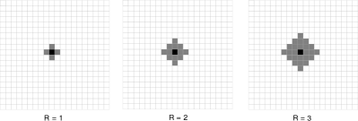
Figure 1: Von Neumann neighborhoods of radius $R=1$, $R=2$, and $R=3$. The focal agent is shown in black and the von Neumann neighborhood for that agent in gray.

Initially, the agents are assigned uniform random culture vectors. The dynamics of the model are as follows. A focal agent $a$ is chosen at random, and another agent $b$ from the radius $R$ von Neumann neighborhood is also chosen at random. With probability proportional to their cultural similarity (the number of features on which they have identical traits), the two agents $a$ and $b$ interact. This interaction results in a randomly chosen feature on $a$ whose value is different from that on $b$ being changed to $b$’s value. This process is repeated until an absorbing, or frozen, state is reached. In this state, no more change is possible, because all agents’ neighbors have either identical or completely distinct (no features in common, so no interaction can occur) culture vectors.

In the absorbing state, the agents form cultural regions, or clusters. Within the cluster, all agents have identical culture vectors. Then the average size of the largest cluster, $\left<S_{\max}\right>/L^{2}$ is used as the order parameter (Castellano et al., 2000; Klemm et al., 2003b; Castellano et al., 2009), separating the ordered and disordered phases. In a monocultural (ordered) state, $\left<S_{\max}\right>/L^{2}\approx 1$, a single cultural region covers almost the entire lattice; in a multicultural (disordered) state, multiple cultural regions exist. Other order parameters that have been used include the number of cultural domains (Axelrod, 1997; Flache and Macy, 2011), mean density of cultural domains (Peres and Fontanari, 2015), entropy (Radillo-Díiaz et al., 2012), overlap between neighboring sites (Klemm et al., 2003c), and activity (number of changes) per agent (Reia and Neves, 2015).

Source code for the model (implemented in C++ and Python with MPI Dalcín et al. (2008)) is available from https://sites.google.com/site/alexdstivala/home/axelrod_qrphase/.

III Results

Figure 2 shows the order parameter (largest region size) plotted against $q$ for $F=5$, on three different lattice sizes. It is apparent that, as the size of the von Neumann neighborhood is increased, the critical value of $q$ also increases. That is, by allowing a larger range of interactions, a larger scope of cultural possibilities is required in order for a multicultural absorbing state to exist. Increasing the lattice size has a similar effect, although, as we shall show in Section IV, there is still a finite critical value of $q$ in the limit of an infinite lattice.

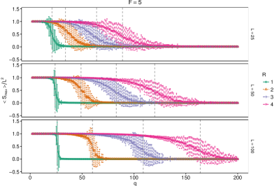
Figure 2: The order parameter $\left<S_{\max}\right>/L^{2}$ (largest region size) plotted against the number of traits $q$ for the Axelrod model for $F=5$, four different values of the von Neumann radius $R$, and three lattice sizes. Each data point is the average over 50 independent runs and error bars show the 95% confidence interval. Vertical dashed lines show the critical value of $q$, where the variance of the order parameter is largest.

Figure 3 shows the order parameter (largest region size) plotted against the von Neumann radius for $F=5$, various values of $q$, and three different lattice sizes. In each case (apart from the smallest value of $q$, in which a monocultural state always prevails), there is a phase transition visible between a multicultural state (for $R$ less than a critical value) and a monocultural state. Note that when $R$ is sufficiently large relative to the lattice size $L$, every agent has every other agent in its von Neumann neighborhood, and hence the situation is equivalent to a complete graph or a well-mixed population (or “soup” (Axtell et al., 1996, p. 132)). In this situation, it has long been known that heterogeneity cannot be sustained (Axtell et al., 1996; Axelrod, 1997). Fig. 3 shows that there appears to be a phase transition controlled by $R$, between the multicultural phase and the monocultural phase. As the size of the neighborhood increases, so does the probability of an agent finding another agent with at least one feature in common with which to interact, and hence local convergence can happen in larger neighborhoods, resulting in larger cultural regions. However this does not result, at the absorbing state (for a fixed value of $q$), in a gradual increase in maximum cultural region size from a completely fragmented state to a monocultural state. Rather, global polarization (a multicultural absorbing state) still occurs for sufficiently small $R$, but at the critical value of the radius $R_{c}$ there is a phase transition so that for neighborhoods defined by $R>R_{c}$ a monocultural state prevails.

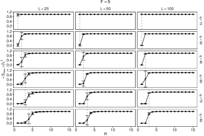
Figure 3: The order parameter $\left<S_{\max}\right>/L^{2}$ (largest region size) plotted against the von Neumann radius $R$ for the Axelrod model for $F=5$, some different values of $q$, and three lattice sizes. Each data point is the average over 50 independent runs and error bars show the 95% confidence interval. Vertical dashed lines show the critical value of $R$, where the variance of the order parameter is largest.

This phase transition is further apparent in Figure 4, which shows histograms of the distribution of the order parameter (largest region size) at the critical radius for some different values of $q$. That is, for each value of $q$, the radius $R_{c}$ at which the variance of the order parameter is greatest. This shows the bistability of the order parameter at the critical radius, where the two extreme values are equally probable (Klemm et al., 2003b).

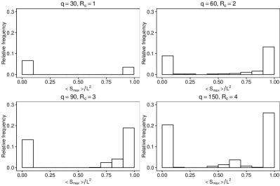
Figure 4: Distribution of the order parameter at the critical radius for some different values of $q$, with $F=5$, $L=100$. Each distribution is from 50 independent runs.

Figure 5 colors points on the $q$ – $R$ plane according to the value of the order parameter, resulting in $q$ – $R$ phase diagram. A multicultural state only results for sufficiently large values of $q$ and small values of $R$. Figure 6 shows the phase transition more clearly, with the multicultural states in the upper left of the plane and the monocultural states in the bottom right.

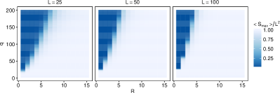
Figure 5: $q$ – $R$ phase diagram showing the order parameter $\left<S_{\max}\right>/L^{2}$ for the Axelrod model for $F=5$ and three lattice sizes ($L=25$, $L=50$, and $L=100$). Each data point is colored according to the size of the largest region $\left<S_{\max}\right>/L^{2}$ averaged over 50 independent runs.

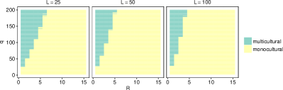
Figure 6: $q$ – $R$ phase diagram for the Axelrod model for $F=5$ and three lattice sizes ($L=25$, $L=50$, and $L=100$). As in Klemm et al. (2003b), the arbitrary, but small, value of 0.1 is used as the value of the order parameter to plot the critical value of $q$ separating the monocultural and multicultural region for each value of the von Neumann neighborhood radius $R$.

IV Mean-field analysis

We detail the mean-field analysis carried out by Castellano et al. (2000) who gave a differential equation. In the mean-field setting, we focus on the bonds between sites (or agents) located on an infinite lattice, so we can assume that each site and its von Neumann neighborhood consists of exactly $g(R)$ sites. The infinite lattice setting naturally implies that we do not consider edge effects.

For a single, randomly chosen bond between two sites, we let $P_{m}(t)$ be the probability that the bond is of type $m$ at time $t$, so both sites of the bond share $m$ common features, while $F-m$ features are different. If the randomly chosen bond is connected to sites $i$ and $j$, then

$$m=\#\{\sigma_{i,f}=\sigma_{j,f}:f\in\{1,\dots,q\}\}.$$

At time $t=0$, we denote by $\rho_{0}$ the probability of a single feature of any two sites being common, so $\rho_{0}=\mathbb{P}(\sigma_{i,f}=\sigma_{j,f})$. If the features are distributed uniformly from $1$ to $q$, then $\rho_{0}=1/q$. It is sometimes assumed that the features have a Poisson distribution (Castellano et al., 2000; Vilone et al., 2002; Barbosa and Fontanari, 2009; Radillo-Díiaz et al., 2012; Peres and Fontanari, 2015) with mean $q$, so then application of the Skellam distribution gives $\rho_{0}=e^{-2q}I_{0}(2q)$, where $I_{0}$ is a modified Bessel function of the first kind. For the single bond, the number of common features is a binomial random variable, so

$$P_{m}(0)=\binom{F}{m}\rho_{0}^{m}(1-\rho_{0})^{F-m}.$$

Castellano et al. (2000) derived a master equation, also known as a forward equation, given by

$$\frac{dP_{m}(t)}{dt}=\sum_{k=1}^{F-1}\frac{k}{F}P_{k}(t)\left[\delta_{m,k+1}-\delta_{m,k}+(g-1)\sum_{n=0}^{F}\left(P_{n}(t)W_{n,m}^{(k)}(t)-P_{m}(t)W_{m,n}^{(k)}(t)\right)\right],$$ (2)

where $W_{n,m}^{(k)}(t)$ is the probability that an $n$-type bond becomes an $m$-type bond due to the updating of a $k$-type neighbor bond (sup, ). This equation is only defined for $1\leq m\leq F$, but naturally the probabilities sum to one, giving

$$P_{0}(t)=1-\sum_{m=1}^{F}P_{m}(t).$$

For $1<m\leq F$, we show (sup, ) that the master equation or, rather, the set of nonlinear differential equations (2) can be re-written as

$$\frac{dP_{m}(t)}{dt}= \left[\frac{m-1}{F}P_{m-1}(t)-\frac{m}{F}P_{m}(t)\right]$$

$$+(g-1)\left[P_{m-1}(t)W_{m-1,m}^{(k)}(t)\right.$$

$$-P_{m}(t)W_{m,m-1}^{(k)}(t)$$

$$+\left.P_{m+1}(t)W_{m+1,m}^{(k)}(t)\right.$$

$$-\left.P_{m}(t)W_{m,m+1}^{(k)}(t)\right]\sum_{k=1}^{F-1}\frac{k}{F}P_{k}(t),$$ (3)

and zeroth differential equation is

$$\frac{dP_{0}(t)}{dt}=-\sum_{m=1}^{F}\frac{dP_{m}(t)}{dt}.$$ (4)

As in Castellano et al. (2000), we can investigate model dynamics within the mean-field treatment by studying the density $n_{a}=\sum_{i=1}^{F-1}P_{i}$ of active bonds, that is a bond across which at least one feature is different and one the same. Hence in an absorbing (frozen) state, $n_{a}=0$. In the mean-field analysis, since an infinite lattice is assumed, $n_{a}=0$ only when a multicultural absorbing state is reached; as noted by Castellano et al. (2000), the coarsening process by which a monocultural state is formed lasts indefinitely on an infinite lattice.

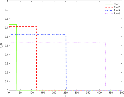
Figure 7: Phase diagram within the mean-field approximation for some different values of the von Neumann radius $R$. The value of $n_{a}(t)$ (shown at $t=10^{3}$) is obtained by numerical integration of (IV) and (4).

Figure 7 plots the number of active bonds against the value of $q$ for some different values of $R$ within the mean-field approximation. It can be seen that the behavior is qualitatively the same as that shown in Fig. 2 for the simulations on finite lattices: the critical value of $q$ is higher for larger neighborhood sizes. On finite lattices, larger lattice sizes also increase the critical value of $q$ for a given neighborhood size, however on an infinite lattice, there is still a finite critical value of $q$ for a given neighborhood size. This suggests that, if the lattice size in the simulation could be increased further (a very computationally demanding process), eventually the critical values would approach those obtained in the mean-field approximation.

V Conclusion

The original Axelrod model had agents only interact with their immediate neighbors on a lattice, modeling the assumption of that geographic proximity largely determines the possibility of interaction. Subsequent work has extended this to neighbors on complex networks, or allowed agent migration, or assumed a well-mixed population (infinite-ranged social interactions) on the assumption that online interactions are making this assumption more realistic (Valori et al., 2012).

Despite these, and other, increasingly sophisticated modifications of the Axelrod model, however, an examination of the consequences of simply extending the lattice (von Neumann) neighborhood had not been carried out. We have done so, and shown another phase transition in the model, controlled by the von Neumann radius $R$, as well as the well-known phase transition at the critical value of $q$, and drawn a $q$ – $R$ phase diagram. We have also used a mean-field analysis to analyze the behavior on an infinite lattice.

These results show that, as well as the value of $q$, the “scope of cultural possibilities” (Axelrod, 1997), having a critical value above which a multicultural state prevails, there is also a critical value of the radius of interaction, above which a monocultural state prevails. This simply says that, rather unsurprisingly, a world in which people can only interact with their immediate neighbors is (for a fixed value of $q$), more likely to remain multicultural than one in which people can interact with those further away. Given this inevitability of a monocultural state for large enough “neighborhoods”, it might be more useful to consider alternative measurements of cultural diversity, such as the “long term cultural diversity” measured using the curve plotting the number of final cultural domains against the initial number of connected cultural components, as the bounded confidence threshold is varied, as described by Valori et al. (2012) (where a well-mixed population was assumed, and hence a monocultural state results for when the bounded confidence threshold is zero). An obvious extension of this work is to examine the behavior of the Axelrod model on complex networks where the neighborhood is extended to all agents within paths of length $R$ on the network.

*