Comoving stars in Gaia DR1:
An abundance of very wide separation comoving pairs

Abstract

The primary sample of the Gaia Data Release 1 is the Tycho-Gaia Astrometric Solution (TGAS): $\approx$ 2 million Tycho-2 sources with improved parallaxes and proper motions relative to the initial catalog. This increased astrometric precision presents an opportunity to find new binary stars and moving groups. We search for high-confidence comoving pairs of stars in TGAS by identifying pairs of stars consistent with having the same 3D velocity using a marginalized likelihood ratio test to discriminate candidate comoving pairs from the field population. Although we perform some visualizations using (bias-corrected) inverse parallax as a point estimate of distance, the likelihood ratio is computed with a probabilistic model that includes the covariances of parallax and proper motions and marginalizes the (unknown) true distances and 3D velocities of the stars. We find 13,085 comoving star pairs among 10,606 unique stars with separations as large as 10 pc (our search limit). Some of these pairs form larger groups through mutual comoving neighbors: many of these pair networks correspond to known open clusters and OB associations, but we also report the discovery of several new comoving groups. Most surprisingly, we find a large number of very wide ($>1$ pc) separation comoving star pairs, the number of which increases with increasing separation and cannot be explained purely by false-positive contamination. Our key result is a catalog of high-confidence comoving pairs of stars in TGAS. We discuss the utility of this catalog for making dynamical inferences about the Galaxy, testing stellar atmosphere models, and validating chemical abundance measurements.

Section 1 Introduction

Stars that are roughly co-located and moving with similar space velocities (“comoving stars”) are of special interest in many branches of astrophysics.

At small separations ($0.001$–$1$ pc), they are wide binaries (and multiples) that are either weakly gravitationally bound or slowly separating. Because they have low binding energies, a sample of wide binaries is valuable for investigating the Galactic dynamical environment. These systems must have both survived their dynamic birth environment and avoided tidal destruction along their orbit. Thus, the statistical properties of wide binaries provide a window into both star formation processes (e.g., Parker et al. 2009) and Galactic dynamics (Heggie 1975), including Galactic tides and other massive perturbers such as molecular clouds and MACHOs (Weinberg et al., 1987; Jiang & Tremaine, 2010; Yoo et al., 2004; Allen & Monroy-Rodríguez, 2014).

Wide binaries are also good test beds for stellar models and age indicators: the constituent stars were likely born at the same time with the same chemical compositions, but evolved independently because of their wide separation. These pairs are therefore useful for validating gyrochronology relations (e.g., Chanamé & Ramírez 2012) and may be valuable for testing consistency between stellar atmosphere models. Finally, calibration of stellar parameters of low-mass stars (e.g., M dwarfs), which dominate the stellar content of the Galaxy by number, can benefit from a larger sample of widely separated binaries containing a low-mass star and a much brighter F/G/K star whose stellar parameters are easier to measure (e.g., Rojas-Ayala et al., 2012).

At larger separations ($\gtrsim 1$ pc), comoving stars are likely members of (potentially dissolving) moving groups, associations, and star clusters or disrupted wide binaries. The origin of moving groups is still under active debate (e.g., Bovy & Hogg 2010): are they remnants of a coeval star formation event with similar chemical composition? Or are they formed by dynamical effects of nonaxisymmetric features of the Galaxy such as spirals and bars? With the recent advances in measuring chemical abundances of a large volume of stars using high- and low- resolution spectroscopy (e.g., Steinmetz et al. 2006; Majewski et al. 2015; Gilmore et al. 2012 to name a few), we can now start to explore these questions with unprecedented statistics and in unexplored detail. The dynamics of cluster dissolution provides important clues to understanding the star formation history and the dynamical evolution of the Milky Way. In the halo, we know of more than 20 disrupting globular clusters and dwarf galaxies (“stellar streams”; see, e.g., Grillmair & Carlin 2016 for a summary of known streams). These tidal streams are modeled to infer the parameters of the Galactic potential (e.g., Küpper et al. 2015). Similar processes are at work with star clusters in the disk. However, the dynamical time is much shorter, and the dynamics will be much more complex because of the existence of other perturbers in the disk.

To date, thousands of candidate comoving star pairs have been identified by searching for stars with common proper motions (Poveda et al. 1994; Allen et al. 2000; Chanamé & Gould 2004; Lépine & Bongiorno 2007; Shaya & Olling 2011; Alonso-Floriano et al. 2015). Here, we use the recent first data release of Gaia which includes precise distances, enabling us to ask whether two stars share the same physical (3D) velocity rather than just the projections in the proper motion space.

This paper proceeds as follows: In Section 2, we briefly describe the data set used in this work. In Section 3, we develop a statistical method to identify high-confidence comoving pairs in this catalog. In Section 4, we present and discuss our resulting catalog of comoving pairs. We summarize in Section 5.

Section 2 Data

The primary data set used in this Article is the Tycho-Gaia Astrometric Solution (TGAS), released as a part of Data Release 1 (DR1) of the Gaia mission (Gaia Collaboration et al., 2016; Lindegren et al., 2016). The TGAS contains astrometric measurements (sky position, parallax, and proper motions) and associated covariance matrices for a large fraction of the Tycho-2 catalog (Høg et al., 2000) with median astrometric precision comparable to that of the Hipparcos catalog ($\approx 0.3~{}{\rm mas}$; van Leeuwen, 2007). In terms of parallax signal-to-noise ($[S/N]_{\varpi}=\varpi/\sigma_{\varpi}$), the TGAS catalog contains 42385 high-precision stars with $[S/N]_{\varpi}>32$.

We construct an initial sample of star pairs to search for comoving pairs as follows. We first apply a global parallax signal-to-noise cut, $[S/N]_{\varpi}>8$, to the TGAS, which leaves 619,618 stars. Then, for each star we establish an initial sample of possible comoving partners by selecting all other stars that satisfy two criteria: separation less than 10 pc and difference in (point-estimate) tangential velocity less than $|\Delta\boldsymbol{v}_{\mathrm{t}}|<10$ $\rm km~{}s^{-1}$. We ultimately build a statistical model that incorporates the covariances of the data, but for these initial cuts and for visualizations we use a point-estimate of the distance by applying a correction for the Lutz-Kelker bias (Lutz & Kelker 1973):

$$\hat{r}=1000\,\left[\frac{\varpi}{2}\,\left(1+\sqrt{1-\frac{16}{[S/N]_{\varpi}^{2}}}\right)\right]^{-1}\,{\rm pc}$$ (1)

where $\varpi$ is the parallax in mas. An estimate for the difference in tangential velocity between two stars is, then,

$$|\Delta\boldsymbol{v}_{\mathrm{t}}|=|\hat{r}_{1}\boldsymbol{\mu}_{1}-\hat{r}_{2}\boldsymbol{\mu}_{2}|$$ (2)

where $\boldsymbol{\mu}=(\mu_{\alpha^{*}},\mu_{\delta})$.

Figure 1 shows $|\Delta\boldsymbol{v}_{\mathrm{t}}|$ against the physical separation for the resulting 271,232 unique pairs in the initial sample. A few key observations can be made:

• At small separations ($<1$ pc), there is a population of pairs with very small tangential velocity difference ($<2$ km/s). Given that these pairs are very close in both 3D position and tangential velocities, it is highly probable that they are actually comoving wide binaries.

• A sample of comoving stars also include stars that are part of, e.g., OB associations, moving groups, and open clusters. These astrophysical objects may be detected as a network of comoving pairs, sharing some mutual comoving neighbors. As the pair separation increases, the nature of comoving pairs will change from binaries to those related to these larger objects, which generally subtend a larger angle in sky. Since the proper motions of two stars with the same 3D velocity are projections of this velocity onto the celestial sphere at two different viewing angles, the larger the difference in viewing angles is, the larger the difference in tangential velocities will be. Due to this projection effect, a population of genuine comoving pairs will extend to larger $|\Delta\boldsymbol{v}_{\mathrm{t}}|$ at larger separation. This indeed can be seen in Figure 1 as an over-density in the lower right corner that gets thinner as $|\Delta\boldsymbol{v}_{\mathrm{t}}|$ increases.

• Finally, there is a population of “random” pairs of field stars that are not comoving, but still have $|\Delta\boldsymbol{v}_{\mathrm{t}}|<10$ $\rm km~{}s^{-1}$ by chance. As $|\Delta\boldsymbol{v}_{\mathrm{t}}|$ increases, this population will dominate. Figure 1 shows that there is an overlap between genuine comoving pairs and “random” pairs.

In the following section, we construct a statistical model that propagates the non-trivial uncertainties in the data to our beliefs about the likelihood that a given pair of stars is comoving.

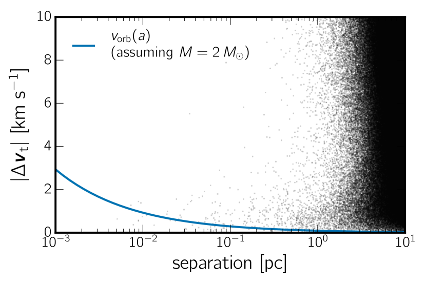
Figure 1: Point estimates of tangential velocity and physical separation computed for all 271,232 unique pairs in the initial sample of pairs (black points). For this sample, we consider stars with separation $<10$ pc and $|\Delta\boldsymbol{v}_{\mathrm{t}}|<10$ $\rm km~{}s^{-1}$ computed relative to every other star in TGAS. The blue solid line shows the magnitude of the 3D orbital velocity as a function of semi-major axis for a $2~{}M_{\odot}$ binary system. Note the stream of points that starts at small separation ($\lesssim 0.01$ pc), small $|\Delta\boldsymbol{v}_{\mathrm{t}}|$ ($\lesssim 2$ $\rm km~{}s^{-1}$), but climbs to larger $|\Delta\boldsymbol{v}_{\mathrm{t}}|$ at $|\Delta\boldsymbol{x}|\gtrsim 1$ pc, which eventually merges with random pairs of field stars dominating in the upper right corner (see Section 2 for details).

Section 3 Methods

The abundance of pairs of stars with small velocity difference in Figure 1 suggests that there are a significant number of comoving pairs in the TGAS data at a range of separations. Here, we develop a method to select high-confidence comoving pairs that properly incorporates the uncertainties associated with the Gaia data. We make the following assumptions in order to construct a statistical model (a likelihood function with explicit priors on our parameters):

• We assume that the uncertainties in the data—parallax, $\varpi$, and two proper motion components, $\boldsymbol{\mu}={(\mu_{\alpha^{*}}\,\mu_{\delta})}^{\!\mathsf{T}}$ —are Gaussian with known covariances $\mathbf{C}$. The values of covariances are provided as part of the Gaia data (Lindegren et al., 2012, 2016).

• We assume that the 3D velocities of stars in a given pair $(\boldsymbol{v}_{i},\boldsymbol{v}_{j})$ (relative to the solar system barycenter) are either (1) the same with a small (Gaussian) dispersion $s$ or (2) independent. In both cases, velocity is drawn from the velocity prior $p(\boldsymbol{v})$.

Under these assumptions, the likelihood of a proper motion measurement, $\boldsymbol{\mu}$, for a star with true distance, $r$, and true 3D velocity $\boldsymbol{v}$ is

$$L(\boldsymbol{\mu}\,|\,\boldsymbol{v},r,s^{2}) =\left[\det\left(\frac{\tilde{\mathbf{C}}^{-1}}{2\pi}\right)\right]^{1/2}\,\exp\left[-\frac{1}{2}{\left(\boldsymbol{\mu}-\boldsymbol{x}_{\theta}\right)}^{\!\mathsf{T}}\,\tilde{\mathbf{C}}^{-1}\,\left(\boldsymbol{\mu}-\boldsymbol{x}_{\theta}\right)\right]$$ (3)

$$\boldsymbol{x}_{\theta} =r^{-1}\,\boldsymbol{v}_{t}$$ (4)

where the tangential velocity $\boldsymbol{v}_{t}=(\begin{array}[t]{c c}v_{\alpha}&v_{\delta}\end{array})^{\mathsf{T}}$ is related to the 3D velocity $\boldsymbol{v}$ by projection matrix $\mathbf{M}$ at the star’s sky position $(\alpha,\delta)$

$$\boldsymbol{v}_{t} =\mathbf{M}\,\boldsymbol{v}$$ (5)

$$=\left(\begin{array}[]{c c c}-\sin\alpha&\cos\alpha&0\\ -\sin\delta\,\cos\alpha&-\sin\delta\,\sin\alpha&\cos\delta\end{array}\right)\,\left(\begin{array}[]{c}v_{x}\\ v_{y}\\ v_{z}\end{array}\right)$$ (11)

and the modified covariance matrix $\tilde{\mathbf{C}}$ is

$$\tilde{\mathbf{C}}=\mathbf{C}+(s/r)^{2}\,\mathbb{I}$$ (12)

where $\mathbb{I}$ is the identity matrix. The parameter $s$ is added to allow for small tolerance in velocities which we discuss below.

For a given pair, we compute the fully marginalized likelihood (FML) for the hypotheses (1) and (2), $\mathcal{L}_{1}$ and $\mathcal{L}_{2}$. We use the FML ratio $\mathcal{L}_{1}/\mathcal{L}_{2}$ as the scalar quantity to select candidate comoving pairs, as described in $Section~{}\ref{sub:selection}$ in more detail. To compute these FMLs, the likelihood functions for each star in a pair, $L_{i},L_{j}$, are marginalized over the (unknown) true distance and 3D velocity for each star in the pair $(i,j)$.

$$\mathcal{L}_{1} =\int\,\mathrm{d}r_{i}\,\mathrm{d}r_{j}\,\mathrm{d}^{3}\boldsymbol{v}\,L_{i}(\boldsymbol{\mu_{i}}\,|\,\boldsymbol{v},r_{i},s^{2})\,L_{j}(\boldsymbol{\mu_{j}}\,|\,\boldsymbol{v},r_{j},s^{2})\,p(\boldsymbol{v})\,p(r_{i}\,|\,\varpi_{i})\,p(r_{j}\,|\,\varpi_{j})$$ (13)

$$\mathcal{L}_{2} =\int\,\mathrm{d}r_{i}\,\mathrm{d}r_{j}\,\mathrm{d}^{3}\boldsymbol{v}_{i}\,\mathrm{d}^{3}\boldsymbol{v}_{j}\,L_{i}(\boldsymbol{\mu_{i}}\,|\,\boldsymbol{v}_{i},r_{i},s^{2})\,L_{j}(\boldsymbol{\mu_{j}}\,|\,\boldsymbol{v}_{j},r_{j},s^{2})\,p(\boldsymbol{v}_{i})\,p(\boldsymbol{v}_{j})\,p(r_{i}\,|\,\varpi_{i})\,p(r_{j}\,|\,\varpi_{j}).$$ (14)

Here, $p(r_{i}\,|\,\varpi_{i})$ is the posterior distribution of distance given parallax measurement $\varpi_{i}$ and its Gaussian error $\sigma_{\varpi,i}$. Note that the FML for the hypothesis (1) involves integration over one velocity $\boldsymbol{v}$ that generates the likelihoods for both stars, $L_{i}$ and $L_{j}$. The marginalization integral for hypothesis (2) can be split into the product of two simpler integrals $\mathcal{L}_{2}=Q(\boldsymbol{\mu_{i}},\varpi_{i})\,Q(\boldsymbol{\mu_{j}},\varpi_{j})$ where

$$Q(\boldsymbol{\mu},\varpi)=\int\,\mathrm{d}r\,\mathrm{d}^{3}\boldsymbol{v}\,L(\boldsymbol{\mu}\,|\,\boldsymbol{v},r,s^{2})\,p(\boldsymbol{v})\,p(r\,|\,\varpi)$$ (15)

If the velocity prior $p(\boldsymbol{v})$ is also Gaussian, the integrals over velocity in both cases can be performed analytically: We use a mixture of three isotropic, zero-mean Gaussian distributions

$$p(\boldsymbol{v})=\sum_{m=1}^{3}\,w_{m}\,\mathcal{N}(0,\sigma_{v,m}^{2})$$ (16)

with velocity dispersions $(\sigma_{v,1},\sigma_{v,2},\sigma_{v,3})=(15,30,50)~{}\rm km~{}s^{-1}$ and weights $(w_{1},w_{2},w_{3})=(0.3,0.55,0.15)$ meant to encompass young thin disk stars to halo stars. These numbers are empirically chosen to account for the distribution of velocities of the TGAS stars. We derive the relevant expressions in Appendix B. After marginalizing over velocity, the likelihood integrands only depend on distance; we numerically compute the integrals over the true distances of each star in a pair using Monte Carlo integration with $K$ samples from the distance posterior.

$$\int\,\mathrm{d}r\,\tilde{L}(r)\,p(r\,|\,\varpi)\approx\frac{1}{K}\,\sum_{k}^{K}\,\tilde{L}(r_{k})$$ (17)

where $\tilde{L}(r)$ is the velocity-marginalized likelihood function. In order to generate a sample of distances from the distance posterior $p(r_{i}\,|\,\varpi_{i})$, we need to assume a distance prior. We adopt the uniform density prior (Bailer-Jones, 2015) with a maximum distance of 1 kpc. Through experimentation, we have found that $K=128$ samples are sufficient for estimating the above integrals for stars with a wide range in parallax signal-to-noise.

For small-separation binaries, the assumption that the stars having the same 3D velocity for hypothesis (1) can break down for high-precision proper motion measurements because of the orbital velocity (blue solid line in Figure 1). To account for this, we set $s^{2}=\frac{2\,G\,{\rm M}_{\odot}}{|\boldsymbol{x}_{i}-\boldsymbol{x}_{j}|}$. Because $s^{2}$ is much smaller than the velocity dispersions of the velocity prior $p(\boldsymbol{v})$, it has minimal effect on the hypothesis (2) FML.

Section 4 Results

This section is divided into three parts. First, we discuss and justify a cut of the likelihood ratio to select candidate comoving pairs. Second, we present the statistics and properties of our candidate comoving pairs. Finally, we describe our catalog of candidate comoving pairs, the main product of this study.

4.1 Selecting candidate comoving pairs

In this section, we examine the distribution of (log-)likelihood ratios $\ln\mathcal{L}_{1}/\mathcal{L}_{2}$, and come up with a reasonable cut for this quantity to select comoving pairs from the initial sample.

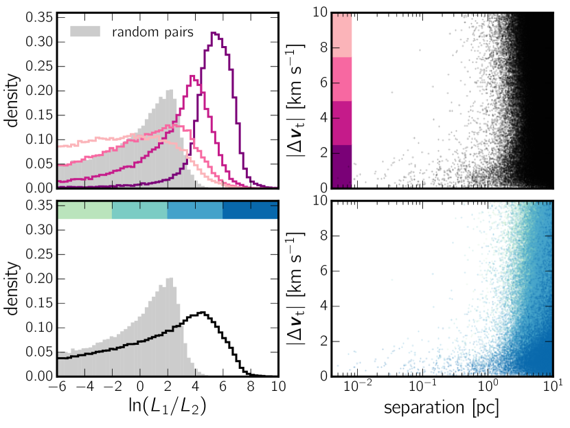
Figure 2: Justification of the likelihood ratio cut. On the top row, we show how the distribution of $\ln\mathcal{L}_{1}/\mathcal{L}_{2}$ changes (left) in slices of $|\Delta\boldsymbol{v}_{\mathrm{t}}|$ (sequentially color-coded in pink on the right panel). On the bottom row, we show how the distribution of pairs on $|\Delta\boldsymbol{v}_{\mathrm{t}}|$ vs. separation changes (right) in slices of $\ln\mathcal{L}_{1}/\mathcal{L}_{2}$ (sequentially color-coded in blue on the left). The black dots in the upper right panel and the black line in the lower left panel correspond to the entire initial sample of pairs. For comparison, we also present the likelihood ratio distribution of random pairs of stars in the TGAS with parallax $S/N>8$ in gray filled histogram. Based on this, we choose $\ln\mathcal{L}_{1}/\mathcal{L}_{2}>6$ as our high-confidence candidate comoving pairs.

Figure 2 shows the likelihood ratios for all $\sim 271$k pairs in the initial sample. As discussed in Section 2, we expect a correlation between the likelihood ratios of pairs, and their distribution on $|\Delta\boldsymbol{v}_{\mathrm{t}}|$ vs separation plane. Specifically, as we sweep through from small $|\Delta\boldsymbol{v}_{\mathrm{t}}|$ to large, we expect the population of pairs to change from genuinely comoving to random. This becomes clear when we look at the distribution of the likelihood ratios of pairs in slices of $|\Delta\boldsymbol{v}_{\mathrm{t}}|$ (top row of Figure 2). Pairs with $|\Delta\boldsymbol{v}_{\mathrm{t}}|\in(0,2.5)~{}\rm km~{}s^{-1}$ are most likely actual comoving pairs, and their likelihood ratio distribution is narrowly peaked at $\gtrsim 5$ (darkest pink histogram in the upper left panel of Figure 2). The distribution peaks at lower values and gets broader as $|\Delta\boldsymbol{v}_{\mathrm{t}}|$ increases, and the number of random pairs increasingly dominate. On the bottom row of Figure 2, we show how the distribution of pairs on $|\Delta\boldsymbol{v}_{\mathrm{t}}|$ vs separation plane changes with decreasing $\ln\mathcal{L}_{1}/\mathcal{L}_{2}$ ratios. This is in agreement with our discussion in Section 2. Finally, as a test, we compute the likelihood ratios for 200,000 random pairs of stars with the same parallax signal-to-noise ratio cut as the initial sample ($S/N>8$). Shown as the gray filled histogram in Figure 2, this distribution peaks at a much lower value ($\approx 2$), and is clearly separated from highly probable comoving pairs.

Based on these comparisons, we select candidate comoving pairs with $\ln\mathcal{L}_{1}/\mathcal{L}_{2}>6$. Out of 271,232 pairs in the initial sample, 13,058 pairs (4.8%) satisfy this condition.

4.2 Statistics and properties of the identified comoving pairs

Figure 3: Histogram of the sizes of connected components.

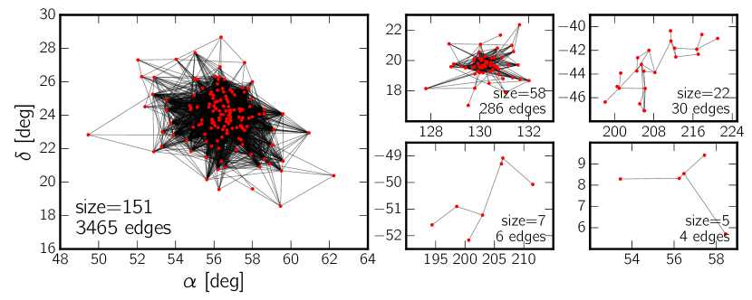
Figure 4: Visualizations of a few example connected components of comoving pairs of stars. Each star (node) is marked as a red circle, and a line (edge) is drawn between two stars if they are comoving by our selection criteria (see Section 4.1). On left, we show the largest network found in this study corresponding to the Pleiades star cluster. On right, we show four examples of connected components with varying sizes. The connected component on the upper left panel with a size of 58 corresponds to NGC 2632, also known as the Beehive cluster.

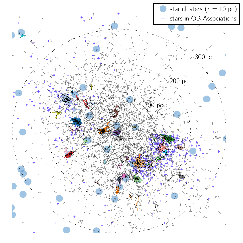
Figure 5: Panoramic view of comoving pairs of stars around the Sun. This is a cylindrical projection of onto the Galactic plane with the Sun at the origin. Pairs in connected components of sizes less than 5 are connected by gray lines. Pair in connected components of size $\geq 5$ are plotted with a unique random color, and their nodes (stars) are highlighted with small black circles. We also show the positions of known Milky Way star clusters from Kharchenko et al. (2016) as light blue circles of $10$ pc radius, and stars in OB associations from de Zeeuw et al. (1999) as blue crosses. Some of the larger connected components are clearly associated with known clusters, but we also discover quite a few new comoving groups.

Once we have identified candidate comoving pairs from the initial sample, these pairs form an undirected graph where stars are nodes, and edges between the nodes exist for comoving pairs of stars. A star may have multiple comoving neighbors, and two stars may either be directly or indirectly connected by a sequence of edges (“path”). We divide the graph into connected components, and show the distribution of their sizes in Figure 3. The most common are connected components of size 2, which mean mutually exclusive comoving pairs. However, it is clear that there are many aggregates of comoving stars discovered by looking for comoving pairs. These aggregates are likely moving groups, OB associations, or star clusters. In 13,058 comoving pairs that we identified, there are 4,555 connected components among 10,606 unique stars. The maximum size of the connected components is 151. We show this largest connected component along with four other examples of varying sizes in Figure 4. The largest connected component corresponds to the Pleiades open cluster (left panel of Figure 4) while the upper left panel of the right column of Figure 4 is NGC 2632, another known Milky Way open cluster (Kharchenko et al., 2016).

We show the distribution of comoving pairs in galactic longitude and distance in Figure 5. The connection between known comoving structures and the larger connected components found in this work becomes immediately clear when we overplot the positions of known Milky Way star clusters (Kharchenko et al., 2016), and stars in OB associations (de Zeeuw et al., 1999). Many of the larger connected components are clearly associated with known star clusters: Melotte 22 (Pleiades) at $(l,d)\approx(167\arcdeg,130~{}\textrm{pc})$, Melotte 20 at $(l,d)\approx(147\arcdeg,175~{}\textrm{pc})$, Melotte 25 (Hyades) at $(l,d)\approx(180\arcdeg,50~{}\textrm{pc})$, and NGC 2632 (Beehive) at $(l,d)\approx(206\arcdeg,187~{}\textrm{pc})$ to name a few. Clumps of comoving pairs at $(l,d)\approx(300-360\arcdeg,100-200~{}\textrm{pc})$ seem to strongly correlate with the locations of OB associations Upper Scorpius, Upper Centaurus Lupus, and Lower Centaurus Crux (de Zeeuw et al., 1999).

However, there are still many new larger connected components that we discover. If we define a condition to associate a connected component to a known cluster as having more than 3 members within 10 pc from the nominal position of the cluster, for the 61 connected components with sizes larger than 5, we find that only 10 are associated with a cluster cataloged in Kharchenko et al. (2016). It is also worth noting that the positions of some of the known clusters are offset from those of the connected components associated with them, indicating that the TGAS data improves the distance estimates of these clusters. Finally, not all known star clusters are recovered in our search. This is primarily because of the non-uniform coverage and magnitude limit of the TGAS data.

Ultimately, any candidate comoving pair found in this work needs to be verified using radial velocities. Here, we use 210,368 cross-matches of the TGAS with Radial Velocity Experiment fifth data release (RAVE DR 5; Kunder et al. 2017) to assess the false-positive rates of our selection. We have 283 pairs with both stars matched with RAVE. Figure 6 shows the difference in radial velocities between the two stars in a pair, $\Delta v_{r}$, as a function of their physical separation. We show $\Delta v_{r}$ in units of $\sigma_{\Delta v_{r}}$ which we estimate as the quadrature sum of $\sigma_{v_{r}}$ for each star. The fraction of pairs with good agreement in radial velocity decreases with increasing separation. This, after all, is not surprising because we are only using 2D velocity information (proper motions) with errors. However, the contamination becomes significant only at $>1$ pc (which depends on the local stellar number density and velocity dispersion). Given the excellent correspondence between aggregates of comoving pairs (connected components) and known genuine comoving structures (Figure 5), we may expect that pairs in these larger connected components, which will often have separations $>1$ pc, to have less contamination from false-positives. We divide the comoving pairs into those mutually exclusively connected (i.e., in a connected component of size 2), and those in a larger group. We indeed find that many pairs in larger groups are at $>1$ pc, yet the fraction of pairs that have identical radial velocities within $3\sigma$ is higher than the mutually exclusive pairs, and remains high ($>80\%$) to $\sim 10$ pc. Finally, we note that the false-positive rate for mutually exclusive pairs with large angular separation may have been over-estimated due to projection.

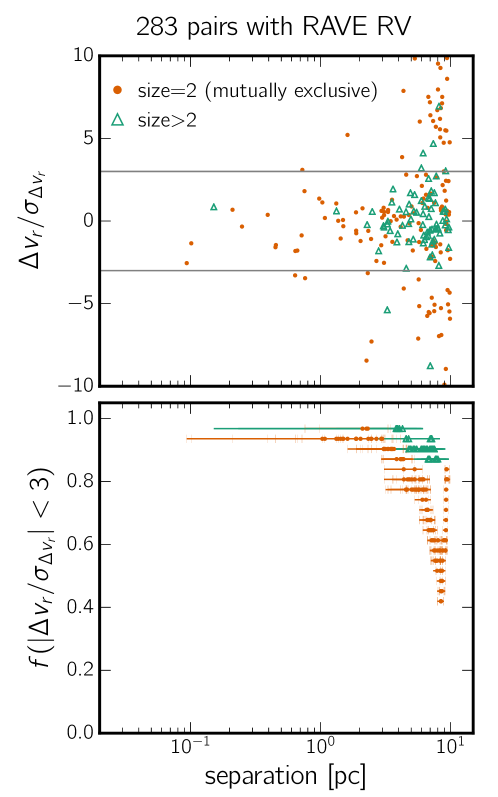
Figure 6: Validation of candidate comoving pairs using radial velocities from RAVE. Top: Radial velocity differences, $\Delta v_{r}$, of 283 pairs with RAVE measurements. $\Delta v_{r}$ is plotted in units of $\sigma_{\Delta v_{r}}=\sqrt{\sigma_{v_{r},1}^{2}+\sigma_{v_{r},2}^{2}}$ as a function of physical separation. We highlight $3\sigma$ limit with two horizontal lines. Bottom: Fraction of pairs with $|\Delta v_{r}/\sigma_{\Delta v_{r}}|<3$ as a function of physical separation. We calculate the fraction with a running bin containing 31 data points at a time. The median, and the minimum and maximum separation of pairs in each bin are indicated with a marker, and its errorbars. We separate pairs in connected components of size 2 (i.e., mutually exclusively connected) from those in larger connected components.

We now examine the separation distribution of comoving pairs in Figure 7. As expected, pairs in larger connected components are mostly found with separations larger than 1 pc. Surprisingly, however, we also find a large number of mutually exclusive comoving pairs at $>1$ pc as well. Even if we consider the increasing false-positive rate at large separations, the distribution is not significantly changed as the number of pairs at $>1$ pc is in fact increasing much faster (as a power-law) than the decrease due to the false-positives (bottom panel of Figure 6). The nature of these very wide separation, mutually exclusive pairs, which cannot be gravitationally bound to each other, needs further investigation. Can they be remnants of escaped binaries that are drifting apart? In a study of the evolution of wide binaries including the Galactic tidal field as well as passing field stars, Jiang & Tremaine (2010) found that we expect to find a peak at $\sim 100-300$ pc in the projected separation due to stars that were once in a wide binary system, but are drifting apart with small relative velocities ($\sim 0.1$ $\rm km~{}s^{-1}$). In future work, we will increase the maximum search limit (in this work, 10 pc) to identify and study these large scale phase-space correlations.

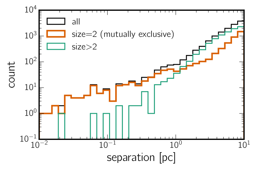
Figure 7: Separation distribution of comoving pairs of stars. As with Figure 6, we divide the pairs into those mutually exclusively connected (connected component size $=2$), and those connected to larger connected components (size $>2$).

Finally, we present the color-magnitude diagrams of comoving pairs using the cross-matches with 2MASS. A more detailed study of stellar parameters using photometry from various sources will follow. Figure 8 and 9 shows $G-J$ vs $G$ color-magnitude diagrams for stars in larger connected components (size$>2$) and in mutually exclusive pairs, respectively. The connected components shown in Figure 8 correspond to those visualized in Figure 4. For stars in larger comoving groups, there is a noticeable lack of evolved, off-main sequence stars, in agreement with these kinematic structures being young. For mutually exclusive pairs, we divide the pairs by separation at 1 pc above which the false-positive rate due to random pairs starts to increase. While many pairs are located along the main sequence, we also find quite a few of main sequence-red giant pairs, which will be valuable to anchoring stellar atmospheric models together.

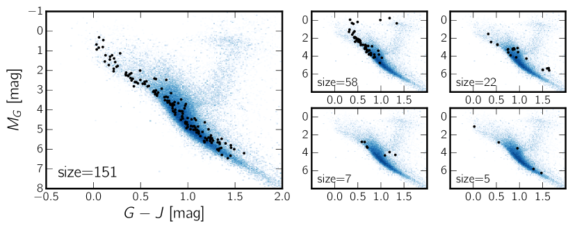
Figure 8: Color-magnitude diagrams of stars in larger connected components presented in Figure 4. Each panel shows the same group of stars visualized in the panel at the same position in Figure 4. We show a reference distribution of stars randomly drawn to have a matching distribution in distance as the stars in our comoving pairs in blue.

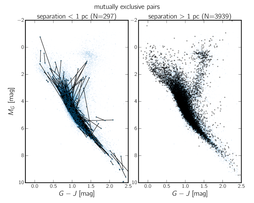
Figure 9: Color-magnitude diagrams of stars in mutually exclusive comoving pairs in two separation bins. We connect each pair by a line on the left for pairs with separations smaller than 1 pc. We show a reference distribution of stars randomly drawn to have a matching distribution in distance as the stars in our comoving pairs in blue, same as Figure 8.

4.3 Catalog of candidate comoving pairs

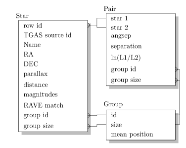
Figure 10: Schematic diagram of the relationship between the tables. See Section 4.3 and Table 1 for details.

Table 1: Candidate co-moving pairs catalog description

Column Name	Unit	Description
Table: Star (10,606 rows)
row id		Zero-based row index
TGAS source id		Unique source id from TGAS
Name		Hipparcos or Tycho-2 identifier
RA	deg	Right ascension from TGAS
DEC	deg	Declination from TGAS
parallax	mas	Unique source id from TGAS
distance	pc	Unique source id from TGAS
$G$	mag	Gaia $G$-band magnitudes
$J$	mag	2MASS $J$-band magnitudes
RAVE OBS ID		Unique id of the RAVE match
RV	$\rm km~{}s^{-1}$	Radial velocity from RAVE
eRV	$\rm km~{}s^{-1}$	Uncertainty of radial velocity from RAVE
group id		Id of the group this star belongs to
group size		Size of the group this star belongs to
Table: Pair (13,058 rows)
star 1		Index of star 1 in the star table
star 2		Index of star 2 in the star table
angsep	arcmin	Angular separation
separation	pc	Physical separation
$\ln\mathcal{L}_{1}/\mathcal{L}_{2}$		Likelihood ratio
group id		Id of the group the pair belongs to
group size		Size of the group the pair belongs to
Table: Group (4,555 rows)
id		Unique group id
size		Number of stars in a group
mean RA	deg	Mean right ascension of members
mean DEC	deg	Mean declination of members
mean distance	pc	Mean distance of members

In this section, we describe our catalog of candidate comoving pairs of stars. The catalog is composed of three tables of stars, pairs, and groups. We summarize the content of each table in Table 1, and the relationships between the tables in Figure 10. The star table contains all 10,606 stars that have at least one comoving neighbor by our selection. We provide the TGAS source id, which may be used to easily retrieve cross matches between Gaia and other surveys using the Gaia data archive. For each star, we also include the positional measurements from TGAS, Gaia $G$-band, 2MASS $J$-band magnitudes, and RAVE radial velocities where they exist. The comoving relationship between the stars is described in the pair table. We also list the angular and physical separation of each pair, and the likelihood ratio, $\ln\mathcal{L}_{1}/\mathcal{L}_{2}(>6)$ (see Equation 13 and 14) computed in this work.

Finally, the information about the connected components found in these comoving star pairs is in the group table. We assign a unique index to each group in descending order of its size. Thus, group 0 is the largest group that contains 151 stars. Each star or pair is associated with a group that it is a member of, listed in the group id column of the star and pair table.

We note a caveat on the completeness of a connected component of comoving pairs found in our catalog. Because we applied a simple cut in the likelihood ratio ($\ln\mathcal{L}_{1}/\mathcal{L}_{2}>6$), there is a possibility that, for example, a star in a mutually exclusive pair in our catalog may still have another possibly comoving companion which has been dropped because the likelihood ratio is slightly less than 6.

Section 5 Summary

In this Article, we searched for comoving pairs of stars in the TGAS catalog released as part of the Gaia DR1. Our method is to compare the fully marginalized likelihoods between two hypotheses: (1) that a pair of stars shares the same 3D velocity, and (2) that the two stars have independent 3D velocities, in both cases incorporating the covariances of parallax and proper motions. We argued for a reasonable cut of the likelihood ratio, and found 13,058 candidate comoving pairs among 10,606 stars with separations ranging from 0.005 pc to 10 pc, the limit of our search.

We found that some comoving pairs that we have identified are connected by sharing a common comoving neighbor. This network of comoving pairs, which forms an undirected graph, can be decomposed into connected components in which any two stars are connected by a path. The entire 13,058 candidate comoving pairs are grouped into 4,555 connected components. The most common is a size-2 connected component, i.e., the two stars in these pairs are mutually exclusively linked. Many of the larger connected components naturally correspond to some of the known comoving structures such as open clusters and stellar associations. Some of these comoving groups of stars are newly discovered.

We have also found a large number of very wide separation ($>1$ pc) mutually exclusive comoving pairs, in which the stars are the only comoving neighbor of each other and not part of large connected components. These are most likely remnants of dissolving wide binaries (Jiang & Tremaine 2010). The abundance of highly probable wide separation comoving pairs conclusively shows that there is no strict cut-off semi-major axis for wide binary systems (e.g., Wasserman & Weinberg 1987). The presence of these pairs and similar separation distribution have already been noticed by Shaya & Olling 2011 using the Hipparcos data. If confirmed with radial velocity measurements, this population should still be relatively young compared to the general disk field population. Modeling the color-magnitude diagram distribution of these stars can shed some light on this issue. If they are remnants of dissolving systems that were born coeval, the sample of very wide separation comoving pairs can potentially be used to measure the recent ($\lesssim 1$ Gyr) star formation history in the Solar neighborhood. Comoving stars with separation less than 1 pc are very promising candidates for wide binaries. They are found to be pairs of stars of varying stellar types. Some of these pairs, such as main sequence-red giant or F/G/K-M dwarfs, will be particularly valuable for testing theoretical stellar models and calibrating observational measurements of low mass stars.

We note that a similar search for wide binaries using the TGAS data is performed in a recent work by Oelkers et al. (2016). They find $\approx$1,900 wide binaries with separation typically less than 1.5 pc, and 256 pairs with separation larger than $\sim 1$ pc. We emphasize that our method is based on a probabilistic model for the assumptions on the 3D velocities of the two stars in a pair, and that we marginalize over the (unknown) true distances and velocities of the stars in contrast to just applying a cut in the proper motion space.

Finally, we make our catalog of 13,058 candidate comoving pairs available to the community. What we find using the TGAS is only a taste of what we will discover with the future releases of the Gaia mission.

Appendix A Relevant properties of Gaussian integrals

In what follows, all vectors are column vectors, unless we have transposed them. A relevant exponential integral solution is

$$\ln\left[\int\exp(-\frac{1}{2}\,{[\boldsymbol{x}-\boldsymbol{\nu}]}^{\!\mathsf{T}}\,{\mathbf{A}}^{-1}\,[\boldsymbol{x}-\boldsymbol{\nu}]-\Delta)\,\mathrm{d}\boldsymbol{x}\right] = +\frac{1}{2}\ln||2\pi\,\mathbf{A}||-\Delta\quad,$$ (A1)

where $\boldsymbol{x}$ and $\boldsymbol{\nu}$ are $D$-dimensional vectors, $\mathbf{A}$ is a positive definite matrix, $\Delta$ is a scalar, and the integral is over all of $D$-dimensional $\boldsymbol{x}$-space. To cast our problem in this form, we will need to complete the square of the exponential argument. If we equate

$$\frac{1}{2}\,{[\boldsymbol{x}-\boldsymbol{\nu}]}^{\!\mathsf{T}}\,{\mathbf{A}}^{-1}\,[\boldsymbol{x}-\boldsymbol{\nu}]+\Delta = \frac{1}{2}\,{\boldsymbol{x}}^{\!\mathsf{T}}\,{\mathbf{A}}^{-1}\,\boldsymbol{x}+{\boldsymbol{x}}^{\!\mathsf{T}}\,\mathbf{B}\,\boldsymbol{b}+C\quad,$$ (A2)

where $\mathbf{B}\,\boldsymbol{b}$ is a $D$-vector, and $C$ is a scalar, then we find

$$\boldsymbol{\nu} = -\mathbf{A}\,\mathbf{B}\,\boldsymbol{b}$$ (A3)

$$\Delta = C-\frac{1}{2}\,{\boldsymbol{\nu}}^{\!\mathsf{T}}\,{\mathbf{A}}^{-1}\,\boldsymbol{\nu}\quad.$$ (A4)

We will identify terms in our likelihood functions with $\mathbf{A}$, $\mathbf{B}\,\boldsymbol{b}$, and $C$, convert to $\boldsymbol{\nu}$ and $\Delta$ and compute the marginalized likelihood using Equation A1.

Appendix B Expressions for the marginalized likelihoods

At given distance $r$, the velocity-marginalized likelihood can be computed analytically using the expressions in Appendix A. We will start by writing down expressions for the the likelihood multiplied by the prior pdf for the velocities. The likelihood for the data (proper motions of the two stars in a pair) is a Gaussian (Equation 3). In order to simplify our notation, we construct a velocity-space data vector $\boldsymbol{y}$ as follows:

$$\boldsymbol{y}={\left(\begin{array}[]{c c c c}r_{i}\,\mu_{\alpha,i}^{*}&r_{i}\,\mu_{\delta,i}&r_{j}\,\mu_{\alpha,j}^{*}&r_{j}\,\mu_{\delta,j}\end{array}\right)}^{\!\mathsf{T}}$$ (B1)

where the subscripts $i,j$ refer to the indices of each star in the pair and we have multiplied the observables (the proper motions) by the distances $r_{i},r_{j}$, which is permitted because we are conditioning on the distances. Fundamentally, our hypothesis 1 model (the stars have the same velocity with a small difference) is

$$\boldsymbol{y}=\mathbf{M}\,\boldsymbol{v}+\mathrm{noise}$$ (B2)

where now the $4\times 3$ transformation matrix $\mathbf{M}$ is a stack of the transformation matrices for each star computed from the pair of sky positions and using Equation 11. The noise (in $\boldsymbol{y}$) is drawn from a $4\times 4$ Gaussian with block-diagonal covariance matrix, $\mathbf{\Sigma}$, constructed from the proper motion covariance matrix of each star, $\mathbf{C}_{i},\mathbf{C}_{j}$, and the distances $r_{i},r_{j}$:

$$\mathbf{\Sigma}=\left(\begin{array}[]{c c}r_{i}^{2}\,\mathbf{C}_{i}&0\\ 0&r_{j}^{2}\,\mathbf{C}_{j}\end{array}\right)$$ (B3)

Given these definitions, the likelihood function for hypothesis 1 is

$$p(\mathrm{data}\,|\,\boldsymbol{v},r_{i},r_{j}) = r_{i}^{2}\,r_{j}^{2}\,{\mathcal{N}}(\boldsymbol{y}\,|\,\mathbf{M}\,\boldsymbol{v},\mathbf{\Sigma})$$ (B4)

$$\ln p(\mathrm{data}\,|\,\boldsymbol{v},r_{i},r_{j}) = 2\,\ln r_{i}+2\,\ln r_{j}-\frac{1}{2}\,\ln||2\pi\,\mathbf{\Sigma}||$$ (B5)

$$\quad-\frac{1}{2}\,{[\boldsymbol{y}-\mathbf{M}\,\boldsymbol{v}]}^{\!\mathsf{T}}\,{\mathbf{\Sigma}}^{-1}\,[\boldsymbol{y}-\mathbf{M}\,\boldsymbol{v}]\quad,$$

where the factor of $r_{i}^{2}\,r_{j}^{2}$ is the Jacobian of the transformation from $\boldsymbol{y}$ to the data space (${(\mu_{\alpha,i}^{*}\ \,\mu_{\delta,i}\ \,\mu_{\alpha,j}^{*}\ \,\mu_{\delta,j})}^{\!\mathsf{T}}$).

Now we multiply this likelihood with the velocity prior. As described in Section 3 we use an isotropic, mixture-of-Gaussians prior on velocity (Equation 16). For simplicity here let us work out the marginalization for one component of the mixture so that $\boldsymbol{v}\sim{\mathcal{N}}(\boldsymbol{0},\mathbf{V}_{m})$. Then,

$$\ln p(\boldsymbol{v})=-\frac{1}{2}\,\ln||2\pi\,\mathbf{V}_{m}||-\frac{1}{2}{\boldsymbol{v}}^{\!\mathsf{T}}\,{\mathbf{V}_{m}}^{-1}\,\boldsymbol{v}$$ (B6)

We can identify $\boldsymbol{\nu}$ and $\Delta$ in $\ln p(\boldsymbol{v})+\ln p(\mathrm{data}\,|\,\boldsymbol{v},r_{i},r_{j})$ using Equation A3 and A4 as

$$\mathbf{A} = {[{\mathbf{M}}^{\!\mathsf{T}}\,{\mathbf{\Sigma}}^{-1}\,\mathbf{M}+{\mathbf{V}_{m}}^{-1}]}^{-1}$$ (B7)

$$\boldsymbol{\nu} = -\mathbf{A}\,{\mathbf{M}}^{\!\mathsf{T}}\,{\mathbf{\Sigma}}^{-1}\,\boldsymbol{y}$$ (B8)

$$\Delta = -2\,\ln r_{i}-2\,\ln r_{j}+\frac{1}{2}\,\ln||2\pi\,\mathbf{\Sigma}||+\frac{1}{2}\,\ln||2\pi\,\mathbf{V}_{m}||$$ (B9)

$$\quad+\frac{1}{2}\,{\boldsymbol{y}}^{\!\mathsf{T}}\,{\mathbf{\Sigma}}^{-1}\,\boldsymbol{y}-\frac{1}{2}\,{\boldsymbol{\nu}}^{\!\mathsf{T}}\,{\mathbf{A}}^{-1}\,\boldsymbol{\nu}\quad,$$

which we plug in to Equation A1 to get the marginalized likelihood conditioned on the two distances $r_{i},r_{j}$.

The marginalized likelihood for the hypothesis 2 model (the stars have independent velocities) is very similar. In this case, the marginalized likelihood is a product of two independent integrals $Q$, composed in the same way as the hypothesis 1 model but now for each star individually, where

$$\boldsymbol{y} = {\left(\begin{array}[]{c c}r\,\mu_{\alpha}^{*}&\quad r\,\mu_{\delta}\end{array}\right)}^{\!\mathsf{T}}$$ (B11)

$$\mathbf{\Sigma} = r^{2}\,\mathbf{C}$$ (B12)

and $\mathbf{M}$ is now the transformation matrix for one star. Then,

$$\mathbf{A} = {[{\mathbf{M}}^{\!\mathsf{T}}\,{\mathbf{\Sigma}}^{-1}\,\mathbf{M}+{\mathbf{V}_{m}}^{-1}]}^{-1}$$ (B14)

$$\boldsymbol{\nu} = -\mathbf{A}\,{\mathbf{M}}^{\!\mathsf{T}}\,{\mathbf{\Sigma}}^{-1}\,\boldsymbol{y}$$ (B15)

$$\Delta = -2\,\ln r+\frac{1}{2}\,\ln||2\pi\,\mathbf{\Sigma}||+\frac{1}{2}\,\ln||2\pi\,\mathbf{V}_{m}||$$ (B16)

$$\quad+\frac{1}{2}\,{\boldsymbol{y}}^{\!\mathsf{T}}\,{\mathbf{\Sigma}}^{-1}\,\boldsymbol{y}-\frac{1}{2}\,{\boldsymbol{\nu}}^{\!\mathsf{T}}\,{\mathbf{A}}^{-1}\,\boldsymbol{\nu}\quad,$$

and

$$Q=\frac{1}{2}\ln||2\pi\,\mathbf{A}||-\Delta\quad.$$ (B17)

References

- Allen & Monroy-Rodríguez (2014) Allen, C., & Monroy-Rodríguez, M. A. 2014, ApJ, 790, 158
- Allen et al. (2000) Allen, C., Poveda, A., & Herrera, M. A. 2000, A&A, 356, 529
- Alonso-Floriano et al. (2015) Alonso-Floriano, F. J., Caballero, J. A., Cortés-Contreras, M., Solano, E., & Montes, D. 2015, A&A, 583, A85
- Astropy Collaboration et al. (2013) Astropy Collaboration, Robitaille, T. P., Tollerud, E. J., et al. 2013, A&A, 558, A33
- Bailer-Jones (2015) Bailer-Jones, C. A. L. 2015, PASP, 127, 994
- Bovy & Hogg (2010) Bovy, J., & Hogg, D. W. 2010, ApJ, 717, 617
- Chanamé & Gould (2004) Chanamé, J., & Gould, A. 2004, ApJ, 601, 289
- Chanamé & Ramírez (2012) Chanamé, J., & Ramírez, I. 2012, ApJ, 746, 102
- de Zeeuw et al. (1999) de Zeeuw, P. T., Hoogerwerf, R., de Bruijne, J. H. J., Brown, A. G. A., & Blaauw, A. 1999, AJ, 117, 354
- Gaia Collaboration et al. (2016) Gaia Collaboration, Brown, A. G. A., Vallenari, A., et al. 2016, ArXiv e-prints
- Gilmore et al. (2012) Gilmore, G., Randich, S., Asplund, M., et al. 2012, The Messenger, 147, 25
- Grillmair & Carlin (2016) Grillmair, C. J., & Carlin, J. L. 2016, in Astrophysics and Space Science Library, Vol. 420, Astrophysics and Space Science Library, ed. H. J. Newberg & J. L. Carlin, 87
- Heggie (1975) Heggie, D. C. 1975, MNRAS, 173, 729
- Høg et al. (2000) Høg, E., Fabricius, C., Makarov, V. V., et al. 2000, A&A, 355, L27
- Hunter (2007) Hunter, J. D. 2007, Computing In Science & Engineering, 9, 90
- Jiang & Tremaine (2010) Jiang, Y.-F., & Tremaine, S. 2010, MNRAS, 401, 977
- Kharchenko et al. (2016) Kharchenko, N. V., Piskunov, A. E., Schilbach, E., Röser, S., & Scholz, R.-D. 2016, A&A, 585, A101
- Kunder et al. (2017) Kunder, A., Kordopatis, G., Steinmetz, M., et al. 2017, AJ, 153, 75
- Küpper et al. (2015) Küpper, A. H. W., Balbinot, E., Bonaca, A., et al. 2015, ApJ, 803, 80
- Lépine & Bongiorno (2007) Lépine, S., & Bongiorno, B. 2007, AJ, 133, 889
- Lindegren et al. (2012) Lindegren, L., Lammers, U., Hobbs, D., et al. 2012, A&A, 538, A78
- Lindegren et al. (2016) Lindegren, L., Lammers, U., Bastian, U., et al. 2016, ArXiv e-prints
- Lutz & Kelker (1973) Lutz, T. E., & Kelker, D. H. 1973, PASP, 85, 573
- Majewski et al. (2015) Majewski, S. R., Schiavon, R. P., Frinchaboy, P. M., et al. 2015, ArXiv e-prints
- Oelkers et al. (2016) Oelkers, R. J., Stassun, K. G., & Dhital, S. 2016, ArXiv e-prints
- Parker et al. (2009) Parker, R. J., Goodwin, S. P., Kroupa, P., & Kouwenhoven, M. B. N. 2009, MNRAS, 397, 1577
- Pérez & Granger (2007) Pérez, F., & Granger, B. E. 2007, Computing in Science and Engineering, 9, 21
- Poveda et al. (1994) Poveda, A., Herrera, M. A., Allen, C., Cordero, G., & Lavalley, C. 1994, Rev. Mexicana Astron. Astrofis., 28, 43
- Rojas-Ayala et al. (2012) Rojas-Ayala, B., Covey, K. R., Muirhead, P. S., & Lloyd, J. P. 2012, ApJ, 748, 93
- Shaya & Olling (2011) Shaya, E. J., & Olling, R. P. 2011, ApJS, 192, 2
- Steinmetz et al. (2006) Steinmetz, M., Zwitter, T., Siebert, A., et al. 2006, AJ, 132, 1645
- Van der Walt et al. (2011) Van der Walt, S., Colbert, S. C., & Varoquaux, G. 2011, Computing in Science & Engineering, 13, 22
- van Leeuwen (2007) van Leeuwen, F., ed. 2007, Astrophysics and Space Science Library, Vol. 350, Hipparcos, the New Reduction of the Raw Data
- Wasserman & Weinberg (1987) Wasserman, I., & Weinberg, M. D. 1987, ApJ, 312, 390
- Weinberg et al. (1987) Weinberg, M. D., Shapiro, S. L., & Wasserman, I. 1987, ApJ, 312, 367
- Yoo et al. (2004) Yoo, J., Chanamé, J., & Gould, A. 2004, ApJ, 601, 311