Evidence for a Localised Source of the Argon in the Lunar Exosphere

Abstract

We perform the first tests of various proposed explanations for observed features of the Moon’s argon exosphere, including models of: spatially varying surface interactions; a source that reflects the lunar near-surface potassium distribution; and temporally varying cold trap areas. Measurements from the Lunar Atmosphere and Dust Environment Explorer (LADEE) and the Lunar Atmosphere Composition Experiment (LACE) are used to test whether these models can reproduce the data. The spatially varying surface interactions hypothesized in previous work cannot reproduce the persistent argon enhancement observed over the western maria. They also fail to match the observed local time of the near-sunrise peak in argon density, which is the same for the highland and mare regions, and is well reproduced by simple surface interactions with a ubiquitous desorption energy of 28 kJ mol^-1. A localised source can explain the observations, with a trade-off between an unexpectedly localised source or an unexpectedly brief lifetime of argon atoms in the exosphere. To match the observations, a point-like source requires source and loss rates of $\sim$${1.9\times 10^{21}}$ atoms s^-1. A more diffuse source, weighted by the near-surface potassium, requires much higher rates of $\sim$${1.1\times 10^{22}}$ atoms s^-1, corresponding to a mean lifetime of just 1.4 lunar days. We do not address the mechanism for producing a localised source, but demonstrate that this appears to be the only model that can reproduce the observations. Large, seasonally varying cold traps could explain the long-term fluctuation in the global argon density observed by LADEE, but not that by LACE.

JGR-Planets

Institute for Computational Cosmology, Department of Physics, Durham University, South Road, Durham, DH1 3LE, UK Centre for Sustainable Chemical Processes, Department of Chemistry, Durham University, South Road, Durham, DH1 3LE, UK NASA Ames Research Center, Moffett Field, CA, USA BAER/NASA Ames Research Center, Moffett Field, CA, USA

Jacob A. Kegerreisjacob.kegerreis@durham.ac.uk

We test various proposed explanations for observed features of the lunar argon exosphere.

Explaining the “bulge” in argon density over the maria requires either a highly localised source or rapid turnover of argon.

Seasonally varying cold traps could explain the long-term variation in the global argon density observed by LADEE.

1 Introduction

The Moon possesses our nearest example of a surface-bounded exosphere, the most common type of atmosphere in the solar system. As the atoms constituting an exosphere do not interact with one another during their ballistic trajectories over the surface, different species form independent systems. Their exospheric densities and variation with local time depend upon the sources, sinks, and surface interactions for that particular species. Hence, studying the lunar exosphere has the potential to teach us about the solar wind, the lunar interior and outgassing, the efficiency of volatile sequestration in polar cold traps, and the kinetics of adsorption and desorption in low pressure environments (Stern, 1999; Watson et al., 1961; Wieler and Heber, 2003).

Argon is a particularly well-studied species in the lunar exosphere, having been first detected by the Lunar Atmosphere Composition Experiment (LACE), which measured the ⁴⁰Ar/³⁶Ar ratio at the surface to be approximately $10$ (Hoffman et al., 1973). This implied that the more important source of argon was radioactive decay of ⁴⁰K to ⁴⁰Ar, rather than solar-wind derived ³⁶Ar. The LACE results showed that the argon exospheric density decreased through the night and had a rapid increase that began just before sunrise, typical of a condensible gas that adsorbs to the cold nighttime surface and desorbs at dawn (Hodges and Johnson, 1968). In addition to this daily variation, there was a longer term decrease by a factor of $\sim$2 seen during the nine lunar days of observations (Hodges, 1975).

The Lunar Atmosphere and Dust Environment Explorer (LADEE) orbital mission produced a wealth of data concerning the lunar exosphere at altitudes from 3–140 km (Elphic et al., 2014). As well as measuring the daily and long-term variations in argon density during its 5 month mission, the Neutral Mass Spectrometer (NMS, Mahaffy et al., 2014) also determined the vertical structure of the exosphere and the variation with selenographic longitude. This led to the discovery that there was an enhancement in the argon exospheric density over the western maria, dubbed the argon “bulge” by Benna et al. (2015). The long-term variation in the argon abundance was $\sim$28% during the LADEE mission, much smaller than had been seen 40 years earlier by LACE over similar time periods. However, Hodges and Mahaffy (2016) noted that “the absence of sensitivity-related tests of the Apollo 17 instrument allows the possibility that the 1973 results were in part artefacts.”

Different models of aspects of the lunar ⁴⁰Ar system have been created to help interpret the available data, both in terms of the outgassing rate from the surface and the corresponding sinks that are necessary to yield the measured exospheric density. Hodges (1975) used the LACE data and Monte Carlo methods to simulate an argon exosphere to constrain both the source rate and the surface interactions. Grava et al. (2015) also employed a Monte Carlo technique to follow an initial injection of argon atoms through their lifetimes in the exosphere, concluding that approximately 10% of the area of permanently shadowed regions (PSRs, Mazarico et al., 2011) is needed to cold trap atoms in order to provide a sufficiently high loss rate to match the LACE long-term decline in argon exospheric density. If a continuous background source had been included in their model, then larger cold traps would have been required to deplete the exospheric argon density rapidly enough.

Using their model, Grava et al. (2015) suggested that long-term variations in the exospheric density can be ascribed to sporadic moonquakes. Benna et al. (2015) noted the possibility of tidal stress as the source of the LADEE variation. In contrast, Hodges and Mahaffy (2016) proposed that seasonal fluctuations in the total cold trap area are responsible for the smooth, mission-long variations in argon density measured by LADEE (Benna et al., 2015).

More than one proposed explanation also exists for the bulge – the persistent enhancement of exospheric argon localised over the western maria. Benna et al. (2015) noted the similarity between the longitudinal variation in argon and the map of near-surface potassium returned by the Lunar Prospector Gamma Ray Spectrometer (LPGRS, Lawrence et al., 1998), suggesting a localised source. However, Hodges and Mahaffy (2016) asserted that the lifetimes of argon atoms in the lunar exosphere are too long for them to reflect their source locations. Instead, they suggested that the bulge results from lower desorption energies at these longitudes, which would cause argon to spend less time residing on the surface where it cannot be measured.

In this paper, we develop a new model of the lunar argon exosphere using Monte Carlo methods. This approach is similar to those described by Smith et al. (1978), Hodges (1980a), and Butler (1997), in their studies of the helium and water exospheres of the Moon and Mercury. We apply our algorithm to address the questions of which – if any – of the proposed models could be responsible for the longitudinal and long-term variations in the argon densities measured by LADEE. Specifically, we produce the first simulations with: spatially varying surface interactions; a source that reflects the lunar near-surface potassium distribution; and seasonally varying cold trap areas.

Section 2 contains a description of the data set used and an overview of the different aspects of the lunar argon exosphere that the LADEE data can constrain. Our model is outlined in section 3, and the results and their implications for the source, sinks and regolith interactions of argon atoms are described in section 4.

2 Data

The NMS on LADEE measured the density of argon (and other species) in the lunar exosphere from 22 November 2013 to 17 April 2014 at a wide range of altitudes, longitudes, and local times of day at latitudes within $30^{\circ}$ of the equator. Derived data, including background-subtracted argon number densities at altitude, were obtained from The Planetary Atmospheres Node of NASA’s Planetary Data System.

We apply two cuts to the entire LADEE argon data set, to produce the subset of data used here. In the full data set, any densities that are negative after the background subtraction (due to noise) have had their values set to zero, which causes the mean to be artificially high if these are either included as zeros or discarded. We only use data in bins of local time of day and selenographical longitude for which more than half of the observations are positive. In this way, the medians of the resulting sets of measurements should not be biased by this prior treatment of negative values. Also, an unaccounted-for temperature dependence of the instrument background can affect the densities just after midnight (M. Benna, personal communication, 2016). This problem is only important at this local time of day and for very low densities, where the instrument background was large compared with the signal. We therefore discard data at local times of day 180^∘–$265^{\circ}$ (where 0^∘ is noon, 90^∘ is sunset, 180^∘ is midnight, and 270^∘ is sunrise). Fortunately, the LACE data largely fill the overnight gap, and we supplement the LADEE measurements using the results presented by Hodges (1975).

Four complementary aspects of the argon exosphere can readily be studied: (1) the change in density with altitude; (2) the long-term variation in the global density during the months of LADEE’s operation; (3) the density distribution with local time of day; and (4) the dependence on selenographical longitude, showing the bulge over the western maria (Benna et al., 2015).

2.1 Densities at Altitude

In order to study the final three of these distributions, we need to account for the measurement altitude varying from 3 to 140 km. Following convention, and for comparisons with the LACE data, we convert all measurements to the corresponding densities that would have been measured at the surface. To do this, we consider the expression derived by Chamberlain (1963) linking the number density in an exosphere as a function of height, $n(h)$, to the number density and temperature at the surface, $n_{0}$ and $T$ respectively. For a spherical body with mass $M$ and radius $r$,

$$n(h)=n_{0}\,\exp\left[-\dfrac{GMm}{kT}\left(\dfrac{1}{r}-\dfrac{1}{r+h}\right)\right]\;,$$ (1)

where $m$ is the mass of the particle, $G$ is the gravitational constant, and $k$ is the Boltzmann constant. This is the generalised form of the (isothermal) barometric law. We refer to this as a “Chamberlain distribution”. The altitude dependence used by Benna et al. (2015), which results from assuming a constant acceleration due to gravity, is the first-order expansion of Eqn. (1) for small $h$.

The surface temperature varies as a function of latitude and local time, with a particularly rapid variation around the terminators. Lateral transport of molecules implies that the density at altitude will not reflect only the single sub-detector surface temperature, because particles reaching the detector will have originated at a variety of locations and temperatures. Therefore, we expect the real distribution to be a sum of many Chamberlain distributions for different temperatures, weighted by the number of particles that come from each one. As a practical model, we approximate this distribution with a sum of just two Chamberlain distributions at different temperatures and find the best-fit parameters at all times of day using our simulations, as detailed in section. A.3.

Figure 1: Two examples of the change of density with altitude near the terminators. The black and grey points show the LADEE data just after sunrise (273^∘) over the maria and at sunset (90^∘) over the highlands respectively. The coloured lines show the three models at the same local times of day, scaled in magnitude to match the data. The data have had the long-term variation extracted, as described in section 2.2.

Fig. 1 shows two illustrative examples of the altitude variation of the LADEE data near the terminators, where the three models described above differ most from each other. It is apparent that the choice of extrapolation to zero altitude can significantly affect the inferred number density at the surface. Hurley et al. (2016) found a similar discrepancy between a Chamberlain profile and their model of the helium exosphere.

The LADEE data cover only a small range of altitudes at most local times of day. So, we use our simulations to test how accurately the three different models predict the simulated density at the surface at every time of day, from observations taken at the average LADEE altitude of 60 km. We found that our “simulation-fit” model of two Chamberlain distributions with different temperatures successfully predicts the density at the surface to within 12% everywhere. This compares with overestimates as high as 337% and 416% for the single Chamberlain distribution and its first-order expansion respectively, which both use single temperatures (from the Hurley et al. (2015) model described in section 3.4). These deviations are most pronounced near the terminators. For example, just before sunrise, where the subdetector surface temperature is very low, many particles will also be detected that originated at the hot surface after sunrise, which the Chamberlain and first-order models cannot account for. Away from the terminators, in regions where the surface temperature varies only slowly with local time of day, all three extrapolations correctly predict the simulation’s density at the surface to within a few per cent, although the first-order model does less well at higher altitudes. We use the simulation-fit model to infer all LADEE argon densities at the surface reported in this paper.

The agreement of the simulation results with the LADEE altitude data at all local times of day is also good evidence that our underlying models for the simple thermal desorption of argon atoms from the surface are appropriate. The data also do not show any clear differences between the altitude distributions above the mare and highland regions.

2.2 Long-Term Variation

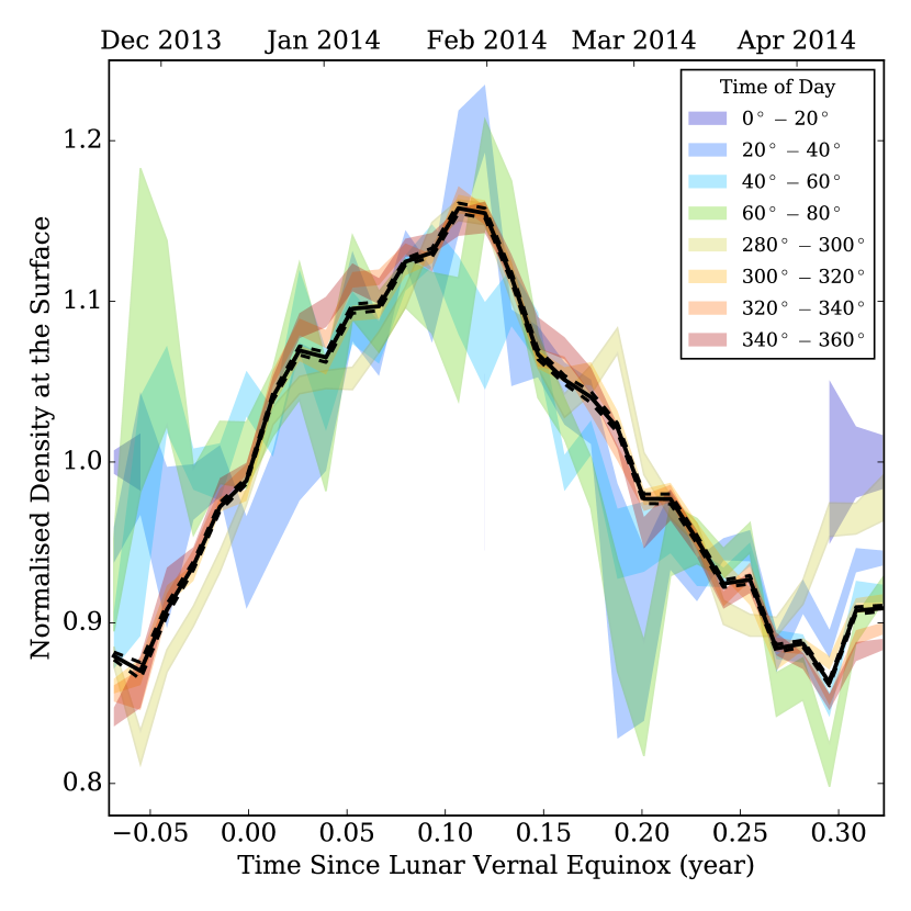
Figure 2: The long-term variation in the LADEE argon density, normalised by the mean density. The different colours show the median variation and its 1$\sigma$ uncertainty at the corresponding local time of day, as given in the legend. The solid black line shows the total mean variation, weighted by the errors on the time-of-day values. Dashed black lines represent the 1$\sigma$ uncertainty on this mean. Time is measured from the lunar vernal equinox on 17 December (Archinal et al., 2011).

As the argon abundance varies dramatically with the local time of day, to determine the long-term variation we first split the LADEE data into bins of 20^∘ in local time and calculate the mean density for each bin. The long-term variation is then calculated by subtracting the corresponding mean value from every measurement. To combine the data across all local times, we then divide by the same mean value to give the normalised deviation at a given long-term time. The median deviations are shown in Fig. 2, along with the weighted mean of all of these curves. The general agreement across the different times of day is notable, as is the relatively smooth variation.

The peak-to-peak change in density is 28%. Benna et al. (2015) noted the somewhat similar magnitude and timescale of the variation to that observed by LACE, and offered that transient changes in the release rate of argon from the Moon’s interior are a plausible cause of this variability. Hodges and Mahaffy (2016) instead suggested that it is part of a periodic fluctuation with a period of half a year. They proposed that this is driven by seasonal variations in the polar cold trap areas.

All subsequent figures in this section show densities at the surface with the mean long-term variation removed from the data. This is done by dividing each data point by the normalised long-term variation at the time of the measurement. This reveals what LADEE would have observed had the exosphere been in a steady state.

2.3 Local Time of Day

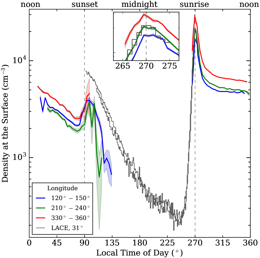
Figure 3: The variation of the argon density with local time of day. The coloured lines are typical examples of the LADEE data across the mare (red) and highland (blue and green) selenographic longitude regions, as given in the legend. The shaded areas represent the $\pm 1\sigma$ uncertainties. The inset plot zooms in on the region around the sunrise peak. The grey lines are two sets of LACE data separated by a few lunar days (Hodges, 1975) and normalised to match the density from LADEE at LACE’s location at sunrise. A vertical slice would yield the distribution of density with longitude at that time of day, as shown in Fig. 4.

Fig. 3 shows the distribution of argon with local time of day from LADEE and LACE data, with the LADEE data corrected for altitude and long-term variability as described above. The figure shows just three representative examples across the mare and highland regions for clarity. The LADEE (and LACE) data show very similar behaviour at all selenographic longitudes. In particular, the timing of the sunrise peak is insensitive to the longitude, as highlighted by the inset panel, occurring at local times between ${269^{\circ}\pm 1^{\circ}}$ and ${272^{\circ}\pm 1^{\circ}}$. However, the argon density is greater in the maria than that in the highlands by a factor that ranges from a few tens of per cent up to almost a factor of 2 at sunrise. The LACE densities have been rescaled in amplitude to match the inferred surface density at sunrise from LADEE at the location of LACE, to extract the long-term variation between the data set. Note that the lowest late-night LACE measurements may be below the instrument’s sensitivity (Hoffman et al., 1973).

The large peaks in density around sunset and sunrise are both fed by particles migrating away from noon, where the higher temperatures mean larger hops. At sunset, the temperature is lower, so particles do not hop very far, but it is not yet cold enough to trap argon on the surface for long periods of time. Any particles that do stick to the surface at night will rotate with the Moon toward sunrise, creating the enormous peak when they warm up at dawn and reenter the exosphere. This peak extends back into the night because the particles fly in all directions, with a typical hop distance of a few degrees at post-sunrise temperatures.

2.4 Selenographic Longitude – The Bulge

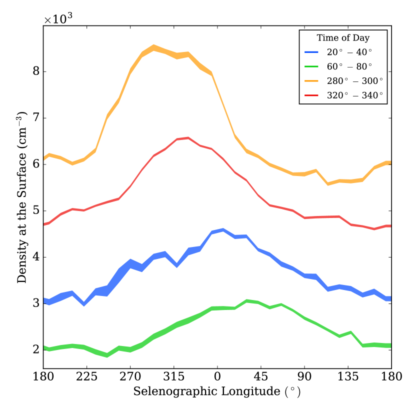
Figure 4: The variation of argon density with selenographic longitude from LADEE, showing the bulge over the western maria and its evolution through the lunar day. The coloured regions show a selection of different local times of day, the shaded areas represent the $\pm 1\sigma$ uncertainties. A vertical slice would yield the distribution of density with time of day at that longitude, as shown in Fig. 3.

The change of density with selenographic longitude is shown in Fig. 4 for different slices in local time of day. As was evident from Fig. 3, the density at all local times of day is highest at some point over the maria (longitudes from 270^∘–$45^{\circ}$). The peak near sunrise is located over the western maria in the region of the Procellarum KREEP Terrain (PKT), which is rich in ⁴⁰Ar’s parent, ⁴⁰K (Jolliff et al., 2000). Along the different curves of fixed local time, the selenographic longitude of the peak argon density drifts systematically from $\sim$300^∘ at sunrise to $\sim$45^∘ at sunset.

These distributions all reflect a complex interplay between sources, sinks and, most importantly, surface interactions of the argon atoms. Consequently, the variation of argon density with both selenographic longitude and local time of day offer the opportunity to distinguish between different models for the argon exosphere.

3 Model

In this section, we describe the main processes and input parameters in our model. Appx. A contains full details of aspects of our model that differ from similar previous studies such as that by Butler (1997). The simulation code itself is publicly available with documentation at icc.dur.ac.uk/index.php?content=Research/Topics/O13.

The central idea is to follow one particle at a time throughout its life, then repeat this for many particles to build up a model of the lunar argon exosphere. Each simulation particle represents a number of argon atoms, and in between its creation and eventual loss from the system, it migrates in a series of interactions with the surface and ballistic hops. The models for each of these various processes are now described in turn.

3.1 Source

Most of our simulations are for a steady-state exosphere in which the continuous source rate matches the loss rate, after an initialisation period in which more particles are created than are lost. We assume a continuous source given the relatively smooth variation observed by LADEE, which suggests a lack of dramatic transient source events. The source rate, the mean lifetime, and the total number of particles in the equilibrium system are directly related – knowing any two determines the third. In our simulations, we can investigate a range of mean lifetimes by varying the sinks. The total amount of argon in the exosphere is then scaled to match that from the LADEE measurements by setting the source rate.

The value for the source rate is implicitly varied in a range that reflects the uncertainty in the amount of potassium in the Moon and the effectiveness with which radiogenic ⁴⁰Ar reaches the surface. Killen (2002) modelled argon’s production and diffusion from the potassium in the crust and estimated that argon enters the exosphere at a rate in the range of 3.8–5.5$\times 10^{20}$ atoms s^-1. These values correspond to only a few per cent of the ⁴⁰Ar that is created inside the Moon (Hodges, 1975), so we also investigate significantly higher source rates.

Following the discussion from Benna et al. (2015), we wish to test if a (continuous) localised source can reproduce the argon bulge over the western maria and, if so, what source and loss rates this would require. Thus, we use either a global source, where the argon particles appear isotropically at random locations on the spherical surface, or a local source, where they appear preferentially at locations with higher near-surface potassium concentrations. As noted by Benna et al. (2015), while argon is expected to originate from deep, molten sources, there may be preferred diffusion pathways up through the same region marked by the potassium and PKT. The LPGRS, and more recently gamma-ray spectrometers on board Chang’E-1 and Chang’E-2, measured the potassium abundance and distribution in the top metre or so of the regolith (Prettyman et al., 2006; Zhu et al., 2011, 2015). For the localised source model, we use the LPGRS potassium map to weight the source distribution for the simulation particles, such that the probability of being sourced at a given location is proportional to the local potassium concentration.

3.2 Sinks

There are two main ways in which particles can be lost from our simulations: interactions with photons or charged particles from the Sun; and cold trapping on the surface in the permanently shadowed polar regions. Our implementation of these physical processes is described in the following subsections. We include the possibility of gravitational escape in our simulations, but for argon this has a negligible effect.

3.2.1 Solar Radiation

A particle in flight on the dayside may be lost due to a variety of processes, the most important of which are photoionisation and charge-exchange with solar wind protons (Grava et al., 2015). An ionised particle will rapidly be driven either away from or into the Moon’s surface by the local electromagnetic field. Those that impact the surface may be neutralised and “recycled” back into the exosphere. Following Butler (1997) and Grava et al. (2015), such processes can be combined to give a single solar radiation destruction timescale, $\tau$. The probability of loss during a flight of time $t$ is then

$$P(t)=1-e^{-t/\tau}\;.$$ (2)

For each particle hop, our algorithm picks a random number from a uniform distribution between 0 and 1. If this lies below $P(t)$, then the particle is removed from the simulation.

During LADEE’s operation, the mean solar wind speed and proton density were 400 km s^-1 and 5 cm^-3 respectively (from the GSFC/SPDF OMNIWeb database interface at omni-web.gsfc.nasa.gov), giving a proton flux of $2\times 10^{8}$ cm^-2 s^-1. Multiplying this by the interaction cross section, $2\times 10^{-15}$ cm² (Nakai et al., 1987), gives a rate for proton-argon charge-exchange of $4\times 10^{-7}$ s^-1. Adding the photoionisation rate from Huebner et al. (1992), $3\times 10^{-7}$ s^-1, taking the inverse, and finally dividing by the recycling fraction of 0.5 (Poppe et al., 2013), gives a timescale of $\tau=3\times 10^{6}$ s. Including the recycling process by simply increasing the timescale is analogous to assuming that a recycled ion reenters the exosphere without travelling a long time or distance. Many of these values have significant uncertainties, such as the cross section which has a somewhat broad peak around 1 keV protons, and the solar wind speed and proton density, which fluctuate significantly. Thus, this error on this timescale is likely at least a factor of 2.

3.2.2 Cold Traps

If a particle lands in a permanent cold trap near the poles, then it is assumed to stick there indefinitely. Like previous models, we adopt a stochastic approach. When a particle lands within $15^{\circ}$ of the north or south pole, it has a probability of being trapped, given by the total fractional area of cold traps in that polar region. Various estimates have been made for the size and distribution of cold traps. The appropriate cold trap area depends on the surface interaction of the specific species and the complicated processes that may occur after landing in a cold trap, either to secure or remove the particles (Schorghofer and Aharonson, 2014; Chaufray et al., 2009). As the uncertainty on the effective cold trap area is large, we leave this as a free parameter.

Fig. 5 shows the mean lifetime (and corresponding source rate) of argon atoms in the exospheric system for different cold trap areas, keeping the photodestruction timescale constant and using the surface interaction models described in the following subsection. Larger cold traps result in shorter lifetimes, and a larger source rate is then required to maintain the same total number of argon atoms. Also shown in Fig. 5, for reference, are some maximum surface temperatures and their corresponding cold trap areas, as inferred from Diviner data (Vasavada et al., 2012). This is done by relating a given cold trap area to the same-size area that never exceeds a certain temperature.

For our default surface interaction model, the total argon content in the simulation is set at ${4\times 10^{28}}$ atoms to match the LADEE abundance measurements. The main uncertainty in this number arises from the long-term and selenographic variations in density measured by LADEE, amounting to about 44%.

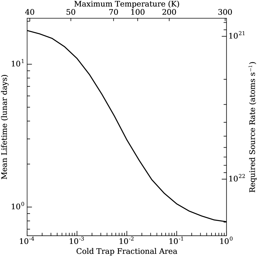
Figure 5: The mean lifetime of the simulated argon particles for different cold trap areas as fractions of the polar 15^∘. The right axis shows the source rate of argon that would be required to match the inferred LADEE total argon abundance. The top axis gives the maximum surface temperatures from Diviner that correspond to the assumed areas covered by cold traps.

3.2.3 Seasonal Cold Traps

We include the possibility of seasonal cold traps in our model in addition to the permanent cold traps. These have fractional areas in the north and south polar 15^∘ that grow and shrink periodically as

$$\begin{split}f_{\text{N}}&={\rm max}\left[0\,,\,f_{\text{peak}}\sin\left(2\pi\,(t_{\text{yr}}-0.5)\right)\right]\\ f_{\text{S}}&={\rm max}\left[0\,,\,f_{\text{peak}}\sin\left(2\pi\,t_{\text{yr}}\right)\right]\;,\end{split}$$ (3)

where $f_{\text{peak}}$ is the peak fractional area and $t_{\text{yr}}$ is the time in units of years. Thus, the year begins with the vernal equinox and the southern trap reaches its maximum size one quarter of the way through the year, followed by the autumnal equinox and the northern peak in turn. The seasonal traps disappear completely in the summer half of the year for that pole. This asymmetry is required to match the half-year period suggested by the data (see Fig. 2). If instead the seasonal traps varied symmetrically in both halves of the year, for example, sinusoidally as in Eqn. 3 but without truncation, then the summed seasonal trap area of both poles would vary with a period of 1 year – or be constant if the maximum area at each pole were the same. Thus, a model must have the same overall half-year period to have the potential to explain the data. This requires asymmetrical variation in summer and winter, as is modelled simply by Eqn. 3.

At the time a particle lands in a seasonal trap, there is a distribution of times at which the present cold traps first appeared (and hence the times at which they will disappear), following Eqn. 3. Some will have appeared at the beginning of that pole’s winter and others potentially just before the particle landed. A particle that lands in a seasonal cold trap is released back into the exosphere at a randomly chosen time, following this distribution.

3.3 Hop Trajectory

In the absence of forces other than the gravity from the Moon, the complete paths of particles – including the landing position, time of flight, and position and velocity at any altitude – can be calculated analytically from the starting location and velocity using Kepler’s laws (see Appx. A.2). This approach is much less computationally intensive than integrating the paths numerically, even when positions and velocities are also calculated at altitude. This is how we transport particles in our simulation and, apart from the time of flight, it matches the approach of Butler (1997) and Crider and Vondrak (2000) for finding the landing position. For their time of flight calculation, they effectively assumed that the surface is flat, leading to slightly underestimated flight times.

For the initial velocity, the particles are assumed to have accommodated to the surface temperature at their starting location and to have a Maxwell-Boltzmann distribution in the exosphere for that temperature. This means that the initial speed for a particle leaving the surface must be drawn from the Maxwell-Boltzmann flux distribution (Brinkmann, 1970; Smith et al., 1978). As each particle represents a small packet of argon atoms moving through the surface, the random emission direction in the outward hemisphere needs to be weighted by the component of the speed in the vertical direction. The good fit of the simulation densities at altitude to the LADEE data suggests that this model is appropriate. Another difference between our treatment and those of Butler (1997) and Crider and Vondrak (2000) is that they chose emission angles away from vertical, $\alpha$, from a non-isotropic distribution that was uniform between 0 and $\pi/2$, without including the $\sin(\alpha)$ term that accounts for the full area of the emission hemisphere.

3.4 Surface Interaction

The interaction of argon with the surface determines many of the exosphere’s characteristics. However, it is a complicated and poorly understood process. In our model, once a particle lands it is assumed to adsorb immediately. It will then reside upon the surface for some amount of time before being released. The residence time and the kinematics of the desorbed particle both depend sensitively upon the temperature at the location of the particle. During the lunar night, the simulated particle may also “squirrel” down into the regolith, to resurface at some time the following day. This process turns out to be required to match the observed density distribution with local time of day while maintaining realistic desorption energy values, as is discussed in section 4.1.

The Diviner radiometer on the Lunar Reconnaissance Orbiter (LRO) produced temperature maps of the lunar surface (Vasavada et al., 2012). We use the analytical fit to the Diviner data from Hurley et al. (2015) to make a map of temperature as a function of local time and location in square-degree bins. Following Hurley et al. (2015), we also introduce a longitudinal Gaussian scatter with ${\sigma=4.5^{\circ}}$ into this map to account, statistically, for topographical relief. This represents the temperature effects of, for example, the orientation of slopes near sunrise, which will receive sunlight at different incidence angles, or the positions of ridges or craters that could see sunrise earlier or later respectively.

3.4.1 Residence Time and Desorption

Every ${\Delta t=5}$ s (a time step is only introduced in this part of the simulation), the temperature is re-calculated for a particle residing on the surface, to account for the Moon’s rotation. This allows a residence time, $t_{\text{res}}$, to be found using a standard modified Arrhenius equation (Bernatowicz and Podosek, 1991):

$$t_{\text{res}}=\dfrac{h}{kT}\exp\left[\dfrac{Q}{RT}\right]\;,$$ (4)

where $h$ is Planck’s constant, $R$ is the gas constant, $T$ is the temperature, and $Q$ is the desorption energy.

The probability of the particle desorbing from the surface in a given time step is

$$P(t_{\text{res}})=e^{-\Delta t/t_{\text{res}}}\;.$$ (5)

If a uniform random number between 0 and 1 exceeds $P$, then the particle is released and hops again. Otherwise, the simulation time is advanced by $\Delta t$ and the particle’s position and the local temperature are updated. This continues until the particle is released.

For argon, a barrier-free adsorption process is expected, so heats of adsorption and activation energies for desorption can be equated, both corresponding to $Q$. Experiments with argon on non-lunar aluminosilicates and mineral oxides have shown that the desorption energy is typically around 8–10 kJ mol^-1 (Matsuhashi et al., 2001). This increases slightly for more Lewis acidic materials, although higher values were obtained for the heat of adsorption, up to 24 kJ mol^-1 for some acidified mineral oxides, possibly being representative of lower coverages or corresponding to a small fraction of more strongly adsorbing sites. The surface composition of the Moon is dominated by anorthosite, comprised primarily of a variety of silicate minerals (Cheek et al., 2013; Wieczorek et al., 2006). Therefore, these terrestrial experiments provide a reasonable basis for estimating plausible values of $Q$.

On a low-energy metal oxide surface facet, Dohnálek et al. (2002) calculated the coverage-dependent desorption energy for argon from temperature-programmed desorption (TPD) data and found it to increase from 8 kJ mol^-1 to around 13 kJ mol^-1 at very low coverages (where only the highest energy sites should be occupied by argon atoms). If surface diffusion occurs readily and the coverage is low, then these strong adsorption sites may be accessible to all adsorbing argon atoms. Direct calorimetric heats of adsorption on another porous silica yielded $Q$ values of 18 kJ mol^-1 (again at low surface coverages of argon, Dunne et al., 1996). Interactions with the pristine lunar regolith may be even stronger (Farrell et al., 2015), and Bernatowicz and Podosek (1991) found with a freshly crushed lunar sample that somewhat-higher energies of up to 31 kJ mol^-1 (7.4 kcal mol^-1) are plausible. We conclude that experiments show we should expect argon-regolith interactions to involve energies around 10-30 kJ mol^-1. However, until more in-situ experiments are performed, the precise value must be estimated empirically using observations of the exosphere as a whole.

3.4.2 Squirrelling

Argon particles enter the exosphere by migrating up through the porous regolith from the Moon’s interior (Killen, 2002). We propose that some proportion of the particles residing on the surface will migrate randomly downward as well, to reenter the exosphere at a later time. A somewhat similar process has been discussed in Hodges (1982) and modelled for water ice in polar cold traps by Schorghofer and Aharonson (2014). As is discussed in section 4.1, we find that such a process is required to explain the LADEE data while maintaining realistic desorption energies.

The persistent reservoir of adsorbed particles residing on the surface at night would therefore act as a source for building up a distribution of particles with depth by the end of the night, which then re-emerge during the day. Section A.4 shows that these timescales arise naturally from the regolith structure and temperature. We assume that particles on the dayside do not adsorb frequently enough for long enough to “squirrel” in significant numbers.

We use a very simple model to investigate the effect this process has on the exosphere. Any particle adsorbed to the nighttime surface is given a small (constant) probability, $P_{\text{sq}}$, of becoming buried in the regolith. If this happens, then the particle will reenter the exosphere at some time during the following day. That is, the simulation time for the particle is advanced until the Moon has rotated it into a random local time on the dayside, with a uniform probability distribution. The particle “emerges” residing on the surface, then will desorb and hop as normal.

It is likely that this process is much more complicated in reality, with a dependence on temperature, gradients of temperature and density, and other factors. As one such example, just after sunrise, the subsurface is colder than the surface. This temperature gradient would discourage particles from migrating upward, perhaps delaying the resurfacing of some squirrelled particles until later in the day than would otherwise be expected. Given these uncertain issues, we note the necessary simplicity of this model and use it to explore the plausible effects of the process.

The uncertain surface interaction parameters $Q$ and $P_{\text{sq}}$ are varied in the next section, to determine the best values to describe the LADEE and LACE results.

4 Results and Discussion

In this section, we compare our simulations with the data introduced in section 2. First we show how the treatment of surface interactions affects the variation of argon with local time of day. Then we investigate the competing hypotheses to explain the argon bulge over the western maria. In the final part of this section, we study the possibility of seasonal cold traps being the cause of the long-term variation in the LADEE argon abundance.

4.1 Distribution with Local Time of Day

The sensitivity of the simulated exosphere to the values of the model parameters describing the surface interactions is shown in Fig. 6. In the left panel, the desorption energy, $Q$, is varied by $\sim$20% with the squirrelling process switched off, whereas the right panel shows how the distribution changes when the squirrelling probability, $P_{\text{sq}}$, is altered with fixed ${Q=28}$ kJ mol^-1.

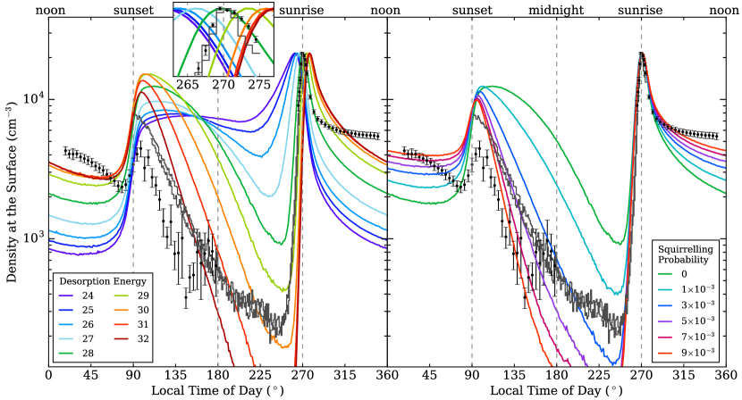
Figure 6: The variation of the argon density as a function of local time of day. (left) The desorption energy is varied and no squirrelling is included. The labels show the model desorption energy, $Q$, in kJ mol^-1 and the inset plot zooms in on the region around the sunrise peak. (right) ${Q=28}$ kJ mol^-1 and the model squirrelling probability is varied as shown in the legend. In both Figures 6 (left) and 6 (right), the distributions are normalised to match the peak data density to aid comparison of the shape. The mean data and 1$\sigma$ errors from LADEE across all longitudes are shown with black points and the LACE data are shown with grey lines.

While the higher desorption energy curves best match the nighttime rate of decrease of argon observed by both LACE and LADEE, these model surfaces are so sticky that the timing of the sunrise peak is delayed too far into the day to match the measurements, as highlighted by the inset panel. The sunrise peak position is sensitively dependent upon the model desorption energy. Given that the sunrise peaks are at the same local time over the highlands and maria (section 2.3), this suggests that the argon interactions with the surface are similar in these different regions.

Fixing the desorption energy at ${Q=28}$ kJ mol^-1 in order to match the sunrise peak position, the model predicts too much exospheric argon late in the night and too little during the day. This provides empirical motivation for the inclusion of the squirrelling process, which allows argon atoms to build up a subsurface population in the regolith overnight that is released throughout the following day. Increasing $P_{\text{sq}}$ enables us to produce a model that matches the nighttime decrease in argon and the shape of the sunrise peak, as shown in Fig. 6 (right). For our fiducial value of ${P_{\text{sq}}=5\times 10^{-3}}$, the simulation agrees within a factor of 2 with the observations over the entire lunar day. The behaviour from mid-morning to sunset is somewhat discrepant, but given the simplicity of our model and the fact that these details do not change any of the subsequent results and conclusions, we do not complicate the model further.

In contrast to our squirrelling approach, Hodges and Mahaffy (2016) adopted a bespoke temperature-dependent desorption energy (up to $\sim$120 kJ mol^-1 at noon) to bring their model into agreement with the LADEE measurements. Introducing all of this freedom into the model can lead to a good fit, but, as Hodges and Mahaffy (2016) themselves noted, such high desorption energies do “not comport with thermal energies”. The energies required by their model during the day are far beyond the bond strengths that argon has been measured to make or could be expected to make for the simple van der Waals interactions of a noble gas, as discussed in section 3.4. Any variable-energy model cannot affect the dayside densities significantly without resorting to these extreme values, because the high dayside temperatures make the residence times negligible for any lower desorption energies. Thus, the nighttime and sunrise densities cannot be simultaneously matched without either including a squirrelling-like process or using unrealistically high, temperature-dependent desorption energies. Note that we also tested a similar model for use in the following bulge and long-term investigations, and the subsequent conclusions were unchanged.

While our squirrelling approach provides a mechanism for fitting the nighttime and daytime argon abundances using physically plausible desorption energies, the simplifications that this model entails should be noted. These processes have not been extensively studied with argon on terrestrial materials, let alone in situ (Dohnálek et al., 2002). In reality, there will be a range of adsorption sites with somewhat different desorption energies, and the probability of adsorption will vary depending upon both the speed of the incoming atom and the presence of volatiles already on the surface. For instance, experiments show that argon has about a 70% probability of adsorbing to a surface at typical exospheric impact speeds of 300 ms^-1 but much lower temperatures of 22 K (Dohnálek et al., 2002). This probability decreases rapidly with higher impact speeds, reaching zero for 550 ms^-1. Argon is also more likely to stick when other argon atoms are already residing on the surface (Head-Gordon et al., 1991). The 300 ms^-1 adsorption probability reaches one when the coverage is roughly a monolayer. These values may of course be somewhat different for adsorption to the lunar regolith. Note also that the value of $Q$ depends on the exact form of Eqn. 4. So, it should not be interpreted as a precise estimate of the true energy, especially given the aforementioned details that are all approximated into this single parameter. For example, Grava et al. (2015) used a different prefactor and an extra free parameter, so their fitted value of $Q=27$ kJ mol^-1 results in a curve with the sunrise peak around 275^∘, comparable to our $Q=30$ kJ mol^-1. We focussed on fitting the observed sunrise peak time at 270^∘, so find an effectively lower energy.

We ran additional simulations to investigate the sensitivity of our results to these adsorption issues. Lowering the adsorption probability has a similar effect to lowering the desorption energy. Even for an adsorption probability below 0.1, an increase of a few kJ mol^-1 to $Q$ results in a similar distribution and sunrise peak position. A speed-dependent adsorption probability also does not dramatically change the distribution, compared with the effects from changing $Q$ or $P_{\text{sq}}$. More importantly, no such mechanisms appear to reduce the need for the squirrelling process to match the high dayside densities. So, while these known simplifications affect the results at a level that could explain some of the small discrepancies between the model and data distributions, our main conclusions are not sensitive to these assumptions.

One final consideration is the cold trap area and corresponding source rate. The above simulations were all run with the low permanent cold trap fractional area of 0.01% (of the polar 15^∘) that approximately corresponds to the low source rates estimated by Killen (2002). The much larger traps and high rates considered in the next section have the effect of increasing the density toward the end of the night, which improves the match to the minimum LACE densities (although these may be below LACE’s sensitivity (Hoffman et al., 1973)), due to the emergence of newly created particles through the night. The distribution is unaffected at other local times of day.

4.2 Longitudinal Bulge

There are two alternative hypotheses for the origin of the argon bulge over the western maria: (1) it reflects a spatially variable source rate that is higher over the western maria (Benna et al., 2015); or (2) it reflects a lower desorption energy from the western maria (Hodges and Mahaffy, 2016). We perform simulations using either a localised source reflecting the LPGRS potassium map (and our ${Q=28}$ kJ mol^-1, ${P_{\text{sq}}=5\times 10^{-3}}$ model described in section 4.1), or a uniform global source and a spatially varying desorption energy to examine these two scenarios.

For the case of a local source with a greater release of argon over the western maria, the amplitude of the bulge depends sensitively on (1) how localised the source is and (2) the source rate, or – equivalently in the steady state – the loss rate. For a diffuse source, a rapid turnover of particles with short lifetimes is necessary to produce argon atoms that have not travelled so many times around the Moon that their locations no longer reflect their origin. We ran simulations with a local source (proportional to the LPGRS potassium abundance) with a range of cold trap fractional areas to determine the area required to produce a bulge comparable with that observed by LADEE.

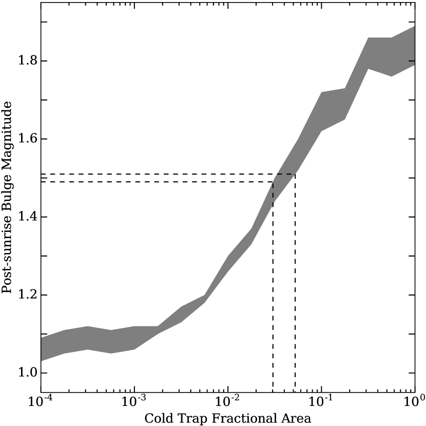
Figure 7: The magnitude (the ratio of the maximum to minimum densities over all longitudes at a given time of day) of the simulated bulge over the western maria (in this case at 280^∘–$300^{\circ}$ local time of day), generated by the localised source, for different values of the cold trap fractional area of the polar 15^∘. The dashed lines show the magnitude and uncertainty of the bulge measured by LADEE at the same local time and the corresponding range of cold trap areas.

Fig. 7 shows the amplitude of the post-sunrise (280^∘–$300^{\circ}$) argon bulge over the western maria. As shown by the dashed lines, to match the LADEE maximum-to-minimum ratio of ${1.5\pm 0.1}$, a cold trap fractional area of ${4\pm 1}$% of each polar 15^∘ is necessary, corresponding to a mean lifetime of $\sim$1.4 lunar days. This area is comparable with the $2$–$2.5$% covered by PSRs (Mazarico et al., 2011), but is uncomfortably large if argon is only supposed to be permanently trapped in regions with temperatures never exceeding $\sim$40 K (Hodges, 1980b). As indicated in Fig. 5, cold traps of this large size appear to correspond to regions with temperatures that can reach as high as 175 K.

Therefore, for this to be a viable model, one would either need argon to be more readily lost from the exospheric system than previously anticipated, or to have a more highly localised source below the surface than the LPGRS near-surface potassium map. To further investigate the degeneracy between the source rate and how localised the source is, we also tested a “top-hat” and a point source in the same way. The top-hat source emits argon uniformly from all regions with at least 2,000 ppm of potassium, giving a source region covering 6% of the Moon’s surface area in the PKT. This can create an argon bulge with the required amplitude with a cold trap fractional area of only 0.4%, a lifetime of 5.3 lunar days, and a source and loss rate of ${2.9\times 10^{21}}$ atoms s^-1. For the extreme case of a point source at 335^∘ longitude on the equator, a cold trap fractional area of 0.2% is sufficient, with a lifetime of 8.1 lunar days and a rate of ${1.9\times 10^{21}}$ atoms s^-1.

If the source is not quite so localised, then feasible causes of increased losses might be: an abundance of small-scale cold traps such as those inferred on Mercury (Paige et al., 2014; McGovern et al., 2013); the presence of other volatiles in PSRs increasing the adsorption probability (Dohnálek et al., 2002); and an unaccounted-for loss mechanism that means that our assumed solar radiation loss rate is an underestimate (recall the large uncertainty on this value as mentioned in section 3.2). Thus, this model begs an explanation either for the high source and loss rates, or for a highly localised source. Noting this tension, we press on to investigate the shape of the argon bulge in the simulation from the localised (potassium-weighted) source with a cold trap fractional polar area of 4% and compare it with the data.

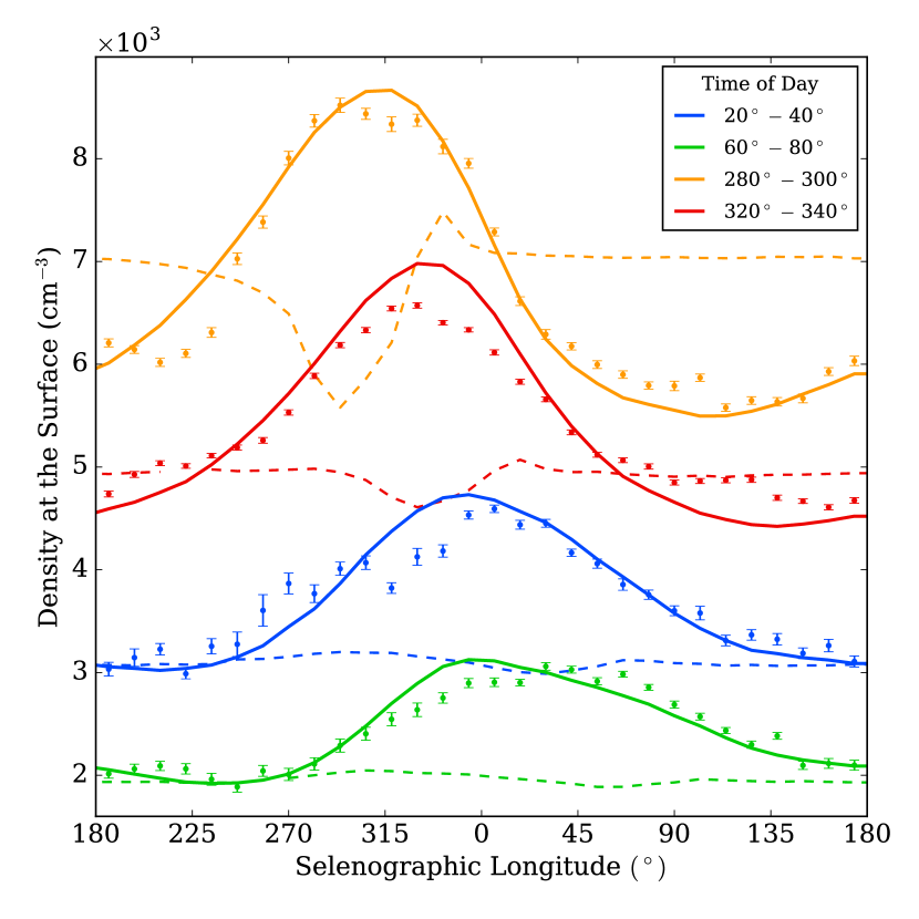
Figure 8: The variation of argon density with selenographic longitude for a representative selection of local times of day, shown by the different colours as defined in the legend. The solid lines show the bulge from the local source model with high rates of source and loss, the LADEE data are shown as points, and the dashed lines show the results for the global source with a lower desorption energy in the mare region than in the highlands (26 and 28 kJ mol^-1 respectively).

The variation of argon density with longitude in our simulations is shown in Fig. 8 for a sample of different local times of day. The solid lines result from the local source and large cold traps. The dashed lines are from the alternative hypothesis of an isotropic source with mare and highland desorption energies of ${Q=26}$ kJ mol^-1 and 28 kJ mol^-1 respectively, with a low cold trap fractional area of 0.01% (of the polar 15^∘) that corresponds approximately to the source rate estimated by Killen (2002). (Note that with an isotropic source the shape of the bulge is insensitive to the source rate.) Also reproduced are the LADEE results. We are predominantly interested in the shapes of the different curves, and not their relative amplitudes, which are determined by the local time of day distribution and are slightly different at certain times, as discussed in section 4.1. Thus, for clarity, each model curve was divided by its mean and multiplied by the mean of the corresponding data set.

The model with the local source was tuned only to match the maximum-to-minimum ratio of the post-sunrise argon bulge over the western maria observed by LADEE. However, the relative sizes of the bulge at all other times of day, the position, width, and shape of the bulge, and the shift of the bulge to the east throughout the day also happen to be reproduced well. These features result from the fact that the overnight build-up of argon over the western maria around longitudes $\sim$300^∘–$330^{\circ}$ diffuses rapidly across the sunlit surface after it reaches sunrise. This diffusion spreads out the peak in the argon density and shifts it into the dayside: that is, to the east. All these features are also reproduced with the top-hat and point sources, apart from the point source bulge being slightly narrower.

In contrast to the successes of this local source model, the effect of decreasing the adsorption energy over the western maria, shown by the dashed lines in Fig. 8, does not match any of the features in the data. The failure to reproduce the observations arises because the lower desorption energy encourages atoms to leave the surface and hop more frequently. This is successful in producing a bulge towards the end of the night, where the residence time is longest. However, it also rapidly evacuates the argon from the maria, and the nighttime bulge is replaced by a deficit in argon density almost immediately after sunrise. Therefore, trying to create a local overdensity in this way will inevitably fail if the bulge is required to persist throughout the day, as it is observed to do.

A separate reason to doubt this explanation is that these small changes in adsorption energy lead to significantly different local times for the sunrise peak in the mare and highland regions, in contrast to what the LADEE data show. Consequently, a spatially varying desorption energy explanation for the argon bulge can be ruled out for a couple of reasons. Similar arguments can be used to dismiss the idea that the bulge results from hotter surface temperatures for the maria, for example.

The local source is thus the only proposed hypothesis that has the potential to reproduce the variation of argon density with selenographic longitude seen in the data, and the results are remarkably similar. However, for this explanation to be successful, either (1) the lifetime of an argon atom in the exospheric system (i.e. from source to sink) needs to be $\sim$1.4 lunar days – if the source rate is proportional to the LPGRS potassium abundance; or (2) the source must be highly localised (or a slightly less extreme combination, as illustrated by the top-hat model). For the diffuse source, the required source rate of ${1.1\times 10^{22}}$ atoms s^-1 is about 46% of the total rate of argon produced in the Moon (Hodges, 1975), which is unlikely to be able to reach the surface unimpeded. The correspondingly high loss rate that this implies appears to demand widespread polar cold-trapping of argon that exceeds what had previously been considered. Assuming that the cold traps have been stable for $\sim$1 Gyr (Arnold, 1979), this means that the order of $10^{13}$ kg of argon would have been delivered to the polar regions during this time.

With this high cold trap fractional area of 4%, it takes roughly six lunar days from the start of the simulation before the exosphere reaches an equilibrium of source and loss rates and a stable number of argon atoms. In comparison, the time it takes for the equilibrium shape of the distributions to become established is always very short, on the order of one lunar day. This timescale is the same even with much smaller cold traps (such as those required for a highly localised source), for which the system can take a long time to reach a true steady state. This is analogous to saying that a localised event diffuses rapidly across the system, even if the total number of particles is still offset from equilibrium.

Irrespective of the lifetime and loss rate of argon in the simulation, particles spend 60% of their life residing on the surface, 30% squirrelling under the surface, and only 10% in flight in the exosphere. Thus, at any given time, these same proportions of the population of argon atoms will be residing on the surface, squirrelling, and in flight. The total number of argon atoms in the simulated exosphere at any time is about ${4\times 10^{28}}$, corresponding to a mass of 2,600 kg.

4.3 Long-Term Variation

Hodges and Mahaffy (2016) suggested that seasonally varying cold traps could produce a periodic signal responsible for the smooth long-term variation in the argon exospheric density by 28% over the 5 months of LADEE’s operation. As described in section 3.2.3, we have included seasonal cold traps to account for the fact that due to the 1.54^∘ obliquity of the Moon, when one pole is tilted away from the Sun, larger areas will act as cold traps for a few months. These seasonal traps would both temporarily remove and add argon, so they could drive changes in the density on the relevant timescale without a change in the overall source and loss rates. We performed simulations to test this hypothesis.

The magnitude of this variation is affected by the peak size of the seasonal traps and also by the source and loss rates, which in our model are controlled by the sizes of the permanent cold traps. For the low permanent cold trap fractional area of 0.01% (of the polar 15^∘) that corresponds approximately to the low source rate estimated by Killen (2002) (where solar wind losses dominate), the 28% change in the density seen by LADEE was reproduced with a peak seasonal cold trap fractional area of ${f_{\text{peak}}=0.8}$% at each pole’s midwinter.

The periodic long-term variation that is produced by these seasonal traps, at the latitudes probed by LADEE, is shown by the solid lines in Fig. 9, over a period of 1 year in the simulation. The peak density is predicted to be delayed by about 0.07 years (1 lunar day, $\sim$1 month) after the minimum trap size at the equinox. This is related to the time it takes for argon to travel between the poles and the equator and is remarkably similar to the delay in the LADEE data after the lunar vernal equinox, as shown in Fig. 9. Also shown is how much argon becomes trapped and released at each point in time throughout the year by the seasonal traps. Particles can be trapped from the beginning of winter until the very end, but are only released starting after midwinter, when the traps begin to shrink. This leads to a mild asymmetry in the long-term variation, which could easily be modified by deviating from our simple sinusoidal model.

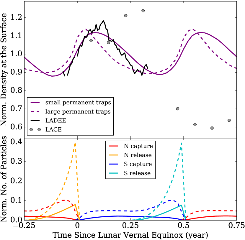
Figure 9: (top) The long-term variation of the argon population within 30^∘ latitude of the equator, normalised by the mean density. The purple solid line shows the normalised simulated density at the surface for the low rates model with permanent and peak seasonal cold trap fractional areas of 0.01% and 0.8% respectively; and the dashed line for a high rates simulation with areas of 4% (which reproduced the bulge for the localised potassium-weighted source) and 16%. Time is measured from the last lunar vernal equinox. The LADEE data are shown by the black line for comparison, and the grey points show the magnitudes of the LACE sunrise peak densities (Hodges, 1975) relative to the mean sunrise density measured by LADEE. (bottom) The number of argon particles that are being captured and released in each simulation by the northern and southern seasonal traps, given as a fraction of the total number of argon atoms in the equilibrium system (${4\times 10^{28}}$). The dashed lines show the results for the large permanent traps.

To demonstrate how the efficacy of the seasonal traps depends on the argon lifetime, we can attempt to reproduce the long-term variation with the very large permanent trap areas (4%) and higher loss rates that, with a localised source weighted by the near-surface potassium, would produce a bulge similar to the LADEE data. We found that much larger seasonal traps would be needed to cause the same magnitude long-term variation, with a peak fractional area of $f_{\text{peak}}=16$%. This is because, with much shorter particle lifetimes, fewer particles near the equator have been affected by the seasonal traps. In this case, a maximum of about ${2.6\times 10^{28}}$ argon atoms (over half of the steady-state exosphere) must be temporarily trapped to effect the 28% variation near the equator, over twice as much as in the low loss case. As shown by the dashed line in Fig. 9 (top), the delay of the peak density is also affected and occurs 0.04 years (one half lunar day) earlier. This timescale is sensitive to the evolution of the seasonal traps. It is possible that unaccounted-for factors such as thermal inertia, which could cause newly shadowed regions not to begin trapping immediately, delay the variation enough to reproduce the data even with high loss rates.

Unfortunately, the success of this seasonal model with the LADEE data does not continue for the long-term variation measured by LACE, which is shown by the grey points in Fig. 9 (assuming it is not the result of instrument degradation). The seasonal variation acts in the opposite way to the trend seen in 1973. Therefore, if there are seasonal cold traps that explain the LADEE argon data and they were active during the LACE measurements, then the loss rate required to match the drop measured by LACE needs to be significantly larger than had been anticipated by Grava et al. (2015). It is also noteworthy that the later LACE measurements fall well below the minimum measured by LADEE at the same location. This suggests that, if the LADEE data do show a periodic feature and there was not a transient loss event to drive down the later LACE measurements, then the equilibrium size of the exosphere must have increased over the last 40 years.

It is also possible that the LADEE and LACE long-term variations are both the result of transient source events, as suggested by Benna et al. (2015) and Grava et al. (2015). If we assume that the minima of the LADEE and LACE measurements indicate the equilibrium states throughout the measurement periods, and that a transient source had increased the density to the maximum before discontinuing, then we can model the decrease as a simple exponential decay from the maximum measurement back to the equilibrium state. In both the LADEE and LACE cases this would require a lifetime of around 0.9 lunar days, even shorter than that required for our local source bulge hypothesis and implying even greater loss rates. If the equilibrium level is lower than the minimum measurements, then the variations would therefore be part of even larger but less rapid declines. In the absolute limit of no background exosphere at all, the required lifetimes could extend up to nine and five lunar days for LADEE and LACE respectively. In this extreme case, these long lifetimes would require only small source and loss rates and correspondingly small permanent cold traps with temperatures below 70 K, as shown by Fig. 5. Similar arguments can be made regarding transient loss events, since LADEE shows an equally rapid increase of argon. Of course, it is imaginable that a combination of multiple, dramatic source and loss events could produce these variations regardless of the lifetime, but this is extraordinarily unlikely.

As discussed in section 3.2.3, asymmetrical variation of the seasonal traps in summer and winter is necessary to match the half-year period suggested by the data. Therefore, our model included no seasonal cold traps throughout the summer half of the year at each pole. Had we instead allowed some seasonal traps to decrease until the summer solstice, their reduction would have offset some of the effect of the growing traps at the other pole. Consequently, the model would have needed larger seasonal trap areas to match the amplitude of the observed long-term argon variation. It should be possible to use lunar elevation maps to predict the actual variation of seasonal cold traps throughout the year, at least enough to test whether such an asymmetrical variation is realistic. In the scope of this work, we show only that this hypothesis has the potential to explain the data.

5 Conclusions

We have studied the LADEE (and LACE) measurements of the lunar argon exosphere and developed a Monte Carlo model to investigate what is implied about the sources, sinks, and surface interactions in the system, and to test whether various hypotheses are able to explain the observed features.

The extrapolation of simulated density at an altitude of 60 km to density at the surface is fitted to within 12% everywhere using a model of two Chamberlain distributions with different temperatures. From this altitude, using a single Chamberlain distribution or its first order approximation can lead to overestimates greater than a factor of 3. These errors can be much larger for extrapolations from higher altitudes. Other exospheric species should exhibit similar behaviour. Lighter particles typically travel farther each hop, which would increase the error from using a single-temperature model. The two-temperature model fits the LADEE data well, suggesting that simple thermal desorption dominates the release energetics of exospheric argon.

The distribution with local time of day of the argon density in the exosphere is very sensitive to the nature of the interactions with the surface. Apart from an offset in amplitude reflecting the higher density over the maria, the highland and mare results are very similar, suggesting that the surface interactions do not differ greatly with regolith composition at equatorial latitudes. A very simple model allowing atoms to squirrel into the regolith overnight, building up a subsurface population that is released during the following day, can reproduce the broad characteristics of the observed exosphere at all times of day, without the need to resort to unreasonably high and temperature-dependent desorption energies. The timing of the sunrise peak requires a residence time near sunrise of 1,300 s, which corresponds to a desorption energy of 28 kJ mol^-1, a high but plausible value for noble gas interactions. The subsequent results are insensitive to the details of these surface interaction models.

Of the two hypotheses that have been proposed for the origin of the argon bulge over the western maria and PKT, only a localised source has the potential to explain this feature. Our simulations with this model can reproduce the observed size, shape, and position of the bulge at all local times of day. There is a degeneracy between how localised to the mare region the source is and the lifetime and rates that the data require. For a source distribution weighted by the LPGRS potassium map, the observed bulge is reproduced with a mean lifetime for argon atoms in the exospheric system of only 1.4 lunar days, corresponding to a high equilibrium source and loss rate of ${1.1\times 10^{22}}$ atoms s^-1. To achieve this, our model would need permanent cold traps that have a total area comparable with the PSRs measured at Diviner’s resolution, or some other additional loss mechanism. A more highly localised source can reduce the required rates and trap areas by an order of magnitude – a point source reproduces a bulge of the right amplitude with a source and loss rate of ${1.9\times 10^{21}}$ atoms s^-1. So, despite this model’s unique success in reproducing the data, it begs an explanation for some combination of source localisation and high source and loss rates.

Models that aim to create the argon bulge by encouraging atoms to hop either more frequently or higher founder because they naturally lead to a short-lived feature through the night that is replaced by a local deficit in the argon density after sunrise.

The long-term variation in the global argon density seen by LADEE can be elegantly explained by the periodic behaviour of seasonal cold traps. The details of how large they need to be depend upon the base source and loss rates. The time lag of the peak density in the data is reproduced naturally by the model for small cold traps and low rates. It is slightly offset for higher rates, which might be mitigated by effects such as thermal inertia. However, the long-term decrease seen by LACE in 1973, if real, requires some other significant source and/or loss process because the seasonal variation should act in the opposite way to the observed trend. The relatively smooth variation of the argon density observed over the lifetime of LADEE suggests that significant transient release or loss events are unlikely to be the cause. This includes the apparent lack of a significant effect from the periodic crossing of the Moon through the Earth’s magnetotail, which might have been expected to reduce the solar wind loss rate. Any transient source (or loss) explanation would also require high rates of source and loss for the system to return to equilibrium after the event within the measured lunar-day timescales, unless the equilibrium density is far lower than the minimum observed by LADEE.

Seasonal cold traps should be expected to impact other species in the exosphere in a similar way, depending on their threshold trapping temperature. If any non-radiogenic, condensible species (such as methane) (Hodges, 2016) were also found to follow the variation seen for argon, then this would be strong evidence in support of the seasonal hypothesis (and vice versa). This is because tidal or seismic changes that might affect the argon source rate would be irrelevant for species that do not come from inside the Moon. Further long-term observations of the argon density would also help determine whether the variation is actually periodic in the first place.

There are several experiments that could help determine what combination of source localisation and rate of source and loss is responsible for the bulge, given the lack of other possible explanations. To test the hypothesis of a diffuse localised source with very high source and loss rates, one could pursue: in-situ searches for argon trapped in PSRs, although there are various uncertainties regarding how much sequestered argon would be found and at what depth (Schorghofer and Taylor, 2007); or measurements of the exosphere towards the poles, where the effects that large cold traps would have on the distribution of argon with latitude would be detectable. On the other end of the degeneracy: if the source is highly localised, then the large differences in that rate should directly affect the late-night argon distributions in the mare and highland regions. This might need to be measured at or near the surface to detect the very low densities. Future investigations of this kind would help determine if this model is indeed the origin of the bulge, or if some entirely new explanation is required.

Appendix A Theory and Derivations

This appendix contains the derivation of the hop trajectory and time of flight equations. Also included are details of the “simulation-fit” altitude model described in section 2.1 and a short calculation concerning the squirrelling mechanism described in section 3.

A.1 Notation

(a) Ellipse and circumcircle notation.

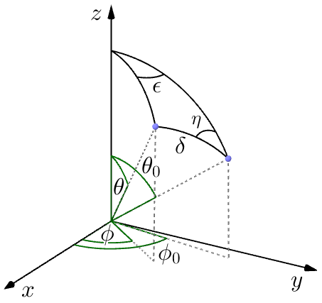
(b) Start and end point notation.

Figure 10: The notation for the dimensions, angles and areas: (a) $a,b,$ and $e$ are the semimajor axis, semiminor axis, and eccentricity of the ellipse, respectively. The variables $\theta$ and $E$ are the true anomaly and mean anomaly of the object at a distance $r$ from the focus; $\psi$ and $E^{\prime}$ are their complementary angles. The $\alpha$ and $v_{0}$ give the velocity of the object; $\alpha^{\prime}$ is the complementary angle. $A_{\psi}$ is the area of the outlined triangle $+$ ellipse section; $A_{1},A_{2},A_{3}$, and $A_{4}$ are the areas of the same-colour-shaded sections. The Moon is shown by the dashed circle; the blue points mark the start and end of a particle’s hop. (b) The subscript 0 denotes the initial position. The $\eta$ is the direction west from north of the particle’s initial velocity. The $\epsilon$ is the difference in longitude and $\delta$ is the total angle between the start and end points.

Figs. 10a and b show all the relevant notation for a particle’s hop. We use standard polar coordinates $\theta$ and $\phi$, with colatitude $\theta=0$ at the north pole, and standard selenographic longitude $\phi=0$ at the sub-Earth point. The local time of day, $\phi^{\prime}$, is given by the longitude relative to the subsolar point (noon, where $\phi^{\prime}=0$). To account for libration, the longitude of the subsolar point, $\phi_{\text{ss}}$, is calculated from JPL HORIZONS ephemerides (Giorgini, 2015) (latitude variations are ignored). The time of day is then simply ${\phi^{\prime}=\phi-\phi_{\text{ss}}}$. If we had ignored libration, then errors of over 3^∘ would have been introduced for some local times of day.

A.2 Hop Trajectory

Starting from the initial position and velocity of a particle, we can calculate the landing position (or the position at any altitude) by first finding the parameters of the elliptical path, shown in Fig. 10a. The vis viva equation gives the semimajor axis, $a$, in terms of the speed, $v$:

$$v^{2}=GM\left(\dfrac{2}{r}-\dfrac{1}{a}\right)\hskip 10.00002pt\Rightarrow\hskip 10.00002pta=\left(\dfrac{2}{r}-\dfrac{v^{2}}{GM}\right)^{-1}\;,$$ (6)

and the ellipticity, $e$, is found from the velocity angle $\alpha^{\prime}$:

$$\sin(\alpha^{\prime}) =\dfrac{r\dot{\psi}}{v}=\sqrt{\dfrac{a^{2}(1-e^{2})}{2ar-r^{2}}}$$ (7)

$$\Rightarrow\hskip 20.00003pte =\sqrt{1-\left(\dfrac{2ar-r^{2}}{a^{2}}\right)\sin^{2}(\alpha^{\prime})}\;\;.$$ (8)

The equation for an elliptical path can then be rearranged to give the angle $\psi$ in terms of $a$ and $e$:

$$r(\psi) =\dfrac{a(1-e^{2})}{1-e\,\cos(\psi)}$$ (9)

$$\Rightarrow\hskip 20.00003pt\psi =\cos^{-1}\left[\dfrac{1}{e}\left(1-\dfrac{a(1-e^{2})}{r}\right)\right]\;.$$ (10)

In Fig. 10b the angles $\delta$ and $\epsilon$ can be calculated along with the landing coordinates $\theta$ and $\phi$. At the start of the hop (${\psi=\tfrac{1}{2}\delta}$), Eqn. (10) becomes

$$\delta=2\cos^{-1}\left[\dfrac{1}{e}\left(1-\dfrac{a(1-e^{2})}{R}\right)\right]\;,$$ (11)

where $R$ is the radius of the Moon.

The spherical cosine rule gives

$$\begin{split}\theta=\cos^{-1}&\left[\cos(\theta_{0})\cos(\delta)\;+\right.\\ &\,\left.\sin(\theta_{0})\sin(\delta)\cos(\eta)\right]\;.\end{split}$$ (12)

Using the cosine rule again, but with $\epsilon$ instead of $\eta$, gives

$$\epsilon=\cos^{-1}\left(\dfrac{\cos(\delta)-\cos(\theta)\cos(\theta_{0})}{\sin(\theta)\sin(\theta_{0})}\right)\;.$$ (13)

Then $\phi$ is simply given by

$$\phi=\begin{cases}\phi_{0}+\epsilon\hskip 20.00003pt\eta>\pi\\ \phi_{0}-\epsilon\hskip 20.00003pt\eta<\pi\end{cases}\!\!\!.$$ (14)

The total time of flight is ${t=2t_{\psi}}$, where $t_{\psi}$ is the time the particle spends tracing out the area $A_{\psi}$ in Fig. 10a with its radial vector. Using general properties of ellipses, it can be shown that ${A_{\psi}\equiv A_{1}+A_{3}=\tfrac{b}{a}(A_{2}+A_{4})}$, and therefore

$$A_{\psi}=\tfrac{1}{2}\,ab\,\left(E^{\prime}+e\,\sin(E^{\prime})\right)\;.$$ (15)

The total period of the orbit, $T$, is given by Kepler’s third law:

$$T=\sqrt{\dfrac{4\pi^{2}a^{3}}{GM}}\;.$$ (16)

Kepler’s second law states that equal areas are swept out by the radial vector in equal times, therefore,

$$\begin{split}t_{\psi}&=T\dfrac{A_{\psi}}{A_{\text{ellipse}}}=T\dfrac{\tfrac{1}{2}ab(E^{\prime}+e\,\sin(E^{\prime}))}{\pi ab}\\ &=\dfrac{T}{2\pi}(E^{\prime}+e\,\sin(E^{\prime}))\;.\end{split}$$ (17)

Finally, the eccentric anomaly, $E$, is related to the true anomaly, $\Theta$, by

$$E=2\tan^{-1}\left[\sqrt{\dfrac{1-e}{1+e}}\tan\left(\dfrac{\Theta}{2}\right)\right]\;.$$ (18)

${E^{\prime}=\pi-E}$, ${\Theta=\pi-\psi}$, and here ${\psi=\tfrac{1}{2}\delta}$. Therefore,

$$E^{\prime}=\pi-2\tan^{-1}\left[\sqrt{\dfrac{1-e}{1+e}}\tan\left(\dfrac{\pi-\tfrac{1}{2}\delta}{2}\right)\right]\;.$$ (19)

This, with Eqn. (17), gives the time of flight.

A.3 Altitude Model Fitting

The “simulation-fit” model described in section 2.1 is a sum of two Chamberlain distributions with three free parameters: the relative amplitude of the two distributions and their different temperatures. The total amplitude is also free but is simply set by the observed density at altitude.

In order to fit these parameters at all local times of day and latitudes, we first obtained the simulated density at equilibrium for a range of altitudes (from 0 to 140 km in 10 km steps). The best-fit parameters for each square degree bin were then determined by finding the minimum $\chi^{2}$ for the simulation data.

These best-fit parameters are publicly available at icc.dur.ac.uk/index.php?content=Research/Topics/O13. In our steady-state model, the argon density near the end of the lunar night is extremely low, especially at high latitudes and altitudes. The LADEE data in these same regions were discarded, as discussed in section 2, so this was irrelevant for our analysis of the dataset. Thus, the best-fit parameters in these lowest-density regions were not examined in detail and may suffer from the fewer observed particles and high scatter in the simulation results.

This model is dependent on the argon distribution with time of day in the simulation. We repeated the analysis with a non-physical isotropic distribution, to quantify the maximum possible error that from discrepancies between our model and the real distribution. This amounted to $\sim$7% near the end of the night and below 1% elsewhere (within $\pm 30^{\circ}$ latitudes).

A.4 Squirrelling

We can estimate the statistical effect this downwards migration could have on the exosphere’s distribution with simple, order-of-magnitude considerations. The regolith temperature just 2 cm below the surface never drops below 200 K, and by 10 cm only varies by 15 K either side of 255 K (Teodoro et al., 2015).

For particles randomly migrating in the regolith throughout the lunar night ($\sim{10^{6}}$ s), with typical steps of size ${\lambda\sim 1}$ $\mu$m (around and between grains of $\sim\mu$m-mm diameters) and residence times of ${t_{\text{res}}\sim 10^{-7}}$ s (for ${T=255}$ K and ${Q=28}$ kJ mol^-1; so negligible traversal times of $\sim$10^-9 s at thermal speeds), they will take ${N\sim 10^{13}}$ steps, random walking a distance of ${\lambda\sqrt{N}\sim 1}$ m. This implies that a significant number of particles could bury themselves down into the regolith during the night, with the dense source of particles residing on the surface. By symmetry (since the temperatures below the surface are similar at all times), they will take a similar amount of time (the order of half a lunar day) to migrate out of the regolith and reenter the exosphere. This suggests a population of particles that squirrel into the regolith during the night and typically reenter the exosphere during the day.