Descendant log Gromov-Witten invariants for toric varieties and tropical curves

Abstract.

Using degeneration techniques, we prove the correspondence of tropical curve counts and log Gromov-Witten invariants with general incidence and psi-class conditions in toric varieties for genus zero curves. For higher-genus situations, we prove the correspondence for the non-superabundant part of the invariant. We also relate the log invariants to the ordinary ones, in particular explaining the appearance of negative multiplicities in the descendant correspondence result of Mark Gross.

1. Introduction

In a pioneering work [Mi], Mikhalkin proved a correspondence of counts of algebraic curves in a toric surface with analogous counts of certain piecewise linear graphs called tropical curves. Around the same time, Siebert and Nishinou [NS] used very different groundbreaking techniques (toric degenerations and log geometry) to prove a genus $0$ correspondence theorem in any dimension. Building on this second approach, this article generalizes both these results in the following directions:

• to allow $\psi$-conditions on the curves (i.e. to consider descendant invariants) because such conditions are particularly useful in various applications,

• to generalize to all non-superabundant situations (no a priori genus or dimension restrictions),

• to allow incidence conditions in the toric boundary for applications to non-toric situations like non-toric blow-ups or Calabi-Yau degenerations,

• to allow arbitrary tropical cycles as incidence conditions, not just affine linear ones.

To clarify: genus zero situations are always non-superabundant, but superabundant curves may contribute when $g>0$, especially if we also have $\dim\geq 3$, and also for $\dim=2$ if $\psi$-classes are present (see Remark 2.6). Even in these cases though, our result still gives the correspondence for the non-superabundant part of the invariant (in analogy to residual intersection theory).

Mikhalkin suggested in [Mi2, §3] that $\psi$-class conditions manifest in tropical geometry as higher-valence conditions at markings. Markwig-Rau [MR] and M. Gross [GrP2] proved genus $0$ descendant correspondence theorems involving higher-valent vertices for ordinary GW invariants of $\mathbb{P}^{2}$, later generalized by P. Overholser [Over] also for $\mathbb{P}^{2}$. Note also [Rau]’s work for $\mathbb{P}^{1}$ and $\mathbb{P}^{1}\times\mathbb{P}^{1}$. Notably, all these correspondence results are for ordinary Gromov-Witten invariants. We discuss the difference between these and the log invariants below.

Concerning genus $0$ log invariants, while our paper was in progress, [Ran] used ideas from tropical intersection theory to give a new proof of the Nishinou-Siebert result, and then A. Gross [AGr] extended these methods to allow for gravitational ancestors (i.e., pullbacks of $\psi$-classes from $\overline{\mathcal{M}}_{0,n}$, which by our Prop. LABEL:psihat turn out to coincide with the usual descendant $\psi$-classes). The Nishinou-Siebert degeneration approach we employ is quite different from these works, in particular making the connection between individual stable maps and tropical curves very explicit.

To our knowledge, the only previous work on tropical $\psi$-classes in higher genus has been for one-dimensional targets with zero-dimensional incidence conditions, cf. [CJMR, §3] and our discussion in §LABEL:section-hurwitz. In fact, even without $\psi$-classes, we have not seen the full details of the Nishinou-Siebert approach worked out for higher-genus curves anywhere, although the relevant log deformation theory was worked out in [Ni].

We note that boundary incidence conditions were previously investigated from the Nishinou-Siebert degeneration perspective in dimension $2$ in the appendix of [GPS]. The non-affine tropical incidence conditions which we explain in §LABEL:GenInc were, to our knowledge, previously not considered from the degeneration perspective but are easy to handle in genus $0$ from the tropical intersection theory perspective employed in [Ran] and [AGr].

For our algebraic counts we use log Gromov-Witten (GW) invariants (cf. [GSlog], [AC]), although for the cases we consider this will turn out to coincide with a naive algebraic count (possibly with some fractional multiplicities when $g>0$, cf. Theorem 1.1).

We follow the degeneration approach of [NS], but in place of their log deformation theory we take advantage of the newer technology regarding the existence of a virtual fundamental class for the moduli stack of basic stable log maps and the invariance of log GW invariants under log-smooth deformations. We provide a proof of this invariance in the appendix (Theorem LABEL:Invariance), both for convenience and to bring to attention why one needs Lemma LABEL:lem-reg-emb. We explicitly describe a smooth open subspace of the expected dimension in the moduli stack of basic stable log maps to the central fiber. The intersection of all incidence and $\psi$-conditions has support in this open set and we explicitly describe this effective zero-cycle and its stratification by tropical curves. As applications, we prove two results about the relationship of the log GW invariants to the ordinary ones (Theorems LABEL:thm-forgetlog-equal and LABEL:main-comparison-thm). We then show how our theorem in dimension one specializes to the known result that double Hurwitz numbers are descendant log/relative GW invariants ([CJM, CJMR], Theorem LABEL:H-GW). As discussed in §LABEL:motivation-mirror, the authors are working on further applications to problems in mirror symmetry.

Figure 1.1. Unique tropical line through two given points, respectively through a single point with a $\psi$-class condition.

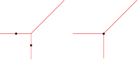
As a first simple example, consider the tropical analogue of a line in $\mathbb{P}^{2}$ meeting a point where it satisfies a $\psi$-class condition (equivalently in this case, where it has a specified tangent direction). This is the tropical line with incidence point in the trivalent vertex, see Figure 1.1. The reason from our point of view is as follows. Tropicalizing a stable log map yields the tropical curve as the dual intersection graph of the domain curve, and the valency of a vertex matches the number of special points (markings or nodes) of the corresponding curve component. Higher valencies thus give curve components more moduli (we see in Lemma LABEL:PsiGeomNew that the $\psi$-classes can essentially be pulled back from the moduli of the corresponding components of the domain, see also Prop. LABEL:psihat), and since a $\psi$-condition cuts down such moduli, a minimal valency is necessary for such a curve with $\psi$-conditions imposed on markings on that component to have a non-zero contribution.

A significant difference between log and ordinary GW invariants is the fact that $\psi$-classes in ordinary GW theory can be much more complicated, leading for example to the possibility of negative counts. A simple example is $\langle\ell\psi^{2}\rangle^{\mathbb{P}^{2}}_{0,\ell}$, i.e., the ordinary GW count of lines in $\mathbb{P}^{2}$ meeting a given generic line $\ell$ in a generic $\psi^{2}$-condition. Our tropical count ${}^{\operatorname{trop}}\langle\ell\psi^{2}\rangle^{\mathbb{P}^{2}}_{0,\ell}$ and hence our log invariant $\langle\ell\psi^{2}\rangle^{\mathbb{P}^{2}(\log D)}_{0,\ell}$ is $0$ here since satisfying the $\psi^{2}$ condition would require a four-valent vertex, and this is impossible for a tropical line in $\mathbb{P}^{2}$, see Fig. 1.1. However, $\langle\ell\psi^{2}\rangle^{\mathbb{P}^{2}}_{0,\ell}=-3$.

The discrepancy essentially arises because the log GW count considers extra markings at each point where the $\mathbb{P}^{1}$ meets the toric boundary $D$ of $\mathbb{P}^{2}$. By Thm. LABEL:main-comparison-thm, this log GW invariant can be related to the usual one by removing these extra markings via the divisor equation. Using our correspondence theorem Thm 1.1, we obtain

$$0\underset{\hbox{\tiny valency}\atop{\hbox{\tiny argument}}}{=}{}^{\operatorname{trop}}\langle\ell\psi^{2}\rangle^{\mathbb{P}^{2}}_{0,\ell}\underset{\hbox{\tiny correspondence}\atop{\hbox{\tiny theorem \ref{mainthmintro}}}}{=}\langle\ell\psi^{2}\rangle^{\mathbb{P}^{2}(\log D)}_{0,\ell}\underset{\hbox{\tiny divisor}\atop{\hbox{\tiny equation}}}{=}\langle\ell\psi^{2}\rangle^{\mathbb{P}^{2}}_{0,\ell}+3\underbrace{\langle[\operatorname{pt}]\psi^{1}\rangle^{\mathbb{P}^{2}}_{0,\ell}}_{=1}.$$

[GrP2] and [Over] describe more complicated tropical counts which do give the ordinary invariants for $\mathbb{P}^{2}$, but the geometric meaning of their counts was previously mysterious. The $3\langle[\operatorname{pt}]\psi^{1}\rangle^{\mathbb{P}^{2}}_{0,\ell}$-term above illustrates why some of their tropical curves appear. We plan to use our result to further illuminate their counts in a paper joint with N. Nabijou. We encourage the reader to look at the further Examples LABEL:example-double-psi, LABEL:Boundary-Markings and LABEL:ex-hyperell in §LABEL:sec-applications.

1.1. Statement of the main result

Let $X=X_{\Sigma}$ be a smooth projective toric variety given by a fan $\Sigma$ in $N_{\mathbb{R}}:=N\otimes_{\mathbb{Z}}\mathbb{R}$ for some $N\cong\mathbb{Z}^{n}$. A tropical degree $\Delta$ is a map $\Delta:I\rightarrow N$ for a finite index set $I$. For simplicity, let us assume here that each nonzero $\Delta(i)$ is contained in a ray of $\Sigma$. Let $D_{i}$ denote the boundary divisor corresponding to the ray through $\Delta(i)$. Denote $I^{\circ}:=\Delta^{-1}(\{0\})$ and $I^{\partial}:=I\setminus I^{\circ}$. Curves of degree $\Delta$ have marked points $(x_{i})_{i\in I}$ labelled by $I$. If $i\in I^{\partial}$, then $x_{i}$ is required to map to $D_{i}$ with intersection multiplicity equal to the index of $\Delta(i)$. For each $i\in I$, let $Z_{A_{i}}$ denote a generic regularly embedded closed subvariety of $X$ with tropicalization $A_{i}$. In particular, if $A_{i}\subset N_{\mathbb{R}}$ is an affine-linear subspace with rational slope, then $Z_{A_{i}}$ is the closure of a general orbit of the torus $\mathbb{G}(\operatorname{L}(A_{i})\cap N)\subset\mathbb{G}(N)$. For $i\in I^{\partial}$, let $Z_{A_{i},\Delta(i)}$ denote $Z_{A_{i}}\cap D_{i}$.

On the tropical side, corresponding to a degree $\Delta$ curve $C$ (with log structure) is a tropical curve $h:\Gamma\rightarrow N_{\mathbb{R}}$. Here, $\Gamma$ is the dual graph to $C$, with marked points $x_{i}$ of $C$ corresponding to half-edges $E_{i}$ of $\Gamma$. The edges of $\Gamma$ are equipped with non-negative integer weights. Weight $0$ edges are contracted by the map $h$, while the other edges are embedded into lines with rational slope. Furthermore, $h$ satisfies a “balancing condition” and has degree $\Delta$, meaning that for each $i\in I$, $h(E_{i})$ points in the direction $\Delta(i)$, and $E_{i}$ has weight equal to the index of $\Delta(i)$. The genus of $\Gamma$ is equal to its first Betti number (plus the sum of the genera of the vertices of $\Gamma$, but these are $0$ for non-superabundant cases). We say $h:\Gamma\rightarrow N_{\mathbb{R}}$ satisfies ${\bf A}:=(A_{i})_{i\in I}$ if $h(E_{i})\subset A_{i}$ for each $i$. For $\Psi:=(s_{i})_{i\in I^{\circ}}$ a tuple of non-negative integers $s_{i}$, we say $\Gamma$ satisfies $\Psi$ if

$$\operatorname{val}(V)-3\geq\sum_{\begin{subarray}{c}i\in I^{\circ}\\ E_{i}\ni V\end{subarray}}s_{i}$$

for each vertex $V$. We say $\Gamma$ is non-superabundant if its vertices all have genus $0$ and if its space of deformations locally has dimension $|I|+(n-3)(1-g)$.

By [ACGS, Thm. 1.1.2], a log Gromov-Witten invariant decomposes into types of tropical curves. In particular, given a degeneration, we can decompose into the contribution from superabundant and non-superabundant curves (see Def. 2.3), in notation $\langle..\rangle={}^{s}\langle..\rangle+{}^{\operatorname{ns}}\langle..\rangle$. It follows from Prop. 2.5 that ${}^{s}\langle..\rangle=0$ when $g=0$, or for any $g$ with $n\leq 2$ and no $\psi$-conditions, and also in many $n=1$ cases with limited $\psi$-classes (including the Hurwitz counts of §LABEL:section-hurwitz). On the other hand, (3) and (4) of Remark 2.6 show that superabundant tropical curves probably appear in most other cases, although it was recently shown [CJMR2, Thm. 3.9] for stationary invariants of Hirzebruch surfaces that even though superabundant curves might exists, ${}^{s}\langle..\rangle$ still equals $0$. A general statement about superabundant curves is beyond current knowledge.

Theorem 1.1.

Let $g\geq 0$ and $\{s_{i}\geq 0\}_{i\in I^{\circ}}$ be given and assume that

$$\sum_{i\in I}\operatorname{codim}A_{i}+\sum_{i\in I^{\circ}}s_{i}=|I|+(n-3)(1-g).$$

There exists a log smooth toric degeneration $X_{0}(\log D_{0})$ of $X(\log D)$ such that the following are non-negative rational numbers that coincide:

1. The non-superabundant part of the log Gromov-Witten invariant

   $${}^{\operatorname{ns}}\langle\{[Z_{A_{i}}]\psi^{s_{i}}\}_{i\in I^{\circ}},\{[Z_{A_{i},\Delta(i)}]\}_{i\in I^{\partial}}\rangle^{X_{0}(\log D_{0})}_{g,\Delta},$$

2. The count with multiplicities (cf. (LABEL:MultGamma), or more generally (LABEL:GeneralMultGamma)) of rigid marked tropical curves having genus $g$ and degree $\Delta$ satisfying ${\bf A}=(A_{i})_{i\in I}$ and $\Psi=(s_{i})_{i\in I^{\circ}}$.

If ${}^{s}\langle..\rangle=0$ then these numbers also coincide with $\langle\{[Z_{A_{i}}]\psi^{s_{i}}\}_{i\in I^{\circ}},\{[Z_{A_{i},\Delta(i)}]\}_{i\in I^{\partial}}\rangle^{X(\log D)}_{g,\Delta}$.

Proof.

The equality (1)=(2) is Theorem LABEL:MainThm and Theorem LABEL:MainThmExtended. (2) is easily non-negative rational. ∎

A curve in $X$ is called torically transverse if it meets no toric strata of codimension greater than one.

Theorem 1.2.

In the absence of automorphisms of the tropical curves in (2), (e.g. for $g=0$, see Remark 2.2) the count of (1) and (2) furthermore coincides with the non-negative integer-valued count of non-superabundant torically transverse curves in $X_{0}(\log D_{0})$ (or in $X(\log D)$ if ${}^{s}\langle..\rangle=0$) of genus $g$ and degree $\Delta$ meeting $Z_{A_{i}}$ at a marked point with a generic $\psi^{s_{i}}$-condition for each $i\in I^{\circ}$, and meeting $D_{i}$ in $Z_{A_{i}}$ with tangency order equal to the index of $\Delta(i)$ for each $i\in I^{\partial}$. In general, these naive algebraic counts must actually be weighted by $1$ over the numbers of automorphisms of the corresponding marked tropical curves.

Remark 1.3.

We note that the log curves contributing to (1) in Theorem 1.1 have unobstructed deformations by Proposition LABEL:VirtualActual, so they deform to contribute the same amount to the log Gromov-Witten numbers in the nearby fibers. In the absence of superabundant curves, this is also what leads to the equality with $\langle\{[Z_{A_{i}}]\psi^{s_{i}}\}_{i\in I^{\circ}},\{[Z_{A_{i},\Delta(i)}]\}_{i\in I^{\partial}}\rangle^{X(\log D)}_{g,\Delta}$.

Proof of Thm. 1.2.

The count in (1) arises via an intersection cycle $\gamma$ composed (in the case of trivial $\operatorname{Aut}(\Gamma)$) of reduced non-stacky points parametrizing torically transverse curves (Prop. LABEL:PreCount combined with Lemma LABEL:LogStructureCounts, plus Lemma LABEL:NoAut for the non-stackiness). The assertion follows because this cycle is the Gysin restriction of a cycle of stable maps of the total space of the degeneration constructed in §LABEL:sec-tordeg, and toric transversality is an open condition and stackiness a closed condition. ∎

1.2. Notation

Let $\Bbbk$ be an algebraically closed field of characteristic $0$. Fix an $n\in\mathbb{Z}_{>0}$, and let $N$ denote a free Abelian group of rank $n$. Denote $N_{\mathbb{Q}}:=N\otimes_{\mathbb{Z}}\mathbb{Q}$ and $N_{\mathbb{R}}:=N\otimes_{\mathbb{Z}}\mathbb{R}$. For a subset $A\subset N_{\mathbb{Q}}$, $\operatorname{L}(A)$ denotes the linear subspace spanned by differences $u-v$ of points in $A$. In particular, if $A$ is an affine subspace, $\operatorname{L}(A)$ is the linear subspace parallel to $A$. We write $\operatorname{L}_{N}(A)$ for $\operatorname{L}(A)\cap N$. Denote $\lx@glossaries@gls@link{main}{N^{\prime}}{\leavevmode N^{\prime}}:=N\oplus\mathbb{Z}$, $\lx@glossaries@gls@link{main}{M}{\leavevmode M}:=\operatorname{Hom}(N,\mathbb{Z})$, $\lx@glossaries@gls@link{main}{M^{\prime}}{\leavevmode M^{\prime}}:=\operatorname{Hom}(N^{\prime},\mathbb{Z})$. Let $\lx@glossaries@gls@link{main}{CA}{\leavevmode\operatorname{C}(A)}:=\overline{\{(ta,t)|a\in A,t\in\mathbb{Q}_{\geq 0}\}}\subset N^{\prime}_{\mathbb{Q}}$ denote the closed cone over $A$. In particular, $\lx@glossaries@gls@link{main}{LCA}{\leavevmode\operatorname{LC}(A)}:=\operatorname{L}(\operatorname{C}(A))$ denotes the linear closure of $A\times\{1\}$ in $N_{\mathbb{Q}}\times\mathbb{Q}$. For a ${\mathbb{Z}}$-module $V$, we set ${\mathbb{G}}(V)={\mathbb{G}}_{m}(\Bbbk)\otimes_{\mathbb{Z}}V$.

For any scheme $Y$ we will write $Y^{\dagger}$ to denote $Y$ equipped with a log structure. Similarly, a morphism of log schemes will be given a $\dagger$ in its superscript. We will sometimes use Witten’s correlator notation for Gromov-Witten invariants $\langle insertions\rangle^{X}_{g,\beta}$ and similarly for log Gromov-Witten invariants $\langle insertions\rangle^{X(\log D)}_{g,\Delta}$ for the divisorial log structure of a divisor $D$ on $X$. For the latter, note that the refined degree $\Delta$ contains information about the orders of tangencies and numbers of markings that go to each component of $D$.

For the reader’s convenience, we will keep track of important notation from §2-§LABEL:Sing in the glossary below.

Glossary

${\bf A}$

An affine constraint, i.e., a tuple $(A_{i})_{i\in I}$ of affine subspaces of $N_{\mathbb{Q}}$

$\operatorname{Aut}(\Gamma)$

Automorphism group of the tropical curve $(\Gamma,\epsilon,h)$

$\operatorname{C}(A)$

Closed cone $\overline{\{(ta,t)|a\in A,t\in\mathbb{Q}_{\geq 0}\}}\subset N^{\prime}_{\mathbb{Q}}$ over $A$

$\Delta$

Degree of a type $(\Gamma,\epsilon,u)$, i.e., the map taking $i\in I$ to $\Delta(i):=w(E_{i})u_{i}\in N$

$d^{\operatorname{trop}}_{g,\Delta}$

Expected tropical dimension $e_{\infty}+(n-3)(1-g)$

$\overline{e}$

$\#\Gamma^{[1]}_{c}$, i.e., the number of compact edges of $\Gamma$

$e_{\infty}$

$\#I$, or equivalently, $\#\Gamma^{[1]}_{\infty}$

$\epsilon$

Marking $I\buildrel\sim\over{\hbox{$\longrightarrow$}}\Gamma^{[1]}_{\infty}$ for some index-set $I$. We often write $\epsilon(i)$ as $E_{i}$

$F\Gamma$

Set of flags $(V,E)$ of $\Gamma$

$g$

Genus-function $\Gamma^{[0]}\rightarrow\mathbb{Z}_{\geq 0}$. We typically write $g(v)$ as $g_{V}$

$\Gamma$

Complement of some subset of the $1$-valent vertices of $\overline{\Gamma}$

$\Gamma^{[0]}$

Vertices of $\Gamma$

$\Gamma^{[1]}$

Edges of $\Gamma$

$\Gamma^{[1]}_{c}$

Compact edges of $\Gamma$

$\Gamma^{[1]}_{\infty}$

Non-compact edges of $\Gamma$

$\overline{\Gamma}$

Topological realization of a finite connected graph

$(\Gamma,\epsilon)$

Data of $\Gamma$, the weight-function $w$ and genus-function $g$, and the marking $\epsilon$

$g(\Gamma)$

Genus of $\Gamma$, defined as $b_{1}(\Gamma)+\sum_{V\in\Gamma^{[0]}}g_{V}$

$h$

Map $\Gamma\rightarrow N_{\mathbb{R}}$ from the data of a parametrized marked tropical curve

$I^{\circ}$

Set of $i\in I$ for which $w(E_{i})=0$. I.e., the interior markings

$I^{\partial}$

Set of $i\in I$ for which $w(E_{i})\neq 0$. I.e., the boundary markings

$I_{V}^{\circ}$

Set of $i\in I^{\circ}$ such that $E_{i}$ contains the vertex $V$

$\Bbbk$

Fixed algebraically closed field of characteristic zero

$\operatorname{L}(A)$

Linear subspace of $N_{\mathbb{Q}}$, translate of the affine subspace $A\subset N_{\mathbb{Q}}$ to the origin

$\operatorname{LC}(A)$

$\operatorname{L}(\operatorname{C}(A))$

$\operatorname{L}_{N}(A)$

$\operatorname{L}(A)\cap N$

$M$

Dual lattice of $N$

$m_{V}$

$\#I_{V}^{\circ}$, i.e., the number of weight-zero non-compact edges containing $V$

$N$

Free Abelian group of finite rank $n$

$\operatorname{ov}(\Gamma)$

Over-valence $\sum_{V\in\Gamma^{[0]}}\operatorname{ov}(V)$ of $\Gamma$

$\operatorname{ov}(V)$

Over-valence $\operatorname{val}(V)-3$ of a vertex $V$

$\Phi_{\mathbb{Q}}$

Map given in (8)

$\Psi$

A tuple $(s_{i})_{i\in I^{\circ}}\in\mathbb{Z}_{\geq 0}^{|I^{\circ}|}$ indicating the $\psi$-class conditions

$(\Gamma,\epsilon,h)$

Parametrized marked tropical curve, or the (marked) tropical curve it represents

$\mathfrak{T}_{g,\Delta}({\bf A},\Psi)$

Space of tropical curves of genus $g$ and degree $\Delta$ satisfying ${\bf A}$ and $\Psi$

$\mathfrak{T}^{\operatorname{ns}}_{g,\Delta}({\bf A},\Psi)$

Non-superabundant elements of $\mathfrak{T}_{g,\Delta}({\bf A},\Psi)$

$\mathfrak{T}_{(\Gamma,\epsilon,u)}$

Space of marked tropical curves of type $(\Gamma,\epsilon,u)$

$u_{E}$

Simplified notation for $u_{(V,E)}$ when the choice of $V\in E$ is clear from context or unimportant

$u_{i}$

Simplified notation for $u_{(V,E_{i})}$, where $V$ is the unique vertex of the non-compact edge $E_{i}$

$u_{(V,E)}$

Primitive integral vector emanating from $h(V)$ into $h(E)$, or $0$ if $h(E)$ is a point

$\operatorname{val}(V)$

Valence of a vertex $V$, counting self-adjacent edges twice

$w$

Weight-function $\Gamma^{[1]}\rightarrow\mathbb{Z}_{\geq 0}$

1.3. Acknowledgements

The authors are grateful to Mark Gross for suggesting the Nishinou-Siebert approach to descendant Gromov-Witten invariants. We thank Bernd Siebert for encouraging the use of log GW theory and answering questions. We also thank Y.P. Lee in this context. We thank Tony Yue Yu, Rahul Pandharipande and Bernd Siebert for inspiring us to view $\psi$-classes as being pulled back from the underlying moduli space of stable curves rather than our early approach of using tangency conditions. We thank Peter Overholser for his repeated warnings about negative counts and useful examples he gave. We thank Mark Gross, Andreas Gross, Hannah Markwig and Renzo Cavalieri for explaining their related projects. David Rydh gave a useful answer to a question on Chow groups for stacks. We thank the anonymous referee for suggesting various improvements.

2. Tropical curves

We follow [Mi, NS]. While definitions in this section might appear ad hoc, we will later see in §LABEL:tropicalization that the herein defined objects are natural because they are the output of tropicalization.

Let ¯Γ denote the topological realization of a finite connected graph. Let Γ be the complement of some subset of the $1$-valent vertices of $\overline{\Gamma}$. Let Γ[0], Γ[1], Γ[1]∞, and Γ[1]c denote the the sets of vertices, edges, non-compact edges, and compact edges of $\Gamma$, respectively. We equip $\Gamma$ with a “weight-function” $\lx@glossaries@gls@link{main}{w}{\leavevmode w}:\Gamma^{[1]}\rightarrow\mathbb{Z}_{\geq 0}$ and a “genus-function” $\lx@glossaries@gls@link{main}{g}{\leavevmode g}:\Gamma^{[0]}\rightarrow\mathbb{Z}_{\geq 0}$ (typically writing $g(V)$ as $g_{V}$), and we require that univalent and bivalent vertices have positive genus. A marking of $\Gamma$ is a bijection $\lx@glossaries@gls@link{main}{eps}{\leavevmode\epsilon}:I\rightarrow\Gamma^{[1]}_{\infty}$ for some index set $I$.

Denote $E_{i}:=\epsilon(i)$. We let $\lx@glossaries@gls@link{main}{Icirc}{\leavevmode I^{\circ}}:=\epsilon^{-1}(w^{-1}(0))\subset I$, i.e., the set of $i\in I$ for which $w(E_{i})=0$, and we call these the interior markings. The complement $\lx@glossaries@gls@link{main}{Ip}{\leavevmode I^{\partial}}=I\setminus I^{\circ}$ forms the boundary markings. Denote by (Γ,ϵ) the data of $\Gamma$, the weight-function $w$ and genus-function $g$ (left out of the notation), and the marking. Let $\lx@glossaries@gls@link{main}{einf}{\leavevmode e_{\infty}}:=\#I$. For each vertex $V$, we let IV∘ denote the set of $i\in I^{\circ}$ such that $V\in E_{i}$, and let $\lx@glossaries@gls@link{main}{mV}{\leavevmode m_{V}}:=\#I_{V}^{\circ}$. We call $V$ marked if $m_{V}>0$ and unmarked if $m_{V}=0$.

Definition 2.1.

A parametrized marked tropical curve $(\Gamma,\epsilon,h)$ is data $(\Gamma,\epsilon)$ as above, along with a continuous map $\lx@glossaries@gls@link{main}{h}{\leavevmode h}:\Gamma\rightarrow N_{\mathbb{R}}$ such that

1. For each edge $E\in\Gamma^{[1]}$, $h|_{E}$ is constant if and only if $w(E)=0$. Otherwise, $h|_{E}$ is a proper embedding into an affine line with rational slope. We will refer to edges $E$ with $w(E)=0$ as contracted edges. In particular, self-adjacent edges (those with the same vertex at both ends) must have weight zero as there is no way to embed a loop into a line.

2. For every $V\in\Gamma^{[0]}$, $h(V)\in N_{\mathbb{Q}}$, and the following balancing condition holds. For any edge $E\ni V$, denote by u(V,E) the primitive integral vector emanating from $h(V)$ into $h(E)$ (or $u_{(V,E)}:=0$ if $h(E)$ is a point). Then

   $$\sum_{E\ni V}w(E)u_{(V,E)}=0.$$

Furthermore, for each contracted edge $E$, we have the additional data of a length $\ell(E)\in\mathbb{Q}_{>0}$. For the purposes of this paper, we assume that $h$ is non-constant, or equivalently, that $e_{\infty}>0$. Also, to simplify the exposition, we assume throughout that $\Gamma^{[0]}\neq\emptyset$, and we handle this case separately in Remark LABEL:NoVertices.

For non-compact edges $E_{i}\ni V$, we may denote $u_{(V,E_{i})}$ simply as $u_{E_{i}}$ or ui (with $u_{i}=0$ if $E_{i}$ is contracted). Similarly, for any edge $E$, we may simply write uE when the vertex is either clear from context or unimportant, e.g., as in $\mathbb{Z}u_{E}$.

An isomorphism of marked parametrized tropical curves $(\Gamma,\epsilon,h)$ and $(\Gamma^{\prime},\epsilon^{\prime},h^{\prime})$ is a homeomorphism $\Phi:\Gamma\rightarrow\Gamma^{\prime}$ respecting the weights, markings, and lengths such that $h=h^{\prime}\circ\Phi$. A marked tropical curve (or, for short, a tropical curve) is then defined to be an isomorphism class of parametrized marked tropical curves. We will use $(\Gamma,\epsilon,h)$ to denote the isomorphism class it represents and will often abbreviate this as simply $h$ or $\Gamma$. We will denote the automorphism group of the tropical curve represented by $(\Gamma,\epsilon,h)$ as Aut(Γ).

Remark 2.2.

Since unbounded edges are marked, we note that $\operatorname{Aut}(\Gamma)$ is always trivial for $g=0$. More generally, if no two distinct vertices map to the same point, then automorphisms can only act by permuting edges that have the same vertices, and by Lemma 2.4, curves with such collections of edges are superabundant unless $n=1$. Example LABEL:ex-hyperell features nontrival $\operatorname{Aut}(\Gamma)$. Note that after the removal of boundary markings, automorphisms may occur also for $g=0$ and any $n$, cf. §LABEL:OrdinaryGW.

A tropical immersion is a tropical curve with no higher-genus vertices, no self-adjacent edges, and no pairs of edges which share a vertex and point in the same direction.

If $b_{1}(\Gamma)$ denotes the first Betti number of $\Gamma$, the genus of a tropical curve $\Gamma$ is defined as

$$\lx@glossaries@gls@link{main}{gGamma}{\leavevmode g(\Gamma)}=b_{1}(\Gamma)+\sum_{V\in\Gamma^{[0]}}g_{V}.$$

Set $\lx@glossaries@gls@link{main}{ebar}{\leavevmode\overline{e}}:=\#\Gamma^{[1]}_{c}$, so $\bar{e}+e_{\infty}$ is the total number of edges of $\Gamma$. Let val(V) denote the valence of a vertex $V$ (counting self-adjacent edges twice). Motivated by considering a valency of three to be generic, one defines the over-valence $\lx@glossaries@gls@link{main}{ovV}{\leavevmode\operatorname{ov}(V)}:=\operatorname{val}(V)-3$, and

$$\lx@glossaries@gls@link{main}{ovG}{\leavevmode\operatorname{ov}(\Gamma)}:=\sum_{V\in\Gamma^{[0]}}\operatorname{ov}(V).$$

Now assume $g_{V}=0$ for every $V\in\Gamma^{[0]}$. Note that $\operatorname{ov}(V)\geq 0$ for all $V\in\Gamma^{[0]}$. Let FΓ denote the set of flags $(V,E)$, $V\in E$, of $\Gamma$ (with self-adjacent edges contributing twice). Computing $\#F\Gamma$ once via vertices, once via edges, yields

(1) $$3\#\Gamma^{[0]}+\operatorname{ov}(\Gamma)=e_{\infty}+2\overline{e}.$$

A computation of the Euler characteristic of $\Gamma$ yields $1-g=\#\Gamma^{[0]}-\overline{e}$. Using this to eliminate $\#\Gamma^{[0]}$ in (1) gives

(2) $$e_{\infty}=\overline{e}-3g+3+\operatorname{ov}(\Gamma).$$

The type of a marked tropical curve (possibly with positive $g_{V}$’s) is the data $(\Gamma,\epsilon)$ (including the weights and $g_{V}$’s and up to homeomorphism respecting this data and the markings), along with the data of the map $u:F\Gamma\rightarrow N$, $(V,E)\mapsto u_{(V,E)}$. Let T(Γ,ϵ,u) denote the space of marked tropical curves of type $(\Gamma,\epsilon,u)$. We may write $\mathfrak{T}_{\Gamma}$ for short. If $\Gamma$ is genus $0$, we have

(3) $$\mathfrak{T}_{(\Gamma,\epsilon,u)}\cong N_{\mathbb{Q}}\times\mathbb{Q}_{>0}^{\overline{e}}.$$

Indeed, we can specify $h\in\mathfrak{T}_{(\Gamma,\epsilon,u)}$ by specifying the image in $N_{\mathbb{Q}}$ of some $V\in\Gamma^{[0]}$ and then specifying the lengths of the compact edges. With a similar approach, we obtain more generally for curves of any genus that

(4) $$\mathfrak{T}_{(\Gamma,\epsilon,u)}\cong N_{\mathbb{Q}}\times(\mathbb{Q}_{>0}^{\overline{e}}\cap W),$$

where $W$ is the subspace of $\mathbb{Q}^{\overline{e}}$ generated by vectors of the form $(a_{E})_{E\in\Gamma^{[1]}_{c}}$ such that for all closed loops in $\Gamma$, if $L$ is the set of edges of such a loop, we have

$$0=\sum_{E\in L}a_{E}u_{E}.$$

Here, a loop in $\Gamma$ is defined to be a cyclically ordered sequence of edges $(E_{1},...,E_{r})$ in $\Gamma$, equipped with orientations with respect to which the starting point of $E_{i+1}$ is the ending point of $E_{i}$ for each $i=1,\ldots,r$. The directions of the $u_{E}$’s above are chosen to respect this orientation. $W$ is thus the constraint to have the loops close up. As we will see, the dimension of $W$ and hence of $\mathfrak{T}_{(\Gamma,\epsilon,u)}$ can vary even for fixed $n$, $\overline{e}$, and $g$. The maximal codimension $W$ can have is $gn$, so (4) motivates the following definition.

Definition 2.3.

A tropical curve $\Gamma$ is called superabundant if it contains at least one vertex of positive genus, or if every vertex is genus $0$ but the inequality $\dim\mathfrak{T}_{(\Gamma,\epsilon,u)}\geq n+\overline{e}-ng$ is strict (i.e. not an equality).

Assume again that $g_{V}=0$ for each $V$. The span of a loop is defined to be the span of the directions of its edges. One easily sees the following sufficient condition for superabundance:

Lemma 2.4.

If $\Gamma$ has a loop that does not span $N_{\mathbb{Q}}$, then $\Gamma$ is superabundant. In particular, non-superabundant curves have no self-adjacent edges.

See Fig. 2.2 for an example demonstrating that the converse of Lemma 2.4 is false. We do, however, have the following partial converses:

Proposition 2.5.

For g=0, all tropical curves are non-superabundant. If $n=1$, all tropical curves without self-adjacent edges are non-superabundant. For $n=2$, all tropical immersions for which $\operatorname{val}(V)>3$ holds at most at one vertex are non-superabundant.

Proof.

All the statements are easily checked except the last one for $n=2$. This is essentially [Mi, Prop. 2.23], noting that the vertex with $V$ with $\operatorname{val}(V)>3$ can be chosen as the start for Mikhalkin’s inductive construction of a maximal ordered tree in the curve. ∎

Remark 2.6.

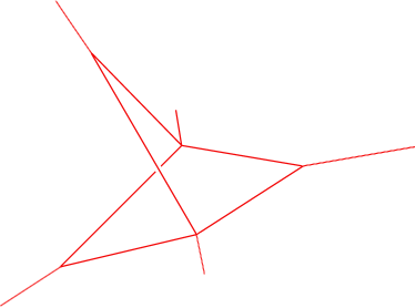
1. A typical example for a superabundant $g=1$, $n=2$ curve with no contracted edges is the following curve supported on a line (a sequence of a weight $2$ edge, double edge, weight $2$ edge):

2. Mikhalkin provides an example for a superabundant tropical immersion for $n=2,g=22$, [Mi, Rem. 2.25] based on Pappus theorem. An $n=2$, $g=3$ superabundant immersion is given in [GM07, Example 3.10].

3. Superabundant curves of any higher genus can be generated from genus zero curves by attaching self-adjacent edges (or similarly, by replacing an unmarked trivalent vertex by a triangle of edges, or by inserting curves like from (1) above into edges with weight greater than $1$). Since we generally want to avoid superabundancy, this observation is particularly problematic if $n\geq 3$ because then the expected dimension $d^{\operatorname{trop}}_{g,\Delta}$ (see (10)) increases or (for $n=3$) stays the same as we decrease $g$. Hence, given some fixed constraints to be met for some degree (constraints and degrees will be introduced below), it should be at least as easy to find curves satisfying these constraints in genus zero as in higher genus, and then from such curves we can attach self-adjacent edges (or apply the other modifications we just described) to increase the genus. One therefore expects that for $n\geq 3$ and $g>0$, superabundant curves are abundant.

4. For $n=2$, increasing $g$ by $1$ only increases the expected dimension $d^{\operatorname{trop}}_{g,\Delta}$ by $1$. So if one considers a rigid collection of conditions for given $g>0$ and $\Delta$ and then forgets a $\psi$-class (i.e., decreases one of the $s_{i}$’s in (6) below by $1$), one would expect there to be a $0$-dimensional collection of curves of genus $g-1$ which satisfy the modified conditions. Given such a genus $g-1$ curve, one could then insert a self-adjacent edge at the vertex where the psi-class was forgotten to get a superabundant curve of the desired genus which satisfies the original collection of conditions (these are not tropical immersions, so Prop. 2.5 does not apply). So even in dimension $2$, it seems that higher-genus counts with $\psi$-class insertions will typically involve the appearance of superabundant curves, as previously noted in [Bou, Appx. B]. However, in at least some cases, the contributions of the superabundant curves is trivial, e.g., for stationary invariants of Hirzebruch surfaces according to [CJMR2, Thm. 3.9].

Figure 2.2. A tropical genus two curve in ${\mathbb{R}}^{3}$ that is superabundant even though all its loops span.

Allow $g_{V}>0$ again. The degree Δ of a type $(\Gamma,\epsilon,u)$ is the data of the index set $I$, along with the map

(5) $$\Delta:I\rightarrow N,\hskip 36.135pt\Delta(i):=w(E_{i})u_{i}.$$

Note that the data of $I$ (hence of $e_{\infty}$) is part of the data of the degree $\Delta$ but is suppressed in the notation.

Lemma 2.7 ([NS], Proposition 2.1).

The number of types of tropical curves of fixed degree, fixed number of markings, and fixed genus is finite.

2.1. Incidence and $\psi$-class conditions

Here we consider only “affine constraints.” See §LABEL:GenInc for a discussion of how to generalize to other tropical constraints.

Definition 2.8.

An affine constraint A for the degree $\Delta$ is a tuple $(A_{i})_{i\in I}$ of affine subspaces of $N_{\mathbb{Q}}$ such that $\Delta(i)\in\operatorname{L}(A_{i})$ for each $i$. A marked tropical curve $(\Gamma,\epsilon,h)$ matches the constraints ${\bf A}$ if $h(E_{i})\subset A_{i}$ for each $i\in I$.

Consider another tuple $\lx@glossaries@gls@link{main}{Psi}{\leavevmode\Psi}:=(s_{i})_{i\in I^{\circ}}\in\mathbb{Z}_{\geq 0}^{|I^{\circ}|}$. We say $(\Gamma,\epsilon,h)$ satisfies $\Psi$ if for each vertex $V$ with $g_{V}=0$, we have

(6) $$\operatorname{ov}(V)\geq\sum_{i\in I_{V}^{\circ}}s_{i}.$$

We are interested in the space

of marked tropical curves of genus $g$ and degree $\Delta$, matching the constraints ${\bf A}$ and satisfying the $\psi$-class conditions $\Psi$.

For a marked vertex $V\in\Gamma^{[0]}$ such that $g_{V}=0$ and (6) is an equality, let $I_{V}^{\circ}=\{i_{1},\ldots,i_{m_{V}}\}$, and then let ⟨V⟩ denote the multinomial coefficient

(7) $$\langle V\rangle:=\binom{\operatorname{ov}(V)}{s_{i_{1}},\ldots,s_{i_{m_{V}}}}:=\frac{\operatorname{ov}(V)!}{\prod_{i\in I_{V}^{\circ}}s_{i}!}.$$

For unmarked $V$, $\langle V\rangle:=1$. We won’t need an analog for higher-genus vertices in this paper.

The factor $\langle V\rangle$ will contribute to the multiplicity with which we will count tropical curves. Example LABEL:example-double-psi demonstrates this. Note that $\langle V\rangle=1$ whenever $m_{V}=1$ and (6) is an equality, and consequently, $\langle V\rangle=1$ holds generically for all vertices when there are no $\psi$-classes. As we will see, the reason for this multiplicity $\langle V\rangle$ is that it is equal to $\int_{[\overline{\mathcal{M}}_{0,\operatorname{val}(V)}]}\prod_{i\in I_{V}^{\circ}}\psi_{i}^{s_{i}}$ (cf. [Kock, Lemma 1.5.1]).

Recall that for any affine subspace $A$, we write $\operatorname{L}(A)$ for the linear subspace parallel to $A$. The following proposition describes the subspaces of $\mathfrak{T}_{g,\Delta}({\bf A},\Psi)$ corresponding to curves of a fixed type. We first state an elementary lemma that it uses.

Lemma 2.9.

Given two affine subspaces $A_{1},A_{2}\subset N_{\mathbb{Q}}$, if $A^{\prime}_{1}$ is a general translate of $A_{1}$ then the intersection $A^{\prime}_{1}\cap A_{2}$ is either empty or transverse (i.e. $\operatorname{codim}A^{\prime}_{1}\cap A_{2}=\operatorname{codim}A_{1}+\operatorname{codim}A_{2}$).

Proposition 2.10.

Let $(\Gamma,\epsilon,h)\in\mathfrak{T}_{g,\Delta}({\bf A},\Psi)$. For each edge $E\in\Gamma^{[1]}_{c}$, fix a labeling of its two vertices as $\partial^{+}E$ and $\partial^{-}E$. For $E\in\Gamma^{[1]}_{\infty}$, define $\partial E$ to be the unique vertex contained in $E$. Define a map of vector spaces

(8) $$\lx@glossaries@gls@link{main}{PhiQ}{\leavevmode\Phi_{\mathbb{Q}}}:\prod_{V\in\Gamma^{[0]}}N_{\mathbb{Q}} \rightarrow\left(\prod_{E\in\Gamma^{[1]}_{c}}N_{\mathbb{Q}}/\mathbb{Q}u_{E}\right)\times\left(\prod_{i\in I}N_{\mathbb{Q}}/\operatorname{L}(A_{i})\right)$$

$$H \mapsto((H_{\partial^{+}E}-H_{\partial^{-}E})_{E\in\Gamma^{[1]}_{c}},(H_{\partial E_{i}})_{i\in I})$$

Then the space of tropical curves in $\mathfrak{T}_{g,\Delta}({\bf A},\Psi)$ of the same combinatorial type $u$ as $(\Gamma,\epsilon,h)$ can be identified with a non-empty open convex polyhedron (i.e., an intersection of finitely many open affine half-spaces in $\ker(\Phi_{\mathbb{Q}})$. Furthermore, assuming that the constraints are in general position (in the space of possible translations of the constraints), and that $g_{V}=0$ for each $V$, the dimension of this space is

$$\dim[\ker(\Phi_{\mathbb{Q}})]=\dim\mathfrak{T}_{(\Gamma,\epsilon,u)}-\sum_{i\in I}\operatorname{codim}(A_{i}).$$

If $\Gamma$ is not superabundant, this becomes

$$\dim[\ker(\Phi_{\mathbb{Q}})]=n+\overline{e}-ng-\sum_{i\in I}\operatorname{codim}(A_{i}).$$

Proof.

Points $H=(H_{V})_{V}$ on the left-hand side of (8) give deformations of $h$ by adding $H_{V}$ to $h(V)\in N_{\mathbb{Q}}$. For $E\in\Gamma^{[1]}_{c}$, $h(E)$ is deformed to be the line segment connecting $h(\partial^{\pm}E)+H_{\partial^{\pm}E}$. The image of an unbounded edge $E$ is deformed to $(h(E)+H_{\partial E})$. By construction, these are the deformations of $h$ which still embed edges into affine lines of rational slope or contract them, but the balancing conditions and constraints may not hold. The deformed curve corresponding to some $H$ will have the original combinatorial type (and in particular be balanced) if and only if $H$ is in the kernel of the first factor of $\Phi_{\mathbb{Q}}$ and, for each $E\in\Gamma^{[1]}_{c}$, the deformed edge vector $((h(\partial^{+}E)+H_{\partial^{+}E})-(h(\partial^{-}E)+H_{\partial^{-}E}))$ is a positive multiple of the original one $h(\partial^{+}E)-h(\partial^{-}E)$ (this is an open affine half-space condition). Similarly, it will satisfy the incidence conditions if and only if $H$ is in the kernel of the second factor. This proves the first claim.

We prove the second claim by induction. If there are no incidence conditions (i.e., each $A_{i}$ equals $N_{\mathbb{Q}}$) then the claim is trivial. Let $P$ be a small generic translate of $\ker(\Phi_{\mathbb{Q}})$ corresponding to the subspace of deformations of $h$ which satisfy all the conditions we have imposed so far (with the open half-space conditions removed since we are only interested in dimensions right now). Suppose we add a constraint $A_{i}+\epsilon$, where $\epsilon$ is a small generic element of $N_{\mathbb{Q}}$. This adds a factor $N_{\mathbb{Q}}/\operatorname{L}(A_{i})$ to the right-hand side, and an element $H$ in the domain of $\Phi_{\mathbb{Q}}$ maps to $0$ in this factor if and only if $H_{i}\in\operatorname{L}(A_{i})+\epsilon$. This corresponds to intersecting $P$ with $(\operatorname{L}(A_{i})+\epsilon)$. By Lemma 2.9, these intersections are transverse, so this proves the claim.

Finally, the claim for the non-superabundant case follows from Def. 2.3. ∎

Lemma 2.11.

For ${\bf A}$ generic and $(\Gamma,\epsilon,h)\in\mathfrak{T}_{g,\Delta}({\bf A},\Psi)$ non-superabundant, $\Phi_{\mathbb{Q}}$ is surjective.

Proof.

Prop. 2.10 gives the rank of the kernel, so to show that the rank of the cokernel of $\Phi_{\mathbb{Q}}$ vanishes we may compute $\dim\operatorname{coker}(\Phi_{\mathbb{Q}})=\dim\ker\Phi_{\mathbb{Q}}+\dim\operatorname{codomain}(\Phi_{\mathbb{Q}})-\dim\operatorname{domain}\Phi_{\mathbb{Q}}$ giving

$$\left(n+\overline{e}-ng-\sum_{i}\operatorname{codim}(A_{i})\right)+\left((n-1)\overline{e}+\sum_{i}\operatorname{codim}(A_{i})\right)-n\#\Gamma^{[0]}$$

which is seen to vanish by inserting $\#\Gamma^{[0]}=\overline{e}+1-g$. ∎

Note that for non-superabundant $(\Gamma,\epsilon,h)\in\mathfrak{T}_{g,\Delta}({\bf A},\Psi)$ with each $g_{V}=0$, it follows from (6) that

(9) $$\operatorname{ov}(\Gamma)\geq\sum_{i\in I^{\circ}}s_{i}.$$

Definition 2.12.

Fix a genus $g$, a degree $\Delta$, and a tuple $\Psi$ as above. An affine constraint ${\bf A}$ of codimension ${\bf a}$ is general for $\Delta$ and $\Psi$ if

(10) $$\sum_{i\in I^{\circ}}s_{i}+\sum_{i\in I}\operatorname{codim}(A_{i})=\lx@glossaries@gls@link{main}{dtrop}{\leavevmode d^{\operatorname{trop}}_{g,\Delta}}:=e_{\infty}+(n-3)(1-g),$$

and for any non-superabundant $(\Gamma,\epsilon,h)\in\mathfrak{T}_{g,\Delta}({\bf A},\Psi)$ with each $g_{V}=0$, (9) is an equality and $\Gamma$ has no contracted compact edges.

Remark 2.13.

One should think of $d^{\operatorname{trop}}_{g,\Delta}$ as the expected dimension of the moduli space of genus $g$ degree $\Delta$ tropical curves in $N_{\mathbb{Q}}$. Indeed, by (2),

(11) $$d^{\operatorname{trop}}_{g,\Delta}=n+\operatorname{ov}(\Gamma)+\overline{e}-ng$$

for any such tropical curve $\Gamma$. From Lemma 2.14 below, generic non-superabundant $\Gamma$ should be general, which in the absence of $\psi$-class conditions means that all vertices are trivalent (thus $\operatorname{ov}(\Gamma)=0$). In this case, $d^{\operatorname{trop}}_{g,\Delta}$ reduces to $n+\overline{e}-ng$, which by Definition 2.3 is the dimension of the tropical moduli space in a neighborhood of the non-superabundant $\Gamma$.

Lemma 2.14.

Fix $\Delta$ and $\Psi$. Generic ${\bf A}$ satisfying (10) are general, and furthermore, in this case, $\mathfrak{T}_{g,\Delta}({\bf A},\Psi)$ has at most one tropical curve of any given non-superabundant combinatorial type, hence the set of non-superabundant tropical curves is finite.

Proof.

Let $(\Gamma,\epsilon,h)\in\mathfrak{T}_{g,\Delta}({\bf A},\Psi)$ be non-superabundant with each $g_{V}=0$. Assume for now that $\Gamma$ has no contracted compact edges. Substituting (11) into (10) and rearranging, we see that (10) is equivalent to

(12) $$\left(\sum_{i\in I^{\circ}}s_{i}\right)-\operatorname{ov}(\Gamma)=n+\overline{e}-ng-\sum_{i\in I}\operatorname{codim}(A_{i}).$$

Now, if ${\bf A}$ is generic and satisfies (12), Proposition 2.10 tells us that the subspace of $\mathfrak{T}_{g,\Delta}({\bf A},\Psi)$ of curves with the same type as $(\Gamma,\epsilon,h)$ is a convex polyhedron of dimension $d:=\left(\sum s_{i}\right)-\operatorname{ov}(\Gamma)$. This dimension is non-negative since there exists the given $(\Gamma,\epsilon,h)\in\mathfrak{T}_{g,\Delta}({\bf A},\Psi)$, so (9) must be an equality, as desired.

If $\Gamma$ did have contracted compact edges, none of these were (or would combine to) loops since $\Gamma$ is non-superabundant. We could imagine these edges were contracted before applying $h$, resulting in a modification $\Gamma^{\prime}$ of $\Gamma$ without contracted edges. Then we can apply the above reasoning to show that (9) is an equality for $\Gamma^{\prime}$. But since $\operatorname{ov}(\Gamma^{\prime})>\operatorname{ov}(\Gamma)$, (9) cannot hold for $\Gamma$. Hence, non-superabundant curves with edge contractions do not occur generically, and so we proved the first assertion.

Since $d$ from above is $0$, the uniqueness of the combinatorial type follows since a nonempty $0$-dimensional convex polyhedron must be a single point. The finiteness of non-superabundant curves in $\mathfrak{T}_{g,\Delta}({\bf A},\Psi)$ now follows from Lemma 2.7. ∎

Let $\text{<a href="\#glo.main.Tns"><span href="\#glo.main.Tns" title="Non-superabundant elements of Tg,Δ(A,Ψ)" class="ltx\_glossaryref ltx\_font\_italic">Tnsg,Δ(A,</span></a>}$