Updates to the Fermi-GBM Short GRB Targeted Offline Search in Preparation for LIGO’s Second Observing Run

1 Introduction

The Fermi Gamma-ray Space Telescope’s Gamma-ray Burst Monitor (GBM) is currently the most prolific detector of Gamma-ray Bursts (GRBs), including short-duration GRBs. The GBM triggers on $\sim$ 240 GRBs per year, $\sim$40 of which are short GRBs, localizes GRBs to an accuracy of a few degrees, has a broad energy band (8 keV–40 MeV) at high spectral resolution for spectroscopy, and records data at high temporal resolution (down to $\sim$2 $\mu$s) (Meegan et al., 2009). Recently the detection rate of short GRBs has been increased with a ground-based search to detect fainter events which did not trigger GBM. The detection of GRBs by GBM have led to a plethora of analyses, including joint analyses with the Fermi Large Area Telescope, Swift, and ground-based optical and radio telescopes. Although the localization of GRBs by GBM is rough in comparison to the capabilities of Swift, recent developments (Connaughton et al., 2015) have led to the ability of wide-field optical telescopes such as the Palomar Transient Factory to scan the large GBM localization regions and discover the GRB optical afterglow independent of any other instrument (Singer et al., 2015).

Motivated by the possibility that short GRBs are caused by compact binary mergers that produce gravitational waves and may be observable by LIGO, Blackburn et al. (2015, hereafter LB15) developed a method to search the GBM continuous data for transient events in temporal coincidence with a LIGO compact binary coalescence trigger. The LB15 search operates by ingesting a LIGO trigger time and optionally a LIGO localization probability map and searches for a signal over different timescales around the LIGO trigger time. The search looks for a coherent signal in all 14 GBM detectors by using spectral templates which are convolved with the GBM detector responses calculated over the entire un-occulted sky to produce an expected count rate signal in each detector. The expected counts in each detector are compared to the observed counts, taking into account a modeled background component. A likelihood ratio is calculated comparing the presence of a signal to the null hypothesis of pure background, and the likelihood ratio is marginalized over the spatial prior. If a LIGO sky map is provided, then this is used as the spatial prior, otherwise a uniform prior on the sky is used. The log-likelihood ratio (LogLR) for a uniform sky prior and the spatially-coincident log-likelihood ratio (CoincLR) are compared between the templates, and the template with the largest LogLR or CoincLR is selected for consideration as a real signal. LB15 discusses the formalism and implementation of this approach along with an estimation of the detection significance distribution during 2 months of the LIGO S6 run.

In preparation for the first Advanced LIGO Observing run (O1), the LB15 search was implemented into a GBM pipeline to search for gamma-ray signals coincident with LIGO triggers. The first use of the pipeline was on September 16, 2015 to search for any candidate counterparts to what is now known to be the first direct observation of a binary black hole coalescence, GW150914 (Abbott et al., 2016). That search resulted in a low-significance, spectrally hard candidate at $\sim$0.4 s after the LIGO trigger time. The analysis of the candidate, which is observationally consistent with a weak short GRB arriving at a poor geometry relative to the GBM detectors, is described in Connaughton et al. (2016). The pipeline was used three other times during O1, one of the runs was on a LIGO trigger that was later retracted, and the other two were run on the LIGO triggers for LVT151012 and GW151226. As detailed in Racusin et al. (2016), no significant gamma-ray candidates were found for either event.

As LIGO has undergone a hiatus from January 2016 until Fall 2016 to improve and upgrade the instrument, the GBM team has also tested and implemented updates and improvements to the original LB15 pipeline. These updates, discussed in the following sections, will be used during the LIGO O2a run to search for coincident gamma-ray counterparts in the GBM data. Areas for future improvement are noted, and further updates are planned for upcoming observing runs.

2 Input Data

The LB15 search was designed to use the continuous CTIME data, which has a 256 ms temporal resolution and 8 energy channels. In November 2012, GBM began producing continuous Time-Tagged Event (TTE) data, which contains the time and energy channel information for each individual incident photon, down to 2 $\mu$s resolution. The continuous TTE is now downlinked from the spacecraft every couple of hours, while the continuous CTIME is assembled on a daily cadence. The need for rapid reporting in the event of a LIGO trigger is better satisfied by using the continuous TTE, so we have implemented code to bin the continuous TTE as it arrives for use with the offline search. Although the TTE data is produced at 128-channel energy resolution, we currently choose to combine events into the same 8 energy channels defined by the CTIME data. We have chosen to change the temporal resolution of the binning from the CTIME-native 256 ms to a 64 ms binning, which allows future searches at shorter timescales and with more flexibility for phase shifting in the search. We currently continue to execute the search over timescales from 256 ms to 8.192 s in factors of 2, but with a phase shift of a factor of 4 when using the 64 ms binning. At this time, we also continue to operate the search with the maximum phase shift factor of 4 imposed during O1 (i.e. 256 ms phase shift for the 1024 ms timescale even though the bin resolution is 64 ms).

3 Background Estimation

The LB15 search fit the background with a ($\geq 2$) polynomial to model the typically smoothly-varying background around a time of interest. A short window on either side of the candidate time was removed from background consideration, and then a window of duration from $\sim 10-100$ s was used on either side of this ‘dead’ period. The duration of the data used for the background fitting depended on the time integration of the candidate, with the shorter background window applied to 0.256 s duration candidates, and $\sim 100$ s background window applied to 8.192 s candidates. The background was fit using a least-squares minimization routine, and the variance of the polynomial coefficients and covariance matrix was used to estimate the variance of the fitted background during the candidate time. The variance from the fit was combined with the Poisson background rate variance for use in the LB15 likelihood calculation. Using this method, the background in each of the 8 CTIME channels for each detector was estimated. Note that typically the lowest number of counts in an individual channel and time bin is $>10$, therefore a Gaussian treatment of the background variance from the fit is a reasonable approximation to the full Poisson calculation.

We have updated the background estimation to an un-binned Poisson maximum likelihood technique using the continuous TTE data. For a background that is generated by a Poisson process defined by a single, time-independent rate, the un-binned likelihood can be written as

$$L=\prod_{i=0}^{M}e^{-t\lambda}\prod_{j=0}^{N}t\lambda e^{-t\lambda},$$ (1)

where the first product represents the $M$ ‘bins’ that contain no count, and the second product represents the $N$ ‘bins’ that contain a single count. The ‘bin width’, $t$, is set by the minimum allowed time between events, therefore requiring that no bin can have more than one count. The value of the rate, $\lambda$, that maximizes the likelihood can be found by solving for a zero first derivative with respect to the rate. Because the logarithm of the likelihood preserves the location of the maximum, typically the derivative is taken on the log-likelihood. The $\lambda$ maximum likelihood solution for Equation 1 is

$$\lambda_{\rm max}=\frac{N}{(N+M)t}.$$ (2)

This solution is simply the ratio of the number of ‘bins’ with a count to the total number of ‘bins’ in the considered data. While this solution is used to estimate a constant Poisson rate, we can adapt this to use with time-varying GBM data. If we define a large time window of duration $T$, over which Equation 2 is applied, and assuming that in this window the rate can be approximately described by a constant Poisson rate, then we can slide this window through the data, at each point estimating the Poisson rate. This approach can fail where there exists either a relatively long and/or bright signal in the window, relative to the duration of the window; the estimated background will then be biased by the significantly increased rate due to the source. In the presence of a short and/or weak signal in the time window, the bias is negligible, therefore this method is applicable for use with the LB15 search. There are a number of possible ways of identifying regions of poor background estimation, and we discuss our implementation in Section 5.1.

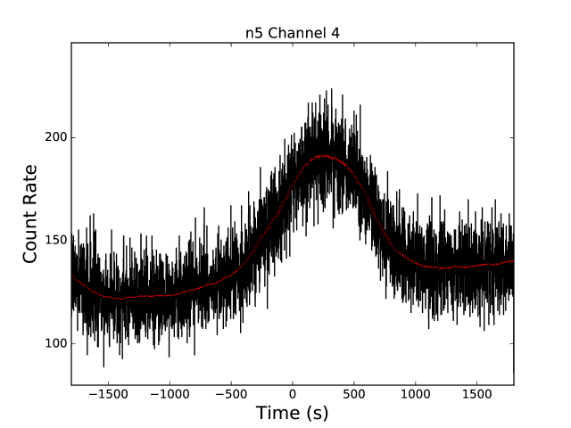
Figure 1: Background estimation of GBM data for a duration of an hour for CTIME channel 4 in NaI detector 5.

Applying this technique specifically to GBM data, the minimum time separation between two detected events allowed by the GBM onboard electronics is $2.6\ \mu$s, therefore any bin width $t$ shorter than this can be used. The actual implementation of this algorithm, for purposes of speed and efficiency, allows the duration of the sliding window to vary by keeping the number of events in the window constant. An additional benefit of allowing a varying window size is that the background can be properly estimated as the background rapidly (but smoothly) increases and decreases during periods of high particle activity and during entrance to/exit from the South Atlantic Anomaly (SAA). Testing with several days of GBM data, an appropriate initial sliding window duration of $\sim$125 s for the average GBM background has been chosen. Within the sliding window, Equation 2 is calculated and estimated as the background rate at the center of the window, thereby allowing the background rate to be estimated at the time of each individual TTE event. In practice, this is likely overkill, and the rate can be down-sampled or interpolated to a regular interval. An example of this background estimation is shown in Figure 1 for an hour of data. Because the rate estimate is applied to the center of the window, the first half of the initial window and the second half of the final window will not have a background estimate. We can, however, allow the sliding window duration to truncate at the beginning and end of these windows, which produces rate estimates with representatively larger uncertainties. This method is particularly applicable when Fermi enters and exits the SAA. The variance in the background rate estimate is simply $\lambda/T$. We calculate this uncertainty and include it in the likelihood calculation described in LB15.

4 Template Spectra

The LB15 search used a set of three template photon spectra, which are folded through each of the GBM detector responses and compared to the observed count spectra of a time of interest. These spectra were the same three that are used in the GBM localization algorithms for GRBs produced by the GBM team (see Connaughton et al., 2015, for details), which has localized $>$1900 GRBs. The spectra are all Band functions (Band et al., 1993), which is a smoothly-broken power law defined by low- and high-energy power-law indices, and the peak of the $\nu F_{\nu}$ spectrum, $E_{\rm peak}$. The three template spectra are typically referred to as ‘Soft,’ ‘Normal,’ and ‘Hard’ since the parameters were chosen to roughly and broadly sample the full spectral diversity of GRBs in the GBM energy band, from spectrally softer long GRBs to harder short GRBs. In practice, the ‘Soft’ spectrum is also used to localize SGR outbursts (van der Horst et al., 2010) and other soft Galactic sources (e.g. Jenke et al., 2016), of which many are present in the GBM data. Although the spectral templates may not individually be a perfect match for any particular GRB (or GRB-like) spectrum, they span the range of observed spectral behavior of GRBs in the GBM band, and they have performed well in discovering particular weak signals in GBM data, as shown by the LB15 search.

While the soft and normal spectra are typically good matches for long GRBs, the hard spectrum has a very shallow (and unphysical) high-energy power-law index of -1.5. Of more concern, however, is that very few GBM-triggered short GRBs are actually best fit by a Band function. Instead, most detected short GRBs have a spectrum that is best-modeled as a power-law with an exponential high-energy cutoff:

$$f(E)=A\ \biggl{(}\frac{E}{E_{\rm piv}}\biggr{)}^{\alpha}\exp\biggl{[}-\frac{(\alpha+2)\ E}{E_{\rm peak}}\biggr{]}.$$ (3)

The maximum of the joint distribution for the cutoff power law for observed short GRBs is index, $E_{\rm peak}$ = $\sim$ (-0.4, 600 keV), however some of the softer GRBs are adequately matched by the normal spectrum, so we choose to create a cutoff power law template with index, $E_{\rm peak}$ = (-0.5, 1.5 MeV) which should better match the averaged spectrum of hard short GRBs. We have chosen to replace the hard template used in LB15 with this new Comptonized template for O2.

5 Candidate Filters

The LB15 search was formulated and optimized to find weak short GRB-like events in the GBM data. GBM data can be very complex and filled with many persistent and transient sources from all over the sky (and Earth), therefore it should be of no surprise that there exists phenomena uninteresting to the search that are nevertheless ‘discovered’ by the search. These phenomena contribute to the false alarm rate (FAR), which is an empirical distribution based on what the search finds. The FAR estimation does not require perfect statistical technique, nor does it require efficiency in the search algorithm, however the FAR will be empirically lower for a statistically sound and efficient search compared to an inefficient search. Specifically, efficient identification and rejection of signals that are obviously unrelated to GW sources will reduce the empirical FAR and thereby improve the significance of a true gamma-ray signal detected in conjunction with a GW signal.

The LB15 search employed during the LIGO O1 run included a filter that removed single-detector phosphorescence events (Fishman & Austin, 1977) from contaminating the FAR. The FAR estimate over the two months of LIGO S6 run and for 2.7 days around the GW150914-GBM candidate included only this filter. Inspection of some of the more significant false alarms found that they were caused by areas of poor background estimation, approach and exit from the SAA, solar flare events, and Galactic sources, and therefore we would like to filter out these types of false alarm events.

5.1 Removing Bad Background

We wish to filter out events due to bad background estimation. In particular, the background estimation described in Section 2 can be biased by strong or very long sources in the data, as well as occultation steps in the lower energy channels when a bright persistent source rises or sets behind the Earth limb. To determine if the background estimate is a poor representation of the true background at the time of interest, we consider a ‘dead’ period of 10 s on either side of the time of interest. Beyond this ‘dead’ period, we compare $\sim$50 s of estimated background rate to the same duration of data, binned to 1.024 s resolution. The goodness-of-fit can then be estimated by

$$\chi^{2}=\sum_{i=1}^{N}\frac{(C_{i}-B_{i})^{2}}{C_{i}+\sigma_{B,i}^{2}},$$ (4)

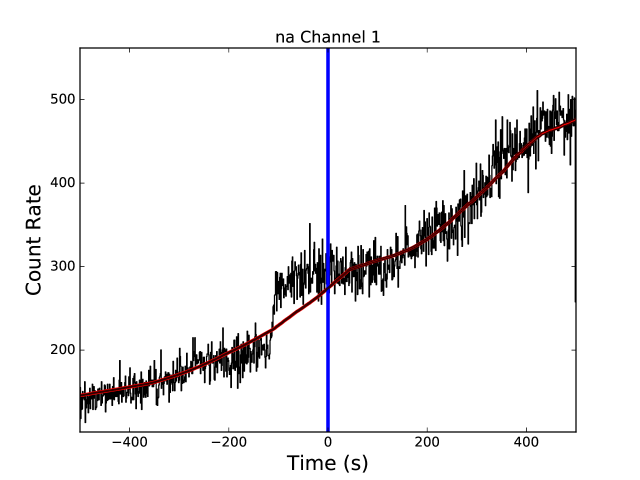
Figure 2: Background estimation during a long, soft source at $\sim$100 s before the time of interest for CTIME channel 1 in NaI detector 10 (also known as ‘NaI a’). The background estimate at the time of interest was flagged as bad due to the poor reduced chi-square statistic in the period prior to the candidate time.

where $C_{i}$ is the number of observed counts in the $i$th bin and $B_{i}$ is the estimated background counts. Dividing $\chi^{2}$ by the number of bins, $N$, gives the reduced chi-squared statistic. Testing on data with known strong sources and occultation steps, a reasonable threshold to flag the background as problematic is $\chi^{2}/N=1.8$. Very few false positive background errors are flagged with this threshold. Figure 2 shows an example where this method identifies a bias of the background estimation due to a nearby soft source.

The LB15 search is designed such that individual channels for individual detectors can be discarded if deemed necessary. In the case of a poor background fit to one or two channels for a single detector, those channels would be removed from the likelihood calculation, but the rest of the data for that detector could be used. Because both the null and alternate hypotheses in the likelihood ratio calculation use the same data for a time of interest, flagging particular channels for removal from the analysis is statistically valid. The LB15 search, however, employs a likelihood that looks for coherent and consistent signal over the entire GBM energy band in all detectors, therefore if too many energy channels from a detector or multiple detectors are removed, the likelihood of a signal over background will be significantly diminished.

5.2 Removing Sharp SAA Rate Changes

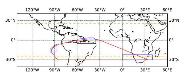
Figure 3: The SAA region where the GBM detectors are disabled is marked in red. The extended SAA regions that we use for event filtering are marked by the blue polygons. The yellow dashed lines show the North-South extent of the Fermi orbit.

Although the background estimation detailed in Section 2 can model the background during approach and exit from the SAA (albeit with larger uncertainty), there may be particular times when the rate increase/decrease is too steep during periods of high particle activity when the true region of the SAA expands or geographically shifts beyond the SAA polygon stored in the Fermi flight software. For this reason, it is desirable to implement an extended SAA polygon and filter out any events that happen when Fermi is within the expanded polygon, which is shown in Figure 3. This filter can be implemented outside of the LB15 search so that if a time of interest is within the expanded polygon (but the GBM detectors are still collecting data), a search can still be performed without the filter at the cost of a higher FAR.

5.3 Likelihood Calculation Pre-Filter

The likelihood ratio calculation, as described in LB15, determines the likelihood that a candidate is a real signal as opposed to a background fluctuation. This calculation requires an estimation of the signal amplitude that maximizes the likelihood of the alternate hypothesis that a signal exists (Eq. 13 of LB15). The signal amplitude solution must be solved numerically as there exists no closed-form analytical solution. The LB15 search performed this numerical optimization using Newton’s method on every single time bin searched. This evaluation is the costliest part of the LB15 search, so we have included a pre-filter to the numerical calculation so that initial guess log-likelihood ratio values of $\leq 5$ are not treated to the full numerical optimization. This value is chosen because it is well below the significance threshold for a candidate signal. We have tested to ensure that the initial guess log-likelihood ratios $\leq 5$ do not become ‘significant’ candidate detections. Implementing this pre-filter has produced up to a factor of $\sim 5$ increase in speed.

6 Joint Spatio-Temporal Ranking Statistic

The LB15 search during O1 used the LogLR as the ranking statistic for significance, specifically Equation 20 in LB15, which a assumes a uniform sky prior. We now choose to include a location prior in the form of a LIGO sky map. For this we use equation 21 from LB15:

$$\Lambda_{GW-GBM}=\int{d\Omega P_{GW}(\Omega)\Lambda_{GBM}(\Omega)},$$ (5)

where $P_{GW}(\Omega)$ is the LIGO localization used as a prior probability distribution on the sky and $\Lambda_{GBM}$ is the GBM likelihood ratio which is also a function of sky position, among other dependencies.

7 Trivial Code Modifications

The code was updated from Python 2 to Python 3, as well as updating the modules and functions to modern versions. An incorrect sign in the reference log-likelihood was corrected (this has no effect on any of the FAR calculations as all log-likelihood ratios were modified by the same constant value). The original version of the code was written to run on LIGO clusters some time ago and, as a result, optimized memory usage. We have removed most of this in favor of speed.

A parallelized version of the polynomial interpolation that numerically calculates the log-likelihood value was implemented using the Theano module (Al-Rfou et al., 2016). This implementation, along with the switch to Python 3, produces identical results to the LB15 search.

8 Validation

We have validated the implemented changes by testing the search on triggered short GRBs, simulated GRBs injected into real GBM data, and on background with no known sources to estimate the change in the FAR.

8.1 Validation with Signals

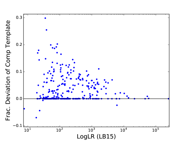
Figure 4: Comparison of the detection statistic when using the original hard Band function template compared to the new Comptonized function template for 310 GBM-triggered short GRBs. The GRBs that lie on the unity line are mostly found with the ‘Normal’ template instead of the hard or Comptonized templates.

Using 310 short GRBs that triggered GBM, we compared the LB15 using the hard spectral template to the replacement template using the hard Comptonized function. The new template increased the ranking statistic in 84% of the cases, and was equivalent for 14% of the cases, with an overall average 4% increase in the statistic value compared to the original. The increase in the statistic is more significant for lower values of the statistic, where we expect un-triggered short GRBs to be uncovered using this search. The comparison is shown in Figure 4.

Additionally, we ran the search on 51 triggered short GRBs with known sky location (i.e. localized by Swift or the Fermi LAT). The search was run using a Gaussian prior on the sky centered at the true location with a 1$\sigma$ radius of 10 degrees. Ideally if the search correctly localizes a truly associated candidate event with a specific sky prior, then the coincident ranking statistic described in Section 6 should be larger than the ranking statistic resulting from a uniform sky prior. In Figure 5 we show the comparisons between the LB15 search and the search using the new Comptonized template for both the offset of the maximum likelihood location from the true location and the coincident ranking statistic. The offset from the true location is improved for 59% of the short GRBs that are found by the hard or Comptonized templates, while the increase in the coincident ranking statistic is more significant for 68% of the GRBs when using the Comptonized template.

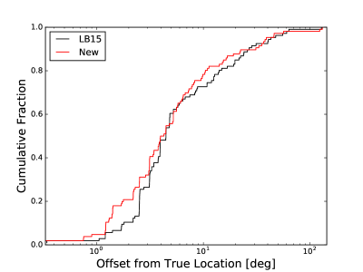
Figure 6: Comparison of the 6 offset of the maximum likelihood location from the true injected location and the 6 coincidence ranking statistic between the LB15 search and the updated search for 105 injected GRBs found by both searches.

Another source test that we have performed is simulating weak short GRBs with a variety of durations, spectra, and locations around the spacecraft and injecting them into real GBM background. By doing this, we can see how often we can detect the injected GRB and accurately localize them. A full estimation of the recovery efficiency as a function of spectrum, location, and duration is ongoing, but we show a sample of tests to compare the LB15 search to the implemented changes. Figure 6 shows the comparison of the true offset from the injected location and the coincidence ranking statistic between the LB15 search and the implemented template and background improvements. In this particular test, 200 GRBs were simulated with varying spectra and locations, and at varying brightness close to the detection threshold. Both searches reasonably recovered 112 of 200 injections, and Figure 6 shows the comparison of the 105 injections that were recovered by both searches. The upgraded search recovered a maximum likelihood location closer to the true injected location 56% of the time compared to a smaller offset 33% of the time for the LB15 search. The increase in the spatial coincidence ranking statistic was greater with the implemented upgrades for 60% of the recovered events and the other 40% were better with the original LB15 search.

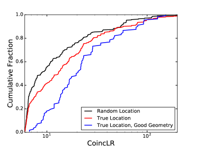
Figure 7: Panel 7 shows the cumulative distributions of the CoincLR ranking statistic for the injected GRB signals at the LIGO sky map locations (red) and injected signals at random locations on the sky (black). The blue distribution shows the CoincLR for the injected GRBs that have a more favorable geometry to the spacecraft compared to the randomly injected sky locations. Panel 7 shows the fractional deviation from the injected CoincLR for a random injection on the sky.

We performed a final test using a set of simulated weak short GRBs injected at times and sky locations consistent with simulated LIGO BAYESTAR localization maps (Singer et al., 2014). The times at which the BAYESTAR maps were simulated were shifted in time such that the LIGO detectors were in the same geometry relative to the simulated originating sky position and during times that GBM had continuous TTE data. We also created a test sample of the simulated short GRBs injected at the same times and with precisely the same spectral shape, but with randomized locations on the sky. We then used the sky maps as priors in the search to determine the effectiveness of providing spatial information to the search in the event that a real signal is detected. Figure 7 shows the comparison of the CoincLR ranking statistic for the two injection sets. The injections consistent with the BAYESTAR maps generally have a larger CoincLR than the random injections, however since the strength of a signal in the GBM data results from a convolution of the photon model with the highly-angular-dependent detector responses, there are cases where the randomly injected location produces a stronger signal in the data than a signal that is consistent with the sky prior. In these cases, the LogLR, the ranking statistic resulting from a uniform sky prior, is also larger than that for the BAYESTAR-consistent injections. Figure 7 demarcates, in blue, the distribution of injected events for which the BAYESTAR-consistent injections have at least comparable signal strength to the randomly injected signals based on LogLR, which is $\sim$67% of the injected signals. All randomized sky injections that have a higher ranking statistic compared to the BAYESTAR-consistent injections are observed at comparatively better geometries to the detectors.

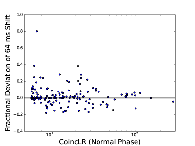
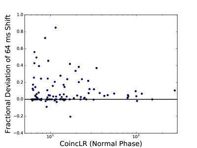
Figure 8: Panel 8 shows the CoincLR ranking statistic of injected signals with the search window centered on the time of interest (Normal Phase), compared to a search window shifted by 64 ms from the time of interest. Panel 8 shows the Normal Phase CoincLR compared to the CoinCLR when utilizing a phase shift factor of 16 for all timescales.

As a final note on the validation of the updated search using injected signals, we investigated the impact of performing the search with a maximum factor 4 phase shift relative to the search timescale as discussed in Section 2, rather than a constant 64 ms phase shift. The targeted search is based on searching a time window centered on a particular time of interest (what we refer to here as Normal Phase), so we re-ran the search on the BAYESTAR-consistent injections but shifted the center of the time window by 64 ms relative to the time of interest. The comparison of the ranking statistic resulting from this shift is shown in Figure 8. Because search timescales $>$ 256 ms are not utilizing the ability to perform a 64 ms phase shift of the binned data, the resulting CoincLR can change by a considerable amount (an average of $\sim$10% here), which can result in a large change in the associated FAR for a particular event. This implies that the current search, as devised for LIGO O2a, requires some amount of “luck” to find a weak, short signal because of this phasing issue. If, on the other hand, we run the search allowing for a maximum phase shift factor of 16 for all timescales, the case improves considerably as shown in Figure 8, where the CoincLR increases in nearly every case, and the overall average change is a $\sim$9% increase in CoincLR over the search using the Normal Phase. Increasing the number of phase shifts for the longer timescales effectively increases the size of the search space, therefore the FAR would have to be recalculated. Because the FAR estimation is very time-consuming (and even more so if the factor 16 phase shift for all timescales were implemented) we leave this potential change for future study and continue with the factor 4 phase shift for LIGO O2a.

8.2 Validation with Background

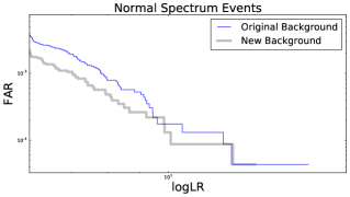
(a) ‘Normal’ Template

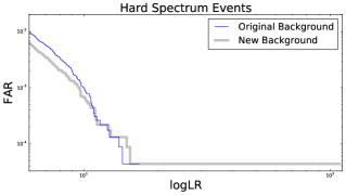
(b) ‘Hard’ Template

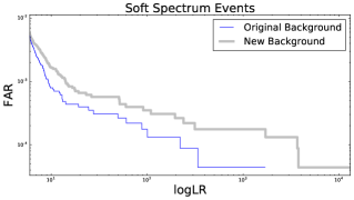
(c) ‘Soft’ Template

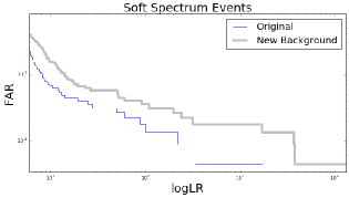
(d) ‘Soft’ Template $>2$ s

Figure 9: The FAR comparison between the LB15 search and the new background estimation described in Section 3 for each of the three original spectral templates used in LB15. Panels 9(a)– 9(c) show the FAR combining all candidate timescales from 0.256 s up to 8.192 s. Panel 9(d) shows the FAR for the soft template only at timescales $>2$ s, indicating that the overrun in the new FAR compared to LB15 is due to longer timescale candidates.

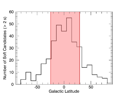
Figure 10: The Galactic latitude distribution of 363 significant soft candidates at $>2$ s timescale using the new background estimation. The red shaded region represents the angular extent of 67% of the candidates. Note that only the maximum likelihood location was considered, and this distribution does not take into account localization uncertainty.

In addition to testing the changes with real GRBs and injected signals, we test over regions of background where candidate signals are not expected (around the times of the BAYESTAR injections in the previous section) to evaluate the new FAR and compare it to the FAR of the LB15 search. Figure 9 shows the FAR comparison using the new background estimation for each of the three templates. For both the ‘Normal’ and the ‘Hard’ templates, the FAR with the new background clearly under-runs the FAR from LB15, thereby making the detection of candidates more significant. The FAR for the ‘Soft’ template clearly over-runs compared to LB15, but as can be seen in Figure 9(d), the cause of the over-run is due to events that are $>2$ s in duration. One possible explanation for this over-run is a more efficient recovery of spectrally soft Galactic sources that may be flaring in the low-energy channels of the GBM data. Indeed, if we map the maximum likelihood localizations of all the events in Figure 9(d), we find that a large fraction of events are consistent with a Galactic origin, shown in Figure 10. This implies that the FAR for the ‘Soft’ template is bounded by the amount of soft Galactic activity GBM observes, and we are currently investigating using a Galactic sky prior to classify soft events that strongly localize to the Galactic Plane as well as dividing the FAR distributions into different timescales. Another class of events that can contribute to the longer duration soft events are solar flares, which are usually easy to distinguish from astrophysical events by inspection of the GBM lightcurves and contemporaneous GOES data.

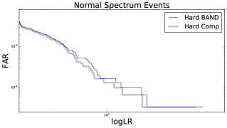
(a) ‘Normal’ Template

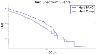
(b) ‘Hard’ Template

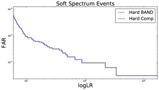
(c) ‘Soft’ Template

Figure 11: The FAR comparison between the LB15 search using the ‘Hard’ Band function template and the new ‘Hard’ Comptonized template described in Section 4. The FAR distribution for the ‘Normal’ template is affected by the change in the ‘Hard’ template as some events are now found with a higher logLR in the ‘Hard’ template. The distribution for the ‘Soft’ template is unaffected.

In Figure 11, we show the additional improvement made to the FAR by replacing the hard template in LB15 with the new Comptonized template. Note that because the templates have some overlap in spectral parameter space, an event may be ‘detected’ in more than one template, however, the search only considers the template with the highest ranking statistic. The result of this can be seen in the difference between the FAR for the ‘Normal’ spectral template when the ‘Hard’ spectral template is replaced with the new Comptonized template: some events that were ‘detected’ with the ‘Normal’ template were shifted over to the ‘Hard’ template. The ‘Soft’ template is left unaffected by this change since it occupies a completely disjoint part of the parameter space relative to the ‘Hard’ template.

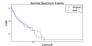
(a) ‘Normal’ Template

(b) ‘Hard’ Template

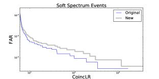
(c) ‘Soft’ Template

Figure 12: The FAR comparison between the LB15 search (blue) and all of the combined updates (gray): new background, new ‘Hard’ template, the spatial CoincLR ranking statistic, and the 64 ms binned data.

Combining all of the aforementioned changes results in the final FAR comparison plots shown in Figure 12. We find an obvious overall improvement in the FAR distribution for the ‘Normal’ and ‘Hard’ spectral templates compared to the LB15 search. The FAR distribution for the ‘Soft’ spectral template does not show the same improvement. This is likely due to the fact that GBM observes a large population of real signals, mostly Galactic, at lower energies, and the new background improves the detection of these events that are longer than 2 s. Until a future improvement is implemented, such as a Galactic sky prior, any event of interest discovered by the ‘Soft’ template will suffer a higher FAR and therefore a lower significance compared to the LB15 search. The impact that the ‘Soft’ template has on detecting a canonical short GRB, however, is minimal since almost all known short GRBs detected by GBM would be detected with the ‘Normal’ or ‘Hard’ template (possibly with the exception of precursors to the prompt emission). Note that the use of the 64 ms binned data now allows more phase shifts for the 256 ms and 512 ms timescales (up to a factor of four), thereby increasing the effective number bins searched. This results in an overall higher FAR, however, the improvements from using the new background, the new ‘Hard’ template, and the new ranking statistic more than offset this increase in the FAR.

9 Case Study: GW150914-GBM

Although the updates to the LB15 search were not specifically motivated by the detection of a short, hard transient candidate $\sim$0.4 s after LIGO triggered on GW150914, the presence of such a candidate allows us to compare how the updated search fares relative to the LB15 search that found the candidate. Figure 13 shows this comparison with the ranking statistic of the candidate marked on both FAR distributions. The FAR distribution using the LB15 search covers the same time as the FAR distribution using the O2a search for a fair comparison and is therefore slightly different than the distribution found in Connaughton et al. (2016).

The LB15 search found that the most significant signal was in the 1.024 s timescale, and because the CTIME datatype is natively binned at 256 ms resolution, this allows a phase shift factor of 4 for the 1.024 s timescale. The search using the TTE data binned at 64 ms allows a phase shift factor of 4 for the 256 ms timescale, however we have maintained the LB15 maximum phase shift factor of 4 for any single timescale, which means that we still only perform a factor 4 phase shift for the 1.024 s timescale, as described in Section 2. This implies that the O2a search will not necessarily use the same binning phase used in the O1 search. In fact, Figure 13 shows the result of maintaining the factor 4 phase shift for the 1.024 s timescale by offsetting the search window by 64 ms, four times. The ranking statistic varies from 8.2–12.9 (the largest value corresponding to the phase closest to the O1 search phase), which results in a pre-trials FAR ranging from $1.7\times 10^{-3}$–$3.9\times 10^{-5}$ Hz (the O1 pre-trials FAR was $1.2\times 10^{-4}$ Hz). The maximum relative change in the ranking statistic for the 64 ms phase shifts is 36%, consistent with what was found in Section 8.1.

Figure 5: Comparison of the 5 offset of the maximum likelihood location from the true location and the 5 coincidence ranking statistic between the LB15 search templates and the new Comptonized template for 51 triggered short GRBs with known location.

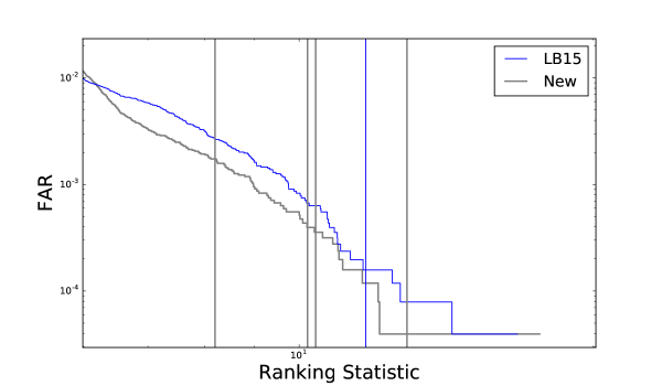
Figure 13: The comparison of the 150914-GBM candidate as detected by the LB15 search and the combined improvements for O2a. The blue line marks the LB15 ranking statistic value relative to FAR for the LB15 search, and the four gray lines mark the O2a ranking statistic relative to the O2a FAR for the Normal Phase and three 64 ms offsets relative to the LIGO detection time.

References

- Abbott et al. (2016) Abbott, B. P., et al. 2016, Phys. Rev. Lett., 116, 061102
- Al-Rfou et al. (2016) Al-Rfou, R., Alain, G., Almahairi A., et al. 2016, arXiv:1605.02688
- Band et al. (1993) Band, D., Matteson, J., Ford, L., et al. 1993, ApJ, 43, 281
- Blackburn et al. (2015) Blackburn, L., Briggs, M. S., Camp, J., et al. 2015, ApJS, 217, 8
- Connaughton et al. (2015) Connaughton, V. C., Briggs, M. S., Goldstein, A., et al. 2015, ApJS, 216, 32
- Connaughton et al. (2016) Connaughton, V. C., Burns, E., Goldstein, A., et al. 2016, ApJ, 826, L6
- Fishman & Austin (1977) Fishman, G. J. & Austin, R. W. 1997, Nucl. Instrum. Methods, 140, 193
- van der Horst et al. (2010) van der Horst, A. J., Connaughton, V. C., Kouveliotou, C., et al. 2010, ApJ, 711, L1
- Jenke et al. (2016) Jenke, P. A., Wilson-Hodge, C. A., Homan, J. et al. 2016, ApJ, 826, 37
- Meegan et al. (2009) Meegan, C., Lichti, G., Bhat, N., et al. 2009, ApJ, 702, 791
- Racusin et al. (2016) Racusin, J., Burns, E., Goldstein, A., et al. 2016, arXiv:1606.04901
- Singer et al. (2014) Singer, L. P., Price, L. R., Farr, B., et al. 2014, ApJ, 795, 105
- Singer et al. (2015) Singer, L. P., Kasliwal, M. M., Cenko, B. S., et al. 2015, ApJ, 806, 52