Quantum phases of interacting three-component fermions
under the influence of spin-orbit coupling and Zeeman fields

Abstract

We describe the quantum phases of interacting three component fermions in the presence of spin-orbit coupling, as well as linear and quadratic Zeeman fields. We classify the emerging superfluid phases in terms of the loci of zeros of their quasi-particle excitation spectrum in momentum space, and we identify several Lifshitz-type topological transitions. In the particular case of vanishing quadratic Zeeman field, a quintuple point exists where four gapless superfluid phases with surface and line nodes converge into a fully gapped superfluid phase. Lastly, we also show that the simultaneous presence of spin-orbit and Zeeman fields transforms a momentum-independent scalar order parameter into an explicitly momentum-dependent tensor in the generalized helicity basis.

The effects of spin-orbit coupling are ubiquitous in the physical world ranging from planetary motion in the macroscopic scale to the hyperfine structure of atoms in the microscopic universe. At the quantum level, spin-orbit coupling is a relativistic manifestation associated with the motion of electrons around the atomic nucleus landau-1980 . In electronic solids, this has lead to non-trivial effects such as the emergence of topological insulators and superconductors hasan-2010 ; zhang-2011a , as well as non-centrosymmetric superconductivity sigrist-2009 . However, neither spin-orbit coupling nor interactions can be changed substantially for a given condensed matter system.

Recently, artificial spin-orbit coupling with adjustable strength were created in neutral ultra-cold atoms. This was first achieved in the context of bosonic atoms, such as ⁸⁷Rb, by using a set of Raman beams to transfer momentum to the center of mass of atoms depending on their internal hyperfine state spielman-2011 . The same technique was also used for fermionic atoms, such as ⁴⁰K, which have the added advantage of the tunability of interactions via Fano-Feshbach resonances spielman-2013 ; jiang-2014 ; chapman-2011 . For ⁸⁷Rb, the interactions can not be adjusted, but it has been possible to study experimentally spielman-2011 and theoretically wu-2011 ; ho-2011 ; stringari-2012 the emergence of superfluid phases in the presence of simultaneous artificial spin-orbit coupling and Zeeman fields for systems of two hyperfine states. For ⁴⁰K, heating from the Raman beams made it difficult to cool down these fermions to sufficiently low temperatures spielman-2013 ; jiang-2014 . This has precluded the probing of superfluid phases that have been predicted theoretically shenoy-2011 ; zhang-2011b ; zhai-2011 ; pu-2011 ; han-2012 ; seo-2012 for two hyperfine states, when the interactions are changed. Although, presently, finite temperature theories for spin-orbit coupled fermions with two hyperfine states have been developed only for two-dimensional systems devreese-2014 , it has not yet been possible to reduce the temperature of the atomic gas and reach the superfluid regime in the presence of Raman beams. This has been true even for the intermediate or strongly attractive regimes, where the critical temperature for superfluidity is a fraction of the Fermi energy.

Currently, a new experimental method is being developed where artificial spin-orbit coupling and Zeeman fields can be created by a specially designed chip. In this case, spatially modulated radio-frequency fields can be created and can couple directly to atoms in a nearby cloud goldman-2010 . This procedure can avoid the deleterious thermal effects caused by Raman beams, and may allow for the exploration of superfluid phases of fermionic systems with two or more hyperfine states. In anticipation of the use of this technique, we propose the exploration of fermionic systems with three internal (or hyperfine) states in the presence of spin-orbit and Zeeman fields, where novel superfluid phases emerge as discussed below.

To describe interacting three-component fermions under the influence of spin-orbit and Zeeman fields, we start with the most general independent-particle Hamiltonian that could result from a suitably designed radio-frequency chip or Raman beams in the rotating frame kurkcuoglu-2015

$${\bf H}_{0}({\bf k})=\left(\begin{array}[]{ccc}\varepsilon_{1}({\bf k})&\Omega_{12}&\Omega_{13}\\ \Omega_{12}^{*}&\varepsilon_{2}({\bf k})&\Omega_{23}\\ \Omega_{13}^{*}&\Omega_{23}^{*}&\varepsilon_{3}({\bf k})\\ \end{array}\right),$$ (4)

where $\varepsilon_{s}({\bf k})=({\bf k}-{\bf k}_{s})^{2}/(2m)+\eta_{s}$ represents the energy of internal state $s=\{1,2,3\}$ after net momentum transfer ${\bf k}_{s}$, and $\eta_{s}$ is a reference energy of the atom at internal state $s$. The matrix elements $\Omega_{ss^{\prime}}$ represent Rabi frequencies between atomic states $s$ and $s^{\prime}$.

In this manuscript, instead of pursuing the most general theoretical case shown in Eq. (4), we consider a simpler experimental setup, where the Rabi frequency $\Omega_{13}=0$, indicating that there is no coupling between states $1$ and $3$. In addition, we consider that the Rabi frequencies associated with the transitions from states $1$ to $2$ and from $2$ to $3$ to real and equal, that is, $\Omega_{12}=\Omega_{12}^{*}=\Omega_{23}=\Omega_{23}^{*}=\Omega$. Furthermore, we choose a symmetric situation, where momentum transfers occur only to state 1 and 3, such that ${\bf k}_{1}=k_{T}{\hat{\bf x}}$, ${\bf k}_{2}=0$, and ${\bf k}_{3}=-k_{T}{\hat{\bf x}}$, where $k_{T}$ is the magnitude of the momentum transferred to the atom by the photons. Lastly, we can define an energy reference via the sum $\sum_{s}\eta_{s}=\eta,$ leading to internal energies $\eta_{1}=-\delta,$ $\eta_{2}=\eta$ and $\eta_{3}=+\delta,$ where $\delta$ represents the detuning.

A simple rearrangment of the chip-atom or light-atom interaction Hamiltonian matrix allows us to write it in a more compact and transparent notation as

$${\bf H}_{0}({\bf k})=\varepsilon({\bf k}){\bf 1}-h_{x}({\bf k}){\bf J}_{x}-h_{z}({\bf k}){\bf J}_{z}+b_{z}{\bf J}_{z}^{2},$$ (5)

where ${\bf J}_{\ell}$, with $\ell=\{x,y,x\}$, are spin-one angular momentum matrices. Here, $\varepsilon({\bf k})={\bf k}^{2}/(2m)+\eta$ is a reference kinetic energy which is the same for all internal states, $h_{x}({\bf k})=-\sqrt{2}\Omega$ is the spin-flip (Rabi) field, and $h_{z}({\bf k})=2k_{T}k_{x}/(2m)+\delta$ is a momentum dependent Zeeman field along $z$-axis, which is transverse to the momentum transfer direction ($x$-axis), and $b_{z}=k_{T}^{2}/(2m)-\eta$ is the quadratic Zeeman term. Notice that $h_{z}({\bf k})$ contains the spin-orbit coupling term $2k_{T}k_{x}/(2m)$ as well as the detuning $\delta$. Very recently, a similar Hamiltonian was created experimentally for spin-one bosonic ⁸⁷Rb atoms spielman-2015 and magnetic phases of this system were investigated.

The chip-atom (or light-atom) interaction Hamiltonian can be written in second-quantized notation as

$${H}_{{\rm CA}}=\sum_{\bf k}{\bf\Psi}^{\dagger}_{\bf k}{\bf H}_{0}({\bf k}){\bf\Psi}_{\bf k}$$ (6)

where the spinor operator is ${\bf\Psi}^{\dagger}_{\bf k}=(\psi_{1}^{\dagger}({\bf k}),\psi_{2}^{\dagger}({\bf k}),\psi_{3}^{\dagger}({\bf k}))$, with $\psi_{s}^{\dagger}({\bf k})$ creating a fermion with momentum ${\bf k}-{\bf k}_{s}$ in internal state $s$. The Hamiltonian $H_{\rm CA}$ can be diagonalized via the rotation ${\bf\Phi}({\bf k})={\bf U}({\bf k}){\bf\Psi}({\bf k}),$ which connects the three-component spinor ${\bf\Psi}({\bf k})$ in the original spin basis to the three-component spinor ${\bf\Phi}({\bf k})$ representing the basis of eigenstates. The matrix ${\bf U}({\bf k})$ is unitary and satisfies the relation ${\bf U}^{\dagger}({\bf k}){\bf U}({\bf k})={\bf 1}$. The diagonalized Hamiltonian matrix is ${\bf H}_{D}({\bf k})={\bf U}({\bf k}){\bf H}_{0}({\bf k}){\bf U}^{\dagger}({\bf k})$ with matrix elements ${\bf H}_{D,\alpha\beta}({\bf k})={\mathcal{E}}_{\alpha}({\bf k})\delta_{\alpha\beta},$ where $\mathcal{E}_{\alpha}({\bf k})$ are the eigenvalues of ${\bf H}_{0}({\bf k})$ discussed above. The three-component spinor in the generalized helicity eigenbasis is ${\bf\Phi}^{\dagger}({\bf k})=\left[\phi^{\dagger}_{\Uparrow}({\bf k}),\phi^{\dagger}_{0}({\bf k}),\phi^{\dagger}_{\Downarrow}({\bf k})\right],$ where $\phi^{\dagger}_{\alpha}({\bf k})$ is the creation operator of a fermion with eigenenergy $\mathcal{E}_{\alpha}({\bf k})$ with generalized spin label $\alpha$. The unitary matrix

$${\bf U}({\bf k})=\left(\begin{array}[]{c c c}u_{\Uparrow 1}({\bf k})&u_{\Uparrow 2}({\bf k})&u_{\Uparrow 3}({\bf k})\\ u_{01}({\bf k})&u_{02}({\bf k})&u_{03}({\bf k})\\ u_{\Downarrow 1}({\bf k})&u_{\Downarrow 2}({\bf k})&u_{\Downarrow 3}({\bf k})\end{array}\right)$$ (10)

has rows that satisfy the normalization condition $\sum_{s}|u_{\alpha s}({\bf k})|^{2}=1,$ where $\alpha=\{\Uparrow,0,\Downarrow\}$.

We use as units the Fermi energy $E_{F}=k_{F}^{2}/(2m)$ and the Fermi momentum $k_{F}=(2\pi^{2}n)^{1/3},$ based on the total density of fermions $n=3k_{F}^{3}/(6\pi^{2})$ with initial identical kinetic energies $\epsilon_{\bf k}={\bf k}^{2}/(2m)$ for all three internal states. This means that our reference system is that with all parameters $\eta,k_{T},\Omega$ and $\delta$ set to zero.

In Fig. 1, we show plots of eigenvalues $\mathcal{E}_{\alpha}({\bf k})$ versus momentum $k_{x}$ for fixed momentum transfer $k_{T}=0.35k_{F}$ and zero detuning $\delta=0$. The figures at left, middle, right represent, respectively, the cases of quadratic Zeeman shift $b_{z}=-E_{F},0,+E_{F}$. The top panels correspond to $\Omega=0$, and the bottom panels to $\Omega=E_{F}$. In the top panels, notice that double minima are present in $\mathcal{E}_{\Uparrow}({\bf k})$ when $b_{z}<0$ and $b_{z}=0$ and that double minima appear in $\mathcal{E}_{0}({\bf k})$, when $b_{z}>0$. This occurs only for small $\Omega/E_{F}$. In the bottom panels, notice that double minima in all dispersions disapappear, because the Rabi frequency $\Omega=E_{F}$ is sufficiently large.

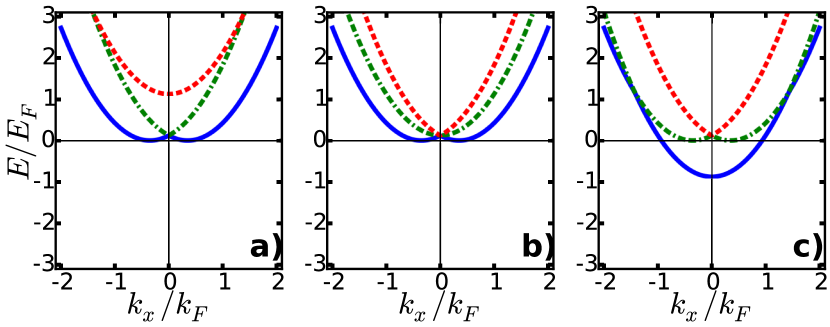
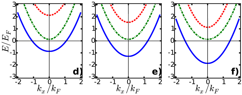
Figure 1: (color online) Eigenvalues $\mathcal{E}_{\alpha}({\bf k})$ versus $k_{x}$ in qualitatively different situations corresponding to momentum transfer $k_{T}=0.35k_{F}$, and quadratic Zeeman shift $b_{z}=-E_{F}$ (left); $b_{z}=0$ (middle); $b_{z}=E_{F}$ (right). The top (bottom) panels correspond to Rabi frequency $\Omega=0$ $(\Omega=E_{F})$. The solid blue line corresponds to $\mathcal{E}_{\Uparrow}({\bf k})$, the dot-dashed-green line to $\mathcal{E}_{0}({\bf k})$ and the dashed-red line to $\mathcal{E}_{\Downarrow}({\bf k})$, aslo at $T=0.02E_{F}$.

In order to study the quantum phases of three-component fermions, we add interactions between atoms in different internal states and consider contact attractive interactions $-g_{ss^{\prime}}\delta({\bf r}-{\bf r}^{\prime})$ of strength $g_{ss^{\prime}}>0$, between internal states $s\neq s^{\prime}$ only. Notice that $g_{ss^{\prime}}$ has dimensions of energy times volume. The atom-atom interaction Hamiltonian can be written in momentum space as

$$H_{{\rm AA}}=-\frac{1}{V}\sum\limits_{{\bf Q},\left\{s\neq s^{\prime}\right\}}g_{ss^{\prime}}b_{ss^{\prime}}^{\dagger}({\bf Q})b_{ss^{\prime}}({\bf Q}),$$ (11)

where $V$ is the volume, ${\bf Q}$ is the center-of-mass momentum of fermion pairs characterized by the operator $b_{ss^{\prime}}^{\dagger}({\bf Q})=\sum_{\bf k}\psi_{s}^{\dagger}({\bf k}+{\bf Q}/2)\psi_{s^{\prime}}^{\dagger}(-{\bf k}-{\bf Q}/2).$ Thus, the Hamiltonian describing the effects of spin-orbit coupling, Zeeman fields and atom-atom interactions is

$$H=H_{{\rm CA}}+H_{{\rm AA}}-\mu{\hat{N}},$$ (12)

where ${\hat{N}}=\sum_{s,{\bf k}}\psi_{s}^{\dagger}({\bf k})\psi_{s}({\bf k})$ represents the total number of particles. We are interested in uniform superfluid phases, so we focus on the case of pairing at zero center-of-mass momentum only, that is, ${\bf Q}=0$.

We define the order parameter for superfluidity as the expectation value $\Delta_{ss^{\prime}}=-g_{ss^{\prime}}\langle b_{ss^{\prime}}({\bf 0})\rangle/V,$ and write the reduced mean-field Hamiltonian as

$$H_{\rm MF}=\frac{1}{2}\sum_{\bf k}{\bf\Psi}^{\dagger}_{N}({\bf k}){\bf H}_{\rm MF}({\bf k}){\bf\Psi}_{N}({\bf k})+V\sum_{s\neq s^{\prime}}\frac{|\Delta_{ss^{\prime}}|^{2}}{g_{ss^{\prime}}}+{\mathcal{C}}(\mu)$$ (13)

where the six-component Nambu spinor is ${\bf\Psi}^{\dagger}_{N}({\bf k})=\left[\Psi_{1}^{\dagger}({\bf k}),\Psi_{2}^{\dagger}({\bf k}),\Psi_{3}^{\dagger}({\bf k}),\Psi_{1}({-\bf k}),\Psi_{2}({-\bf k}),\Psi_{3}({-\bf k})\right]$ and the function ${\mathcal{C}}(\mu)=\frac{1}{2}\sum_{{\bf k}s}\xi_{s}(-{\bf k})$ contains the term $\xi_{s}({\bf k})=\varepsilon_{s}({\bf k})-\mu$ representing the residual kinetic energy contributions. Here, $\varepsilon_{s}({\bf k})$ represents the diagonal matrix elements of ${\bf H}_{0}({\bf k})$ given by $\varepsilon_{1}({\bf k})=\varepsilon({\bf k})-h_{z}({\bf k})+b_{z};$ $\varepsilon_{2}({\bf k})=\varepsilon({\bf k});$ and $\varepsilon_{3}({\bf k})=\varepsilon({\bf k})+h_{z}({\bf k})+b_{z}.$

The $6\times 6$ mean-field Hamiltonian matrix is

$${\bf H}_{\rm MF}({\bf k})=\left(\begin{array}[]{cc}\overline{\bf H}_{0}({\bf k})&{\bf\Lambda}\\ {\bf\Lambda}^{\dagger}&-\overline{\bf H}_{0}^{*}(-{\bf k})\end{array}\right),$$ (16)

where the diagonal block matrix $\overline{\bf H}_{0}({\bf k})={\bf H}_{0}({\bf k})-\mu{\bf 1}$ and the off-diagonal block matrix

$${\bf\Lambda}=\left(\begin{array}[]{ccc}0&\Delta_{12}&\Delta_{13}\\ -\Delta_{12}&0&\Delta_{23}\\ -\Delta_{13}&-\Delta_{23}&0\end{array}\right)$$ (20)

represents the order parameter tensor. In this work, we consider the simpler case where $g_{12}=g_{23}=0$, and $g_{13}=g$, which leads to $\Delta_{12}=\Delta_{23}=0$, and $\Delta_{13}=\Delta$, such that the order parameter tensor $\Delta_{ss^{\prime}}$ is characterized by a single complex scalar $\Delta$.

The quasi-particle and quasi-hole excitation spectrum can be found from the mean-field Hamiltonian in Eq. (16) leading to six energy eigenvalues, which we order as $E_{1}({\bf k})>E_{2}({\bf k})>E_{3}({\bf k})>E_{4}({\bf k})>E_{5}({\bf k})>E_{6}({\bf k}).$ These eigenvalues exhibit quasi-particle/quasi-hole symmetry in momentum space for any value of detuning $\delta$ and Rabi frequency $\Omega$, which means $E_{6}({\bf k})=-E_{1}(-{\bf k}),$ $E_{5}({\bf k})=-E_{2}(-{\bf k})$ and $E_{4}({\bf k})=-E_{3}(-{\bf k}).$ However, each eigenergy $E_{j}({\bf k})$ has well defined parity only when $\delta=0$, in which case $E_{j}({\bf k})=E_{j}({\bf-k})$ has even parity.

To analyze the excitation spectrum $E_{j}({\bf k})$, we need to determine self-consistently the values of the order parameter amplitude $\Delta_{13}=\Delta$ and the chemical potential $\mu$. For this purpose, we write the thermodynamic potential $\mathcal{Q}=-T\ln\mathcal{Z},$ where $\mathcal{Z}=\int\Pi_{s}D\left[\psi^{\dagger}_{s}({\bf k}),\psi_{s}({\bf k})\right]\exp\left[-S\right]$ is the grand-canonical partition function written in terms of the action $S$. At the mean-field level the action is

$$TS_{\rm MF}=-\frac{1}{2}\sum_{n,{\bf k}}{\bf\Psi}_{N}^{\dagger}({\bf k}){\bf G}^{-1}{\bf\Psi}_{N}({\bf k})+V\frac{|\Delta_{13}|^{2}}{g_{13}}+{\mathcal{C}}(\mu),$$

where ${\bf G}^{-1}(i\omega_{n},{\bf k})=\left[i\omega_{n}{\bf 1}-{\bf H}_{\rm MF}({\bf k})\right]$ is the inverse of the resolvent (Green) matrix ${\bf G}(i\omega_{n},{\bf k})$. Here, $\omega_{n}=(2n+1)\pi T$ is the fermionic Matsubara frequency, and $T$ is the temperature. Integration over the fermionic fields leads to the thermodynamic potential

$${\mathcal{Q}}_{\rm MF}=-\frac{T}{2}\sum_{{\bf k}j}\ln\left\{1+\exp\left[-E_{j}({\bf k})/T\right]\right\}+V\frac{|\Delta_{13}|^{2}}{g_{13}}+{\mathcal{C}}(\mu),$$ (21)

where the sum over $j$ includes both quasi-particle and quasi-hole energies $(j=\{1,2,3,4,5,6\})$.

The minimization of ${\mathcal{Q}}_{\rm MF}$ with respect to $\Delta_{13}^{*}$ using the relation $\delta{\mathcal{Q}}_{\rm MF}/\delta\Delta_{13}^{*}=0$ leads to the order parameter equation

$$\frac{V}{g_{13}}\Delta_{13}=\frac{1}{2}\sum\limits_{\bf k}\sum\limits_{j=1}^{3}\tanh\left(\frac{\beta E_{j}({\bf k})}{2}\right)\frac{\partial E_{j}({\bf k})}{\partial\Delta_{13}^{*}},$$ (22)

while fixing the total number of particles for $\Omega\neq 0$ is possible via the thermodynamic relation $N=-\partial{\mathcal{Q}}_{\rm MF}/\partial\mu|_{T,V}$ leading to the number equation

$$N=\frac{1}{2}\sum\limits_{\bf k}\left[\sum\limits_{j=1}^{3}\tanh\left(\frac{\beta E_{j}({\bf k})}{2}\right)\frac{\partial E_{j}({\bf k})}{\partial\mu}+3\right].$$ (23)

Here, the summation over $j$ involves only quasi-particle energies $(j=\{1,2,3\})$, that is, only the positive eigenvalues of the Hamiltonian matrix ${\bf H}_{\rm MF}({\bf k})$, because we used quasi-particle/quasi-hole symmetry to eliminate the quasi-hole energies. Lastly, by using the relation $V/g_{13}=-mV/(4\pi a_{s})+\sum_{\bf k}1/(2\epsilon_{\bf k}),$ we express the bare coupling constant $g_{13}$ in terms of the scattering length $a_{s}$ in the absence of the spin-orbit and Zeeman fields.

Among the quasi-particle excitation energies $E_{1}({\bf k}),$ $E_{2}({\bf k}),$ and $E_{3}({\bf k}),$ only $E_{3}({\bf k})$ may have zeros. In momentum space, the zeros of $E_{3}({\bf k})$ define the loci (points, lines or surfaces) where there is no energy cost to create quasi-particle excitations. Such points, lines or surfaces of zero energy can be used to classify the topologically distinct superfluid phases of three-component fermions.

In Fig. 2, we plot the momentum space loci of $E_{3}({\bf k})=0$ versus $(k_{x},k_{\perp})$, where $k_{\perp}$ represents a radial vector in the $k_{y}k_{z}$ plane, for the case of zero detuning $(\delta=0)$. We show only the first quadrant, because the loci have polar symmetry in the $k_{y}k_{z}$ plane, and reflection symmetry in the $k_{x}$ direction. This means that points along the $k_{\perp}$ axis represent circles in the $k_{y}k_{z}$ plane, and that lines in the $k_{x}k_{\perp}$ represent surfaces in three-dimensional momentum space $(k_{x},k_{y},k_{z})$. The top panels show the momentum space loci for normal phases $N1,N2,N3$, represent one, two or three distinct surfaces, respectively. These are the Fermi surfaces associated with the normal phases. In the bottom panels, we show the nodal structure of three superfluid phases that have a boundary with the normal state, when the quadratic Zeeman term is zero $(b_{z}=0)$. The phase $R1S0$ has one ring and zero surface of nodes, the phase $R1S1$ has one ring and one surface of nodes, and the phase $R2S1$ has two rings and one surface of nodes. For $b_{z}=0$, there is also a phase with zero rings and one surface of nodes $(R0S1)$, not shown in Fig. 2.

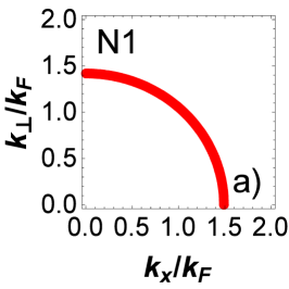
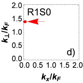
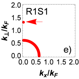
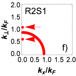
Figure 2: Plots of loci of zero quasi-particle energy $E_{3}(k_{x},k_{\perp})$ in the $k_{x}k_{\perp}$ plane at $T=0.02E_{F}$ for various phases with $b_{z}=0$, where $k_{\perp}$ is the radial component representing $(k_{y},k_{z})$. The phases are: a) $N1$ with $\Omega=1.75E_{F}$ and $1/(k_{F}a_{s})=-1.00$, b) $N2$ with $\Omega=E_{F}$ and $1/(k_{F}a_{s})=-1.00$, c) $N3$ with $\Omega=0.40E_{F}$ and $1/(k_{F}a_{s})=-1.00$, d) $R1S0$ with $\Omega=1.75E_{F}$ and $1/(k_{F}a_{s})=0.80$, e) $R1S1$ with $\Omega=E_{F}$ and $1/(k_{F}a_{s})=0.20$, f) $R2S1$ with $\Omega=0.40E_{F}$ and $1/(k_{F}a_{s})=-0.30$.

In Fig. 3, we plot phase diagrams of Rabi frequency $\Omega/E_{F}$ versus scattering parameter $1/(k_{F}a_{s})$ for quadratic Zeeman shifts $b_{z}=\{0,\pm E_{F}\}$ with spin-orbit coupling parameter $k_{T}=0.35k_{F}$. In Fig. 3b, for $b_{z}=0$, we show the component $\Delta_{\Uparrow\Uparrow}({\bf k})$ of the order parameter tensor in the generalized helicity basis to reveal its odd symmetry and its amplitude for large momentum $k_{x}$. Normal phases $N1$, $N2$ and $N3$ are indicated by dark-gray, light-gray and white colors, respectively. Superfluid phases are color coded: $R1S0$ (red), $R1S1$ (blue), $R2S1$ (green), $R0S1$ (purple), and the fully gapped $(FG)$ phase (yellow). The phase transitions from normal to superfluid are all continuous (second-order), and the transitions between superfluid phases are topological and of the Lifshitz-type lifshitz-1960 . For $b_{z}=0$ (Fig. 3a), there is a quintuple and pentacritical point, where the phases $R1S0$, $R1S1$, $R1S2$, and $R0S1$ converge into a fully gapped phase when rings and surfaces of nodes in momentum space disappear through zero momentum $({\bf k}=0)$. When $\Omega\to 0$, the number of particles in each band is conserved separatelly and spin-orbit coupling can be gauged away, leading to an inert band 2 and to standard crossover phenomena in the superfluid phase for bands 1 and 3.

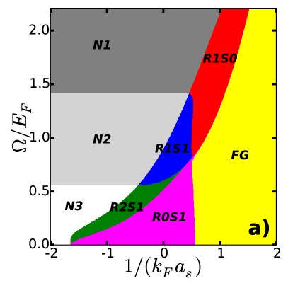
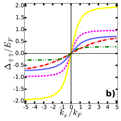
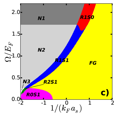
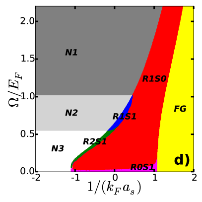
Figure 3: (Color online) Phase diagrams of $\Omega/E_{F}$ versus $1/(k_{F}a_{s})$ for $T=0.02E_{F}$ and $k_{T}=0.35k_{F}$ are shown in a) $b_{z}=0$, c) $b_{z}=-E_{F}$, and d) $b_{z}=+E_{F}$. The normal phases $N1$, $N2$ and $N3$ are indicated by dark-gray, light-gray and white colors, respectively. The superfluid phases are color-coded as follows: $R1S0$ (red), $R1S1$ (blue), $R2S1$ (green), $R0S1$ (purple), and $FG$ (yellow). In b) we show $\Delta_{\Uparrow\Uparrow}({\bf k})$ for phases: $R1S0$ (dot-double-dashed red) with $\Omega/E_{F}=1.92$ and $1/(k_{F}a_{s})=1.00$, $R1S1$ (dotted blue) with $\Omega/E_{F}=0.79$ and $1/(k_{F}a_{s})=0.23$, $R2S1$ (dashed-double-dotted green) with $\Omega/E_{F}=0.40$ and $1/(k_{F}a_{s})=-0.50$, $R0S1$ (dashed purple) with $\Omega/E_{F}=0.42$ and $1/(k_{F}a_{s})=0.24$, $FG$ (solid yellow) with $\Omega/E_{F}=0.50$ and $1/(k_{F}a_{s})=1.50$.

In order to understand the momentum space topology of the quasi-particle and quasi-hole spectra, it is convenient to write ${\bf H}_{\rm MF}({\bf k})$ defined Eq. (16) as

$$\widetilde{\bf H}_{\rm MF}({\bf k})=\left(\begin{array}[]{cc}\widetilde{\bf H}_{D}({\bf k})&\widetilde{\bf\Lambda}\\ \widetilde{\bf\Lambda}^{\dagger}&-\widetilde{\bf H}_{D}^{*}(-{\bf k})\end{array}\right)$$ (26)

in the generalized helicity basis. The matrix elements of $\widetilde{\bf H}_{D}({\bf k})$ are $\widetilde{\bf H}_{D,\alpha\beta}({\bf k})=\widetilde{\mathcal{E}}_{\alpha}({\bf k})\delta_{\alpha\beta},$ with $\widetilde{\mathcal{E}}_{\alpha}({\bf k})={\mathcal{E}}_{\alpha}({\bf k})-\mu$ and the matrix elements of $\widetilde{\bf\Lambda}$ are $\widetilde{\bf\Lambda}_{\alpha\beta}=\Delta_{\alpha\beta}({\bf k}).$ The matrix $\widetilde{\bf\Lambda}$ describing the order parameter tensor $\Delta_{\alpha\beta}({\bf k})$ in the generalized helicity basis is momentum dependent in contrast to the original matrix ${\bf\Lambda},$ defined in Eq. (20), which is independent of momentum. The order parameter tensor becomes

$$\Delta_{\alpha\beta}({\bf k})=\Delta\left[u_{\alpha 1}({\bf k})u_{\beta 3}({\bf-k})-u_{\alpha 3}({\bf k})u_{\beta 1}({\bf-k})\right],$$ (27)

where $u_{\gamma i}({\bf k})$ are matrix elements of ${\bf U}({\bf k})$ in Eq. (10), and represent the first $(i=1)$ and third $(i=3)$ components of the eigenvector amplitudes ${\bf u}_{\alpha}({\bf k})=\left[u_{\alpha 1}({\bf k}),u_{\alpha 2}({\bf k}),u_{\alpha 3}({\bf k})\right].$ The general property $\Delta_{\alpha\beta}({\bf k})=-\Delta_{\beta\alpha}({\bf-k}),$ guarantees that the diagonal elements $\Delta_{\alpha\alpha}({\bf k})$ have odd parity, as required by the Pauli exclusion principle. However, this is not sufficient to force the off-diagonal elements to have well defined parity.

In the case of the Hamiltonian matrix of Eq. (5) when $\Omega\neq 0$, the matrix elements are $u_{\alpha 1}({\bf k})=\Omega{\mathcal{N}}_{\alpha}({\bf k})|B_{\alpha}({\bf k})|{\rm sgn}\left[A_{\alpha}({\bf k})\right]$ for the first component, and $u_{\alpha 3}({\bf k})=\Omega{\mathcal{N}}_{\alpha}({\bf k})|A_{\alpha}({\bf k})|{\rm sgn}\left[B_{\alpha}({\bf k})\right]$ for the third component. Here, we used the definitions $A_{\alpha}({\bf k})=\varepsilon_{1}({\bf k})-{\mathcal{E}}_{\alpha}({\bf k}),$ $B_{\alpha}({\bf k})=\varepsilon_{3}({\bf k})-{\mathcal{E}}_{\alpha}({\bf k}),$ with ${\mathcal{N}}_{\alpha}({\bf k})=\left\{A_{\alpha}^{2}({\bf k})B_{\alpha}^{2}({\bf k})+\Omega^{2}\left[A_{\alpha}^{2}({\bf k})+B_{\alpha}^{2}({\bf k})\right]\right\}^{-1/2}$ being a normalization function. Neither $\varepsilon_{1}({\bf k})$ nor $\varepsilon_{3}({\bf k})$ have well defined parity unless both the detuning $\delta=0$ and the spin-orbit coupling parameter $k_{T}=0$. However, for $\delta=0$, additional symmetries emerge in $\Delta_{\alpha\beta}({\bf k})$, because the field $h_{z}({\bf k})=2k_{T}k_{x}/(2m)$ has now odd parity. This leads to the relation $\varepsilon_{1}({\bf-k})=\varepsilon_{3}({\bf k}),$ which makes $A_{\alpha}({\bf-k})=B_{\alpha}({\bf k})$ forces $u_{\alpha 1}({\bf-k})=u_{\alpha 3}({\bf k})$ and leads to a symmetric order parameter tensor: $\Delta_{\alpha\beta}({\bf k})=\Delta_{\beta\alpha}({\bf k})$.

In Fig. 4, we show in a) the quasi-particle and quasi-hole excitation spectra versus momentum $k_{x}$ with $\Delta=0$, which are described by the energies $\widetilde{\mathcal{E}}_{\alpha}({\bf k})$ and $-\widetilde{\mathcal{E}}_{\alpha}(-{\bf k})$, and in b) we show the corresponding spectra for the superfluid phase $R1S1$, with $\Omega/E_{F}=0.79$ and $1/(k_{F}a_{s})=0.23$. In c) and d) we show the order parameter tensor components $\Delta_{\Uparrow\Uparrow}({\bf k})$ and $\Delta_{\Uparrow 0}({\bf k})$ versus $k_{x}$ to illustrate how the gaps in the excitation spectra of b) emerge from the spectra of a) by lifting appropriate degeneracies.

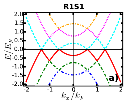
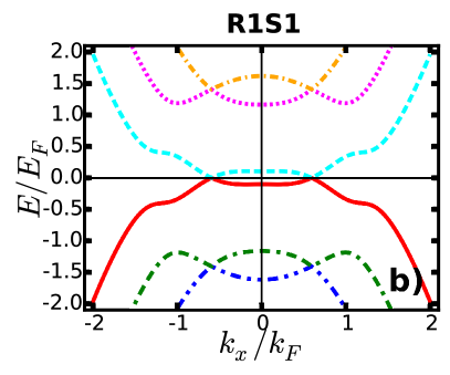
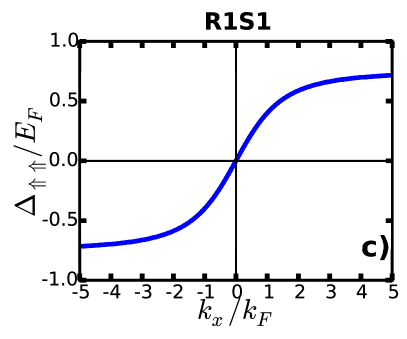
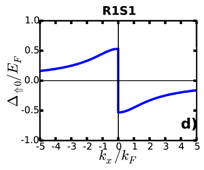
Figure 4: (Color online) The quasi-particle and quasi-hole energies versus momentum $k_{x}$ at $T=0.02E_{F}$ are shown in a) for $\Delta=0$ and in b) for $\Delta\neq 0$, corresponding to the phase $R1S1$ with $\Omega/E_{F}=0.79$ and $1/(k_{F}a_{s})=0.23$. The quasi-particle energies are shown as dot-dashed gold, dotted purple, and dashed cyan lines. The quasi-hole energies are shown as double-dot-dashed blue, double-dash-dotted green, and solid red. The corresponding order parameter tensor components $\Delta_{\Uparrow\Uparrow}({\bf k})$ and $\Delta_{\Uparrow 0}({\bf k})$ versus $k_{x}$ are shown in c) and d).

We have studied the quantum phases of interacting three component fermions in the presence of spin-orbit coupling and Zeeman fields. We classified the emerging superfluid phases in terms of the the loci of zeros of their quasi-particle excitation spectrum in momentum space, and identified several Lifshitz-type topological transitions. In the particular case that the quadratic Zeeman field is zero, a quintuple point exists where five gapless superfluid phases with surface and line nodes converge into a fully gapped superfluid phase. Lastly, we also showed that the simultaneous presence of spin-orbit and Zeeman fields transforms a momentum-independent scalar order parameter into an explicitly momentum-dependent tensor in the generalized helicity basis.

References

• (1) L. Landau and E. M. Lifshitz, Quantum Mechanics: Non-Relativistic Theory, Pergamon Press, London (1980).
• (2) M. Z. Hasan and C. L. Kane, Rev. Mod. Phys. 82, 3045 (2010).
• (3) X. L. Qi and S. C. Zhang, Rev. Mod. Phys. 83, 1057 (2011).
• (4) E. Bauer, and M. Sigrist, Non-centrosymmetric superconductors: Introduction and Overview, Springer-Verlag, Berlin (2012).
• (5) Y. J. Lin, K. Jimenez-Garcia, and I. B. Spielman, Nature (London) 471, 83 (2011).
• (6) R. A. Williams, M. C. Beeler, L. J. LeBlanc, K. Jimenez-Garcia, and I. B. Spielman, Phys. Rev. Lett. 111, 095301 (2013).
• (7) Z. Fu, L. Huang, Z. Meng, P. Wang, L. Zhang, S. Zhang, H. Zhai, P. Zhang, and J. Zhang, Nat. Phys. 10, 110 (2014).
• (8) M. Chapman and C. Sá de Melo, Nature (London) 471, 41 (2011).
• (9) C. J. Wu, I. M. Shem, X. F. Zhou Chin. Phys. Lett 28, 097102 (2011).
• (10) T. L. Ho and S. Zhang, Phys. Rev. Lett. 107, 150403 (2011).
• (11) Y. Li, L. P. Pitaevskii, and S. Stringari, Phys. Rev. Lett. 108, 225301 (2012).
• (12) J. P. Vyasanakere, S. Zhang, and V. B. Shenoy, Phys. Rev. B 84, 014512 (2011).
• (13) M. Gong, S. Tewari, and C. Zhang, Phys. Rev. Lett. 107, 195303 (2011).
• (14) Z.-Q. Yu and H. Zhai, Phys. Rev. Lett. 107, 195305 (2011).
• (15) H. Hu, L. Jiang, X.-J. Liu, and H. Pu, Phys. Rev. Lett. 107, 195304 (2011).
• (16) L. Han and C. A. R. Sá de Melo, Phys. Rev. A 85, 011606(R) (2012).
• (17) K. Seo, L. Han, and C. A. R. Sá de Melo, Phys. Rev. Lett. 109, 105303 (2012).
• (18) J. P. A. Devreese, J. Tempere, and C. A. R. Sá de Melo, Phys. Rev. Lett. 113, 165304 (2014).
• (19) N. Goldman, I. Satija, P. Nikolic, A. Bermudez, M. Martin-Delgado, M. Lewenstein, and I. B. Spielman, Phys. Rev. Lett. 105, 255302 (2010).
• (20) D. M. Kurkcuoglu, Ph. D. Thesis, Georgia Institute of Technology, (2015).
• (21) D. L. Campbell, R.M. Price, A. Putra, A. Valdés-Curiel, D. Trypogeorgos, and I.B. Spielman, Nat. Commun. 7, 10897 (2016).
• (22) I.M. Lifshitz, Zh. Eksp. Teor. Fiz. 38, 1569 (1960) [Sov. Phys. JETP 11, 1130 (1960)].