Evolving Powergrids in Self-Organized Criticality: An analogy with Sandpile and Earthquakes

Abstract

The stability of powergrid is crucial since its disruption affects systems ranging from street lightings to hospital life-support systems. Nevertheless, large blackouts are inevitable if powergrids are in the state of self-organized criticality (SOC). In this paper, we introduce a simple model of evolving powergrid and establish its connection with the sandpile model, i.e. a prototype of SOC, and earthquakes, i.e. a system considered to be in SOC. Various aspects are examined, including the power-law distribution of blackout magnitudes, their inter-event waiting time, the predictability of large blackouts, as well as the spatial-temporal rescaling of blackout data. We verified our observations on simulated networks as well as the IEEE 118-bus system, and show that both simulated and empirical blackout waiting times can be rescaled in space and time similarly to those observed between earthquakes. Finally, we suggested proactive maintenance strategies to drive the powergrids away from SOC to suppress large blackouts.

I Introduction

Self-organized criticality (SOC) corresponds to the mechanism a system self-organizes itself to achieve a critical state between different phases in the long run. It was first proposed by Bak et al in their seminal papers bak87 ; bak88 as the mechanism underlying the characteristic $1/f$ power-spectrum press87 , self-similar fractal structures mandelbrot82 as well as power-laws markovic14 , commonly observed in many different natural and artificial systems, across an extensive temporal and spatial scale bak89 . Although alternative approaches have been suggested to produce similar phenomena falconer04 ; sornette06 ; markovic14 , SOC was considered by some researchers to be the explanation for universal complexity in nature bak96 , although this view is under strong debate watkins16 .

Despite the strong debate, SOC has triggered tremendous interest in various areas including physics, biology, astronomy, geology and economics. Especially, many systems in these areas exhibit a power-law distribution of fluctuations, spanning from minimal disturbances to system-wide extreme events bak91 . These observations are consistent with those observed in the sandpile model bak87 ; bak88 , a prototype of SOC, in which the addition of a single sand grain may lead to avalanches of any magnitude following a power-law distribution. These similarities have made sandpile model (as well as SOC) a good analogy for explaining extreme events in the other systems, ranging from earthquakes bak02 and forest fires drossel92 on the earth to solar flares on the sun lu91 ; from mass extinction events in ancient nature bak93 to stock market crashes in modern society stauffer99 .

In this paper, we will examine another type of extreme event which significantly impacts our daily life – large blackouts caused by cascading failures in powergrids buldyrev10 . As an example of their negative impact, the large blackout in August, 2003 in USA contributed to 90 deaths anderson12 and was estimated to cost $\$$6.4 billion anderson03 . Similar to other extreme events, blackouts were shown to follow power-law size distributions carreras04 and SOC has been suggested to be the underlying mechanism dobson07 . In particular, the continual effort to satisfy the increasing consumption by upgrading the powergrids incrementally may have put it at a critical loading marginally before the emergence of the phase with frequent blackouts, i.e. the system is in SOC dobson07 . A model to demonstrate this idea was recently introduced in hoffmann14 . Nevertheless, most of these studies only focus on the power-law cascade size distributions, while other phenomena and consequences of powergrids as SOC systems are not examined.

The goal of this paper is to introduce a simple model of an evolving powergrid, i.e. a powergrid which serves a group of nodes with increasing energy demand, and upgrades its capacity everytime after an overloading failure. We will focus on the evolution of the powergrids beyond the extensively studied individual cascading failures motter02 . In addition to the cascade size distribution, we will examine the distribution of waiting time between blackouts, the predictability of large blackouts as well as the spatial-temporal rescaling of blackout data bak02 ; corral04 . We aim to show the connection between our model and (i) real powergrids, (ii) the sandpile model and hence SOC, and (iii) earthquakes (a potential candidate of SOC bak02 ); indirect connections between these three systems are then established. We tested our model on a real powergrid topology of the IEEE 118-bus system and obtained similar results. We also showed that real blackout data can be rescaled in space and time as we observed for earthquakes corral04 . Finally, we examined various maintenance strategies and their ability to suppress large blackouts by driving the system away from SOC.

II Model

We will introduce a model of evolving powergrid and shows its connection with the sandpile model bak87 ; bak88 . Specifically, we consider a network with $N$ nodes, labeled by $i=1,\dots,N$, where each node $i$ is connected with $k_{i}$ neighbors. Initially, a load $L_{i}$ is allocated to node $i$. A fraction $r$ of the nodes are considered as power stations and are assigned with a negative infinite load. The rest of the nodes are considered as energy consumers and are assigned a random positive load, which follows a normal distribution with a positive mean, truncated by discarding the negative side. Each node $i$ with a positive $L_{i}$ is required to acquire a sufficient amount of power from the power stations to satisfy its demand, i.e.

$$\sum_{j}A_{ji}I_{ji}=L_{i},$$ (1)

where $A_{ji}$ is the matrix element of the $N\times N$ adjacency matrix ${\cal A}$, such that $A_{ij}=1$ if nodes $i$ and $j$ are connected and otherwise, $A_{ij}=0$; the current $I_{ji}$ is the power flow from node $j$ to node $i$. We will implement the model on square lattices and a real powergrid topology.

To satisfy the demand of the consumer nodes, power is transferred to them from the power plants via the powergrid, composed of $M$ transmission lines called links. We adopt the direct current (DC) approximation and assume that currents on the links minimize the resistive power $\sum_{ij}A_{ij}I_{ij}^{2}R_{ij}$ in transportation, where $R_{ij}$ is the resistance on link $(ij)$. To simplify the model, we assume that $R_{ij}=1$ for all links, but the results can be easily generalized to the case with $R_{ij}\neq 1$. As shown in wong06 , the optimal current can be computed by solving the potential of each nodes, denoted as $v_{i}(t)$ for node $i$, given by wong06

$$v_{i}(t)=\max\left[\frac{1}{k_{i}}\left(\sum_{j}A_{ij}v_{j}(t)+L_{i}(t)\right),0\right].$$ (2)

Since Eq. (2) is a set of coupled equations involving a node and its neighbors, one can solve for $v$’s for all nodes by iterating the equations on the network until convergence wong06 . The optimal current $I_{ij}(t)$ from node $j$ to node $i$ on a link $(ij)$ is then given by $I_{ij}(t)=v_{i}(t)-v_{j}(t)$, and $I_{ij}(t)=-I_{ji}(t)$.

Since links are transmission lines which may break when overloaded, we define the capacity of link $(ij)$ to be $C_{ij}(t)$ and consider that the link fails and no longer transfers electricity if the current $|I_{ij}|>|C_{ij}|$. Initially at time $t=0$, the capacity $C_{ij}(0)$ of a link $(ij)$ is defined as

$$C_{ij}(0)=(1+\alpha)I_{ij}(0),$$ (3)

where $I_{ij}(0)$ is the optimal current of the link at time $t=0$, while $\alpha$ is the ratio of excess capacity installed in the network, which we call the redundancy ratio. The capacity plays a role similar to the threshold in the sandpile model beyond which sands topple to the neighboring sites. Unlike the sandpile model, the capacity in the powergrid evolves with time due to repairs after a failure, given by

$$C_{ij}(t+1)=(1+\alpha){\tilde{I}}_{ij}(t),$$ (4)

where ${\tilde{I}}_{ij}(t)$ is the current which breaks the link. Capacities are heterogeneous across the network, which are different from the homogeneous thresholds in other SOC models such as the sandpile model, the OFC earthquake model olami92 and the powergrid model in hoffmann14 . Yet, as we will see, this heterogeneity does not destroy criticality in our model, unlike that observed in the OFC model janosi93 .

To model the increase in the demand for electricity, we randomly pick a consumer node at time $t$ and increase its demand by

$$L_{i}(t)=L_{i}(t-1)+\beta\langle L_{i}(t-1)\rangle,$$ (5)

where $\langle L_{i}(t)\rangle=\sum_{j=1}^{N}L_{j}(t)/N$ and $\beta$ is the demand increment ratio. This is analogous to the addition of sands to the sandpile model. After each demand increment, the new optimal currents are computed by iterating Eq. (2), and links with currents exceeding the capacity are considered broken and removed from the powergrid. Currents are then re-computed and new broken links are identified, leading to a cascading failure as shown in Fig. 1(a) and (b); some nodes may become disconnected from the powergrid as shown in Fig. 1(c). But unlike the sandpile model, a failed link may affect links other than the nearest ones, as shown in the transition from Fig. 1(a) through (c). The process repeats until no extra link breaks, and all failed links are then repaired according to Eq. (4). The whole cascading failure and repairs are finished within one time step before the next demand increment, which corresponds to a fast relaxation dynamics intercepting a slow driving dynamics, an essential mechanism in many SOC systems bak96 . As the procedures repeat, a series of cascading failures is observed. In this paper, we call a failure a blackout regardless of its size.

(a)		(b)		(c)		(d)
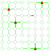
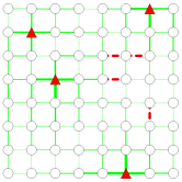
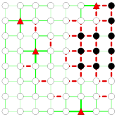
			$\cdots$		$\cdots$
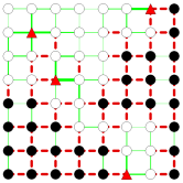
Cascade Step=1		Cascade Step=2		Cascade Step=4		Cascade Step=6

Figure 1: The dynamics of a cascading failure, or a blackout, in our model. Power stations and consumer nodes are denoted as triangles and circles, respectively. Shaded circles correspond to consumer nodes which are disconnected from the power stations due to the failed links. (a) A link in the network is broken after a demand increment. (b) and (c) Power transmitted by the broken link is shared by the other links, which overload the other links to the same power station and render it isolated; the load in the network are now shared by the remaining power stations, leading to failures in areas away from the initially failed link. (d) The end of the cascade and all the failed links in this single blackout.

To keep the model simple, we set $\alpha=\beta$ such that the rates of load and capacity increment are equal. In this case, the model only captures the most essential components of the system to illustrate its relevance with SOC. While capacities and loads monotonically increase, we rescale all loads and capacities by the same factor after a number of simulation time steps to keep all the variables finite; the dynamics between the variables does not change since all equations involving loads and capacities are linear. Since we will focus on the SOC phenomenon in this paper, the analyses of the system behaviors with different $\alpha$ are given in the Appendix C.

III Results

III.1 Self-organized criticality in the model powergrid

To show that our powergrid model exhibits the characteristics of a critical state, we first examine the distribution of cascade size, measured as the total number of broken links in a failure. As shown in Fig. 2, the cascade size follows a power-law distribution similar to the empirical results dobson07 . Although different tails are observed for cases with different model parameter $\alpha$, we remark that a universal power-law exponent is observed with $\alpha$ spanning two order of magnitudes from $0.01$ to $3.2$, which emerges from self-organization without fine-tuning, suggesting universality independent of model parameters. On the other hand, as shown in the inset of Fig. 2, the cascade size distributions for different system sizes also follow power-laws with the same exponent where the cutoff increases with system size, suggesting scale invariance typical of critical systems.

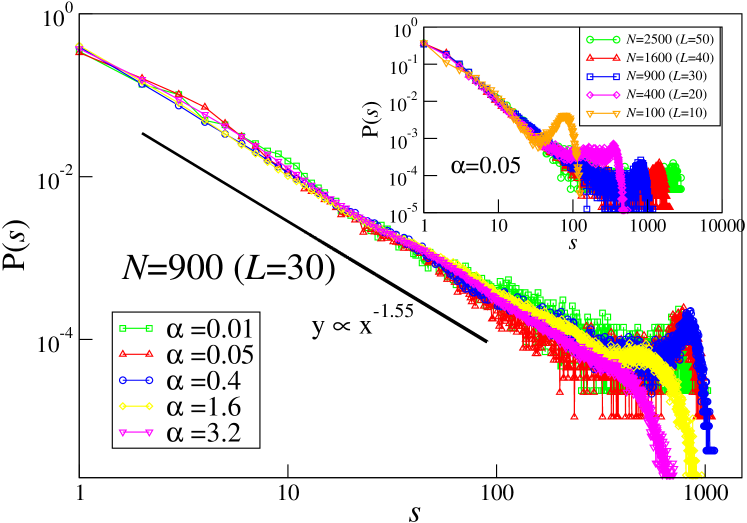
Figure 2: The distribution of cascade size, i.e. the total number of broken links in each failure, obtained on $L\times L$ square lattices with $L=30$ and $N=L^{2}=900$ nodes, with $5\%$ of the nodes to be power station. The statistics is obtained for at least $N\times 2\times 10^{3}$ updates after an equilibration of $N\times 10^{2}$ updates. Inset: The distributions of cascade size with different system size $N$ with $\alpha=0.05$.

To further examine the criticality of our powergrid model, we compute the distribution of waiting time $T$ between consecutive failures. Since avalanches in SOC systems are unpredictable, their waiting time distributions should follow an exponential decay, though it is not common to use merely the exponential waiting time distribution to justify SOC sanchez02 ; boffetta99 ; aschwanden11 . As shown in the semi-log plot in Fig. 3(a), the waiting time distributions for the cases with different $\alpha$ follow an exponential decay. The distributions in log-log plot in Fig. 3(b) show that they resemble the empirical results observed in real powergrids dobson07 , and earthquakes corral04 except a more prominent power-law at the small time scale contributed by the correlated aftershocks after a main shock described by the Omori’s Law omori1894 . After-blackouts do not occur in our model and instead, failures occur less frequently after a large blackout since a large number of links were repaired simultaneously.

To examine the predictability of the occurrence and the size of blackouts, we analyze the sequence of waiting times and cascade sizes by detrended fluctuation analysis (DFA); detailed description of DFA is found in the Appendix A. As shown in Fig. 9 and Fig. 10, the behavior of the sequence of waiting times and cascade sizes is analogous to that of the corresponding reshuffled sequence when a small number of consecutive blackouts are considered. This implies that the exact behavior of blackout occurrence is unpredictable in the short time scale. On the other hand, the behavior of the sequences deviates from that of the reshuffled one when a large number of consecutive blackouts are considered; it implies that the emergence of blackouts become more predictable in the long run, e.g. a large blackout or a long waiting time emerges when a sufficiently long sequence of blackouts is considered. Nevertheless, the larger the system size, the longer the time scale which is consistent with the reshuffled results, implying a lower predictability in larger systems.

Stimulated by the DFA results, we examine the presence of blackout precursors. We first divide the time between consecutive pairs of large blackouts into a fixed number of divisions, and compute statistics within each division to identify potential trends. As shown in Fig. 4(a), the failure rate increases and drops before the emergence of medium blackouts with size $s\geq 0.1M$ and $s\geq 0.3M$, where $M$ is the total number of links, which may signal an insufficient relaxation of energy before the blackouts. On the other hand, the failure rate increases continuously before blackouts of size $s\geq 0.5M$, which may be caused by a sequence of medium-sized blackouts (suggested by the large average blackout size) relaxing energy incompletely, and finally triggered by a sequence of small but more frequent blackouts, indicating a close-to-critical state of the system.

Nevertheless, Fig. 4(a) shows the average failure rate while individual events may be unpredictable by just examining the preceding sequence of blackouts. Prediction may instead be possible if the microscopic information of the system is available. To examine this predictability, we define the load factor of link $(ij)$ to be $F_{(ij)}=|I_{ij}|/C_{ij}$, and compute the average network load factor $F$ given by

$$F=\frac{1}{M}\sum_{(ij)}F_{ij}=\frac{1}{M}\sum_{(ij)}\frac{|I_{ij}|}{C_{ij}}.$$ (6)

A small value of $F$ implies a large amount of redundant capacity and failures are less likely. As shown in Fig. 4(b), $F$ increases between two large blackouts, and a high $F$ may be a signal for coming large failures. These results suggest that prediction is difficult given only macroscopic information, e.g. the sequence of failures, but may be possible if microscopic information in the system is available. This is analogous to the predictability of earthquakes suggested in bernard01 .

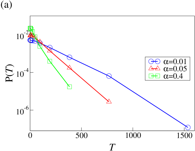
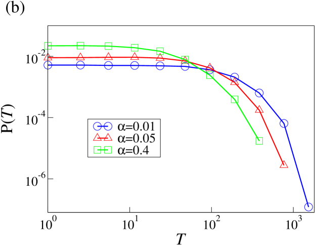
Figure 3: The distributions of waiting time between consecutive blackouts of size $s\geq 1$, obtained on an instance of $L\times L$ square lattice with $L=30$ and $N=L^{2}=900$ nodes, with $5\%$ of the nodes to be power stations, in (a) semi-log plot and (b) log-log plot. The statistics is obtained for $N\times 10^{4}$ updates after an equilibration of $N\times 10^{2}$ updates. To better show the form of the distributions, log-bins are used to obtain the distributions.

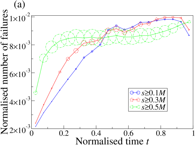
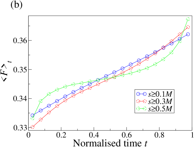
Figure 4: (a) We divide the duration between consecutive pairs of large blackouts into 20 divisions and compute the failure rate within each division averaged over different pairs of large blackouts with size $s\geq 0.1M$, $0.3M$ and $0.5M$. The size of the nodes corresponds to the average blackout size in that particular division. The results are averaged over 27 realizations of $L\times L$ square lattice with $L=30$ and $N=L^{2}=900$ nodes, with $5\%$ of the nodes being power stations. The statistics is obtained for $N\times 10^{4}$ updates after an equilibration of $N\times 10^{2}$ updates. (b) The corresponding average network load factor $F$ given by Eq. (6).

As suggested by bak87 ; bak88 ; watkins16 , spatio-temporal correlation is an important feature of SOC systems since it connects the dynamical self-organization with spatial criticality. To examine this correlation, we consider a $l\times l$ partition (details are shown in Appendix B), and define $P_{S,l}(T)$ to be the waiting time distribution within the partition between blackouts with size $s>S$. As shown in Fig. 5(a), an increase in the cutoff size $S$ (or a decrease in partition size $l$) makes the distributions wider, compared to the original $P_{S=1,l=20}(T)$. Hence, it is interesting to examine if the statistics of large failures in large partitions are equivalent to those of small failures in small partitions. We follow the analyses of earthquakes in bak02 , and plot the rescaled distributions $T^{\gamma}P_{S,l}(T)$ as a function of the rescaled waiting time $x=TS^{-b}l^{d_{f}}$ in Fig. 5(b), such that $P_{S,l}(T)$ with various $S$ and $l$ collapse onto the same function $f(x)$, i.e.

$$T^{\gamma}P_{S,l}(T)=f(TS^{-b}l^{d_{f}}).$$ (7)

As suggested in bak02 , $\gamma$, $b$ and $d_{f}$ corresponds to the exponents of the Omori’s Law, the exponent of the cumulative distribution of shock magnitude (i.e. the exponent of Gutenberg-Richter Law gutenberg54 ), and the fractal dimension of earthquakes, respectively. In our case, $\gamma=1.07$, $b=0.54$ and $d_{f}=1.5$, and the value $-b-1$ is consistent with the exponent $\approx-1.54$ in the blackout size distribution in Fig. 2, consistent with relation suggested by Bak et al for empirical earthquake data bak02 . This data collapse in Fig. 5(b) suggests that waiting times between blackouts in our model can be rescaled in spatial and temporal dimension, again suggesting universality, and is similar to that observed for earthquakes.

   

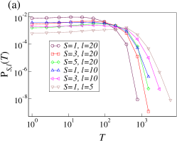
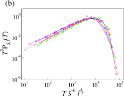
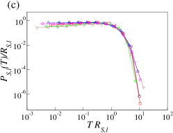
Figure 5: (a) The distribution $P_{S,l}(T)$ of waiting time $T$ between consecutive failures with size $s\geq S$ in a $l\times l$ partition of the network, for different values of $S$ and $l$. (b) The data collapse of all the distributions in (a) by plotting $T^{\gamma}P_{S,l}(T)$ as a function of $x=TS^{-b}l^{d_{f}}$, suggested in bak02 for earthquakes, with $\gamma=1.07$, $b=0.54$ and $d_{f}=1.5$. (c) The data collapse of all the distributions in (a) by plotting $R_{S,l}^{-1}P_{S,l}(T)$ as a function of the rescaled waiting time $x=R_{S,l}T$, suggested in corral04 for earthquakes, where $R_{S,l}$ is the average event rate with size $s\geq S$ in the partition of size $l$. The results are obtained on $L\times L$ square lattices with $L=20$ and $N=L^{2}=400$ nodes, with $5\%$ of the nodes to be power stations. The statistics is obtained for $N\times 3\times 10^{5}$ updates after an equilibration of $N\times 10^{2}$ updates.

To further examine the universality of blackout waiting time in our model, we follow an alternative form of rescaling proposed by corral04 . By drawing again an analogy with earthquakes, the distributions $P_{S,l}(T)$ with various $S$ and $l$ for blackouts collapse onto the function $g(x)$ as shown in Fig. 5(c), i.e.

$$R_{S,l}^{-1}P_{S,l}(T)=g(R_{S,l}T),$$ (8)

where $R_{S,l}$ is the average blackout frequency in the partition. The two data collapses in Fig. 5(b) and (c) may suggest that scale invariance and universality emerge in our model of powergrid, resembling those observed for earthquakes bak02 ; corral04 . All the above results suggest that our powergrid model results in a realistic blackout statistics as well as the characteristics of self-organized criticality.

IV SOC on real powergrids

To examine the robustness of the SOC phenomenon against network topology, we implement our model on the IEEE 118-bus system, which represents a portion of the American Electric Power System in the Midwestern US as of December, 1962 118system . Before the simulation starts, we assign a load $L_{i}$ to each consumer node $i$ according to its load given in 118system ; power stations are assigned with an infinite amount of resources. The system then follows the same dynamics described in our model. As shown in Fig. 6(a), the cascade size distribution roughly follows a power-law with the same exponent observed on square lattices. The waiting time distribution is also similar to those observed on square lattices and empirical results dobson07 . These suggest that SOC behaviors may also emerge on real powergrid topologies following our model dynamics.

To further examine the robustness of the SOC behaviors in the IEEE 118-bus system, we re-allocate the power stations randomly and examine the system behaviors. As shown in Fig. 6(a), the distribution of failures still roughly follows a power-law but large failures are more likely. These results show that powergrid failures are more strongly dependent on the location of power stations than the topology of the system. With an appropriate allocation of power stations, large failures are more suppressed since the original load from a broken link can be shared evenly to the other links. Unlike the sandpile model composed of all identical nodes, power stations in powergrids play a crucial role and their locations impact the system behaviors. Nevertheless, regardless of the location of the power stations, the system still shows a general picture consistent with SOC.

In addition to the simulations on a real powergrid topology, we also examine the spatial-temporal rescaling using the empirical data of waiting times, obtained from the data spanning 15 years of power outages across the United State  realdata . Since the data do not show the failure of individual links in a blackout, we cannot identify blackouts according to partitions as in bak02 (see Appendix B), but the rescaling according to Eq. (8) by the average failure rate is feasible corral04 . As shown in Fig. 6(b), the rescaled waiting time distributions with different cutoff size $S$ overlap on a common function, similar to those observed in simulations in Fig. 5(c). This again suggests that the empirical results are consistent with the simulated results, and SOC is a potential mechanism underlying real powergrids.

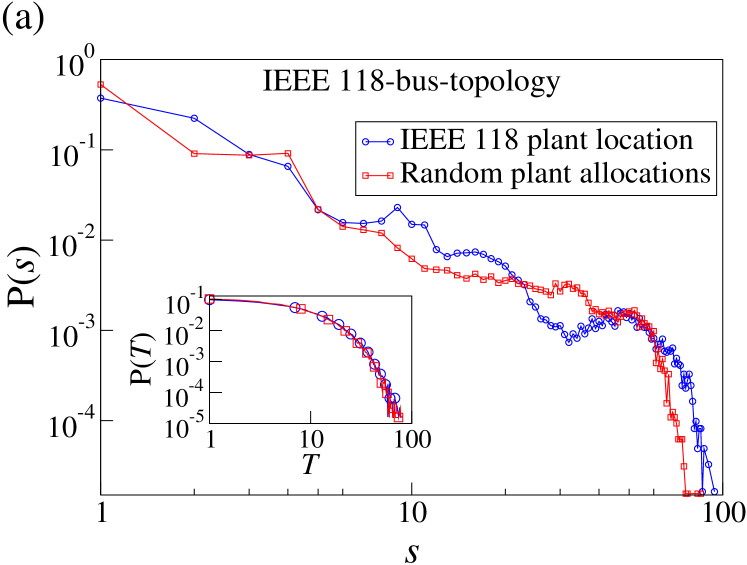
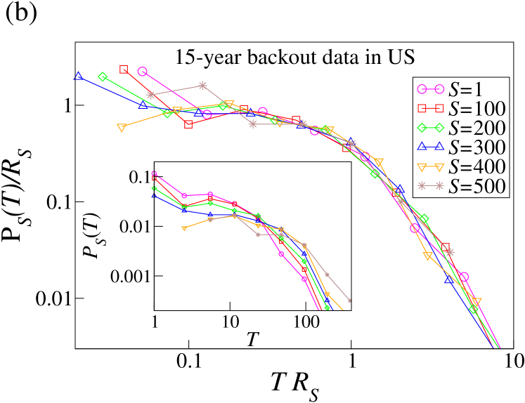
Figure 6: (a) The distributions of blackout size, obtained on the IEEE 118-bus system with $N=118$, 105 consumer nodes, $15$ power stations and 186 links. Blue circles and red squares correspond to the cases where power stations are located at the original location and random location, respectively. The statistics is obtained for $N\times 10^{4}$ updates after an equilibrium of $N\times 10^{2}$ updates. Inset: The waiting time distributions of the two cases. (b) The rescaled waiting time distributions of the 15-year data of power outages across the United State realdata , $R_{S}^{-1}P_{S}(T)$ as a function of the rescaled waiting times $x=R_{S}T$, where $R_{S}$ is the average occurrence rate of failure of size greater than $S$. Inset: The waiting time distributions of the 15-years data of power outages across the United State with failure of size $s>S$.

V Escaping SOC by proactive maintenance

If a powergrid is in SOC, large blackouts and their negative impacts anderson12 ; anderson03 are inevitable. As we have seen, the system does not escape form SOC by repairing the broken links after failures, instead this mechanism leads to criticality. Compared with the non-controllable earth crust movement underlying earthquakes, powergrids are composed of controllable components, and therefore, to avoid large blackouts, one can implement microscopic interventions to drive the system away from SOC. In addition to the remedial repairs, we will explore three proactive maintenance approaches to increase link capacity in advance of large failures:

1. Maintenance based on the global load factor - at each step without failure, given the average network load factor $F$ is larger than a threshold $\psi$, i.e. $F>\psi$ (see Eq. (6)), the capacity of the link with the highest individual load factor, i.e. the link $(ij)=\operatorname*{{\rm{argmax}}}_{(ij)}[F_{(ij)}]$, is upgraded by $C_{ij}^{\prime}(t)=C_{ij}(t)(1+\alpha)$; the above procedure is repeated within a time step until $F<\psi$;

2. Maintenance based on local load factors - at each step without failure, we increase the capacity of all links $(ij)$ if their load factor exceeds the threshold $\psi$, i.e. to upgrade $C_{ij}^{\prime}(t)=\frac{I_{ij}(t)}{\psi}$ when $F_{(ij)}>\psi$, so that $F_{(ij)}$ falls to $\psi$;

3. Routine maintenance - the capacities of the $n$ links with the highest load factor are upgraded by $C_{ij}(t+1)=C_{ij}(t)(1+\alpha)$.

We first discuss the results of the first approach. As shown by the blue ($\Box$) and green ($\bigcirc$) curves respectively in Fig. 7(a), for $\psi<0.2$, a large amount of extra capacity is required in proactive maintenance, but only a small amount of extra capacity is required to repair the broken links since blackouts are rare as shown in Fig. 7(c); the system escapes from SOC. When $\psi$ increases from $\psi=0.2$ to $\psi=0.25$, less extra capacity is required for maintenance but more capacity is used for repairing the failed links. Beyond $\psi\approx 0.25$, the amount of extra capacity required for proactive maintenance almost vanishes, which indicates that the global load factor $F$ seldom reaches $\psi$ to activate the proactive procedures; this may also mark the typical load factor which triggers the failures. The system returns to SOC and further reduces to the original no-maintenance case when $\psi\rightarrow 1$.

Interestingly, compared with the original case without maintenance (i.e. $\psi\rightarrow 1$), (i) the total amount of extra capacity required for all interventions (i.e. proactive maintenance or remedial repairs) is less and attains a minimum at $\psi\approx 0.2$, and (ii) at the same time failures are less frequent, as shown in Fig. 7(a) and (c) respectively. It is because maintenance leads to an even distribution of redundant capacity, compared with the biased distribution of excessive capacity on individual heavily loaded links after failures. However, a large number of maintenance is required in this approach as shown in Fig. 7(b), resulting in a trade-off between the required amount of extra capacity and the required number of interventions (i.e. the total number of maintenance and repairs) to sustain the system as shown in Fig. 8.

We then discuss the second and the third maintenance approach. As shown in Fig. 7(d) - (f), the second approach behaves similarly as the first approach, except that a much larger number of interventions (mainly maintenance) are required in exchange for a smaller amount of extra required capacity (see also Fig. 8). On the other hand, as shown in Fig. 7(g) and (h), the third approach requires only a small amount of extra capacity achieved by a small number of interventions, outperforming both the first and the second approach. Nevertheless, it is less effective in eliminating failures as shown Fig. 7(i) unless $n\gtrsim 3$ at which much more extra capacity are required. A better comparison is shown in Fig. 8, where the third approach - a simple routine maintenance - is the most cost-effective approach to drive the system away from SOC. In summary, all three approaches suppress blackouts and at the same time use less extra capacity compared with the original case without proactive maintenance.

We remark that powergrids with proactive maintenance may share similarities with the non-conserving variants of SOC models olami92 ; drossel92 , in which the SOC characteristics are lost. While the former extends capacity in advance to suppress blackouts, the latter dismisses a fraction of energy during toppling to suppress avalanches, leading to subcritical behaviors in both kinds of systems broker97 ; pruessner02 . As a result, proactive maintenance are effective to suppress large failures since they drive the system away from SOC.

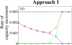
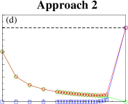
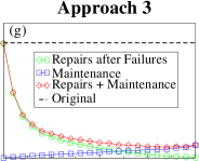
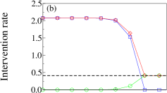
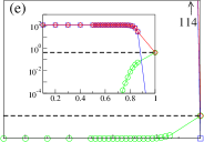
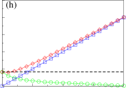
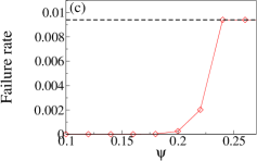
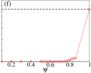
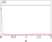
Figure 7: (a, d, g) The rate of capacity increment, (b, e, h) the intervention rate (i.e. the average number of maintenance and repairs per step), and (c, f, i) the failure rate of the system, by applying the three maintenance approaches. The results are obtained by averaging 5 realizations of $L\times L$ square lattice with $L=30$ and $N=L^{2}=900$ nodes, with $5\%$ of the nodes to be power stations. The statistics is obtained for $N\times 10^{2}$ updates after an equilibration of $N\times 10^{4}$ updates.

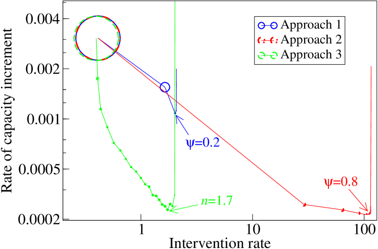
Figure 8: The trade-off between the rate of capacity increment and the intervention rate of the three proactive maintenance approaches. The size of the nodes corresponds to the rate of blackouts.

VI Discussion

Powergrids were suggested to be in self-organized criticality (SOC). To verify the conjecture, we introduced a model of powergrids which constantly evolves and upgrades to satisfy the increasing energy demand, resulting in a dynamics of intermitten failures and recovery. The model demonstrates various SOC characteristics and an analogy to earthquakes. Some of these findings are verified by implementation on real powergrid topology and empirical data. The model behaviors and the data analyses provide further evidences to suggest that an evolving powergrid is in SOC.

If powergrids are in SOC, what are the consequences? Large blackouts are inevitable and unpredictable. Since they have a great negative impact, it is essential to suppress them, and the way to achieve the goal is to drive the system away from SOC, or otherwise it self-organizes to criticality again. Unlike earthquakes which involve the non-controllable earth crust, powergrids are composed of controllable components; intervention may greatly increase the predictability and controllability of blackouts. Several proactive maintenance approaches are suggested in additional to the ordinary remedial repairs, and are shown to be effective in suppressing SOC and large blackouts. While the present study focuses on powergrids, its strong connection with SOC would make the results relevant to other SOC systems, especially in terms of controllability.

VII Acknowledgement

CHY acknowledges the Dean’s Research Fund 04115 ECR-5 2015 of the Hong Kong Institute of Education and the Research Grants Council of Hong Kong (ECS Grants No. 28300215). AZ is supported by the National Natural Science Foundation of China (Grant No. 11547188) and the Young Scholar Program of Beijing Normal University(Grant No. 2014NT38). KYMW is supported by a grant from the Research Grants Council of Hong Kong (grant number 605813).

The author declares no competing financial interests.

APPENDIX A: Detrended fluctuation analysis

We employ the detrended fluctuation analysis (DFA) hu01 ; lennartz08 to examine the long term memory, i.e. persistence or anti-persistence, of the sequence of waiting time between blackouts, and the size of the blackouts. Given a time series $x(i)$, with $i=1,2,\cdots,N$, we first define the cumulative sequence $y_{i}$ to be

$$y(i)=\sum_{j=1}^{i}(x(j)-\left<x\right>),$$ (9)

where $i=1,2,\cdots,n$, and $\left<x\right>$ is the expected value for the whole sequence $x(i)$, given by

$$\left<x\right>=\frac{1}{N}\sum_{i=1}^{N}x(i).$$ (10)

We then divide the whole sequence into $\lfloor\frac{N}{n}\rfloor$ time window of equal size $n$. In each time window, we best-fit the cumulative sequence in the window with a $l$-th order polynomial function $y_{fit}(i)$ given by

$$y_{fit}(i)=\sum_{k=0}^{l}\beta_{k}i^{k}$$ (11)

where $\beta_{k}$’s are the coefficient of the polynomial, and $y_{fit}(i)$ is thus the local trend in the window. We call the analyses $l$-DFA given an $l$-th order polynomial is used as the fit.

We then compute the detrended fluctuation function ${\cal F}(n)$ for time window length $n$, by detrending the cumulative sequence, i.e. subtracting $y(t)$ in each window by the corresponding local trend $y_{fit}(i)$, i.e.

$$z(i)=y(i)-y_{fit}(i).$$ (12)

For each window length $n$ , we calculate the root-mean-square deviation from the trend as the detrended fluctuation function ${\cal F}(n)$, given by

$${\cal F}(n)=\sqrt{\frac{1}{n}\sum_{i=1}^{n}(z(i))^{2}}.$$ (13)

We denote the average of ${\cal F}(n)$ over the different time window to be $\langle{\cal F}(n)\rangle$. By repeating the above processes for different values of $n=2^{k}$, with $k=1,\dots$, we obtain a relation between $\langle{\cal F}(n)\rangle$ and $n$. For a power-law relation $\langle{\cal F}(n)\rangle\propto n^{D}$, the sequence is random if $D=0.5$, anti-persistent if $D<0.5$, and persistent if $D>0.5$.

To examine the predictability of blackouts, we performed 0-DFA on the sequences of waiting times and the size of blackouts, and compare these results to the corresponding sequences after random reshuffling, i.e. a random re-order of the individual entry of the sequences. If there are no pattern on the sequences, the exponent $D$ should be consistent with those of the reshuffled sequences, and the waiting times and the size of blackouts are unpredictable. On the other hand, if the the exponent $D$ differs from that of the reshuffled sequence, then there are predictability in the sequences, i.e. either the sequences are persistent or anti-persistence. We remark that 1-DFA and 2-DFA were also performed and the results obtained are similar to those of 0-DFA, and thus we only present the results from 0-DFA.

Figure S9 shows ${\cal F}_{waiting}(n)$ as a function of $n$ obtained by 0-DFA for the sequence of the waiting times. Interestingly, ${\cal F}_{waiting}(n)$ seems to be characterized by two different power-laws. When $n$ is small ($n=2^{2}$ to $2^{5}$ for $L=20$, $n=2^{2}$ to $2^{6}$ for $L=30$ and $n=2^{2}$ to $2^{7}$ for $L=40$), $D=0.48,0.49,0.52$ for $L=20,30,40$ respectively, consistent with the corresponding reshuffled sequences. This implies that for a short sequence of blackouts, the waiting times are random and unpredictable. However, for a longer sequence of waiting times ($n=2^{6}$ to $2^{16}$ for $L=20$, $n=2^{7}$ to $2^{16}$ for $L=30$ and $n=2^{8}$ to $2^{16}$ for $L=40$), $D$ deviates from those of the reshuffled sequences and become $0.88,0.86,0.85$ for $L=20,30,40$ respectively. This suggests that persistence exists if we consider a long sequence of blackouts, i.e. there is a long waiting time which may be a consequence of a large blackout given a sufficiently long time. Moreover, the exponent $D$ changes abruptly, separating an unpredictable range ($D\approx 0.5$) from a predictable range ($D>0.5$). As we can see from Fig. 9, the larger the system size, the larger the values of $n$ where the system remains unpredictable, implying a lower predictability in larger systems.

Similar to waiting times, we performed 0-DFA on the sequence of blackout sizes. As shown in Fig. 10, ${\cal F}_{cascade}(n)$ is consistent with the corresponding reshuffled sequences at small $n$ ($n=2^{2}$ to $2^{3}$ for $L=20$, $n=2^{2}$ to $2^{4}$ for $L=30$ and $L=40$), where $D=0.79,0.87,0.87$ for $L=20,30,40$ respectively. This implies a persistent behavior in the sequence of blackout size, which may be a consequence of the memory in the loading factor, i.e. the network loading increases gentlely which leads to consecutive blackouts of similar size. We remark that such persistence is also observed for the reshuffled sequence, since small blackouts are much more common (see Fig. 2). For the intermediate range of $n$ ($n=2^{4}$ to $2^{7}$ for $L=20$, $n=2^{5}$ to $2^{8}$ for $L=30$ and $L=40$), $D=0.30,0.26,0.25$ for $L=20,30,40$ respectively, suggesting a slight anti-persistence. This may come from the cycle of blackouts, where large blackouts are usually followed by a period of small blackouts, due to the extensive repairing after a large blackout. Finally, at large $n$ ($n=2^{8}$ to $2^{16}$ for $L=20$, $n=2^{9}$ to $2^{16}$ for $L=30$ and $L=40$), $D$ increases again and becomes $0.83,0.82,0.81$ respectively for $L=20,30,40$, suggesting the occurrence of a large blackout given a sufficiently long time. Finally, the larger the system size, the larger the values of $n$ where the system remains unpredictable, similar to that observed for waiting times.

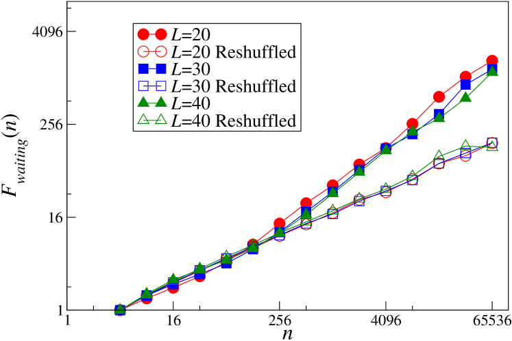
Figure 9: ${\cal F}_{\text{waiting}}(n)$ as a function of time window length $n$, for the original and the reshuffled sequence of waiting times for different system size $L$.

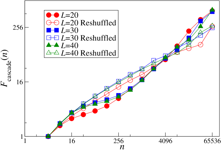
Figure 10: ${\cal F}_{\text{cascade}}(n)$ as a function of time window length $n$, for the original and the reshuffled sequence of blackout size for different system size $L$.

APPENDIX B: Partition for spatio-temporal rescaling of waiting time distribution

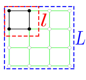
Figure 11: A partition of size $l\times l$ in a network with size $L\times L$.

To examine the spatio-temporal relation of the occurrence of blackouts in our model, we follow bak02 to rescale the waiting time distribution. We first group the nodes in the network into square partitions of size $l\times l$, as shown in Fig. 11. We then define the constituent links of a partition to be those with both terminal nodes located inside the partition. Since there is no epicentre in blackouts, we consider a failure has occurred in a partition when at least one of its constituent links breaks; the size of the failure is defined by the number of failed links within the partition. The waiting time in a partition is defined to be the time between consecutive failures in the partition. We further define a cutoff size $S$ such that only the waiting time between failures with size greater than or equal to $S$ is considered. Finally, we denote the waiting time distribution in a $l\times l$ partition with a cutoff size $S$ to be $P_{S,l}(T)$, such that $P_{S,l}(T)$ with various $S$ and $l$ collapse onto the same function given by Eq. (7). The original and the rescaled distributions are shown in Fig. 5 (a) and (b).

APPENDIX C: Waiting time as a function of Redundancy ratio

Figure 12: The average waiting time as a function of $\alpha$, obtained on $L\times L$ square lattices with $L=30$ and $N=L^{2}=900$ nodes, with $r=45$ of the nodes to be power station. The statistics is obtained for $1\times 10^{6}$ updates after an equilibration of $1\times 10^{5}$ updates.

Figure 13: The expected value of the average network load factor as a function of $\alpha$, obtained on $L\times L$ square lattices with $L=30$ and $N=L^{2}=900$ nodes, with $r=45$ of the nodes to be power station. The statistics is obtained for $N\times 10^{2}$ updates after an equilibration of $N\times 10^{4}$ updates.

We will discuss the waiting time between two failures as a function of the redundancy ratio $\alpha$. As shown in Fig. 12, the average waiting time starts at a high value at the smallest $\alpha$, decreases with $\alpha$, suggesting that the failure rate decreases with $\alpha$. As shown in Fig. 13, the average network load factor $\langle F\rangle$ (see Eq. (6)) increases as $\alpha$ increases, in a trend opposite to that of the average waiting time. These results imply that at the smallest $\alpha$ value, failures are less frequent since the demand increments are more gentle and the average network load factor $\langle F\rangle$ stays at a low value for a large amount of time. Increasing $\alpha$ in this regime would increase $\langle F\rangle$, which leads to an increase of failure rate, and hence a decrease in the average waiting time.

References

- (1) P. Bak, C. Tang, and K. Wiesenfeld, Physical review letters 59, 381 (1987).
- (2) P. Bak, C. Tang, and K. Wiesenfeld, Physical review A 38, 364 (1988).
- (3) W. H. Press, Comments on Astrophysics 7, 103 (1978).
- (4) B. B. Mandelbrot, The fractal geometry of nature (Macmillan, ADDRESS, 1983), Vol. 173.
- (5) D. Marković and C. Gros, Physics Reports 536, 41 (2014).
- (6) P. Bak and K. Chen, Physica D: Nonlinear Phenomena 38, 5 (1989).
- (7) K. Falconer, Fractal geometry: mathematical foundations and applications (John Wiley & Sons, ADDRESS, 2004).
- (8) D. Sornette, Critical phenomena in natural sciences: chaos, fractals, selforganization and disorder: concepts and tools (Springer Science & Business Media, ADDRESS, 2006).
- (9) P. Bak, How nature works (Springer, ADDRESS, 1996), pp. 1–32.
- (10) N. W. Watkins et al., Space Science Reviews 198, 3 (2016).
- (11) P. Bak and K. Chen, Scientific American (United States) 264, (1991).
- (12) P. Bak, K. Christensen, L. Danon, and T. Scanlon, Physical Review Letters 88, 178501 (2002).
- (13) B. Drossel and F. Schwabl, Physical Review Letters 69, 1629 (1992).
- (14) E. T. Lu and R. J. Hamilton, The Astrophysical Journal 380, L89 (1991).
- (15) P. Bak and K. Sneppen, Physical Review Letters 71, 4083 (1993).
- (16) D. Stauffer and D. Sornette, Physica A: Statistical Mechanics and its Applications 271, 496 (1999).
- (17) S. V. Buldyrev et al., Nature 464, 1025 (2010).
- (18) G. B. Anderson and M. L. Bell, Epidemiology (Cambridge, Mass.) 23, 189 (2012).
- (19) P. L. Anderson and I. K. Geckil, Anderson Economic Group (2003).
- (20) B. A. Carreras, D. E. Newman, I. Dobson, and A. B. Poole, Circuits and Systems I: Regular Papers, IEEE Transactions on 51, 1733 (2004).
- (21) I. Dobson, B. A. Carreras, V. E. Lynch, and D. E. Newman, Chaos: An Interdisciplinary Journal of Nonlinear Science 17, 026103 (2007).
- (22) H. Hoffmann and D. W. Payton, Chaos, Solitons & Fractals 67, 87 (2014).
- (23) A. E. Motter and Y.-C. Lai, Phys. Rev. E 66, 065102 (2002).
- (24) A. Corral, Physical Review Letters 92, 108501 (2004).
- (25) K. Y. M. Wong and D. Saad, Physical Review E 74, 010104 (2006).
- (26) Z. Olami, H. J. S. Feder, and K. Christensen, Physical Review Letters 68, 1244 (1992).
- (27) I. Janosi and J. Kertesz, Physica A: Statistical Mechanics and its Applications 200, 179 (1993).
- (28) R. Sánchez, D. E. Newman, and B. A. Carreras, Physical review letters 88, 068302 (2002).
- (29) G. Boffetta, V. Carbone, P. Giuliani, P. Veltri and A. Vulpiani, Physical review letters 83, 4662 (1999).
- (30) M. Aschwanden, Self-organized criticality in astrophysics: The statistics of nonlinear processes in the universe (Springer Science & Business Media, ADDRESS, 2011).
- (31) F. Omori, Journal of the College of Science, Imperial University of Tokyo 7, 111 (1894).
- (32) P. Bernard, Tectonophysics 338, 225 (2001).
- (33) M. Båth, Tellus 2, 68 (1950).
- (34) R. Christie, Power Systems Test Case Archive, 1993, https://www.ee.washington.edu/research/pstca/pf118/pg_tca118bus.htm.
- (35) The Office of Electricity Delivery and Energy Reliability, Electric Disturbance Events (OE-417) Annual Summaries, 2016, https://www.oe.netl.doe.gov/OE417_annual_summary.aspx.
- (36) H.-M. Bröker and P. Grassberger, Physical Review E 56, 3944 (1997).
- (37) G. Pruessner and H. J. Jensen, Physical Review E 65, 056707 (2002).
- (38) K. Hu, P. C. Ivanov, Z. Chen, P. Carpena and H. E. Stanley, Physical Review E 64, 011114 (2001).
- (39) S. Lennartz, V. Livina, A. Bunde, and S. Havlin, EPL (Europhysics Letters) 81, 69001 (2008).