Sparse Geometric Representation Through Local Shape Probing
Abstract
We propose a new shape analysis approach based on the non-local analysis of local shape variations. Our method relies on a novel description of shape variations, called Local Probing Field (LPF), which describes how a local probing operator transforms a pattern onto the shape. By carefully optimizing the position and orientation of each descriptor, we are able to capture shape similarities and gather them into a geometrically relevant dictionary over which the shape decomposes sparsely. This new representation permits to handle shapes with mixed intrinsic dimensionality (e.g. shapes containing both surfaces and curves) and to encode various shape features such as boundaries. Our shape representation has several potential applications; here we demonstrate its efficiency for shape resampling and point set denoising for both synthetic and real data.
Index Terms:
Shape similarity - Local shape descriptor - Point set denoising and resampling.1 Introduction
Shape analysis is a widely studied topic in Computer Graphics. It is necessary for many different applications such as resampling, denoising, matching, registration. Furthermore, shapes can be represented in various ways (e.g. point sets provided by 3D scanners or meshes provided by artists) and few methods can address this wide variety of representations. We introduce a statistical method to discover the structures of a given shape by building a dictionary of its local variations yielding a sparse description of the surface. Our method frees itself from the input shape representation format (e.g. mesh or point set) and only needs a probing operator, a tool that associates a point in the ambient space to a point on the local shape. This assumption is very versatile with respect to the shape representation, and can encode manifold surface parts as well as curves. Using the local probing operator, shape variations are represented as Local Probing Fields () which map instances of a sampling pattern onto the shape. Then, each pattern position and orientation are optimized in order to increase the description efficiency. Finally, by jointly and non-locally analyzing these deformation fields, the shape itself learns its own analysis space, i.e. a subspace spanned by a dictionary that best describes it.
1.1 Related Work
Exploring images and shapes by looking for structures and repetitions is a fast-developing trend in Computer Graphics. It can be performed at a larger scale, for discovering shape global properties through explicit symmetry and structure detection [1][2]. It can also be done at a finer scale to discover and exploit small-scale shape similarities. This idea, which lies at the heart of our method, is known as non-local analysis and has been extensively studied in the image processing community.
Non-local analysis. This principle has been introduced for denoising 2D images [3]. It processes a pixel using not only its own neighborhood but also all pixels with a similar neighborhood, even if they are distant. Non-local analysis has also been used to analyze images and videos together in [4]; it has been extended to 3D surfaces for denoising [5][6], super-resolution [7], for surface reconstruction using the famous Point Set Surface framework [8], and surface inpainting [9] by copying similar patches to missing regions. It has also been exploited in the context of shape resampling and consolidation. For example, Zheng et al. developed an algorithm for urban scan consolidation using the repeatability and similarity of urban features [10], by means of explicit plane fitting and model matching.
Dictionary learning. The non-local principle is strongly related to the dictionary learning research field: given a set of signals, these methods aim at finding a dictionary as well as a set of coefficients that best describe the signals. If those signals really represent similar phenomena, then few non-zero coefficients will be enough to describe each signal with an optimized dictionary [11][12]. Dictionary learning can be seen as a way for the shapes, images or signals to design their own analysis space. In Computer Graphics, dictionary learning was used for mesh reconstruction [13] by considering vertices positions as dictionary atoms over which the initial point set is decomposed. Unfortunately, the watertight manifold surface constraint cannot be expressed as an algebraic problem and needs an ad-hoc construction method. In this approach, dictionary learning is not used to emphasize similarity but to extract a subset of input points on which a mesh can be constructed, as a piecewise linear approximation of the shape. Vertices positions are optimized afterwards, but local geometric information is not enhanced as in our case. Moreover, there is no known efficient way to extend this approach for resampling or denoising, the two applications presented in this paper. Dictionary learning has also been used for designing shape descriptors in a supervised way [14]. Another dictionary learning application is compression [15] by representing point sets as local height maps around selected anchors and decomposing them on a dictionary. But once again the local model is suited for manifold surfaces without boundaries: curves and boundaries will be dilated during decompression. A complete survey for sparse representations in geometry processing can be found in [16]. Representing a point using sparse coefficients on a basis can also be performed by considering only the coordinates (e.g. differential coordinates [17] or Laplacian coordinates [18]) which are efficient for surface editing, but are not sampling invariant.
Our work shares some similarity with the manifold reconstruction thread of work [19], where local charts are explicitly reconstructed from input meshes to model the manifold surface by optimizing for the compatibility of the representations. Yet our goals and requirements are quite different: we do not require the manifold assumption and will optimize for local representations to better enhance the similarity.
Shape matching and retrieval. Surface local representations by descriptors are widely used for registration and matching, such as the Scale-Invariant Feature Transform (SIFT) [20] in the image processing field. Subsequently, many 3D local descriptors have been proposed such as spin images [21], SHOT [22], shape contexts [23] adapted to 3D [24], Mesh-HoG [25], Heat-Kernel Signatures [26] or descriptors based on Graph Wavelets [27]. These descriptors have been successfully used for 3D scan registration and shape retrieval [28][29]. The shape correspondence problem has also been addressed by Deep Learning approaches [30][31][32] when the shapes are represented as meshes. However those approaches require large datasets to train the network to be later used on the test data.
Shape resampling and denoising. Many other feature preserving resampling methods have been investigated, even if they do not explicitly take similarity into account. For example Huang et al. [33][34] proposed an algorithm to detect sharp features, and resample shapes starting from surface parts that are distant from the edges and resample gradually toward the edges in order to better recover them. This method, called Edge-Aware Resampling (EAR), is built upon the Locally Optimal Projection [35] and its weighted variant the Weighted Locally Optimal Projection [36], a relaxation method to resample shapes. Other successful shape resampling techniques build on the Moving Least Squares approach [37][38], to resample a shape using local fitted models. Several improvements to better preserve sharp features have been proposed either relying e.g. on outlier-robust statistics [39], local fitting of algebraic spheres [40] or outlier-robust kernel regression [41]. Consolidation can also be tackled from a more global perspective, for example using a shape skeleton to complete a shape [42]. Our method will on the contrary focus on the statistical analysis of local properties. Denoising methods have also been introduced for meshes and point sets. [43] proposed to decouple noise from surface by extracting a smooth surface and denoising the residual (as in [6]) using decomposition. This efficient denoising technique however relies on Laplacian decomposition, which is computationally intractable for large point sets. Similarly [44] proposes to denoise a point set by first denoising the normals based on the norm and then denoising the points positions using the estimated normals. This type of denoising is particularly well suited for piecewise planar surfaces. Such a two-step strategy was also adapted in a Total Variation framework [45]. Other approaches include explicit feature detection before denoising [46], or taking advantage of both facet and vertex normals in the mesh case [47].
1.2 Contributions
We propose a shape analysis framework that reveals the shape similarities but also its local dimensions. To do so we introduce a way to represent the shape by a set of deformation fields that represent the deformation of a pattern onto the local shape regardless of its local dimensionality (e.g. 2-manifolds, curves, boundaries). We call these representations Local Probing Fields (). We exploit the idea that if the patterns are positioned optimally all over the shape, the deformations fields can be compared with each other in a joint statistical learning process. The analysis space is changed: instead of studying shape variations in the traditional space, we study them in the space of deformation fields. A joint analysis of these deformation fields allows to extract a dictionary over which the shape can be decomposed sparsely, thereby enhancing the structures and similarities of the shape.
The main contributions of this paper are the following:
-
•
A local descriptor based on a probing operator that can handle shapes with heterogeneous intrinsic dimensionality.
-
•
A novel algorithm to discover local similarities in a shape.
-
•
The construction of a geometrically relevant shape dictionary.
2 Local Probing Fields
Our framework consists in the construction, analysis and exploitation of deformation fields that are defined locally in the ambient space.
2.1 Definitions
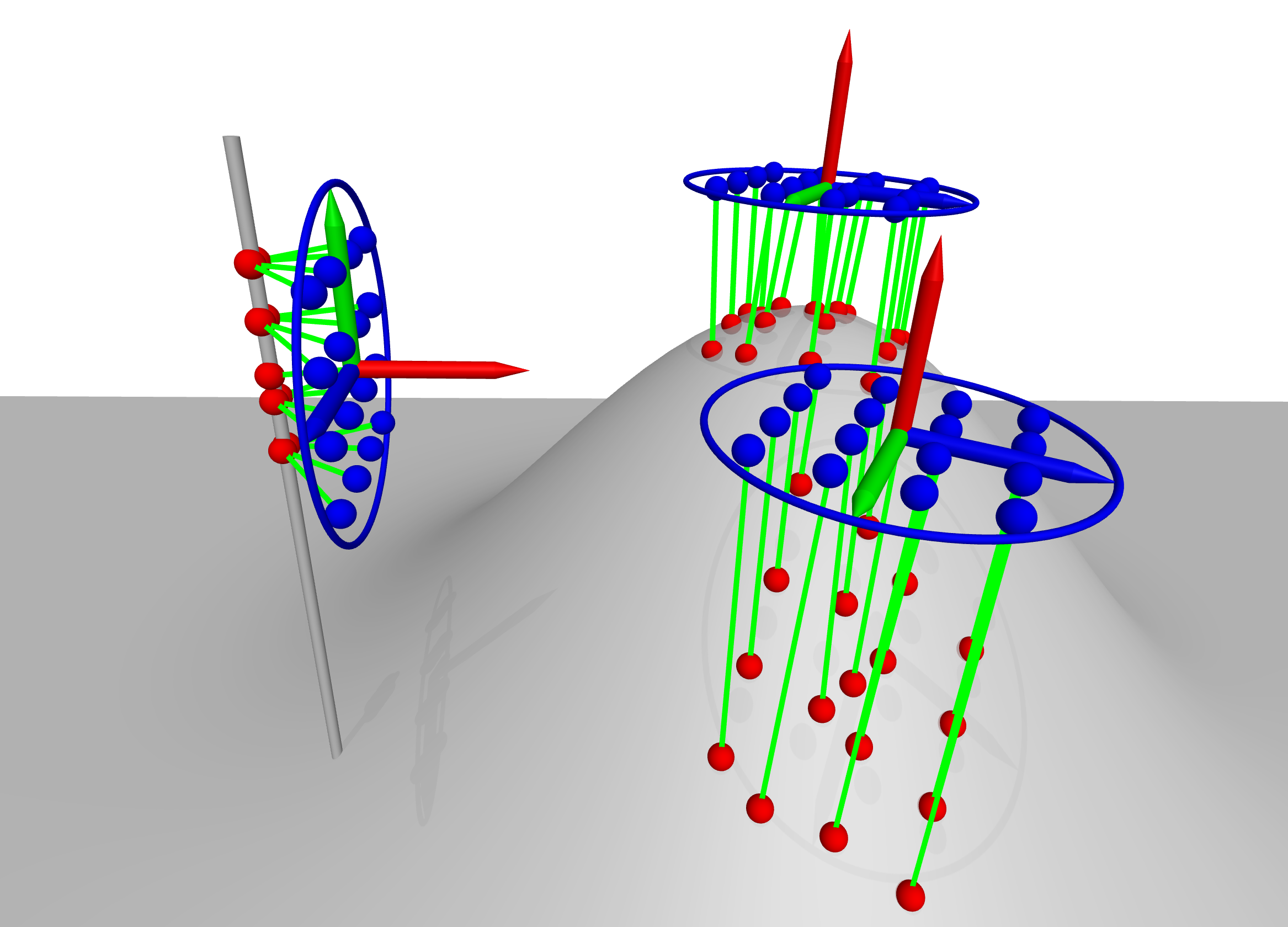
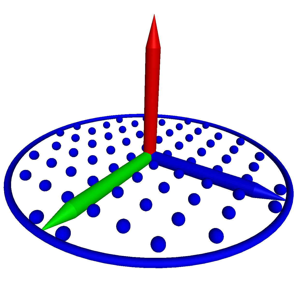
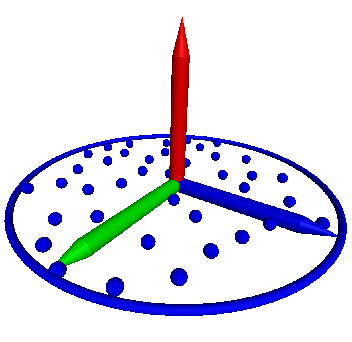
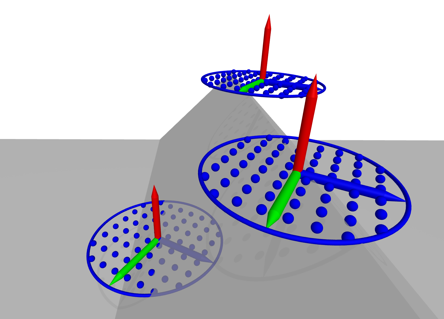
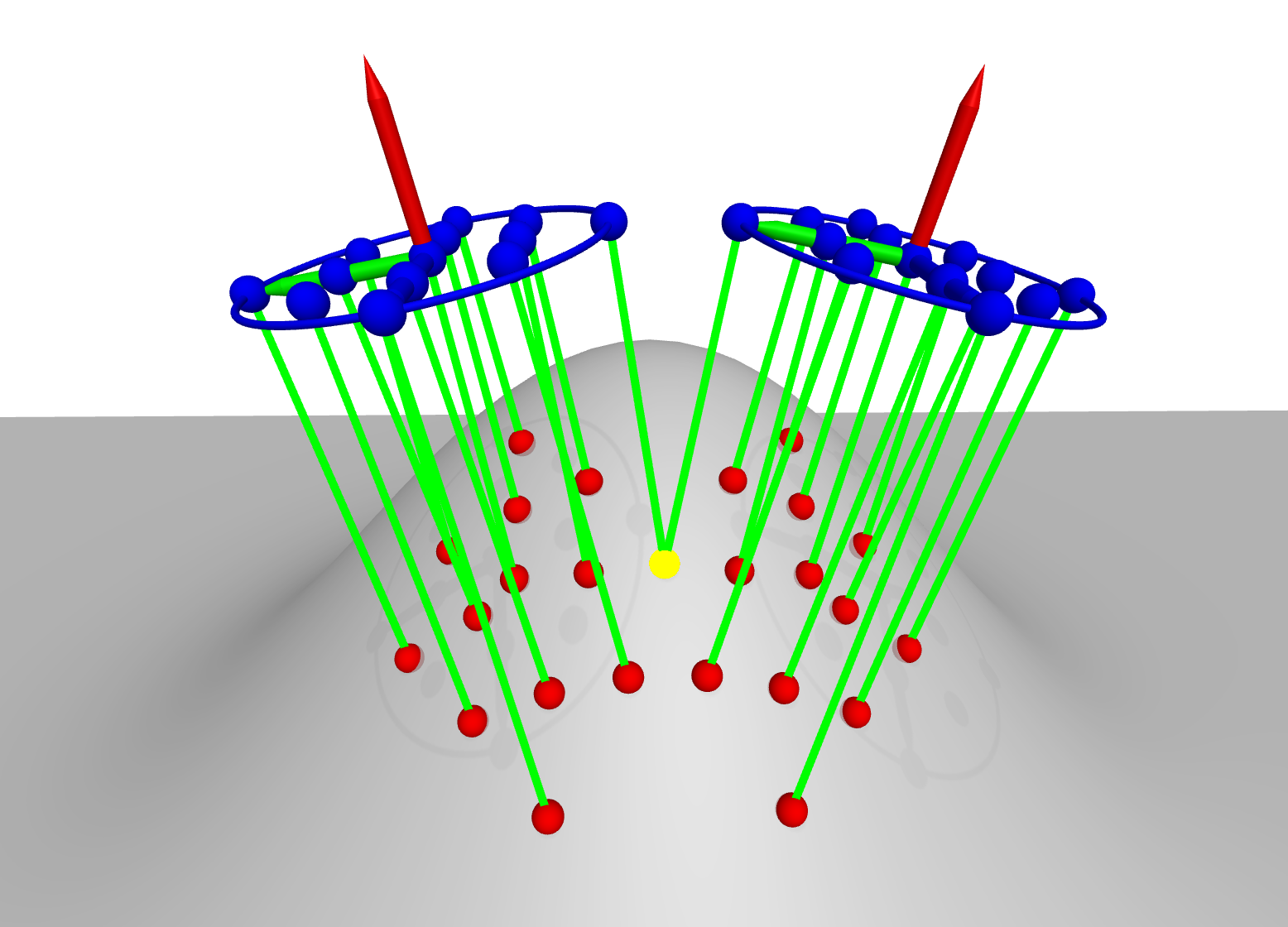
The principal ingredient for building a is a Probing Operator . In its most general form, it is defined as an operator that, to each point in the ambient space assigns a point of the shape near . We will see in next section how a specific probing operator can be designed. A also requires a sampling pattern, a set of points, centered around a seed point and oriented according to an orthogonal frame . It can be made of points sampled on a surface, as shown on figure 3. These points are expressed as offset vectors from the seed to the points. There is no strong constraint on the dimensionality of the pattern, even if it seems reasonable to choose a dimension at least equal to the largest dimension of the input structures. Moreover, the pattern is also free from any regularity contraint. Finally, each accounts for only a part of the shape depending on its initial location. This shape area will be refered to as target area.
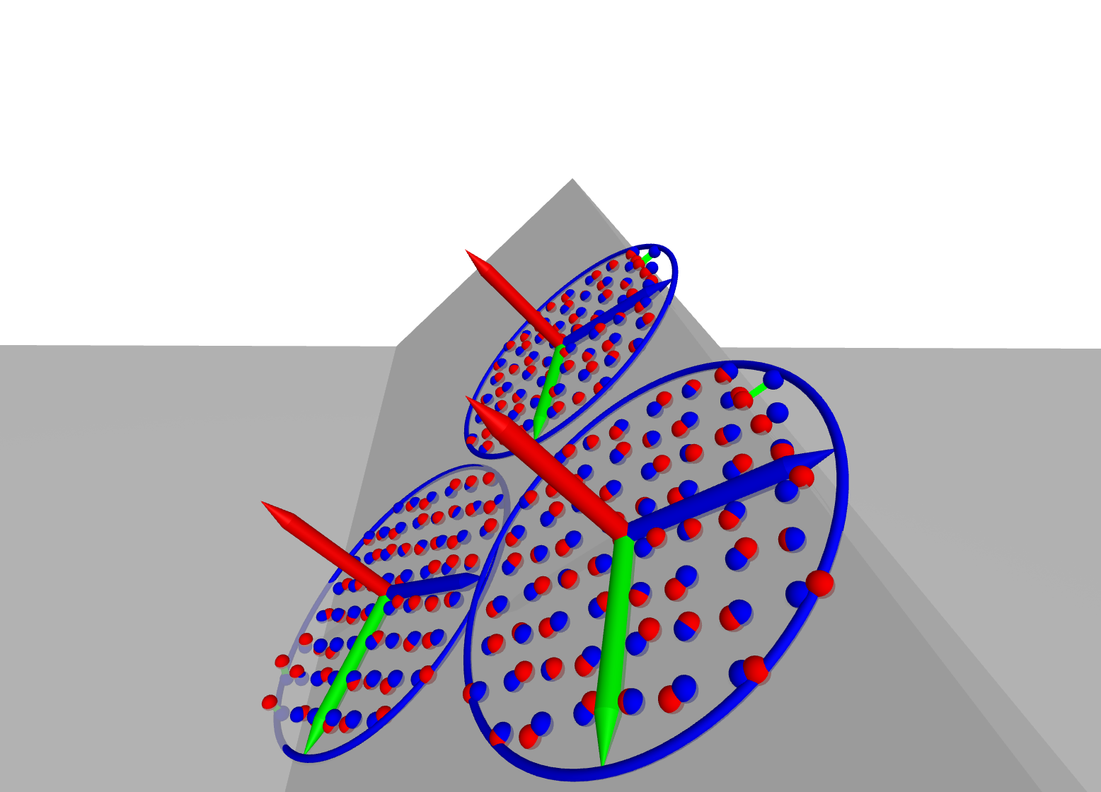
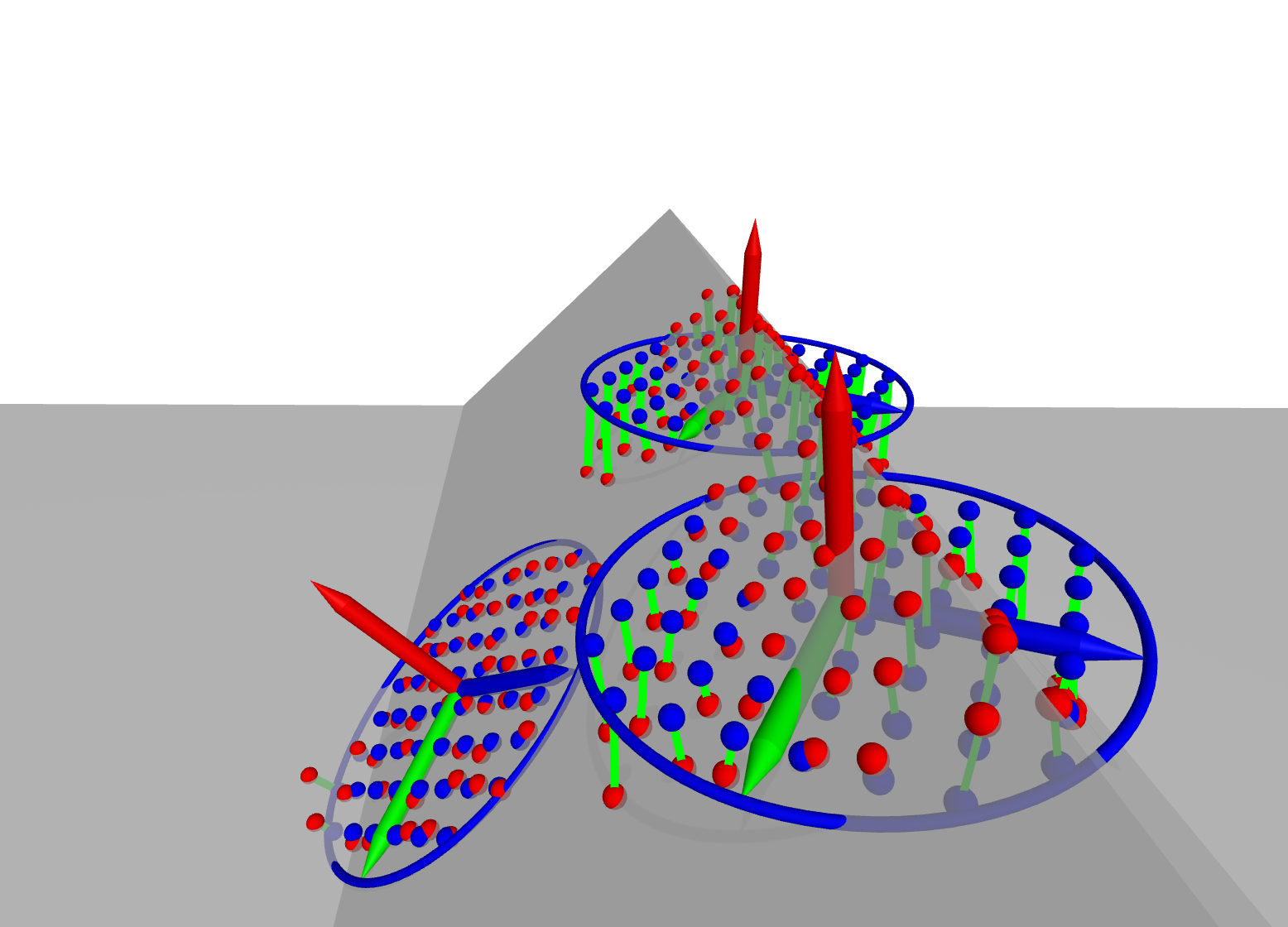
Let us now consider a pattern centered at a point on the shape , and aligned with the local orthogonal frame . Using the probing operator , each point of the pattern is assigned to a point of the target area. Then, the Local Probing Field centered at is the displacement of each point of the pattern to its image under . Let us define:
| (1) |
where is a vector such that . Hence, a is a vector field encoding the deformation of the pattern points onto the shape, without any smoothness requirement or model for the deformation field. Thus, instead of having a prior model, we will encode the shape as a set of local transformations and solely work on these.
2.2 As-Orthogonal-As-Possible LPFs
Given a pattern and a local probing operator, a is entirely determined by its orientation and position. The challenge is to ensure that the resulting representation is efficient enough for the further joint analysis to reveal the shape similarities.
In the case of manifold surfaces, height maps come to mind as a natural and efficient way to represent local surface variations, as height maps contain only geometric information. In our far more general case, we cannot assume that the shape is a manifold, since we want to infer its dimensionality by the learning process. Ideally the should be similar to a height map near a locally manifold surface, but should also handle other cases such as boundaries and curves. Therefore we propose to render the as-close-as-possible to a height map, by maximizing the orthogonality of the vectors with respect to the pattern support plane . Intuitively, when the surface is manifold, the plane parameterized by should be close to the regression plane. With this goal in mind, several probing operators can be devised, depending on the input description of the shape. One can use a simple orthogonal projection on the nearest triangle if the shape is represented by a triangular mesh or a Newton-Raphson projection operator if the shape is represented by an implicit function. In case of point sets, the possible projections range from nearest point projection to variants of the Moving Least Squares (e.g. [37][40]).
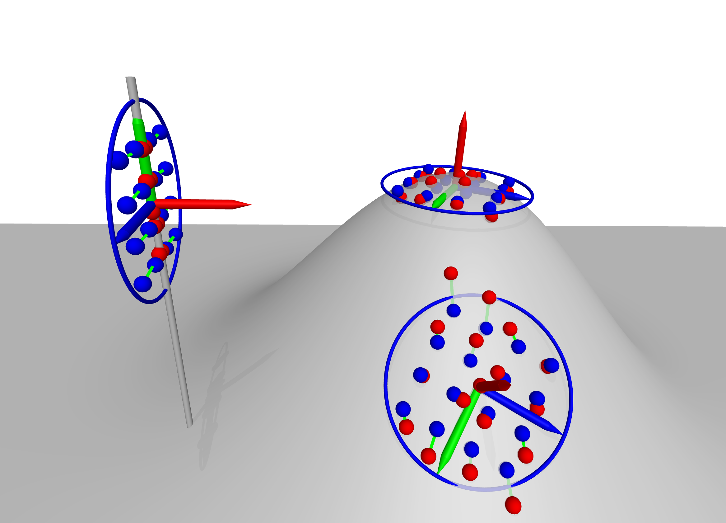
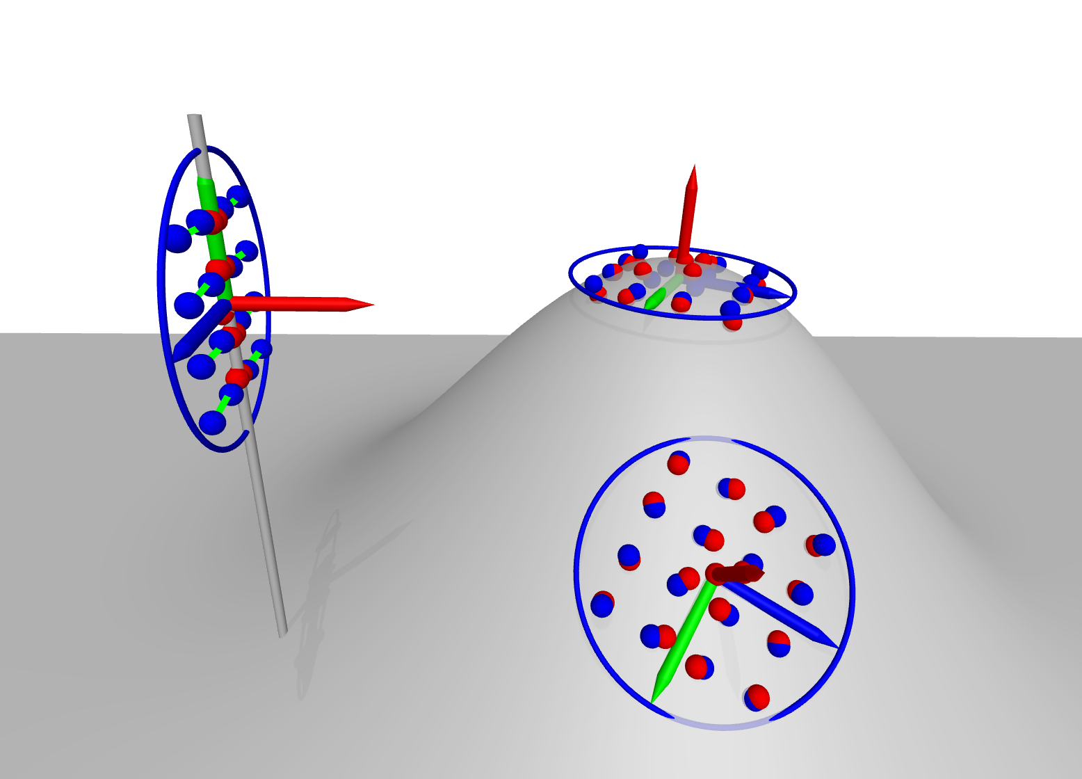
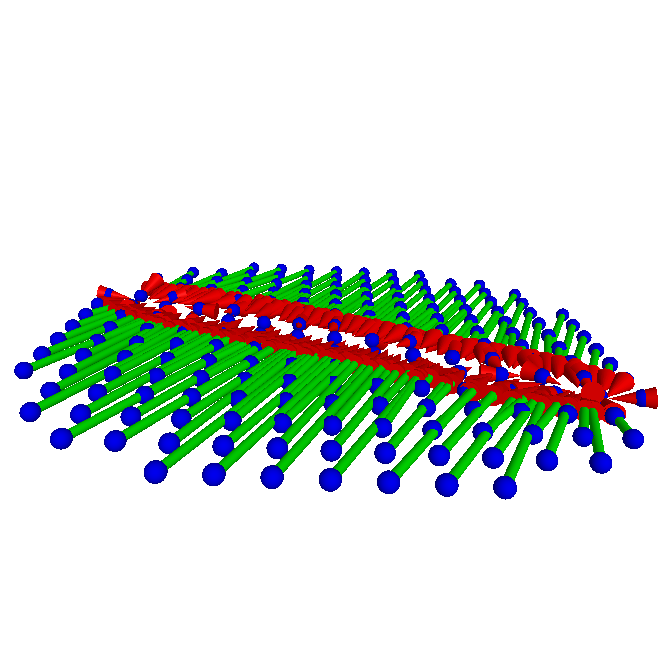
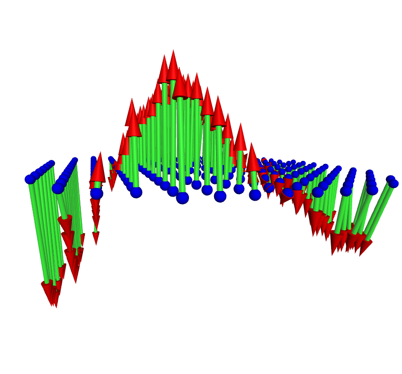
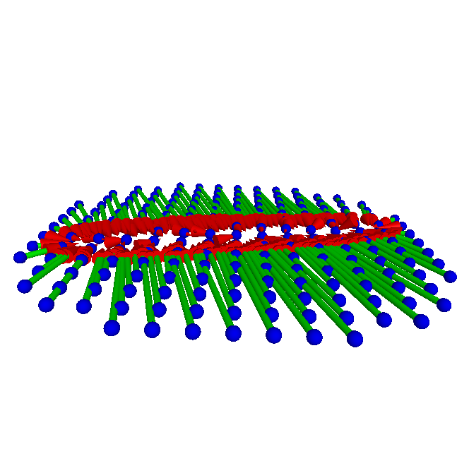
We use a different probing operator aiming at creating as-orthogonal-as-possible s: each point of the pattern is assigned to the point of the target area whose projection on the pattern plane is the closest to . As shown on figure 2, this probing operator captures well both curves (as would a nearest point projector) and manifold surface parts (as would a height map computation).
Moreover, s are generically defined with an arbitrary orientation. We can then optimize each position and orientation to better fit its target area. Unfortunately, using s orthogonality as the sole criterion during this optimization would result in an ill-defined problem. Therefore we propose to minimize instead the norms of the s and alternate the two following steps for each independently:
-
•
Compute . Due to our choice of , s are close to orthogonal to the pattern.
-
•
Find the rotation and translation of the local frame and pattern minimizing the squared norms of the s: .
If the chosen probing operator is the nearest point projector, then the method described above is the well known Iterative Closest Point (ICP) registration [48] between the pattern and the shape. Using the as-orthogonal-as-possible probing operator yields a variant of ICP. An interesting side effect of this approach is that, after optimization, s remain close to their initial target area, whether they are located on geometric features or not. On the other hand, nearest-neighbor-based optimization tends to move s away from sharp features, as shown in figure 4.
3 LPF-based Shape Analysis
Local Probing Fields capture local variations of the shape. These variations can be geometrical and topological. If the set of s covers the whole shape, it is possible to analyze them jointly and thus learn the shape similarities. This joint learning process is partially based on dictionary learning. Describing the shape in the space of deformation fields, changes de facto the space where the shape analysis is performed.
3.1 Initial LPF positions
A set of s is built at arbitrary locations around the shape, with arbitrary frame orientation. The only constraint on this initial set is that the set of target areas should provide a possibly overlapping covering of the shape. For example, a pattern can be initially positioned on a sampling of the shape (e.g. each vertex in the case of a mesh or a point set) with a random orientation. They can also be aligned with principal directions if they are defined, which is not the case for curves. To illustrate the efficiency of our framework, we distribute s on the shape using a Poisson sampling process and use random initial orientation. These positions and orientations are further improved using the minimization defined in section 2.2.
In practice, the target area of a given is set as the intersection of a sphere centered at with the shape. The radius of this sphere is set to be slightly larger than the pattern radius in order to relax the position of the LPF with respect to the target area while still ensuring that the information is well represented. In our experiments, we chose . With this definition, s should be located near the shape to have non-empty target areas. As a consequence, although positions and orientations of the s evolve during the analysis, the target area of each remains unchanged.
Let us notice that if the sampling density of the pattern is below the sampling density of the shape, the representation is conservative. In that case, the shape can be exactly reconstructed from its set of s.
3.2 Joint Analysis Overview
Our shape analysis process computes:
-
•
A dictionary of atoms that best describes the s, and therefore the shape.
-
•
A sparse set of coefficients to decompose each on the dictionary. The sparsity constraint enforces a consolidation of the information.
-
•
positions and orientations that best enforce a consistent representation, their target areas being fixed.
Let be the total number of s. Writing the s as vectors , , the problem can be stated as follows:
| (2) | ||||
Previous works on sparsity have mostly focused on minimizing the representation error: given a set of signals , the aim is to find the best dictionary to represent the set of signals in a sparse manner (few non-zero coefficients). In our approach, we tackle a more complex problem since both the signals and their representations are optimized while subject to very strict constraints. The dictionary learned on the initial set of s is strongly dependent on initial positions and orientations of the patterns. As a consequence, two similar parts of the shape might be described by non-similar s because of different initial poses, whereas their difference could be reduced after a change in position and orientation. The goal of the energy minimization is thus to improve dictionary learning via enhancement of the s similarity.
Our algorithm iterates the following steps:
-
1.
Dictionary learning: Solve for minimizing .
-
2.
Pose optimization: For each , solve for the translation and rotation minimizing the representation error and update the , seed and frames accordingly.
-
3.
Update: Update each using the probing operator.
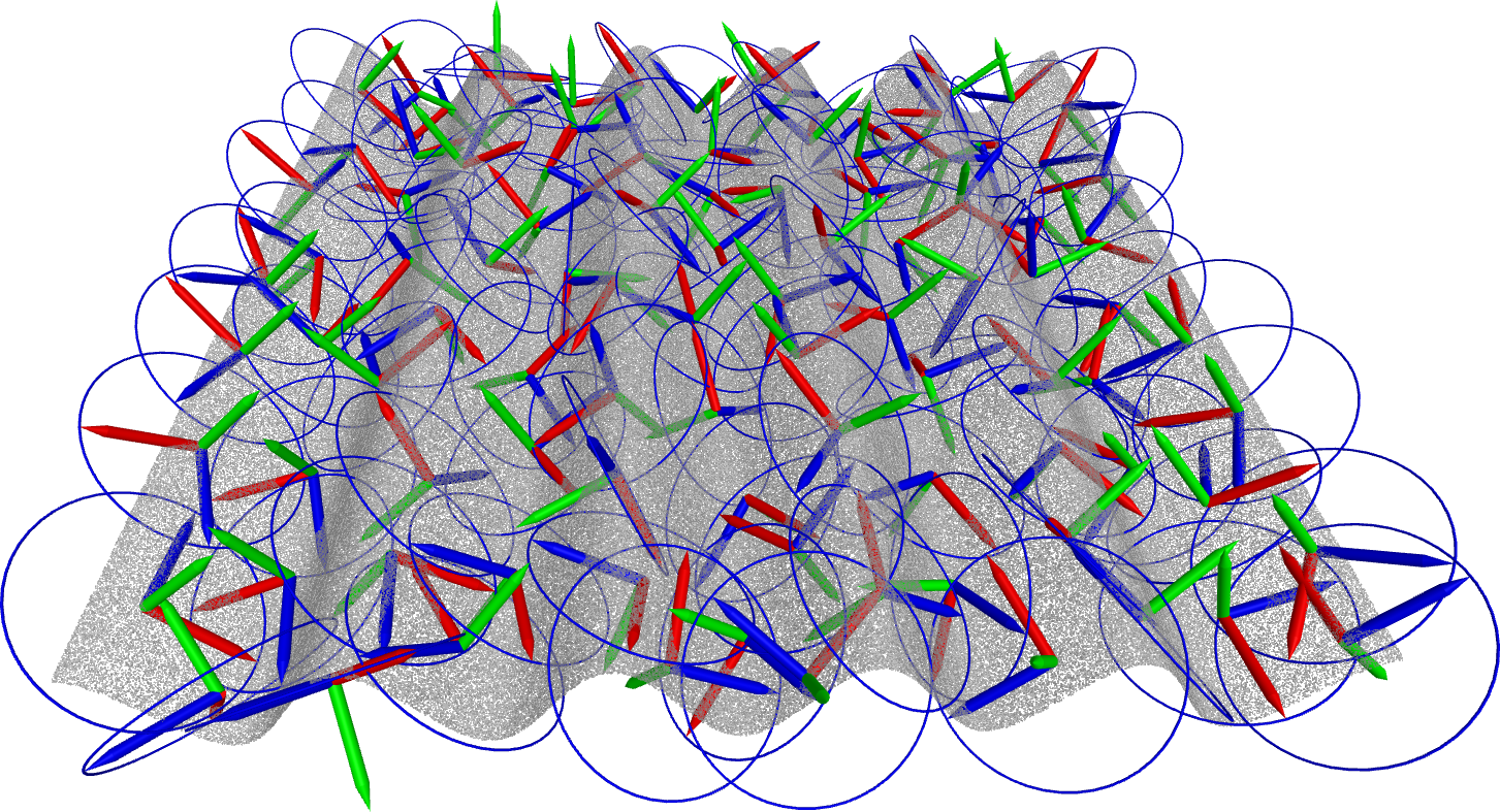
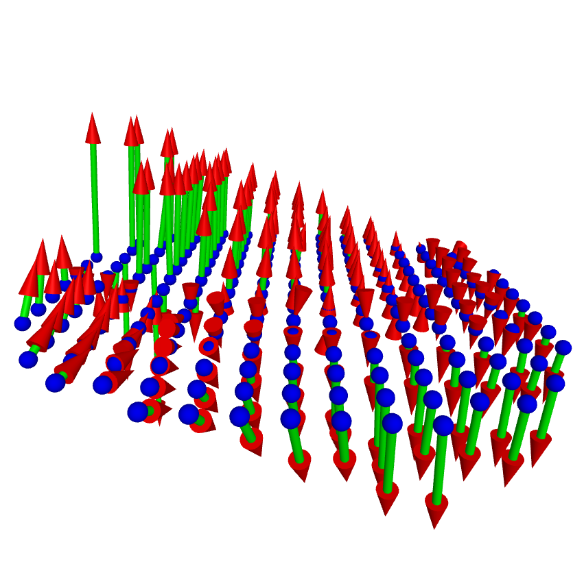
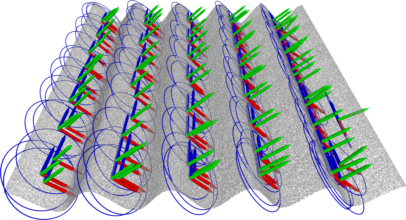
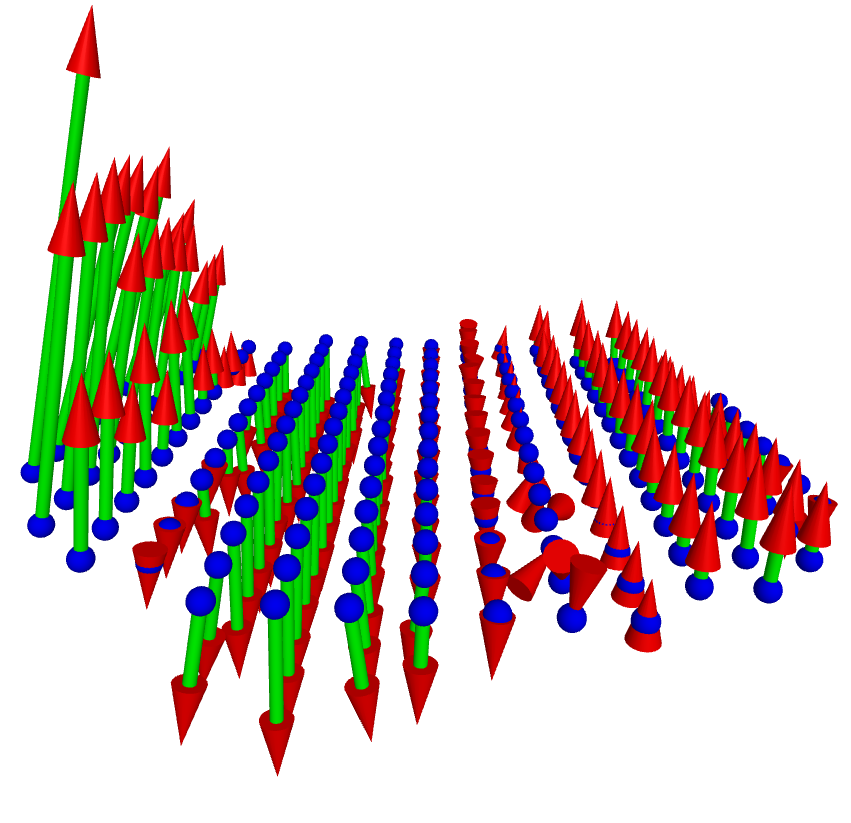
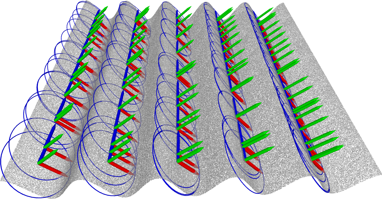
Figure 5 shows how our algorithm captures the self-similarities of a synthetic shape. Starting with points sampled randomly on a sinusoidal surface, we set initial s with random position and orientation on the shape. We then iterate our joint analysis method. The result shows that the s align at positions that represent similar parts of the shape, and their optimized orientations are consistent.
3.3 Sparse Coding For Dictionary learning
The first optimization aims at learning a good dictionary over which the signals will be sparsely decomposed. Let us write the s as vectors for . Then the representation optimization corresponds to the Least Absolute Shrinkage and Selection Operator (LASSO) problem, which is defined as the minimization of:
| (3) |
with and . As stated in [12] and [49], the norm is empirically known to provide sparse solutions while improving the speed of dictionary learning compared to the so-called norm (number of non-zero elements in a matrix). The dictionary is initialized with elements drawn randomly from the set . Afterwards, the algorithm alternates between the two following steps:
-
•
Sparse coding step to compute , , using the Least Angle Regression (LARS) algorithm [50].
-
•
Dictionary update step, performed by using the previous dictionary as a warm restart to minimize the objective function.
The steps are iterated until convergence of the representation error is reached. In our setting, iterations are sufficient for the error to converge. The parameter controls the sparsity of the solution: large values will favor very sparse solutions while small values will yield dense solutions. In our tests, we set for dictionaries with a large number of atoms, and for small dictionaries, to allow enough non-zero coefficients for shape representation.
The dictionary is initialized to a random subset of the LPFs. Since our algorithm converges to a local minimum, a different random initialization might lead to different minima. We experimentally observed the stability with respect to the random dictionary initialization, by running the shape analysis algorithm times with the exact same parameters, starting with a different initial random dictionary and measuring the representation error (3) divided by . This experiment yielded an average error of and a standard deviation of , thus showing that our algorithm is rather stable to the random dictionary initialization. Although the error converges to similar values, LPF Analysis is unfortunately not guaranteed to converge towards the same dictionary given different initializations (similarly to K-Means or K-SVD). A stable dictionary would be of great interest for applications such as shape matching and retrieval. However, for the applications shown in this paper (resampling and denoising), stability of the dictionary is not crucial, since it is an intermediate representation and not the output of the algorithm.
An alternative for the sparse coding step might be to use Deep Learning and especially auto-encoders but the optimization of position and rotation to ensure that LPF representation of similar regions are indeed similar does not write in a simple way.
3.4 Pattern pose optimization
The previous sparse decomposition steps introduce a representation error. But reducing this error is still possible by improving each pose individually, to find the optimal fit between the shape and each newly modified . This can easily be done using a least squares minimization step, similar to what is done during one ICP iteration. More precisely, one looks for a translation of the and a rotation of its frame such that the newly defined vectors fit better the ones obtained by dictionary decomposition . After a rotation of the frame and translation of its position, the modified can be expressed as:
| (4) |
The best rotation and translation thus minimize:
| (5) |
which is exactly a least squares minimization for estimating a rigid transform between two sets of points: and .
Using these optimal rotation and translation for each , the seed position , frame orientation and vectors should be updated accordingly:
| (6) | ||||
This update maintains the consistency between the shape and the description, position and orientation of the s.
3.5 Closing the loop
After the pose optimization step, the set of optimized s is better suited for the input shape analysis. We use once again the probing operator to probe the shape with respect to the optimized pose. To avoid s gliding on the shape (with the risk of losing the shape covering), we restrict the update to its original target area. Therefore, although each pose and sparse decomposition is optimized, it always accounts for the same shape area. This update can theoretically increase the error but we observed experimentally that the error decreases across the iterations (see Fig. 6). Then, we are able to repeat all the processing steps until convergence is reached. Figure 6 shows the evolution of the error with varying dictionary sizes on the Brassempouy point set.
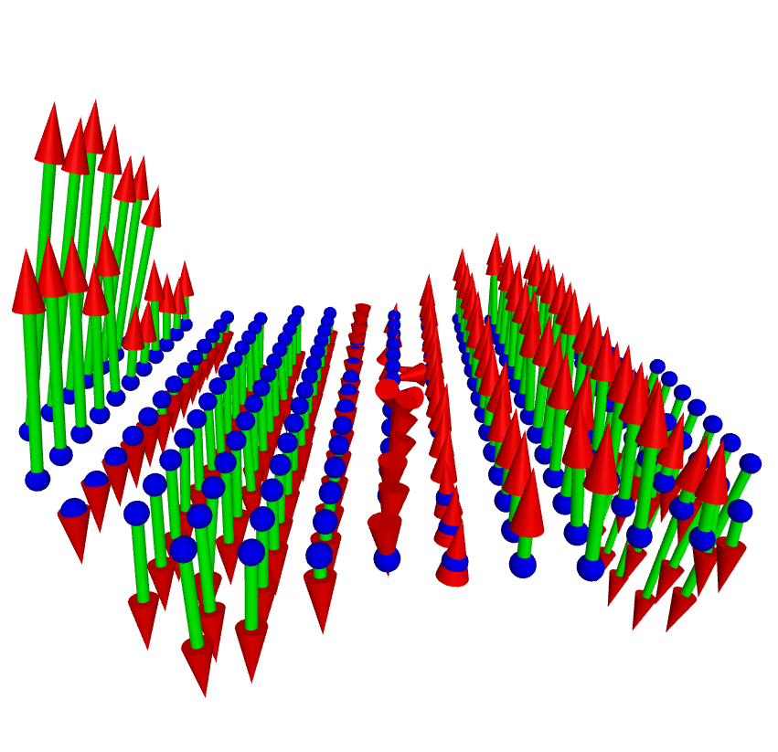
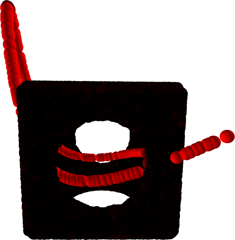
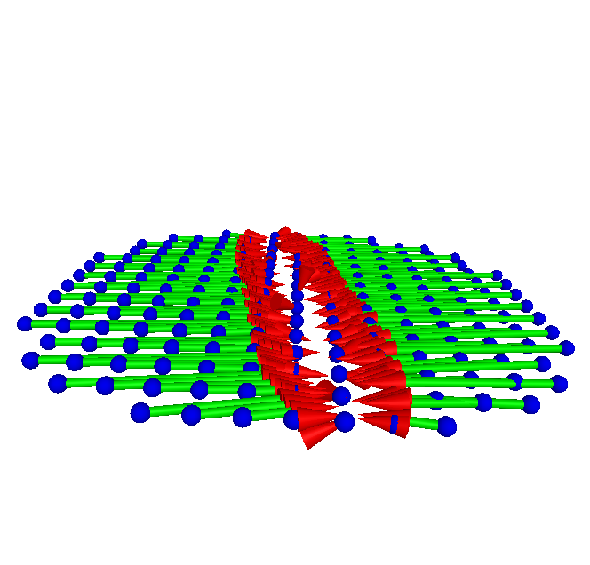
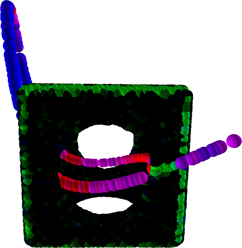
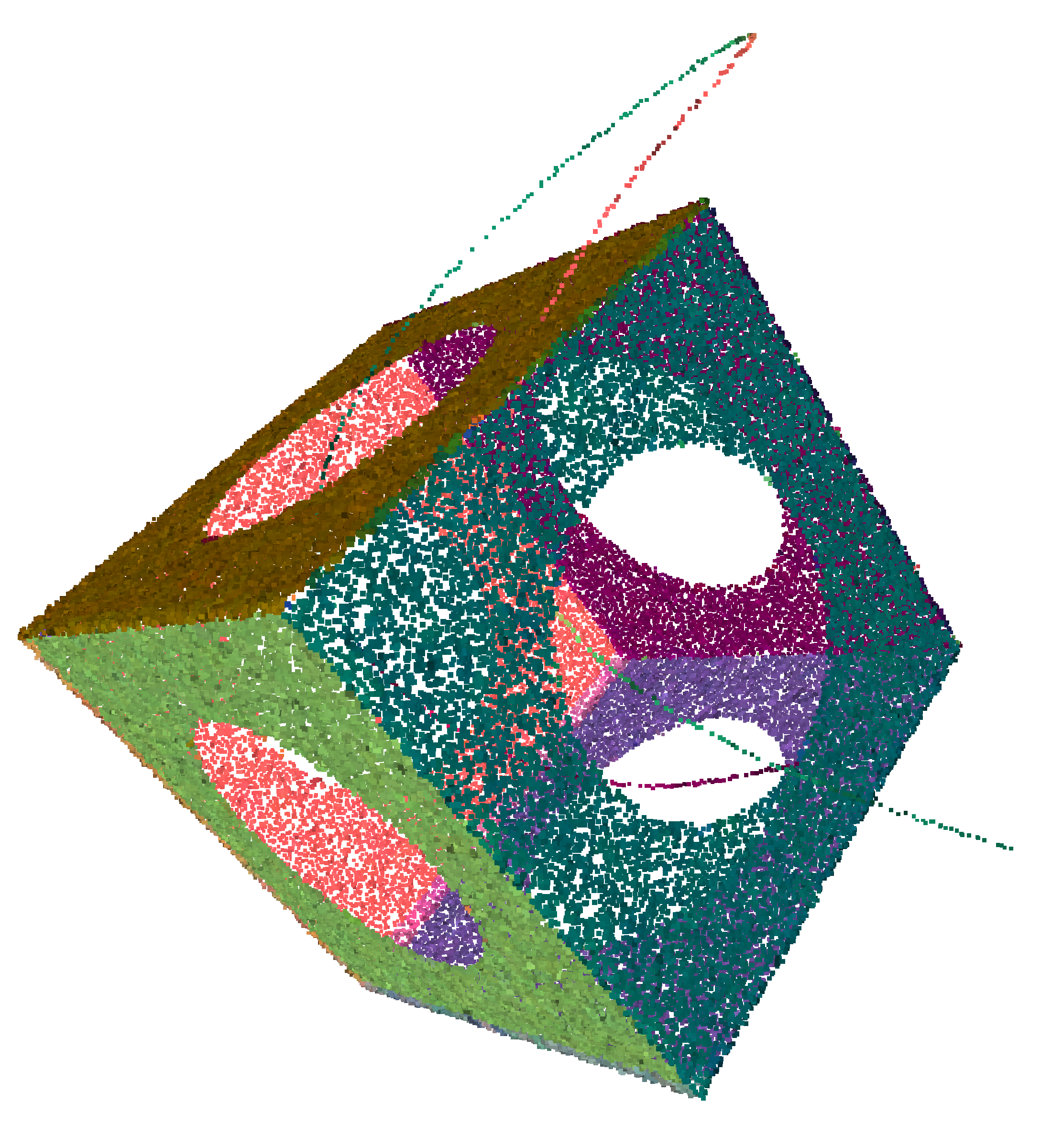
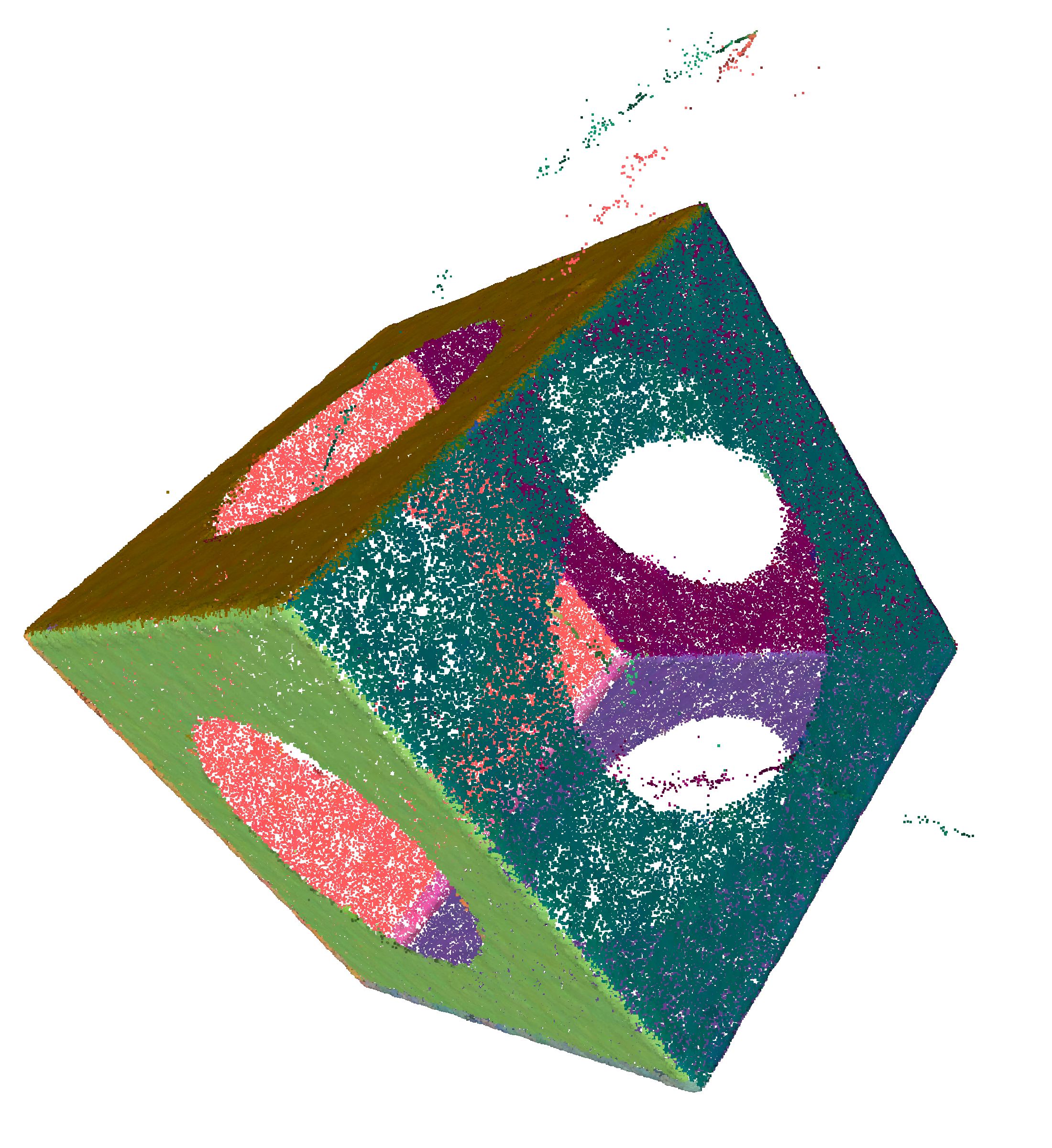
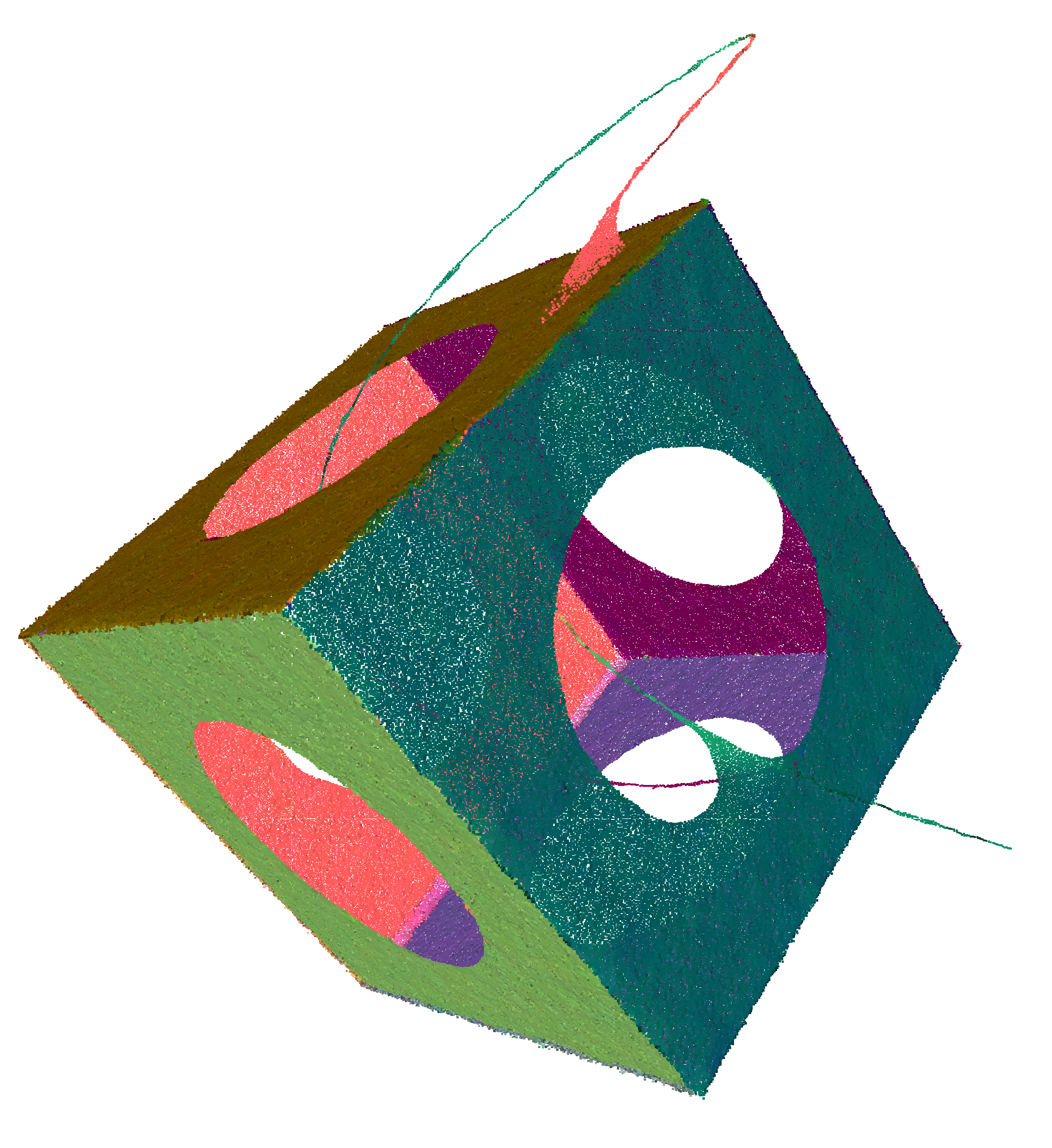
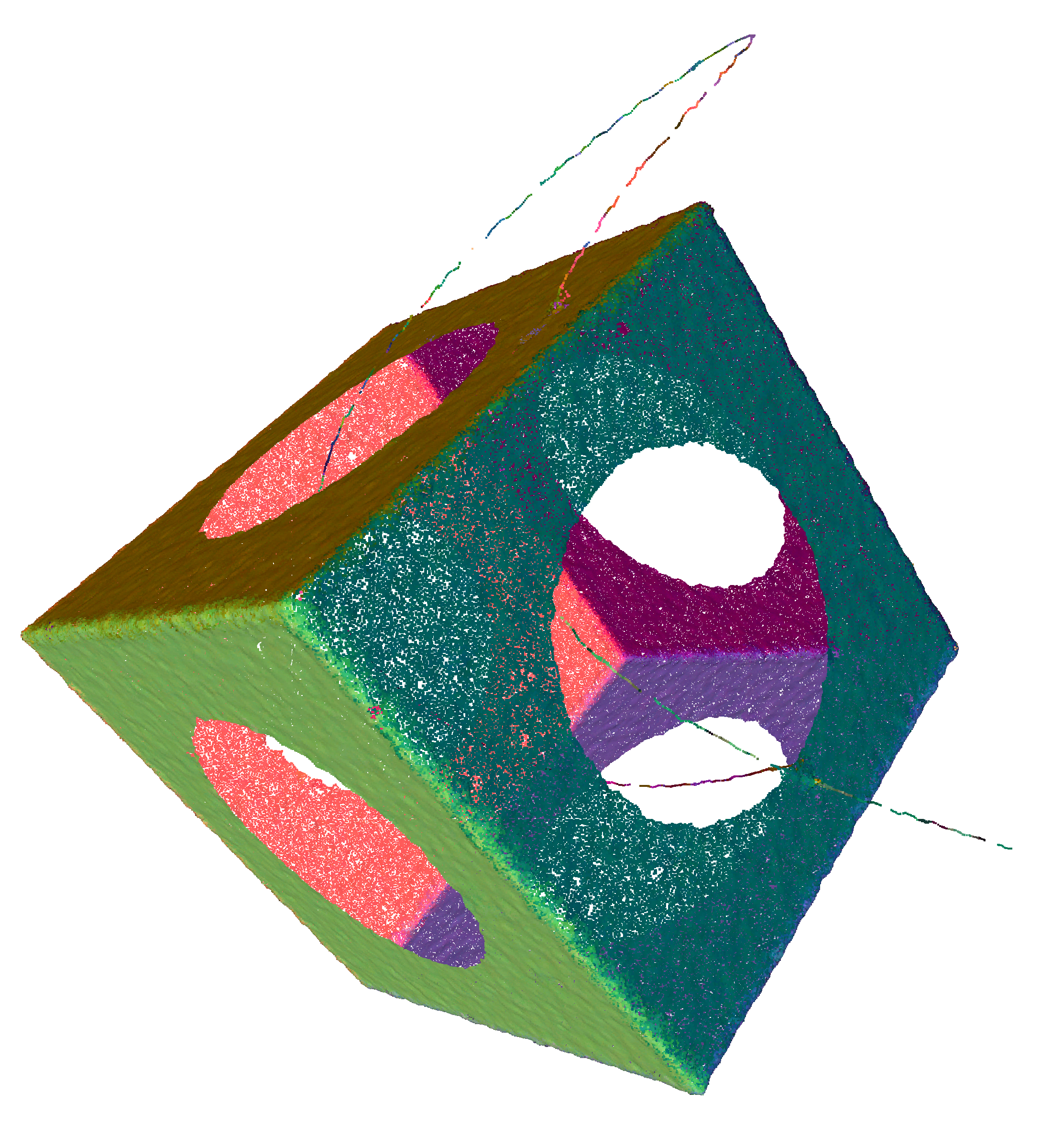
Figure 7 shows the analysis result for a shape representing a cube with a curve when using a dictionary of size and . When using 1 atom, the decomposition (a) mostly encodes the curve, while sharp features are undetected. When using 3 atoms, the decomposition (c) exhibits significant coefficients on sharp edges or on the curve. For both cases, the remaining parts of the shape are represented with small coefficients for all atoms. (b), (d), (e) and (f) show atoms representing sharp features and curves. These experiments show that the final dictionary retrieves important features of the shape.
3.6 Controlling the shape analysis
Our shape analysis approach is driven by three parameters: the pattern radius , the number of points of the pattern, and the number of dictionary atoms .
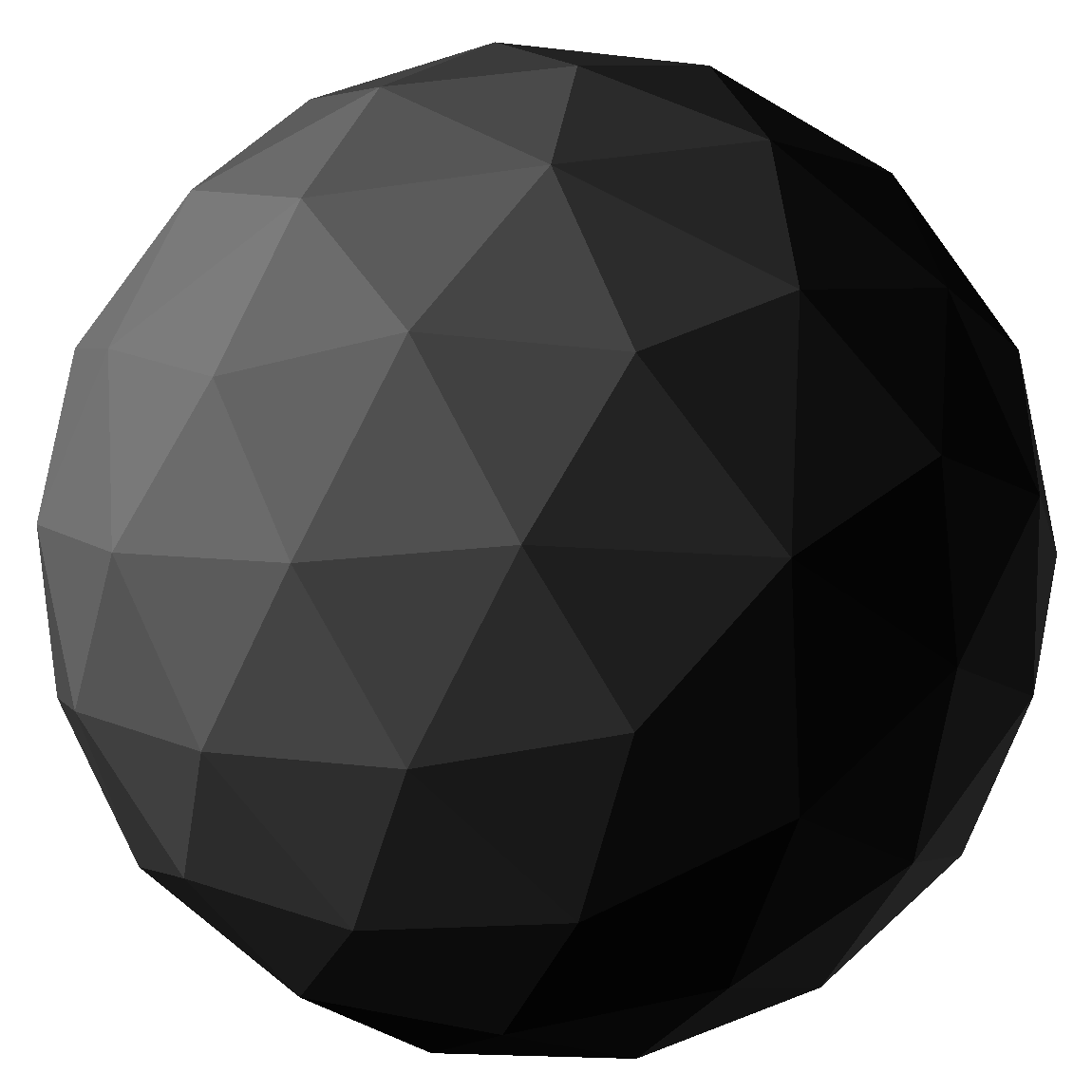
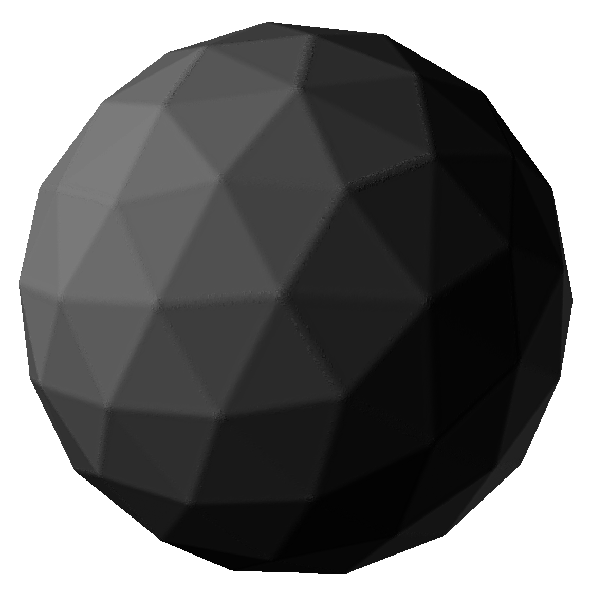
The pattern radius is linked to the shape geometry: it represents the scale at which the similarities can be exploited to build the dictionary. On Figure 10, we illustrate the importance of the radius: with a large radius, the faceted sphere mesh is interpreted as a sphere, whereas it stays a piecewise linear shape with a small radius.
Once is fixed, the number of points in each pattern controls the accuracy of the analysis. This accuracy can be measured by the average distance between pattern points. Assuming that the points are uniformly sampled on a disk of radius , each point represents a region of area . Thus, an estimation of the distance between points is . Hence, once is fixed, can be computed as: . can then be adjusted at will, to perform different sampling scenarios, depending on the input shape: if the probing operator accuracy is , setting will perform a sampling scheme. Setting will double the number of sampling points, as shown on figure 1. In practice, an efficient way of building a pattern is to generate a regular grid with a step of size and keep only the points that are included within a radius .
The number of atoms controls the amount of consolidation. If the number of s is equal to the number of atoms, then no learning is performed since all s can be represented independently, and there is no consolidation. Conversely, fewer dictionary atoms implies a stronger consolidation. Therefore the number of atoms in the dictionary controls the degrees of freedom in the representation, i.e. the supposed variability of local parts of the shape. can be increased until the error falls under a threshold that is consistent with the accuracy of the probing operator. Interestingly, when the sampling pattern is planar, all dictionaries naturally allow to represent planar regions as any atom multiplied by results in a planar shape.
Finally, let us notice that the analysis framework is entirely driven by the minimization of Equation (2). First, the dictionary learning minimizes the error with fixed LPFs. Then, the pose estimation step keeps the dictionary and coefficients fixed and minimizes the error by aligning the s to match the dictionary decomposition, therefore, the component remains unchanged while the component decreases making the sum of the two components decrease.
The last recomputation step is not guaranteed to reduce the error, since the probing operator is used once again to recompute the s. Without this step, the error defined by Equation (2) would always decrease and convergence would be guaranteed. In our experiments, we observed that in most cases, this recomputation step made the error decrease. However, in a few cases the error increased marginally but that was compensated by the decrease in the two other steps. Moreover, using the recomputation step yields lower errors and better dictionaries.
4 Applications
4.1 Shape Resampling
The shape analysis of section 3 provides us with optimized positions and orientations as well as a shape dictionary and the associated decomposition coefficients . We propose to use these optimized s to sample points on the shape.
First, the vector fields are recomputed using their decompositions . Each yields a set of points such that:
| (7) |
where are the coordinates of vector (and similarly for ). Since the s overlap, the reconstructed information in the overlapping areas may not coincide exactly. In these areas, a consensus point distribution, still driven by the error minimization, must be built. Let us call an hypothetical best consensus position. This point is located inside the target areas of several s. A point of a reconstructed is said to conflict with a point if the target area of includes and . In practice this means that the yields a point close to . Let us define the influence zone of as the set of conflicting points. A consensus point should minimize:
| (8) |
This minimization is non-trivial since varies with . Fortunately, we can simplify it by fixing the set which yields a least squares minimization resulting in: . In practice this means that when a proposes a position , the best consensus point is found inside , and is moved at this optimal position. Afterwards, no point conflicting with can be added to the resampled point cloud.
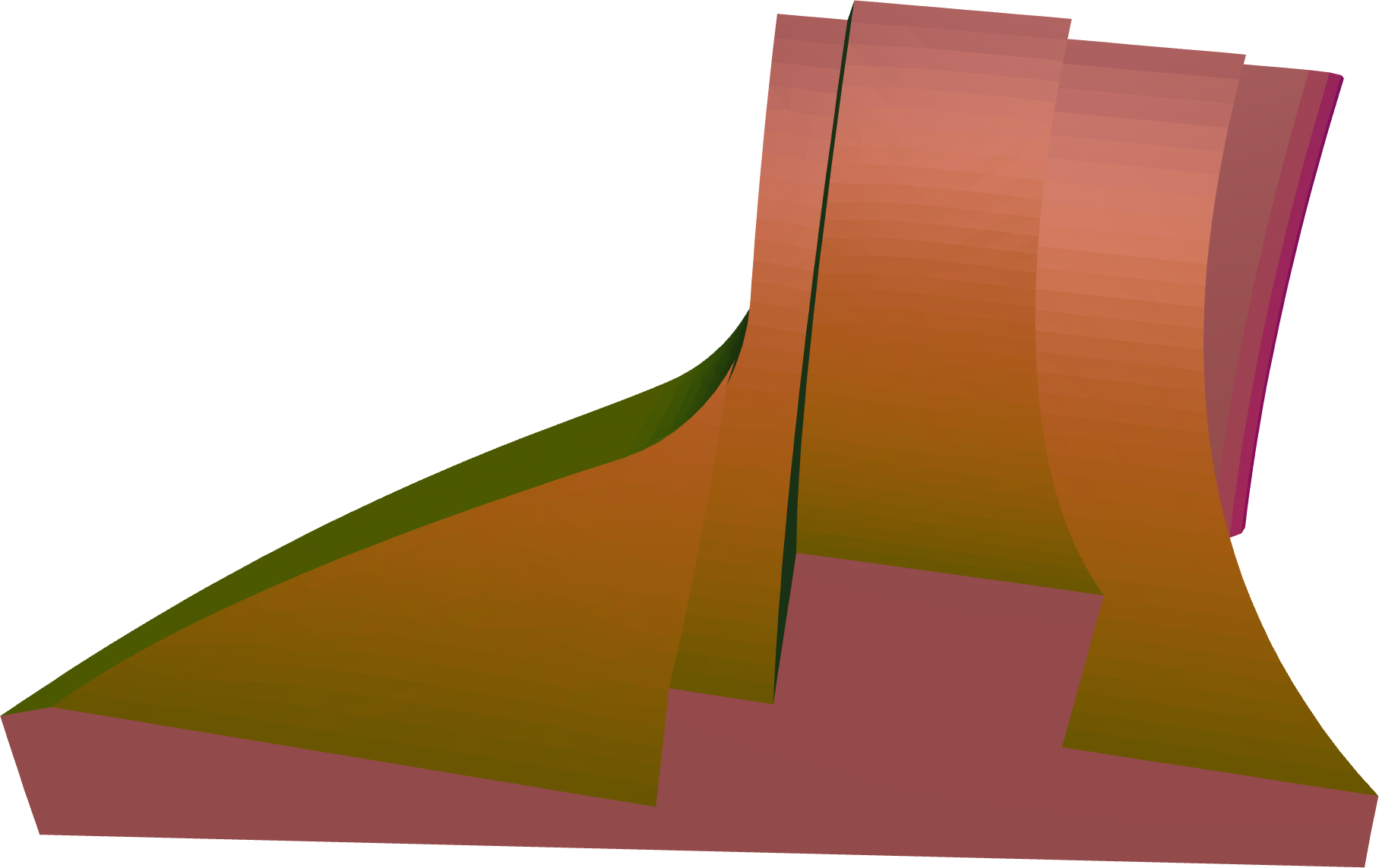
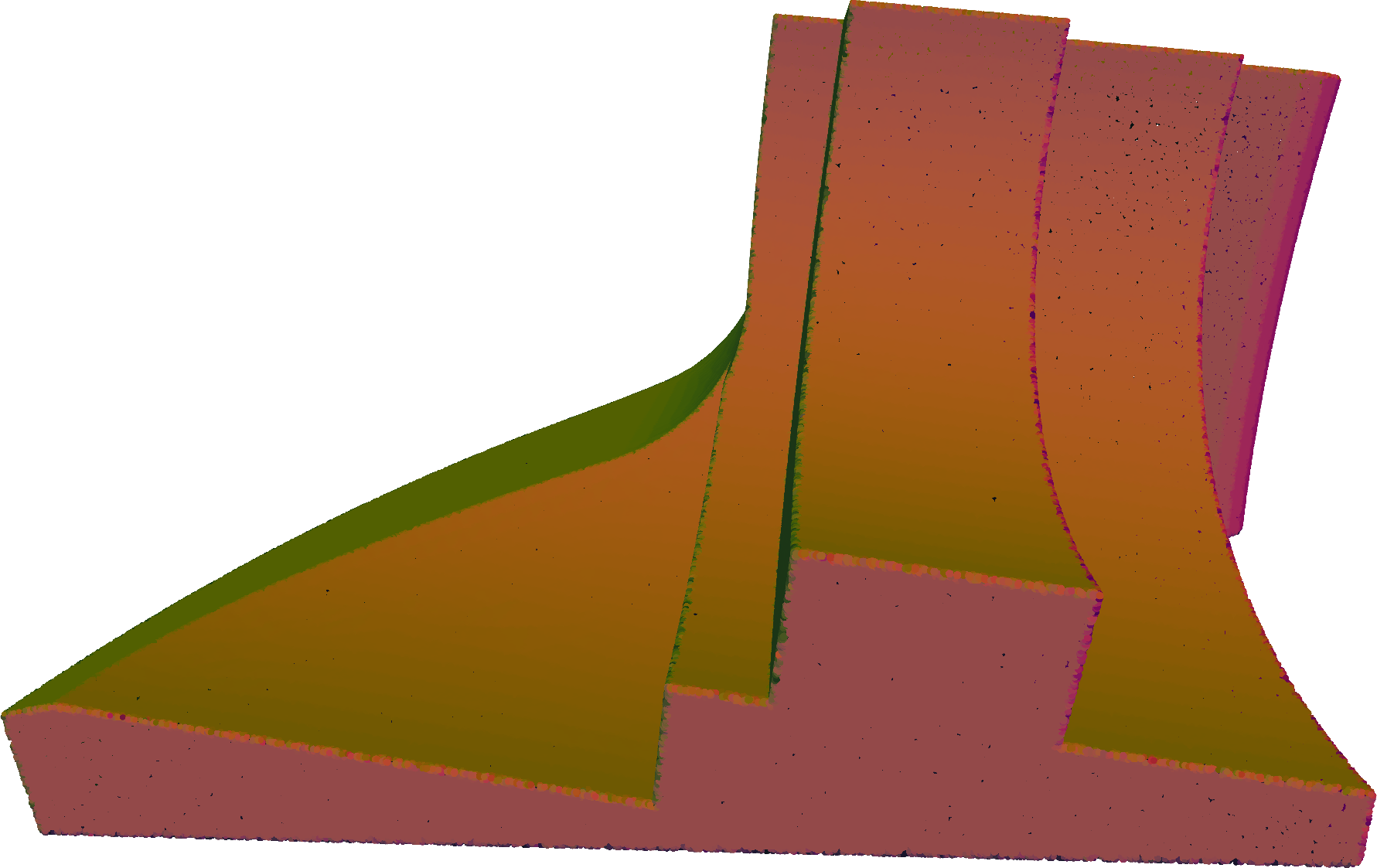
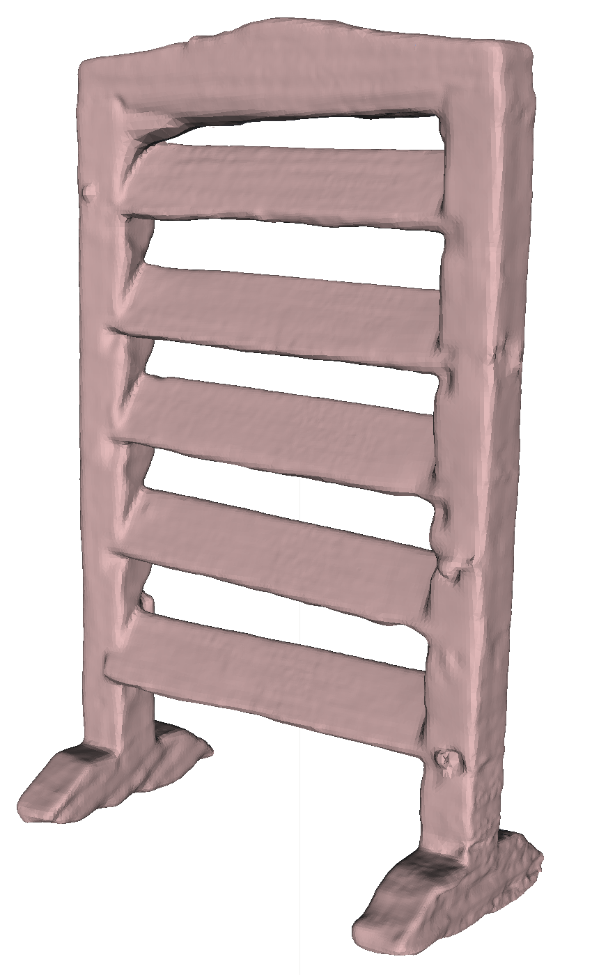
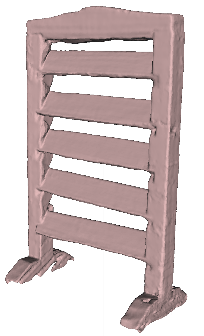
We experimented our framework on shapes represented as surface meshes (Figures 10, 11) and point sets (e.g. Figures 1, 14). On a LiDaR point set (Fig. 12), our framework yields a detail-enhancing resampling which preserves well the point set borders. We first illustrate how the resampling removes the noise in a feature preserving way (Figures 13, 14), in particular for open surfaces. On Fig. 14, we show the result of applying the Screened Poisson Reconstruction [51] after resampling the shutter: the sharp edges and details are much better enhanced.
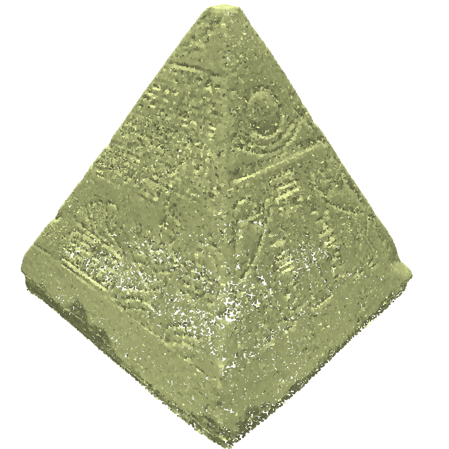
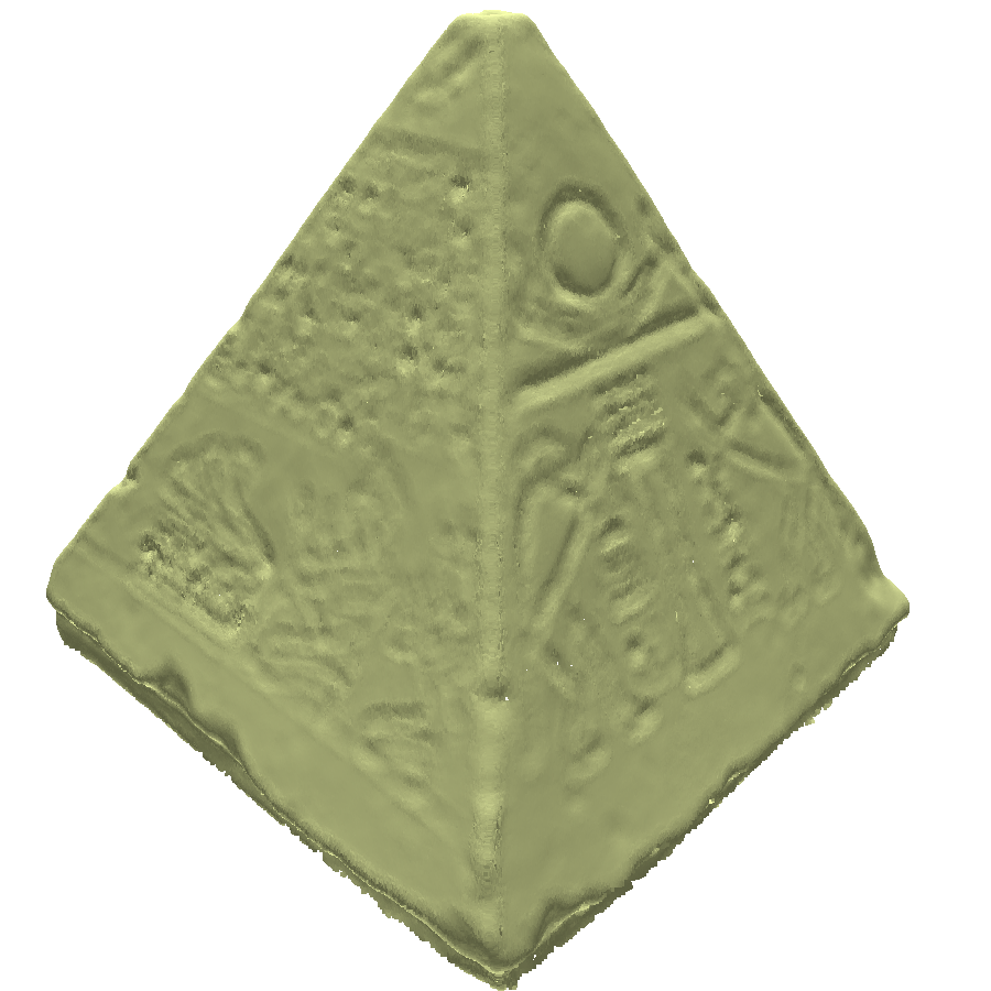
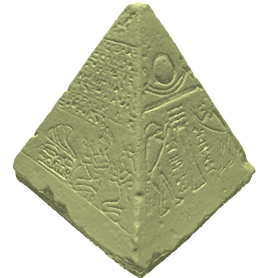
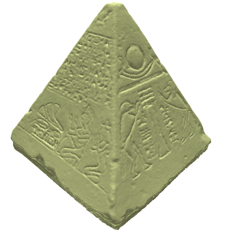
We compare it with EAR [34] on a pyramid shape with engravings (Fig. 15) and sparse initial sampling. EAR and LPF both outperform Moving Least Squares and permit to upsample the shape while recovering the engravings. On the contrary, on the cube with curve model or ship point set, EAR is bound to fail at resampling faithfully the curve because of its manifold surface assumption (Figures 1, 8).
The obtained shape sampling rate is guided by the sampling rate of the pattern. This can experimentally be seen on Fig. 16, where a planar grid is used as pattern. In this experiment of a perfect plane resampling, the mean distance between two points is strongly linked to the distance between two points in the resampling pattern. If the pattern is a grid (thus points once intersected with a sphere) and , the grid step is and the measured mean is . Similarly for a grid and (resp. a grid and ) the grid step is (resp. ) and the measured mean (resp. ). The histograms of the distance to the nearest neighbors are also shown on Fig. 16. These distributions are very close to what Poisson disk sampling would do, which is due to the consolidation process. One can see that the sampling remains stable and the density is driven by the distance between points on the pattern.
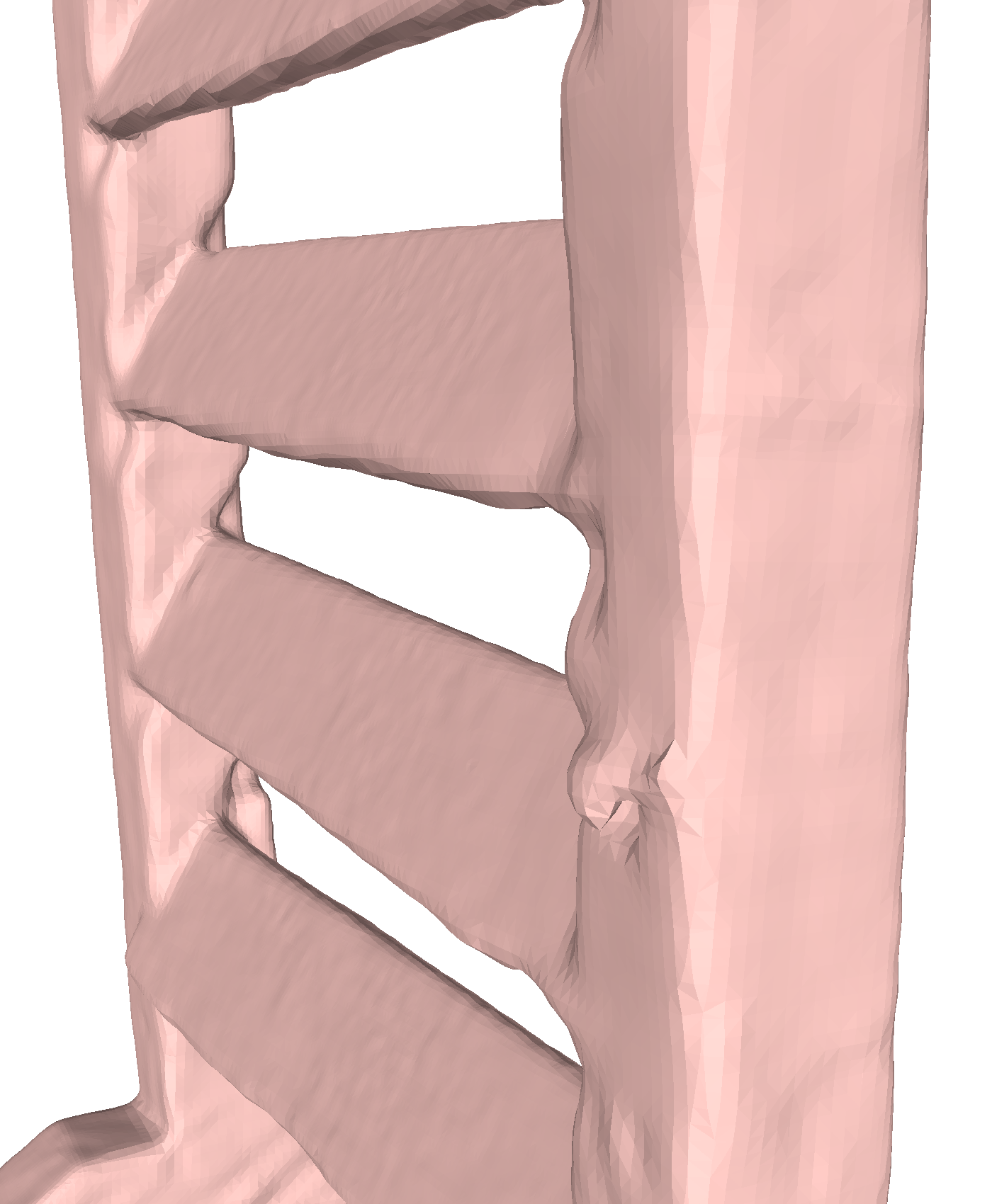
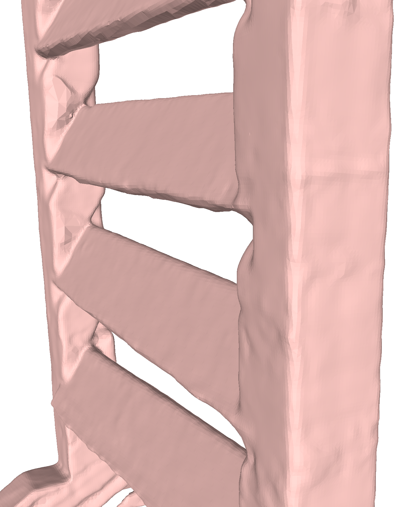
One important feature of our method is its ability to learn the local dimension from the shape, which can be seen on the cube with curve point set (Fig. 8). EAR being particularly well suited for edge recovery, it performs better on the edges of the cube but it fails to recover the curve structure whenever it is too close to the shape. On the contrary, is able to resample it. This advantage of our method can also be seen on the ship example (Fig. 1). We have enhanced the MLS-based resampling with an anisotropic behavior: we measure a local stretch ratio , the ratio between the two largest covariance matrix eigenvalues. In the regions where is below a threshold ( in our case), MLS sampling occurs as expected, while regions where is above the threshold are sampled as curves. This modification improves the sampling of the curves, but it still tends to blur the riggings, and creates spurious points. EAR fills the gaps between the ship’s rigging, whereas nicely enhances them.
4.2 Point Set Denoising
The second application of our framework is point set denoising. Similarly to [53], we start from the initial point set and aim at finding the denoised point set minimizing the following objective function:
| (9) |
where is the operator that extracts the at position (i.e. ) and are two parameters constraining the data attachment and the sparsity. corresponds to the squared distance between the initial noisy point set and the current point set, measured as the sum of squared distances from points in to their nearest neighbor in . This objective function is hard to minimize but is in fact closely linked to our minimization defined in Equation (2). We solve it by splitting it into two steps that are iterated until the point set is stable
-
•
The first step learns the dictionary and coefficients as well as the positions and orientations.
-
•
The second step uses the dictionary to find the best denoised point set.
The first step is exactly our shape analysis defined in Equation (2). Then, once the dictionary and coefficients are fixed, minimizing (9) amounts to solving in the second step:
| (10) |
Minimizing this energy means finding for each point the best consensus among all s that describe the vicinity of . More precisely, each initial point relates to a set of consolidated s providing better candidate positions for this point, i.e. positions that fit better the dictionary decomposition. A better position estimation can thus be computed, similarly to the shape resampling application: starting with an initial point position , each neighboring proposes a new candidate position for by projecting onto the pattern support plane and computing a position from the set of . All candidate positions are then averaged as:
| (11) |
The point is then moved toward the proposed position at a rate :
| (12) |
and this process is repeated until the denoised positions are stable (or after a chosen number of iterations).
In all denoising experiments, we initially set one per sample point. This way all points are represented equally. We also set (moving the point halfway toward its guessed position). On Figure 17, we show the denoising iterations of the shape learning process. The method performs well at removing noise while preserving the features. On figure 18(c), we compare our approach with the bilateral filter [54] adapted to point clouds and show that the edge is less smoothed out using our approach. On Figure 19 we compare denoising with several denoising methods. One can see that the bilateral filter [54] tends to oversmooth the details, RIMLS [41] tends to create some low-frequency artifacts on the surface while still preserving the details well, denoising [44] tends to create spurious artifacts. WLOP [36] outputs a better compromise between feature preservation and noise removal, yet some low-frequency artifacts remain in areas that should be smooth. Our based denoising permits to denoise featured and smooth areas without adding low-frequency artifacts.
Our method is particularly well suited for point sets that represent a mix of surfaces and curves. In this setting normals are irrelevant and all methods based on normal estimation fail. This is the case for the bilateral filter [54], APSS [40], RIMLS [41] as well as more complex sparsity-regularized denoising methods [44].

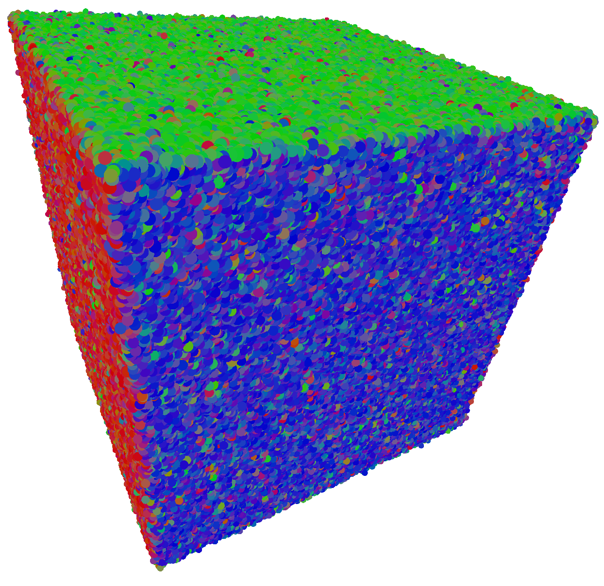
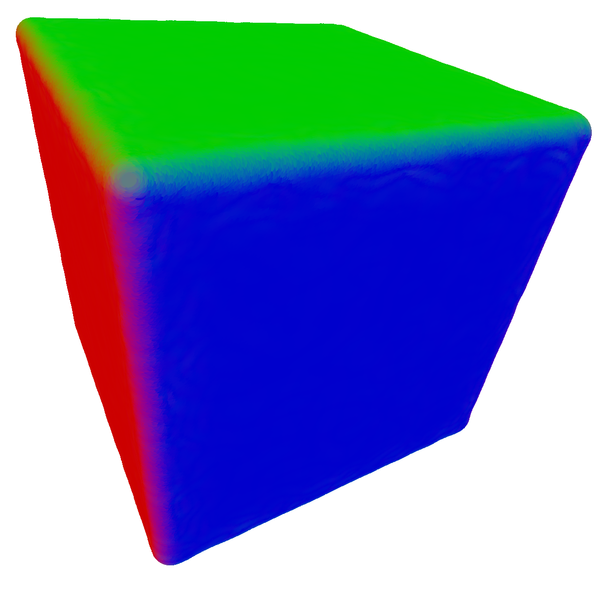
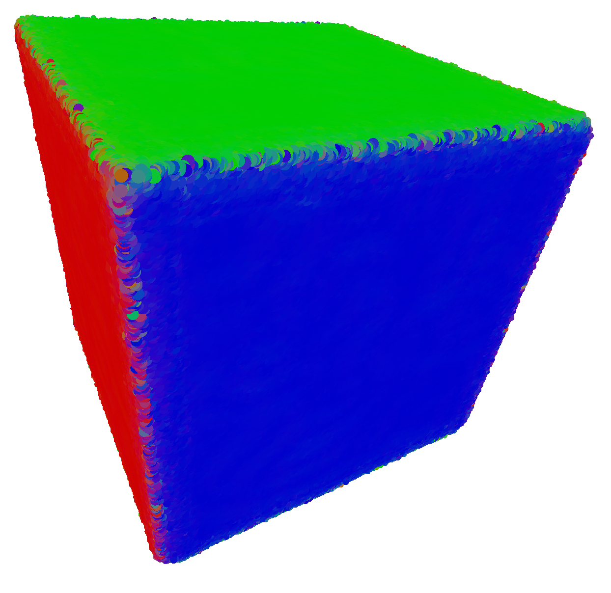
![[Uncaptioned image]](/html/1612.02261/assets/figures/cube_noisy_slice_crop_blue.png)
![[Uncaptioned image]](/html/1612.02261/assets/figures/cube_bilat_slice_crop_blue.png)
![[Uncaptioned image]](/html/1612.02261/assets/figures/cube_lpf_slice_crop_blue.png)
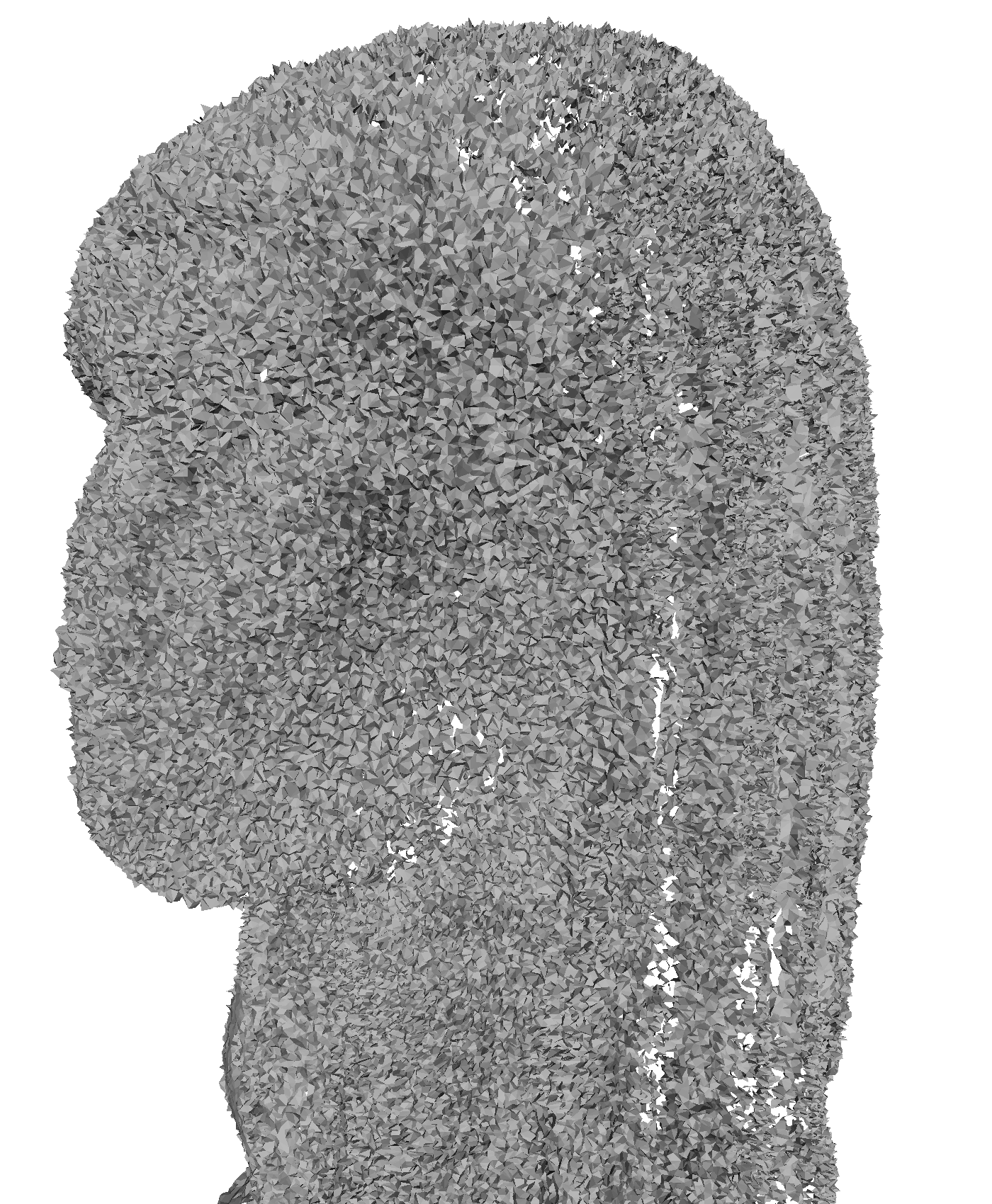
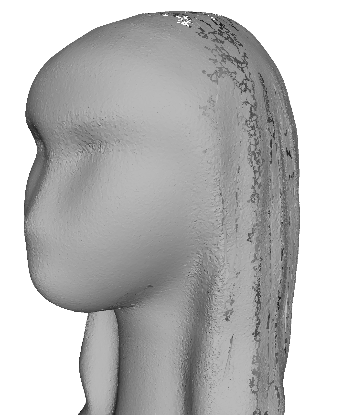
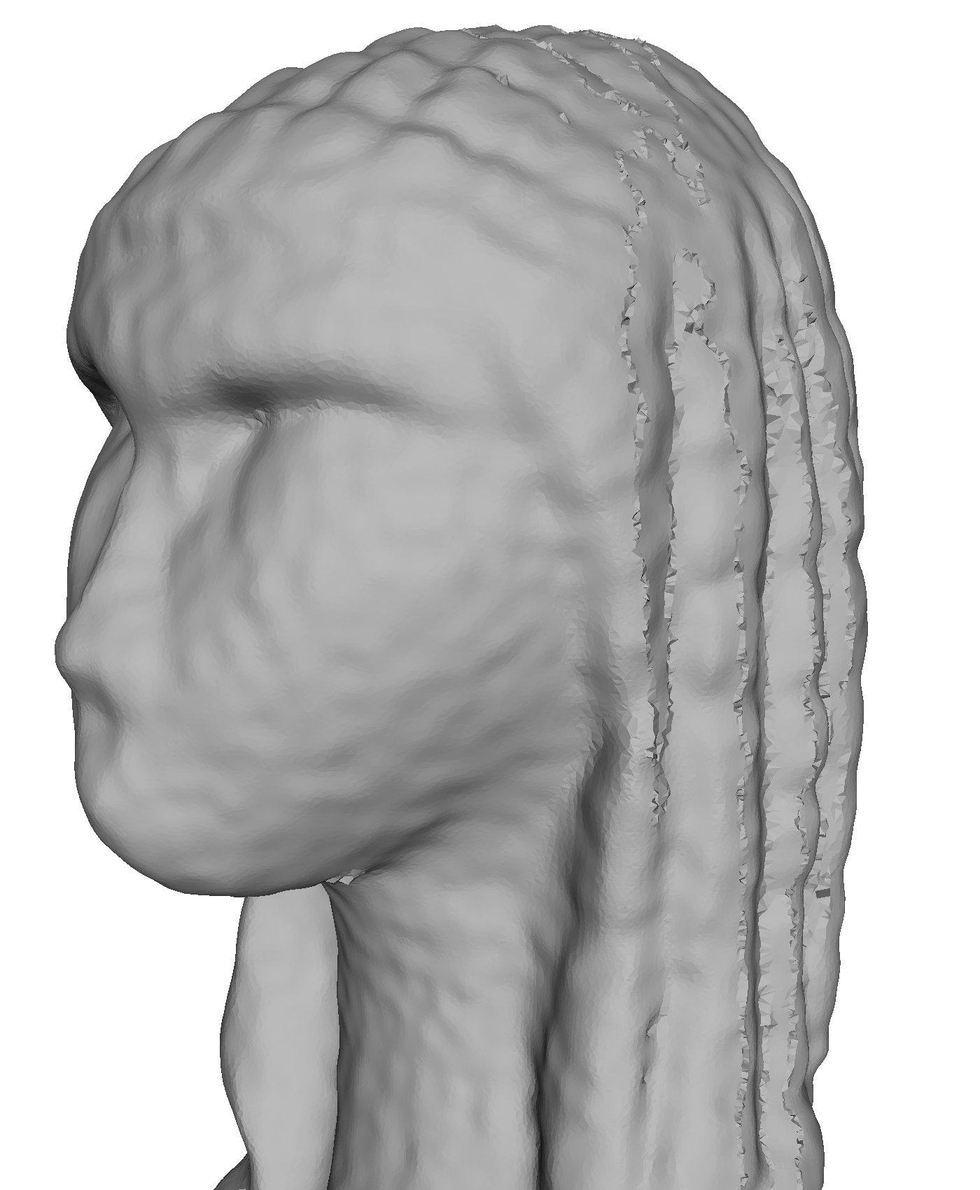
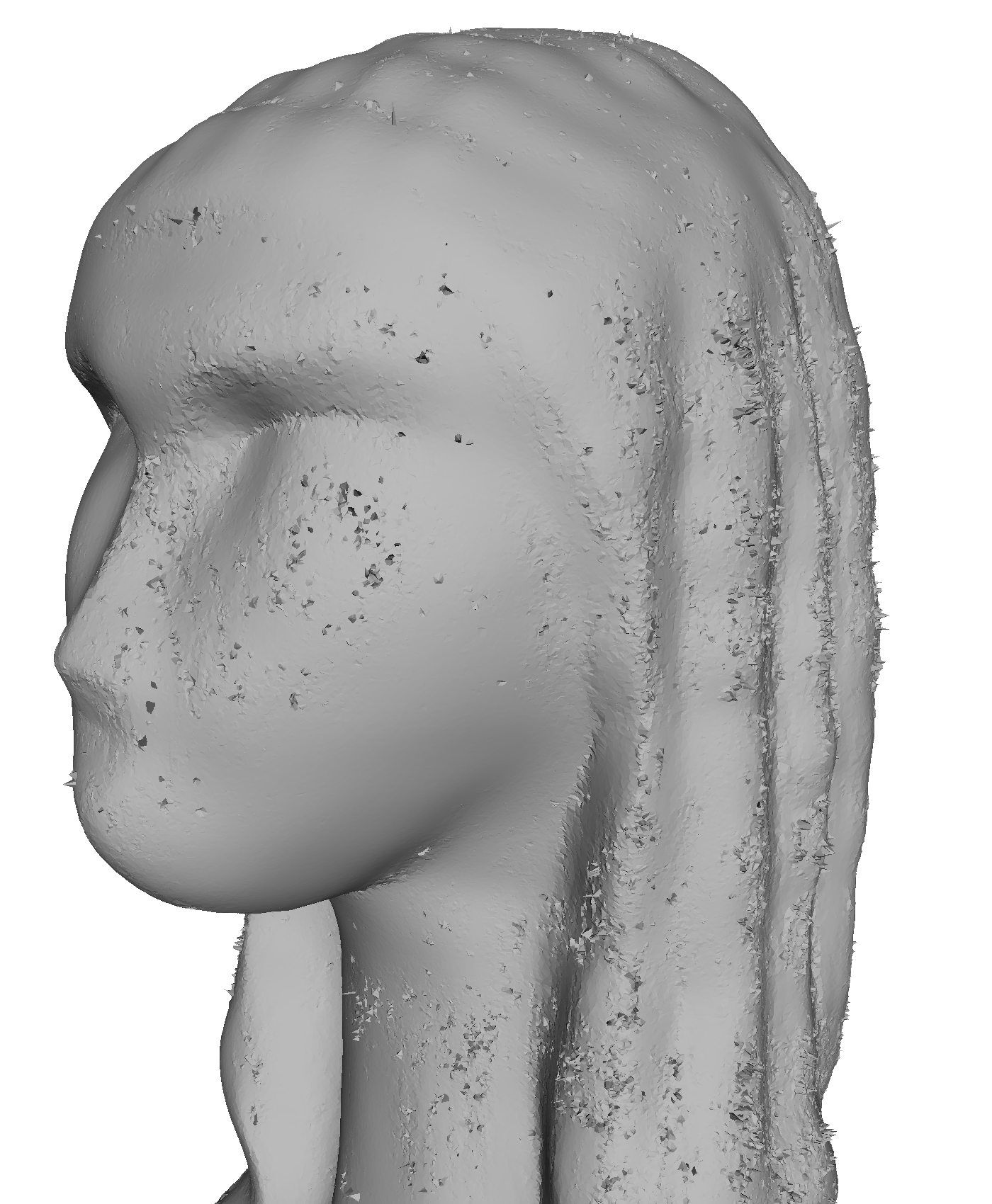
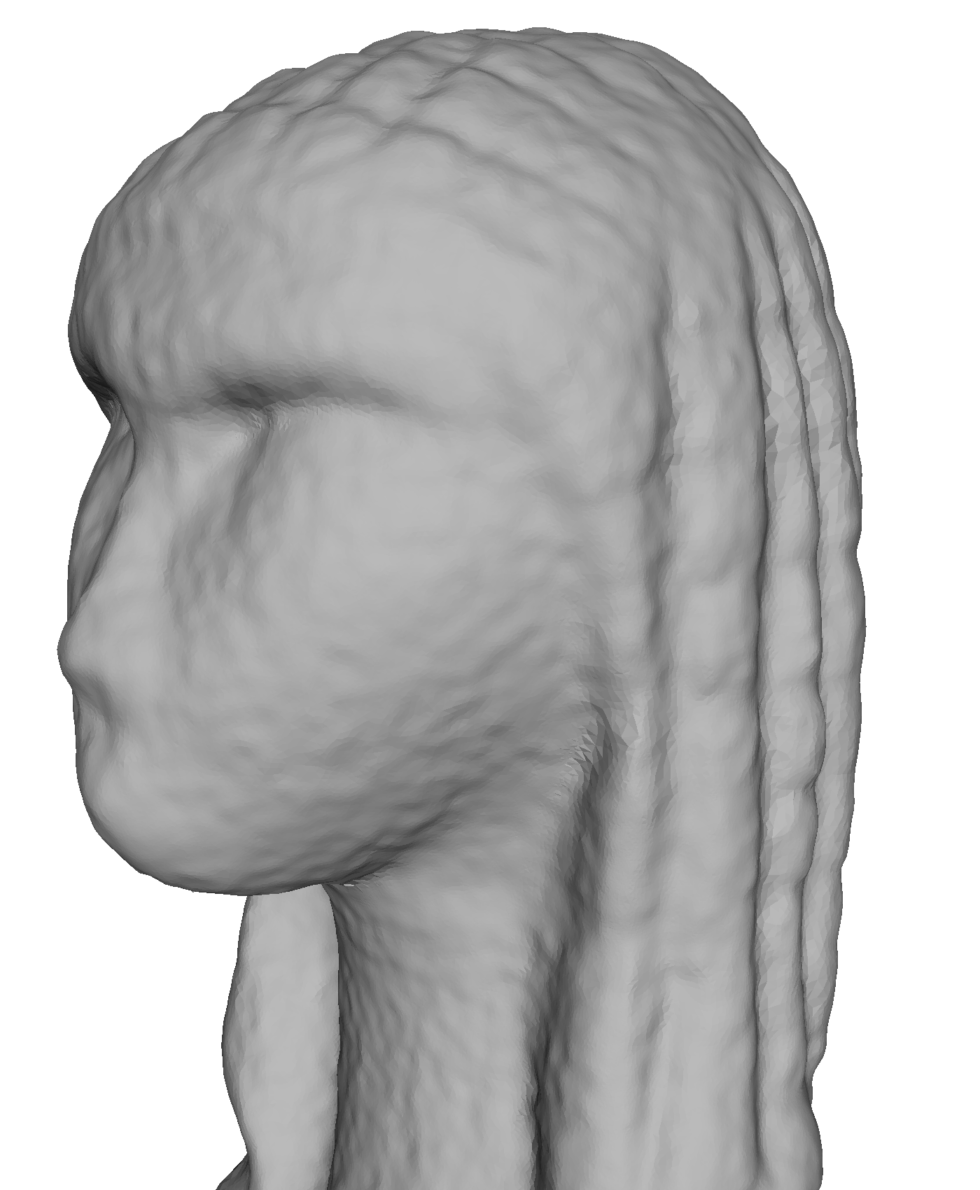

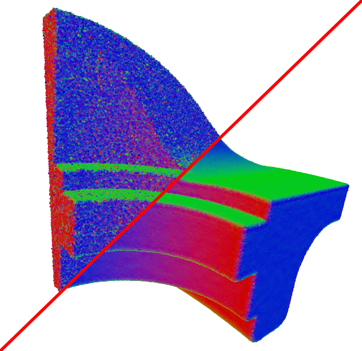
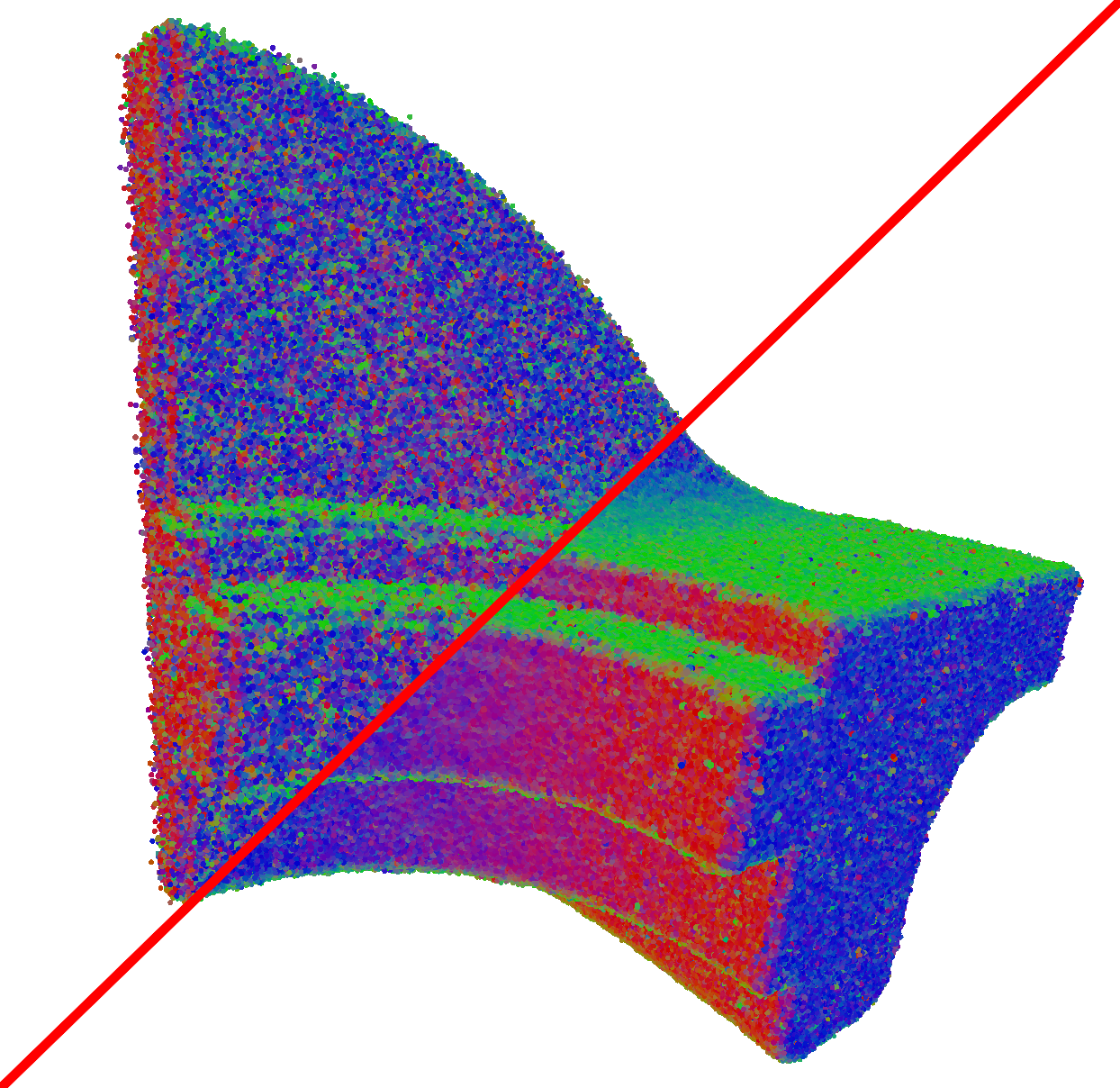
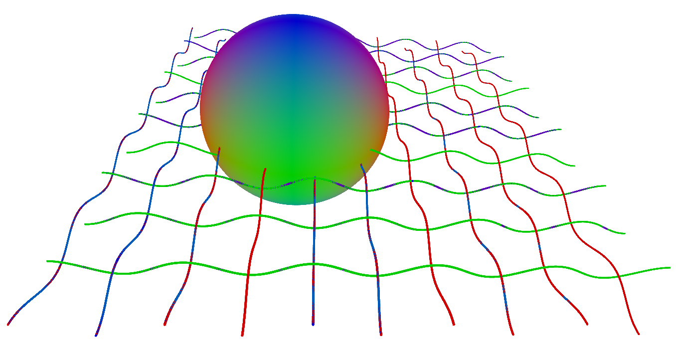
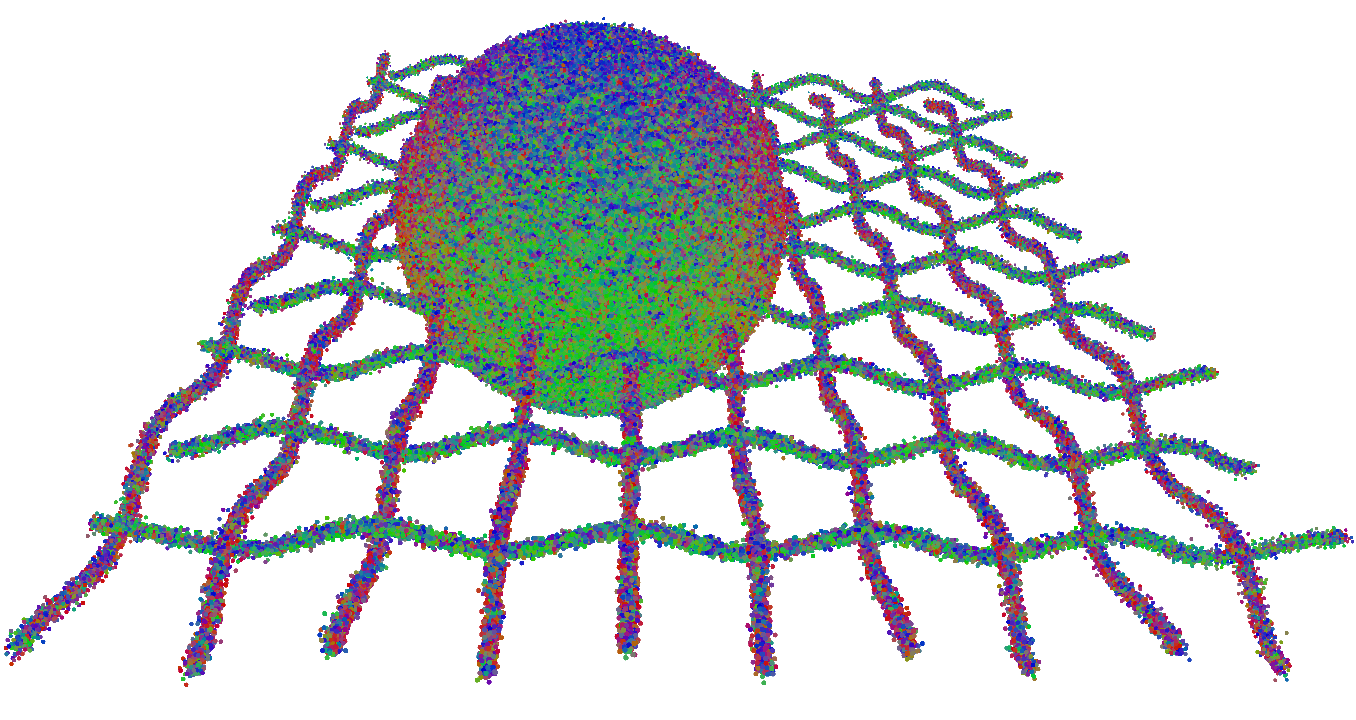
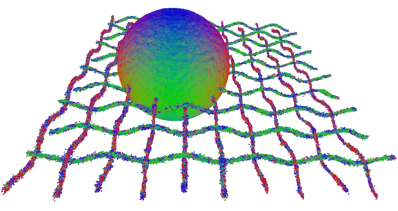
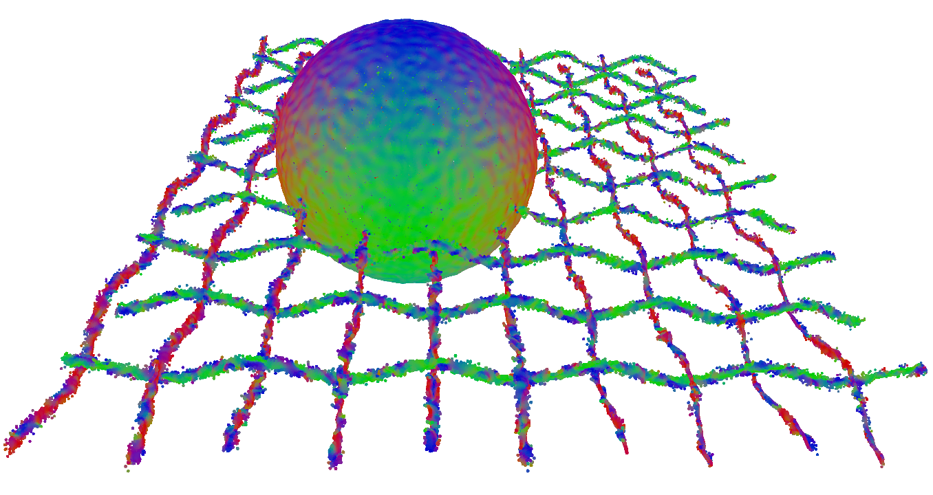
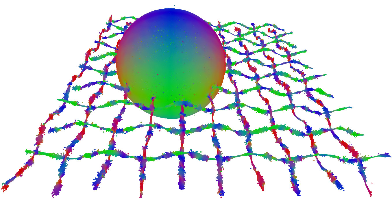
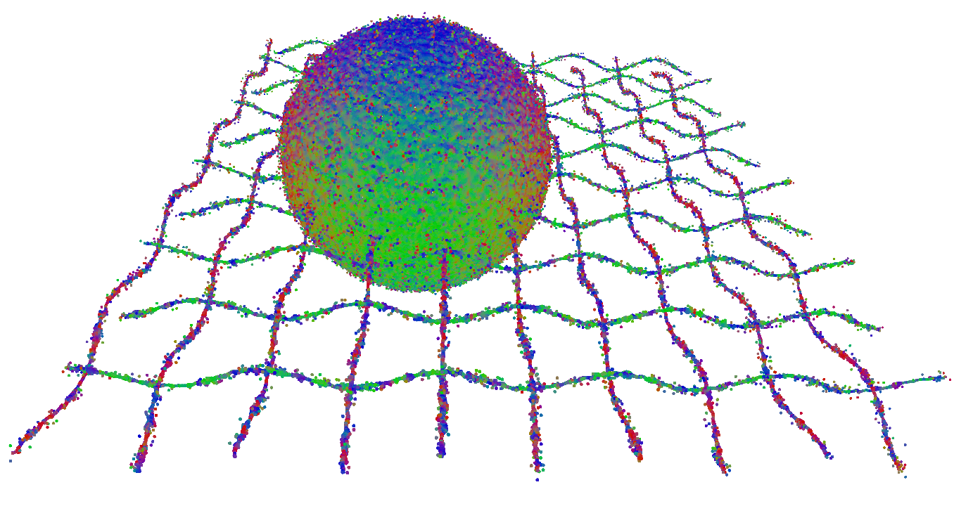
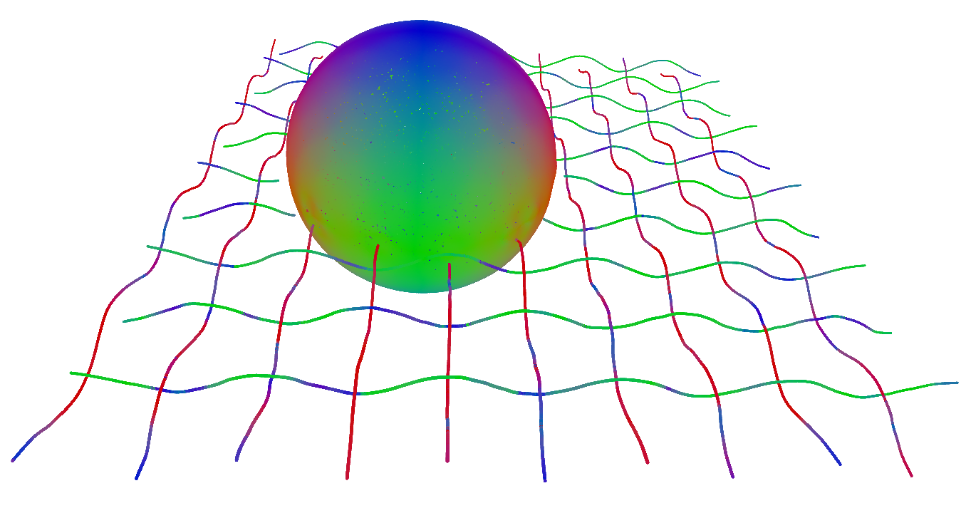
On Fig. 20 and Table I, we compare visually and quantitatively the performance of our denoising algorithm on a synthetic point cloud. Only our algorithm is able to denoise correctly both the surface and the curve net. Notice that Weighted Locally Optimal Projection (WLOP) [36] recovers the curves better than the other state-of-the art algorithms, although it is outperformed by our LPF approach.
4.3 Implementation details
Our algorithm was implemented in C++ using the Eigen library for matrix representation. For a non-optimized code and million input point set, covered by s with a pattern containing points (a pattern of points intersected with a sphere) and a dictionary of atoms, the initial computation took and the shape learning process took ( iterations of dictionary computation, pose estimation and recomputation) on a -core Intel®Core™i7 laptop.
5 Limitations
The principal limitation of our method is that it learns shapes in a statistical manner: an important feature that is not frequent enough will not be accounted for in the shape dictionary. As an example, no corner is present in the cube with curve dictionary (Figure 7). To overcome this limitation one could devise a strategy that adds more s where the representation error is largest. This would however require further analysis to ensure that the added information does not correspond to noise. Moreover, optimizing the shape of the template during analysis could also improve the results quality. One should notice that the dictionary is learned on a specific shape, and analyzing another shape might not be done as efficiently using the same dictionary, except if both shapes share local similarities.
Outliers are also a limitation of our method. Indeed, if a LPF is centered at an outlier position then the LPF will represent a single point. In the joint analysis this LPF will be replaced by a consolidated version which would have little sense. This can be easily alleviated by adding a preprocessing step to remove outliers.
Finally, our method requires some parameters: the user has to choose both the scale and the dictionary size. The choice of a scale can be argued for, since the analysis reveals different similarities depending on the chosen scale. The size of the dictionary is application and data-dependent; it should be large enough to encode shape variations but small enough for similarities to emerge. It is simple to set for geometric shapes, such as cubes, but more difficult for complex natural shapes. Selecting a good dictionary size is still an open issue that we want to explore in future works.
6 Conclusion and Future Work
We have introduced a pliable framework to analyze shapes by consolidating Local Probing Fields defined in the ambient space around the whole shape. By jointly analyzing this set of descriptions we provided a new tool for sparse shape description expressed as a dictionary learning problem. As demonstrated in our experiments, this tool allows the shape to reveal its non-local similarities. The efficiency of this framework is illustrated on shape resampling and point set denoising applications. As a future work we mean to study the theoretical properties of the Local Probing Fields and in particular possible improvements of the statistical properties of the consolidated point distribution. A whole set of applications of our framework remains to be explored, including shape compression, segmentation and registration, as well as the extension of our approach to shape collections.
Acknowledgments
This work was supported by the ANR PAPS project, grant ANR-14-CE27-0003 of the French Agence Nationale de la Recherche.
References
- [1] N. J. Mitra, M. Pauly, M. Wand, and D. Ceylan, “Symmetry in 3d geometry: Extraction and applications,” Computer Graphics Forum, vol. 32, no. 6, pp. 1–23, 2013.
- [2] M. Pauly, N. J. Mitra, J. Wallner, H. Pottmann, and L. J. Guibas, “Discovering structural regularity in 3d geometry,” ACM Transactions on Graphics, Proc SIGGRAPH’08, no. 3, pp. 43:1–43:11, 2008.
- [3] A. Buades, B. Coll, and J.-M. Morel, “A non-local algorithm for image denoising,” in IEEE Conference on Computer Vision and Pattern Recognition, 2005, pp. 60–65.
- [4] E. Shechtman and M. Irani, “Matching local self-similarities across images and videos,” 2007 IEEE Conference on Computer Vision and Pattern Recognition, pp. 1–8, 2007.
- [5] S. Yoshizawa, A. Belyaev, and H.-P. Seidel, “Smoothing by example: Mesh denoising by averaging with similarity-based weights,” in SMI ’06. IEEE, 2006, p. 9.
- [6] J. Digne, “Similarity based filtering of point clouds.” in CVPR Workshops. IEEE, 2012, pp. 73–79.
- [7] A. Hamdi-Cherif, J. Digne, and R. Chaine, “Super-resolution of point set surfaces using local similarities,” to appear in Computer Graphics Forum, 2017.
- [8] T. Guillemot, A. Almansa, and T. Boubekeur, “Non local point set surfaces,” in Proc. 3DIMPVT 2012, 2012, pp. 324–331.
- [9] A. Sharf, M. Alexa, and D. Cohen-Or, “Context-based surface completion,” ACM Transactions on Graphics, vol. 23, no. 3, pp. 878–887, 2004.
- [10] Q. Zheng, A. Sharf, G. Wan, Y. Li, N. J. Mitra, D. Cohen-Or, and B. Chen, “Non-local scan consolidation for 3d urban scenes,” ACM Transactions on Graphics, Proc. SIGGRAPH 10, 2010.
- [11] M. Aharon, M. Elad, and A. Bruckstein, “k -svd: An algorithm for designing overcomplete dictionaries for sparse representation,” IEEE Transactions on Signal Processing, vol. 54, 2006.
- [12] J. Mairal, F. Bach, J. Ponce, and G. Sapiro, “Online dictionary learning for sparse coding,” in International Conference on Machine Learning. ACM, 2009, pp. 689–696.
- [13] S. Xiong, J. Zhang, J. Zheng, J. Cai, and L. Liu, “Robust surface reconstruction via dictionary learning,” ACM Transactions On Graphics, Proc. SIGGRAPH Asia 2014, vol. 33, 2014.
- [14] R. Litman, A. Bronstein, M. Bronstein, and U. Castellani, “Supervised learning of bag-of-features shape descriptors using sparse coding,” Computer Graphics Forum, vol. 33, no. 5, pp. 127–136, 2014.
- [15] J. Digne, R. Chaine, and S. Valette, “Self-similarity for accurate compression of point sampled surfaces,” Computer Graphics Forum, vol. 33, no. 2, pp. 155–164, 2014, proceedings of Eurographics 2014.
- [16] L. Xu, R. Wang, J. Zhang, Z. Yang, J. Deng, F. Chen, and L. Liu, “Survey on sparsity in geometric modeling and processing,” Graphical Models, vol. 82, pp. 160 – 180, 2015.
- [17] Y. Lipman, O. Sorkine, D. Cohen-Or, D. Levin, C. Rossi, and H.-P. Seidel, “Differential coordinates for interactive mesh editing,” in Proc. SMI 2004. IEEE, 2004, pp. 181–190.
- [18] O. Sorkine, D. Cohen-Or, Y. Lipman, M. Alexa, C. Rössl, and H.-P. Seidel, “Laplacian surface editing,” Computer Graphics Forum (Proc. SGP 2004), pp. 179–188, 2004.
- [19] R. Wang, L. Liu, Z. Yang, K. Wang, W. Shan, J. Deng, and F. Chen, “Construction of manifolds via compatible sparse representations,” ACM Transactions on Graphics, vol. 35, no. 2, pp. 14:1–14:10, 2016.
- [20] D. G. Lowe, “Distinctive image features from scale-invariant keypoints,” International journal of computer vision, vol. 60, no. 2, pp. 91–110, 2004.
- [21] A. E. Johnson and M. Hebert, “Using spin images for efficient object recognition in cluttered 3d scenes,” IEEE Transactions on Pattern Analysis and Machine Intelligence, vol. 21, pp. 433–449, 1999.
- [22] F. Tombari, S. Salti, and L. Di Stefano, “Unique signatures of histograms for local surface description,” in IEEE European Conference on Computer Vision. Springer-Verlag, 2010, pp. 356–369.
- [23] S. Belongie, J. Malik, and J. Puzicha, “Shape matching and object recognition using shape contexts,” IEEE Transactions on Pattern Analysis and Machine Intelligence, vol. 24, pp. 509–522, 2002.
- [24] I. Kokkinos, M. M. Bronstein, R. Litman, and A. M. Bronstein, “Intrinsic shape context descriptors for deformable shapes,” in IEEE Conference on Computer Vision and Pattern Recognition, June 2012, pp. 159–166.
- [25] A. Zaharescu, E. Boyer, K. Varanasi, and R. Horaud, “Surface feature detection and description with applications to mesh matching,” in IEEE Conference on Computer Vision and Pattern Recognition, June 2009, pp. 373–380.
- [26] J. Sun, M. Ovsjanikov, and L. Guibas, “A concise and provably informative multi-scale signature based on heat diffusion,” Computer Graphics Forum (Proc. SGP 2009), pp. 1383–1392, 2009.
- [27] N. Li, S. Wang, M. Zhong, Z. Su, and H. Qin, “Generalized local-to-global shape feature detection based on graph wavelets,” IEEE Transactions on Visualization and Computer Graphics, vol. 22, no. 9, pp. 2094–2106, Sept 2016.
- [28] A. M. Bronstein, M. M. Bronstein, L. J. Guibas, and M. Ovsjanikov, “Shape google: Geometric words and expressions for invariant shape retrieval,” ACM Transactions on Graphics, vol. 30, pp. 1–20, 2011.
- [29] O. Mattausch, D. Panozzo, C. Mura, O. Sorkine-Hornung, and R. Pajarola, “Object detection and classification from large-scale cluttered indoor scans,” Computer Graphics Forum, vol. 33, no. 2, pp. 11–21, 2014.
- [30] L. Wei, Q. Huang, D. Ceylan, E. Vouga, and H. Li, “Dense human body correspondences using convolutional networks,” CoRR, vol. abs/1511.05904, 2015.
- [31] J. Masci, D. Boscaini, M. M. Bronstein, and P. Vandergheynst, “Geodesic convolutional neural networks on riemannian manifolds,” in ICCV Workshops 2015. IEEE, 2015.
- [32] D. Boscaini, J. Masci, E. Rodolà, and M. M. Bronstein, “Learning shape correspondence with anisotropic convolutional neural networks,” CoRR, vol. abs/1605.06437, 2016.
- [33] H. Huang, D. Li, H. Zhang, U. Ascher, and D. Cohen-Or, “Consolidation of unorganized point clouds for surface reconstruction,” ACM Transactions on Graphics, vol. 28, pp. 176:1–176:78, 2009.
- [34] H. Huang, S. Wu, M. Gong, D. Cohen-Or, U. Ascher, and H. R. Zhang, “Edge-aware point set resampling,” ACM Transactions on Graphics, vol. 32, no. 1, pp. 9:1–9:12, Feb. 2013.
- [35] Y. Lipman, D. Cohen-Or, D. Levin, and H. Tal-Ezer, “Parameterization-free projection for geometry reconstruction,” ACM Transactions on Graphics, vol. 26, 2007.
- [36] H. Huang, D. Li, H. Zhang, U. Ascher, and D. Cohen-Or, “Consolidation of unorganized point clouds for surface reconstruction,” in SIGGRAPH Asia 2009. ACM, 2009, pp. 176:1–176:7.
- [37] M. Alexa, J. Behr, D. Cohen-Or, S. Fleishman, D. Levin, and C. T. Silva, “Point set surfaces,” in Proc. Vis ’01. IEEE, 2001, pp. 21–28.
- [38] N. Amenta and Y. J. Kil, “Defining point-set surfaces,” in SIGGRAPH ’04. USA: ACM Press, 2004, pp. 264–270.
- [39] S. Fleishman, D. Cohen-Or, and C. T. Silva, “Robust moving least-squares fitting with sharp features,” ACM Transactions on Graphics, vol. 24, no. 3, pp. 544–552, 2005.
- [40] G. Guennebaud and M. Gross, “Algebraic point set surfaces,” ACM Transactions on Graphics, vol. 26, 2007, proc. SIGGRAPH 2007.
- [41] A. C. Oztireli, G. Guennebaud, and M. Gross, “Feature preserving point set surfaces based on non-linear kernel regression,” Computer Graphics Forum, vol. 28, pp. 493–501(9), 2009.
- [42] S. Wu, H. Huang, M. Gong, M. Zwicker, and D. Cohen-Or, “Deep points consolidation,” ACM Transactions on Graphics, vol. 34, no. 6, pp. 176:1–176:13, 2015.
- [43] R. Wang, Z. Yang, L. Liu, J. Deng, and F. Chen, “Decoupling noise and features via weighted -analysis compressed sensing,” ACM Transactions on Graphics, vol. 33, no. 2, pp. 18:1–18:12, Apr. 2014.
- [44] Y. Sun, S. Schaefer, and W. Wang, “Denoising point sets via minimization,” Computer Aided Geometric Design, vol. 35–36, pp. 2 – 15, 2015, geometric Modeling and Processing 2015.
- [45] H. Zhang, C. Wu, J. Zhang, and J. Deng, “Variational mesh denoising using total variation and piecewise constant function space,” IEEE Transactions on Visualization and Computer Graphics, vol. 21, no. 7, pp. 873–886, July 2015.
- [46] X. Lu, Z. Deng, and W. Chen, “A robust scheme for feature-preserving mesh denoising,” IEEE Transactions on Visualization and Computer Graphics, vol. 22, no. 3, pp. 1181–1194, March 2016.
- [47] M. Wei, J. Yu, W. M. Pang, J. Wang, J. Qin, L. Liu, and P. A. Heng, “Bi-normal filtering for mesh denoising,” IEEE Transactions on Visualization and Computer Graphics, vol. 21, no. 1, pp. 43–55, Jan 2015.
- [48] P. J. Besl and N. D. McKay, “A method for registration of 3-d shapes,” IEEE Transactions Pattern Analysis and Machine Intelligence, vol. 14, no. 2, pp. 239–256, 1992.
- [49] J. Mairal, F. Bach, J. Ponce, and G. Sapiro, “Online learning for matrix factorization and sparse coding,” J. Mach. Learn. Res., vol. 11, pp. 19–60, 2010.
- [50] B. Efron, T. Hastie, I. Johnstone, and R. Tibshirani, “Least angle regression,” Annals of Statistics, vol. 32, pp. 407–499, 2004.
- [51] M. Kazhdan and H. Hoppe, “Screened poisson-surface reconstruction,” ACM Transactions on Graphics, 2013.
- [52] H. Hoppe, T. DeRose, T. Duchamp, J. McDonald, and W. Stuetzle, “Surface reconstruction from unorganized points,” in SIGGRAPH ’92, 1992, pp. 71–78.
- [53] M. Elad and M. Aharon, “Image denoising via sparse and redundant representations over learned dictionaries,” IEEE Transactions on Image Processing, vol. 15, no. 12, pp. 3736–3745, Dec 2006.
- [54] S. Fleishman, I. Drori, and D. Cohen-Or, “Bilateral mesh denoising,” ACM Transactions on Graphics, vol. 22, no. 3, pp. 950–953, 2003.
![[Uncaptioned image]](/html/1612.02261/assets/figures/digne.png) |
Julie Digne Julie Digne is a junior CNRS researcher at LIRIS laboratory working in Geometry Processing. She obtained her PhD in 2010 in applied mathematics at Ecole Normale Supérieure de Cachan in 2010, which was awarded the Jacques Hadamard Foundation for Mathematics PhD award. She was a post-doc at INRIA. She joined the GeoMod team at LIRIS, University of Lyon in 2012, her current work focuses on point set surface processing including denoising and super-resolution. |
![[Uncaptioned image]](/html/1612.02261/assets/figures/valette.png) |
Sébastien Valette Sébastien Valette is a CNRS Researcher at CREATIS, Lyon, France. He recieved the Electrical Engineering degree and PhD Degree at INSA-Lyon in 2002. His research interests include geometry processing, data compression and image analysis. |
![[Uncaptioned image]](/html/1612.02261/assets/figures/RaphaelleChaine.jpeg) |
Raphaëlle Chaine ’s research interests include geometry processing, geometric modeling and virtual sculpture. She graduated with the M.S. Degree at Ecole Centrale de Lyon in 1995. After completing her PhD in computer science from the Université Claude Bernard in France, in the domain of point set surfaces analysis, she joined the PRISME Geometrica team at INRIA Sophia Antipolis in 2000. There, she focused her work on 3D reconstruction and computational geometry. In 2003 Raphaëlle joined the LIRIS (CNRS) laboratory where she was promoted to a professor position in 2013 at Lyon 1 University. |