Renormalization of fermion velocity in finite temperature QED₃

Abstract

At zero temperature, the Lorentz invariance is strictly preserved in three-dimensional quantum electrodynamics. This property ensures that the velocity of massless fermions is not renormalized by the gauge interaction. At finite temperature, however, the Lorentz invariance is explicitly broken by the thermal fluctuation. The longitudinal component of gauge interaction becomes short-ranged due to thermal screening, whereas the transverse component remains long-ranged because of local gauge invariance. The transverse gauge interaction leads to singular corrections to the fermion self-energy and thus results in an unusual renormalization of the fermion velocity. We calculate the renormalized fermion velocity $v^{R}(p_{0},\mathbf{p},T)$ by employing a renormalization group analysis, and discuss the influence of the anomalous dimension $\eta_{n}$ on the fermion specific heat.

Four-dimensional quantum electrodynamics (QED₄) can describe the electromagnetic interaction with very high precision after eliminating ultraviolet divergences by means of renormalization method. Different from QED₄, (2+1)-dimensional QED of massless fermions, dubbed QED₃, is superrenormalizable and does not contain any ultraviolet divergence. However, extensive investigations have showed that QED₃ exhibits a series of nontrivial low-energy properties, such as dynamical chiral symmetry breaking (DCSB) Pisarski84 ; Appelquist86 ; Appelquist88 ; Nash89 ; Atkinson90 ; Curtis90 ; Pennington91 ; Curtis92 ; Maris96 ; Fisher04 ; Bashir08 ; Bashir09 ; Goecke09 ; Lo11 ; Braun14 ; Roberts94 ; Appelquist04 , asymptotic freedom Appelquist86 , and weak confinement Burden92 ; Maris95 ; Bashir08 . It thus turns out that QED₃ is more similar to four-dimensional quantum chromodynamics (QCD₄) than QED₄. For this reason, QED₃ is widely regarded as a toy model of QCD₄ in high-energy physics. On the other hand, in the past decades QED₃ has proven to be an effective low-energy field theory for several important condensed-matter systems, including high-$T_{c}$ cuprate superconductors Lee06 ; Affleck ; Kim97 ; Kim99 ; Rantner ; Franz ; Herbut ; Liu02 ; Liu03 , spin-$1/2$ Kagome spin liquid Ran07 ; Hermele08 , graphene Gusynin04 ; Gusynin07 ; Raya08 , certain quantum critical systems Klebanov ; Lu14 , surface states of some bulk topological insulators Metlitski15 ; Wang15 ; Mross15 .

Appelquist et al. analyzed the Dyson-Schwinger equation (DSE) of fermion mass in zero-$T$ QED₃ and revealed that the massless fermions can acquire a finite dynamical mass, which induces DCSB, when the fermion flavor is below some threshold, i.e., $N<N_{c}$ Appelquist88 . Most existing analytical and numerical calculations Nash89 ; Atkinson90 ; Curtis90 ; Pennington91 ; Curtis92 ; Maris96 ; Fisher04 ; Roberts94 ; Appelquist04 agree that $N_{c}\approx 3.5$ at zero $T$. This problem is not only interesting in its own right, but of practical importance since QED₃ has wide applications in condensed-matter physics Lee06 ; Affleck ; Kim97 ; Kim99 ; Rantner ; Franz ; Herbut ; Liu02 ; Liu03 ; Ran07 ; Hermele08 ; Gusynin04 ; Gusynin07 ; Raya08 ; Klebanov ; Lu14 ; Metlitski15 ; Wang15 ; Mross15 . In particular, it has been demonstrated Affleck ; Kim97 ; Kim99 ; Liu02 ; Franz ; Herbut that DCSB leads to the formation of quantum antiferromagnetism. Dynamical mass generation at finite temperature in QED₃ is also an interesting, and meanwhile very complicated, issue that has been investigated for over two decades Dorey92 ; Lee98 ; Triantaphyllou ; Feng13 ; Feng14 ; Lo14 ; WangLiuZhang15 .

If the fermion flavor is large, say $N\geq 4$, no DCSB takes place and the Dirac fermions are still massless despite of the presence of strong gauge interaction. However, QED₃ is still highly nontrivial in its massless phase, because the gauge interaction can lead to unusual, non-Fermi liquid like behaviors of fermions Kim97 ; Kim99 ; WangLiu10A ; WangLiu10B . These non-Fermi liquid behaviors may be of important relevance to the low-energy physics of high-$T_{c}$ cuprate superconductors Kim97 ; Kim99 ; Lee06 and other strongly correlated systems.

When studying the non-Fermi liquid behaviors of massless fermions, an important role is known to be played by the fermion velocity $v$, which enters into many observable quantities of massless fermions, such as specific heat Kim97 ; Vafek07 ; Xu08 ; JWangLiu12 ; Liu2015 and thermal conductivity Fritz09 . An interesting property is that the constant velocity can be renormalized by various interactions and then exhibits unusual momentum dependence. For instance, it is known that the low-energy elementary excitations of graphene, a single layer of carbon atoms, are massless Dirac fermions Kotov . The fermion velocity in graphene is certainly a constant in the non-interacting limit, and its bare value is roughly $c/300$ with $c$ being the speed of light in vacuum Kotov . However, extensive renormalization group (RG) analysis Gonzalez94 ; Gonzalez99 ; Son07 ; Kotov have showed that the fermion velocity can be enhanced by the unscreened long-range Coulomb interaction. In the lowest energy limit, the velocity flows to very large values and the fermion dispersion is thus substantially modified. Remarkably, the predicted nearly divergence of the renormalized velocity has already been confirmed in recent experiments Elias11 ; Yu13 ; Siegel12 . Another notable example is the effective QED₃ theory of high-$T_{c}$ superconductors Lee06 ; Kim97 ; Kim99 , which contains only the transverse part of the U(1) gauge interaction. Moreover, near the nematic quantum critical point in high-$T_{c}$ superconductors, massless Dirac fermions interact strongly with the quantum fluctuation of nematic order parameter Huh08 ; Wang11 ; Liu12 ; She15 . In both cases, the fermion velocity receives singular corrections and is driven to vanish in the low-energy region Lee06 ; Kim97 ; Kim99 ; Huh08 ; Wang11 ; Liu12 ; She15 , which in turn results in non-Fermi liquid behaviors Lee06 ; Kim97 ; Kim99 ; Liu2015 .

In this paper, we study the renormalization of fermion velocity due to U(1) gauge interaction in QED₃. Whether the velocity is renormalized depends crucially on the temperature of the system. At zero temperature, the Lorentz invariance of QED₃ is certainly reserved, and thus there is no interaction corrections to the fermion velocity. In this case, fermion velocity is always a constant. At finite temperature, however, the Lorentz invariance is explicitly broken by thermal fluctuations Dorey92 . As a result, the longitudinal and transverse parts of the gauge interaction are no longer identical, and the fermion velocity may flow with varying energy and momenta. It is interesting to ask two questions: How the fermion velocity is renormalized by the gauge interaction at finite temperature? How the physical quantities of Dirac fermions, such as the specific heat, are influenced by the renormalzied velocity? In this article, we will study these two questions.

We study this problem and calculate the renormalized fermion velocity $v^{R}(p_{0},\mathbf{p},T)$ by means of renormalization group method. We show that the velocity exhibits a power law dependence on momentum $|\mathbf{p}|$ under the energy scale $T$,

$$v^{R}(p_{0},\mathbf{p},T)=\left(\frac{|\mathbf{p}|}{T}\right)^{\eta},$$ (1)

where the anomalous dimension $\eta$ are functions of both $T$ and energy $p_{0}$, namely $\eta\equiv\eta(p_{0},T)$. We then study the impact of the renormalized fermion velocity on the specific heat of massless Dirac fermions.

The Lagrangian density for QED₃ with $N$ flavors of massless Dirac fermions is given by

$$\mathcal{L}=\sum_{i=1}^{N}\bar{\psi}_{i}\left(i\partial\!\!\!/+eA\!\!\!/\right)\psi_{i}-\frac{1}{4}F_{\mu\nu}^{2},$$ (2)

where $F_{\mu\nu}=\partial_{\mu}A_{\nu}-\partial_{\nu}A_{\mu}$. The fermion is described by a four-component spinor $\psi$, whose conjugate is $\bar{\psi}=\psi^{{\dagger}}\gamma_{0}$. The gamma matrices are defined as $(\gamma_{0},\gamma_{1},\gamma_{2})=(i\sigma_{3},i\sigma_{1},i\sigma_{2})\otimes\sigma_{3}$, which satisfy the Clifford algebra $\{\gamma_{\mu},\gamma_{\nu}\}=2g_{\mu\nu}$ with $g_{\mu\nu}=\mathrm{diag}(-1,-1,-1)$. In (2+1) dimensions, there are two chiral matrices, denoted by $\gamma_{3}=I_{2\times 2}\otimes\sigma_{1}$ and $\gamma_{5}=I_{2\times 2}\otimes\sigma_{2}$ respectively, that anti-commute with $\gamma_{0,1,2}$. This Lagrangian respects a continuous $U(2N)$ chiral symmetry $\psi\rightarrow e^{i\theta\gamma_{3,5}}\psi$, where $\theta$ is an arbitrary constant. Once fermions become massive, the $U(2N)$ chiral symmetry is broken down to $U(N)\times U(N)$. Here, we consider a general very large $N$, which implies the absence of DCSB, and perform perturbative expansion in powers of $1/N$. For simplicity, we work in units with $\hbar=k_{B}=1$.

The fermions have a constant velocity $v$, which appears in the covariant derivative in the form $\partial\!\!\!/=\gamma_{0}\partial_{0}+v\mathbf{\gamma}\cdot\mathbf{\nabla}$. In most previous studies, it is assumed that $v\equiv 1$. At zero $T$, this assumption is perfectly good and not affected by the gauge interaction since the Lorentz invariance is absolutely satisfied. To see this, we write the fermion propagator as

$$G_{0}(k_{0},\mathbf{k})=\frac{1}{\gamma_{0}k_{0}+v\mathbf{\gamma}\cdot\mathbf{k}}.$$ (3)

The self-energy corrections due to gauge interaction is generically expressed as

$$\Sigma(k_{0},\mathbf{k})=A_{0}(k_{0},\mathbf{k})\gamma_{0}k_{0}+A_{\mathrm{s}}(k_{0},\mathbf{k})v\mathbf{\gamma}\cdot\mathbf{k}.$$ (4)

Here, $A_{0,\mathrm{s}}(k_{0},\mathbf{k})$ are the temporal and spatial components of the wave function renormalization respectively. At $T=0$, the Lorentz invariance ensures that

$$A_{0}(k_{0},\mathbf{k})=A_{\mathrm{s}}(k_{0},\mathbf{k})\equiv A(k),$$ (5)

thus the dressed fermion propagator has the form

$$G(k_{0},\mathbf{k})=\frac{1}{\left[1+A(k)\right]\left(\gamma_{0}k_{0}+v\mathbf{\gamma}\cdot\mathbf{k}\right)}.$$ (6)

Clearly, the velocity $v$ remains a constant and does not receive any interaction corrections. It is therefore safe to set $v\equiv 1$. However, this is no longer true when the Lorentz invariance is explicitly broken at finite $T$. Once the Lorentz invariance is broken, we have $A_{0}(k_{0},\mathbf{k})\neq A_{\mathrm{s}}(k_{0},\mathbf{k})$. The difference $\Delta A=A_{\mathrm{s}}(k_{0},\mathbf{k})-A_{0}(k_{0},\mathbf{k})$ represents the interaction correction to the fermion velocity $v$, which then becomes a function of energy-momenta and temperature, i.e., $v\rightarrow v^{R}(p_{0},\mathbf{p},T)$. We now calculate the function $v^{R}(p_{0},\mathbf{p},T)$ by means of RG method.

We will work in the standard Mastubara formalism for finite $T$ quantum field theory, and assume the fermion energy to be of the form $k_{0}=(2n+1)\pi T$ with $n$ being an integer. Including the correction of the polarizations, the effective propagator of gauge boson now becomes

$$\Delta_{\mu\nu}(q_{0},\mathbf{q}) = \frac{A_{\mu\nu}}{\frac{q_{0}^{2}}{v^{2}}+\mathbf{q}^{2}+\Pi_{A}(q_{0},\mathbf{q})}$$ (7)

$$+ \frac{B_{\mu\nu}}{\frac{q_{0}^{2}}{v^{2}}+\mathbf{q}^{2}+\Pi_{B}(q_{0},\mathbf{q})},$$

where $q_{0}=2m\pi T$ with $m$ being an integer. The two tensors $A_{\mu\nu}$ and $B_{\mu\nu}$ are defined as

$$A_{\mu\nu} = \left(\delta_{\mu 0}-\frac{q_{\mu}q_{0}}{q^{2}}\right)\frac{q^{2}}{v^{2}\mathbf{q}^{2}}\left(\delta_{0\nu}-\frac{q_{0}q_{\nu}}{q^{2}}\right),$$ (8)

$$B_{\mu\nu} = \delta_{\mu i}\left(\delta_{ij}-\frac{q_{i}q_{j}}{\mathbf{q}^{2}}\right)\delta_{j\nu}.$$ (9)

It is easy to verify that $A_{\mu\nu}$ and $B_{\mu\nu}$ are orthogonal and satisfy

$$A_{\mu\nu}+B_{\mu\nu}=\delta_{\mu\nu}-\frac{q_{\mu}q_{\nu}}{q^{2}}.$$ (10)

The polarizations $\Pi_{A}$ and $\Pi_{B}$ are defined by

$$\Pi_{A}=\frac{q^{2}}{v^{2}\mathbf{q}^{2}}\Pi_{00},\qquad\Pi_{B}=\Pi_{ii}-\frac{q_{0}^{2}}{v^{2}\mathbf{q}^{2}}\Pi_{00}$$ (11)

where

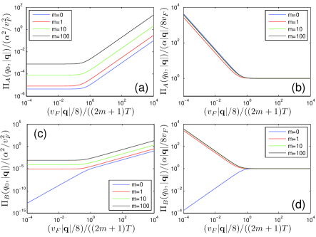
Figure 1: Polarizations $\Pi_{A}(q_{0},|\mathbf{q}|)$ and $\Pi_{B}(q_{0},|\mathbf{q}|)$ for different frequencies. Here, $q_{0}=2m\pi T$ and $T$ is chosen as $T/\alpha=10^{-5}$.

$$\Pi_{00} = \frac{\alpha}{\beta}\sum_{k_{0}}\int\frac{d^{2}\mathbf{k}}{(2\pi)^{2}}\mathrm{Tr}\left[G(k_{0},\mathbf{k})\gamma_{0}G(k_{0}+q_{0},\mathbf{k}+\mathbf{q})\gamma_{0}\right],$$

$$\Pi_{ii} = \frac{\alpha}{\beta}\sum_{k_{0}}\int\frac{d^{2}\mathbf{k}}{(2\pi)^{2}}\mathrm{Tr}\left[G(k_{0},\mathbf{k})\gamma_{i}G(k_{0}+q_{0},\mathbf{k}+\mathbf{q})\gamma_{i}\right],$$

with $\alpha=Ne^{2}$. As usual Appelquist88 , the parameter $\alpha$ is kept fixed as $N\rightarrow+\infty$. Employing the method utilized in Ref. Dorey92 , one can obtain the following expressions:

$$\Pi_{A}=\Pi_{3},\qquad\Pi_{B}=\Pi_{1}+\Pi_{2}$$ (12)

where

$$\Pi_{1} = \frac{\alpha}{2\pi v^{2}}\int_{0}^{1}dx\frac{\chi\sinh\left(\frac{\chi}{T}\right)}{\cosh^{2}\left(\frac{\chi}{2T}\right)-\sin^{2}\left(\frac{x\ q_{0}}{2T}\right)},$$

$$\Pi_{2} = \frac{\alpha q_{0}}{4\pi v^{2}}\int_{0}^{1}dx\frac{(1-2x)\sin\left(\frac{xq_{0}}{T}\right)}{\cosh^{2}\left(\frac{\chi}{2T}\right)-\sin^{2}\left(\frac{xq_{0}}{2T}\right)},$$

$$\Pi_{3} = \frac{\alpha T}{\pi v^{2}}\int_{0}^{1}dx$$

$$\times\ln\left(4\left[\cosh^{2}\left(\frac{\chi}{2T}\right)-\sin^{2}\left(\frac{xq_{0}}{2T}\right)\right]\right),$$

Figure 2: Polarizations $\Pi(q_{0},|\mathbf{q}|)$ and $\Pi_{B}(q_{0},|\mathbf{q}|)$ for different frequencies. Here, $q_{0}=2m\pi T$ and $T$ is chosen as $T/\alpha=10^{-3}$.

with $\chi=\sqrt{x(1-x)\left(q_{0}^{2}+v^{2}\mathbf{q}^{2}\right)}$. In the instantaneous approximation, the energy dependence of the polarizations is dropped by demanding $\Pi_{A,B}(q_{0},\mathbf{q})\rightarrow\Pi_{A,B}(q_{0}=0,\mathbf{q})$, which gives rise to

$$\Pi_{A}=\frac{2\alpha T}{\pi v^{2}}\int_{0}^{1}dx\ln\left[2\cosh\left(\frac{\sqrt{x(1-x)}v|\mathbf{q}|}{2T}\right)\right],$$

and

$$\Pi_{B}=\frac{\alpha|\mathbf{q}|}{\pi v}\int_{0}^{1}dx\sqrt{x(1-x)}\tanh\left(\frac{\sqrt{x(1-x)}v|\mathbf{q}|}{2T}\right).$$

To the leading order of $1/N$ expansion, the fermion self-energy is given by

$$\Sigma(p_{0},\mathbf{p}) = \frac{\alpha T}{N}\sum_{q_{0}}\int\frac{d^{2}\mathbf{q}}{(2\pi)^{2}}\gamma_{\mu}G(p_{0}-q_{0},\mathbf{p}-\mathbf{q})\gamma_{\nu}$$ (13)

$$\times\Delta_{\mu\nu}(q_{0},\mathbf{q}).$$

The behavior of $\Sigma(p_{0},\mathbf{p})$ is mainly determined by the low-energy properties of the gauge boson propagator $\Delta_{\mu\nu}$, which in turn relies on the polarization functions $\Pi_{A}$ and $\Pi_{B}$. Before calculating $\Sigma(p_{0},\mathbf{p})$, it would be helpful to first qualitatively analyze the properties of $\Pi_{A}$ and $\Pi_{B}$ at various values of $\mathbf{q}$.

As shown in Fig. 1 and Fig. 2, for the finite frequency components of the gauge interaction, $q_{0}$ is considered as a small value in the region $|\mathbf{q}|\gg q_{0}$, both $\Pi_{A}(q_{0},|\mathbf{q}|)$ and $\Pi_{B}(q_{0},|\mathbf{q}|)$ approach the value $\frac{v|\mathbf{q}|}{8}$. In this region, the self-energy corrections due to the longitudinal and transverse components of gauge interaction should nearly cancel each other. Therefore, the finite frequency components of the gauge interaction will not induce singular fermion velocity renormalization in this region. In the region $|\mathbf{q}|\ll q_{0}$, $q_{0}$ is a large value and $q_{0}^{2}$ is an effective screening factor. Both $\Pi_{A}$ and $\Pi_{B}$ approach to some finite values in this region in the limit $|\mathbf{q}|\rightarrow 0$, which implies that the longitudinal and transverse components of gauge interaction are both screened. In this case, the finite frequency components of gauge interaction also cannot lead to singular velocity renormalization.

For the zero frequency component of the gauge interaction, as shown in Fig 1 and Fig. 2, both $\Pi_{A}$ and $\Pi_{B}$ can be simplified to $|\mathbf{q}|/8$ if $|\mathbf{q}|>T$. Therefore, the fermion velocity is indeed not renormalized at energy scales above $T$. At energy scales lower than $T$, however, $T$ can be considered as a large variable and hence the behavior of $\Pi_{A}$ becomes very different from that of $\Pi_{B}$. In this region, we find that

$$\Pi_{A}(0,\mathbf{q}) \approx \frac{2\alpha\ln 2}{\pi}\frac{T}{v^{2}},$$ (14)

$$\Pi_{B}(0,\mathbf{q}) \approx \frac{\alpha}{12\pi}\frac{\mathbf{q}^{2}}{T}.$$ (15)

Since $T$ is a relatively large quantity, now the longitudinal component of gauge interaction is statically screened and does not play an important role in the low energy region. Nevertheless, the transverse component of gauge interaction remains long-ranged, characterized by the fact that

$$\lim_{\mathbf{q}\rightarrow 0}\Pi_{B}(0,\mathbf{q})\rightarrow 0,$$ (16)

as required by the local gauge invariance. Therefore, the singular contribution to the fermion self-energy can only be induced by the zero frequency part of the transverse component of gauge interaction. Taking advantage of this fact, we can simply ignore the longitudinal component of gauge interaction and calculate the fermion self-energy as follows:

$$\Sigma_{\mathrm{S}}(p_{0},\mathbf{p}) = \frac{\alpha T}{N}\int\frac{d^{2}\mathbf{q}}{(2\pi)^{2}}\gamma_{\mu}G(p_{0},\mathbf{p}-\mathbf{q})\gamma_{\nu}\frac{B_{\mu\nu}}{\mathbf{q}^{2}+\Pi_{B}(\mathbf{q})}$$ (17)

$$= \frac{\alpha T}{N}\int\frac{d^{2}\mathbf{q}}{(2\pi)^{2}}\gamma_{\mu}\frac{1}{p_{0}\gamma_{0}+v\mathbf{\gamma}\cdot\left(\mathbf{p}-\mathbf{q}\right)}\gamma_{\nu}\frac{\delta_{\mu i}\left(\delta_{ij}-\frac{q_{i}q_{j}}{\mathbf{q}^{2}}\right)\delta_{j\nu}}{\mathbf{q}^{2}+\Pi_{B}(\mathbf{q})}$$

$$= -\frac{\alpha T}{N}\int\frac{d^{2}\mathbf{q}}{(2\pi)^{2}}\frac{p_{0}\gamma_{0}-v\mathbf{\gamma}\cdot(\mathbf{p}+\mathbf{q})+2v\mathbf{\gamma}\cdot\mathbf{q}\frac{\mathbf{p}\cdot\mathbf{q}}{\mathbf{q}^{2}}}{p_{0}^{2}\left(1+\frac{v^{2}\left(\mathbf{p}-\mathbf{q}\right)^{2}}{p_{0}^{2}}\right)}\frac{1}{\mathbf{q}^{2}+\Pi_{B}(\mathbf{q})}.$$

Since we are now considering the energy scales below $T$, as explained above Eq. (14), we can make the following approximations:

$$\frac{1}{1+\frac{v^{2}\left(\mathbf{p}-\mathbf{q}\right)^{2}}{p_{0}^{2}}}\approx 1-\frac{v^{2}\left(\mathbf{p}-\mathbf{q}\right)^{2}}{p_{0}^{2}}\approx 1+\frac{2v^{2}\mathbf{p}\cdot\mathbf{q}-v^{2}\mathbf{q}^{2}}{p_{0}^{2}},$$ (18)

which is valid because $p_{0}\propto T$. Now we can divide the self-energy function into two parts:

$$\Sigma_{\mathrm{S}}(p_{0},\mathbf{p}) = -\frac{\alpha}{N}T\int\frac{d^{2}\mathbf{q}}{(2\pi)^{2}}\frac{p_{0}\gamma_{0}-v\mathbf{\gamma}\cdot(\mathbf{p}+\mathbf{q})+2v\mathbf{\gamma}\cdot\mathbf{q}\frac{\mathbf{p}\cdot\mathbf{q}}{\mathbf{q}^{2}}}{p_{0}^{2}}\left(1-\frac{v^{2}\mathbf{q}^{2}}{p_{0}^{2}}\right)\frac{1}{\mathbf{q}^{2}+\Pi_{B}(\mathbf{q})}$$ (19)

$$-\frac{\alpha}{N}T\int\frac{d^{2}\mathbf{q}}{(2\pi)^{2}}\frac{p_{0}\gamma_{0}-v\mathbf{\gamma}\cdot(\mathbf{p}+\mathbf{q})+2v\mathbf{\gamma}\cdot\mathbf{q}\frac{\mathbf{p}\cdot\mathbf{q}}{\mathbf{q}^{2}}}{p_{0}^{4}}\frac{2v^{2}\mathbf{p}\cdot\mathbf{q}}{\mathbf{q}^{2}+\Pi_{B}(\mathbf{q})}.$$

Straightforward algebraic calculations show that

$$\Sigma_{\mathrm{S}}(p_{0},\mathbf{p})=\Sigma_{0}p_{0}\gamma_{0}+\Sigma_{1}\mathbf{p}\cdot\mathbf{\gamma},$$ (20)

where

$$\Sigma_{0} = -\frac{\alpha T}{Np_{0}^{2}}\int\frac{d^{2}\mathbf{q}}{(2\pi)^{2}}\frac{1}{\mathbf{q}^{2}+\Pi_{B}(\mathbf{q})}$$ (21)

$$+\frac{\alpha T}{Np_{0}^{4}}\int\frac{d^{2}\mathbf{q}}{(2\pi)^{2}}\frac{v^{2}\mathbf{q}^{2}}{\mathbf{q}^{2}+\Pi_{B}(\mathbf{q})},$$

$$\Sigma_{1} = \frac{\alpha T}{Np_{0}^{4}}\int\frac{d^{2}\mathbf{q}}{(2\pi)^{2}}\frac{v^{2}\mathbf{q}^{2}}{\mathbf{q}^{2}+\Pi_{B}(\mathbf{q})}.$$ (22)

The difference between $\Sigma_{0}$ and $\Sigma_{1}$ is given by

$$\Sigma_{0}-\Sigma_{1} \approx -\frac{\alpha T}{Np_{0}^{2}}\int\frac{d^{2}\mathbf{q}}{(2\pi)^{2}}\frac{1}{\mathbf{q}^{2}+\frac{\alpha}{12\pi}\frac{\mathbf{q}^{2}}{T}}.$$ (23)

To perform RG transformations, we need first to integrate over momenta restricted in a thin shell of $[b\Lambda,\Lambda]$, where $\Lambda$ is an ultraviolet cutoff and $b=e^{-l}$ with $l$ being a varying length scale, which yields

$$\Sigma_{0}-\Sigma_{1} = -\frac{\alpha}{2\pi^{3}N(2n+1)^{2}\left(T+\frac{\alpha}{12\pi}\right)}\int_{b\Lambda}^{\Lambda}\frac{d|\mathbf{q}|}{|\mathbf{q}|},$$ (24)

$$= -\frac{\alpha}{2\pi^{3}N(2n+1)^{2}\left(T+\frac{\alpha}{12\pi}\right)}l.$$

The unusual velocity renormalization can be calculated from the difference between $\Sigma_{0}$ and $\Sigma_{1}$ as follows

$$\frac{d\ln v}{dl}=\frac{d\left(\Sigma_{0}-\Sigma_{1}\right)}{dl}=-\frac{\alpha}{2\pi^{3}N(2n+1)^{2}\left(T+\frac{\alpha}{12\pi}\right)}.$$

Solving this equation leads to the renormalized fermion velocity. Based on the above calculations and analysis, we find that the velocity depends on energy, momenta, and temperature approximately as follows :

$$v^{R}(p_{0},\mathbf{p},T)=\left\{\begin{array}[]{ll}\left(\frac{|\mathbf{p}|}{T}\right)^{\eta_{n}}&|\mathbf{p}|<T,\\ 1&|\mathbf{p}|>T.\end{array}\right.$$ (28)

The above expression shows that the originally constant velocity acquires an anomalous dimension $\eta_{n}$:

$$\eta_{n}=\frac{\alpha}{2\pi^{3}N(2n+1)^{2}\left(T+\frac{\alpha}{12\pi}\right)}.$$ (29)

in the low-energy region $|\mathbf{p}|<T$. Since $\eta_{n}>0$, the renormalized velocity $v^{R}(p_{0},|\mathbf{p}|,T)$ vanishes in the limit $|\mathbf{p}|\rightarrow 0$, which then leads to an appropriate modification of the fermion dispersion. If we take the zero temperature limit $T\rightarrow 0$, the velocity is simply equal to unity, namely $v\equiv 1$, which is well expected since QED₃ respects the Lorentz invariance at zero temperature.

We now examine the impact of the velocity renormalization. Since the fermion dispersion is modified, it is reasonable to expect that many physical quantities will be influenced, qualitatively or quantitatively. From the recent research experience of graphene Son07 ; Vafek07 ; Kotov ; WangLiu12 ; WangLiu14 and high-$T_{c}$ superconductors Kim97 ; Huh08 ; Xu08 ; Liu12 ; She15 , we know that unusual fermion velocity renormalization can lead to significant changes of the spectral and thermodynamic properties of massless Dirac fermions. It also strongly alters the critical interaction strength for dynamical chiral symmetry breaking in graphene WangLiu12 . Here, we consider one particular quantity, namely the fermion specific heat, and leave the effects of velocity renormalization on other physical properties to future work.

For a (2+1)-dimensional non-interacting Dirac fermion system, the specific heat is known to be proportional to $T^{2}$. In the following, we examine the influence of renormalized, $T$-dependent fermion velocity on the specific heat. For simplicity, we first take the zero-energy limit, and thus have $v^{R}\equiv v^{R}(p_{0}=0,|\mathbf{p}|,T)$. In this limit, the corresponding free energy is given by

$$F(T) = -\frac{2NT}{\pi}\left[\int_{0}^{T}dkk\ln\left(1+e^{-\left(\frac{k}{T}\right)^{\eta_{0}+1}}\right)\right.$$ (30)

$$\left.+\int_{T}^{+\infty}dkk\ln\left(1+e^{-\frac{k}{T}}\right)\right]$$

$$= -\frac{2NT^{3}}{\pi}\left[\int_{0}^{1}dxx\ln\left(1+e^{-x^{\eta_{0}+1}}\right)\right.$$

$$\left.+\int_{1}^{+\infty}dxx\ln\left(1+e^{-x}\right)\right],$$

At $T\ll\alpha$, the anomalous dimension $\eta_{0}$ becomes $T$-independent, i.e., $\eta_{0}\rightarrow\frac{6}{N\pi^{2}}$, hence the corresponding specific heat is $C_{V}=-T\frac{\partial^{2}F}{\partial T^{2}}\propto T^{2}$. To compute the free energy with higher accuracy, we need to include the dependence of anomalous dimension on both $p_{0}$ and $T$. At finite $T$, the energy $p_{0}$ takes a series of discrete values, which makes it difficult to do analytic calculations. We therefore define the following mean value of the renormalized fermion velocity $\bar{v}_{F}^{R}(\mathbf{p})=\left(\frac{|\mathbf{p}|}{T}\right)^{\bar{\eta}}$, where $\bar{\eta}$ is obtained by performing an average over all the frequencies:

$$\bar{\eta} = \frac{\sum_{n=-\infty}^{+\infty}\eta_{n}\frac{1}{(2n+1)^{2}}}{\sum_{n=-\infty}^{\infty}\frac{1}{(2n+1)^{2}}}$$ (31)

$$= \frac{1}{2N\pi}\frac{\alpha}{\pi^{2}\left(T+\frac{2\alpha}{3\pi}\right)}\frac{\sum_{n=-\infty}^{+\infty}\frac{1}{(2n+1)^{4}}}{\sum_{n=-\infty}^{\infty}\frac{1}{(2n+1)^{2}}}$$

$$= \frac{1}{24N\pi}\frac{\alpha}{\left(T+\frac{\alpha}{12\pi}\right)}.$$

Using the above expressions, we obtain the following averaged free energy

$$F_{\mathrm{avr}}(T) = -\frac{2NT^{3}}{\pi}\left[\int_{0}^{1}dxx\ln\left(1+e^{-x^{\bar{\eta}+1}}\right)\right.$$ (32)

$$\left.+\int_{1}^{+\infty}dxx\ln\left(1+e^{-x}\right)\right].$$

Both analytical and numerical calculations show that the corresponding specific heat $C_{V}(T)$ is still proportional to $T^{2}$ in the low temperature regime, but its coefficient is strongly altered by the anomalous dimension.

We now remark on the issue of gauge invariance. In a quantum gauge field theory, it is of paramount importance to obtain a gauge-independent quantity, which, however, is a highly nontrivial task. The studies of QED₃ have also been suffering from this problem for three decades. In Ref. Appelquist88 , Appelquist et al. utilized the Landau gauge to construct DSE for dynamical fermion mass and found a finite critical fermion flavor $N_{c}=\frac{32}{\pi^{2}}$ to the lowest order of $1/N$ expansion. Subsequent work of Nash Nash89 included the impact of the next-to-leading order correction and claimed to obtain a gauge-independent critical flavor $N_{c}=\frac{4}{3}\frac{32}{\pi^{2}}$. More recently, Fischer et al. Fisher04 studied DCSB by analyzing the self-consistently coupled DSEs of fermion and gauge boson propagators. An ansatz for the vertex correction was introduced in Ref. Fisher04 to fulfill the Ward-Green-Takahashi identity. In the Landau gauge, they found the critical flavor $N_{c}\approx 4$, which is close to the value of Appelquist et al. Appelquist88 . However, after comparing the results obtained in various gauges, they showed that the conclusion is apparently not gauge invariant. Certainly, one would obtain a gauge independent conclusion if the full DSEs were solved without making any approximations. This is practically not possible and it is always necessary to truncate the complicated DSEs in some proper way. How to truncate the DSEs in a correct way so as to get gauge invariant results is still an open question Bashir08 ; Bashir09 ; Goecke09 ; Lo11 . The same problem is encountered in the application of QED₃ Rantner ; Franz ; Khveshchenko02A ; Khveshchenko02B ; Ye03 ; Gusynin03 ; Khveshchenko03 ; Franz03 to interpret some interesting experimental facts of cuprate superconductors Ding96 ; Feng99 ; Valla00 . In this case, it remains unclear how to obtain a gauge independent propagator for the massless Dirac fermions Gusynin03 ; Khveshchenko03 ; Franz03 .

In the above discussions, we have used the Landau gauge, which is widely used in the studies of QED₃ and expected to be the most reliable gauge Bashir08 ; Goecke09 ; Lo11 . If we include an arbitrary gauge parameter $\xi$, the effective gauge boson propagator becomes

$$\Delta_{\mu\nu}(q_{0},\mathbf{q}) = \frac{A_{\mu\nu}}{q_{0}^{2}+\mathbf{q}^{2}+\Pi_{A}(q_{0},\mathbf{q})}$$ (33)

$$+\frac{B_{\mu\nu}}{q_{0}^{2}+\mathbf{q}^{2}+\Pi_{B}(q_{0},\mathbf{q})}+\xi\frac{q_{\mu}q_{\nu}}{q^{4}}.$$

After analogous RG calculations, we find that the anomalous dimension receives an additional term:

$$\eta_{n}^{\prime}=\eta_{n}+\eta_{\xi},$$ (34)

where

$$\eta_{\xi}=\frac{e^{2}\xi}{2\pi(2n+1)^{2}T}.$$ (35)

It appears that the anomalous dimension and thus the renormalized velocity depends on the gauge parameter $\xi$. We expect this gauge dependence can be removed if higher order corrections could be properly incorporated. Technically, computing higher order corrections to fermion self-energy in finite-$T$ QED₃ is much harder than zero-$T$ QED₃ since the summation over discrete frequency and integration of momenta have to be performed separately.

Though being gauge dependent, we still believe that our RG results are qualitatively correct. To gain a better understanding of the essence of singular velocity renormalization and the appearance of anomalous dimension, we now make a comparison between a number of physically similar systems. The first example is zero-$T$ QED₃ at a finite chemical potential $\mu$, which induces a finite Fermi surface of Dirac fermions. The Fermi surface explicitly breaks the Lorentz invariance and also leads to static screening of the longitudinal component of gauge interaction. The transverse component of gauge interaction is still long ranged and thus is able to generate singular velocity renormalization. It was previously shown in Ref. Wang12 that the velocity behaves like $v^{R}\propto(\frac{k}{\mu})^{\eta}$, where $\eta$ is a finite number. The second example is graphene in which massless Dirac fermions emerge as low-energy excitations. The long Coulomb interaction also breaks Lorentz invariance explicitly, and is unscreened due to the vanishing of of zero-energy density of states. In this case, the fermion velocity is singularly renormalized and increases indefinitely as the energy is lowering Gonzalez94 ; Gonzalez99 ; Son07 . As aforementioned, analogous velocity renormalization takes place in the effective QED₃ theory of high-$T_{c}$ cuprate superconductors Lee06 ; Kim97 ; Kim99 and also at a nematic quantum critical points Huh08 ; Wang11 ; Liu12 ; She15 which are also resulting from the breaking of Lorentz invariance. We can extract a generic principle from all these examples that the long-range interaction always leads to singular fermion velocity renormalization once the Lorentz invariance is broken. It is known that the Lorentz invariance is broken at finite $T$ in QED₃ Dorey92 ; Lee98 ; Triantaphyllou . According to this principle, the fermion velocity has to be singularly renormalized. Therefore, our RG results for the renormalized velocity and the anomalous dimension should be qualitatively reliable, though quantitatively not precise due to the gauge dependence.

Recently, three-dimensional (3D) Dirac semimetal state was observed at the quantum critical point between a bulk topological insulator and a trivial band insulator Xu11 . Experiments also confirmed that Na₃Bi Liu14 and Cd₃As₂ Neupane14 are 3D Dirac semimetals in which the massless Dirac fermions are stable due to the protection of crystal symmetry. Isobe and Nagaosa Isobe12 ; Isobe13 showed that in the presence of an electromagnetic field, the velocity of Dirac fermions does not receive singular renormalization but flows to some finite value in the lowest energy limit, which is a consequence of the emergence of Lorentz invariance. However, if a finite chemical potential is induced in 3D Dirac semimetals by doping, the longitudinal component of electromagnetic field will be screened. However, the transverse component of electromagnetic field is not screened and is able to result in singular renormalization of fermion velocity. Therefore, the doped 3D Dirac semimetals placed in an electromagnetic field provides an ideal platform for measuring singular fermion velocity renormalization.

We next would like to connect our analysis to the issue of infrared divergence. In the ordinary calculations based on perturbation expansion or non-perturbative DSEs of fermion self-energy, the lower limit of momenta is zero. At finite $T$, there is an infrared divergence in the fermion self-energy induced by the zero frequency part of the transverse component of gauge interaction Lee98 ; Lo11B ; WangLiuZhang15 . As pointed out by Lo and Swanson Lo11B , this divergence has not been seriously considered in the previous studies, where this problem is usually bypassed by completely ignoring the transverse component of gauge interaction. They showed Lo11 that this infrared divergence is endemic in finite-$T$ QED₃ and proposed to remove it by choosing a proper $T$-dependent gauge parameter. This strategy is essentially equivalent to dropping the zero frequency part of the transverse component of gauge interaction but retaining the non-zero frequencies. In the modern RG theory Shankar94 , one needs to integrate over field operators defined in a thin momentum shell $(b\Lambda,\Lambda)$. After performing RG manipulations, there will be a singular renormalization for some quantities, such as fermion velocity, caused by the long-range interaction. This singular renormalization should have important influence on the infrared behaviors of QED₃. It would be interesting and also challenging to study whether the infrared divergence appearing in the DSE of dynamical fermion mass Lee98 ; Lo11B ; WangLiuZhang15 can be eliminated by taking into account the influence of singular velocity renormalization.

In summary, we have studied the renormalization of Dirac fermion velocity in QED₃ at finite temperatures by means of RG method. We first demonstrate that the velocity renormalization is a consequence of the explicit breaking of Lorentz invariance due to thermal fluctuations. We then obtain the renormalized fermion velocity as a function of energy, momentum, and temperature, as shown in (28) and (29). We have also computed the specific heat after taking into account the velocity renormalization. It would be interesting to further study its impacts on DCSB Dorey92 ; WangLiuZhang15 and non-Fermi liquid behaviors WangLiu10A ; WangLiu10B in the future. Moreover, we emphasize that the velocity renormalization can be testified by realistic experiments. Actually, recent experiments have already extracted the detailed momentum dependence of renormalized fermion velocity (caused by long-range Coulomb interaction between Dirac fermions) in graphene Elias11 ; Yu13 ; Siegel12 . Since QED₃ is widely believed to be the effective field theory of a number of condensed matter systems Lee06 ; Affleck ; Kim97 ; Kim99 ; Rantner ; Franz ; Herbut ; Liu02 ; Liu03 ; Ran07 ; Hermele08 ; Gusynin04 ; Gusynin07 ; Raya08 ; Klebanov ; Lu14 ; Metlitski15 ; Wang15 ; Mross15 , it would be possible to probe the predicted unusual velocity renormalization in certain angle resolved photoemission spectroscopy experiments Siegel12 .

We acknowledge financial support by the National Natural Science Foundation of China under Grants No.11504379, No.11574285, and No.U1532267.

References

- (1) R. D. Pisarski, Phys. Rev. D 29, 2423 (1984).
- (2) T. W. Appelquist, M. Bowick, D. Karabali, and L. C. R. Wijewardhana, Phys. Rev. D 33, 3704 (1986).
- (3) T. Appelquist, D. Nash, and L. C. R. Wijewardhana, Phys. Rev. Lett. 60, 2575 (1988).
- (4) D. Nash, Phys. Rev. Lett. 62, 3024 (1989).
- (5) D. Atkinson, P. W. Johnson, and P. Maris, Phys. Rev. D 42, 602 (1990).
- (6) D. C. Curtis and M. R. Pennington, Phys. Rev. D 42, 4165 (1990).
- (7) M. R. Pennington and D. Walsh, Phys. Lett. B 253, 246 (1991).
- (8) D. C. Curtis, M. R. Pennington, and D. Walsh, Phys. Letts. B 295, 313 (1992).
- (9) P. Maris, Phys. Rev. D 54, 4049 (1996).
- (10) C. S. Fischer, R. Alkofer, T. Dahm, and P. Maris, Phys. Rev. D 70, 073007 (2004).
- (11) A. Bashir, A. Raya, I. C. Cloët, and C. D. Roberts, Phys. Rev. C 78, 055201 (2008).
- (12) A. Bashir, A. Raya, S. Sánchez-Madrigal, and C. D. Roberts, Few-Body Systems 46, 229 (2009).
- (13) T. Goecke, C. S. Fischer, and R. Williams, Phys. Rev. B 79, 064513 (2009).
- (14) P. M. Lo and E. S. Swanson, Phys. Rev. D 83, 065006 (2011).
- (15) J. Braun, H. Gies, L. Janssen, and D. Roscher, Phys. Rev. D 90, 036002 (2014).
- (16) C. D. Roberts and A. G. Williams, Prog. Part. Nucl. Phys. 33, 477 (1994).
- (17) T. Appelquist and L. C. R. Wijewardhana, arXiv:hep-ph/0403250v4.
- (18) C. J. Burden, J. Praschifka, and C. D. Roberts, Phys. Rev. D 46, 2695 (1992).
- (19) P. Maris, Phys. Rev. D 52, 6087 (1995).
- (20) P. A. Lee, N. Nagaosa, and X.-G. Wen, Rev. Mod. Phys. 78, 17 (2006).
- (21) I. Affleck and J. B. Marston, Phys. Rev. B 37, 3774(R) (1988); L. B. Ioffe and A. I. Larkin, Phys. Rev. B 39, 8988 (1989).
- (22) D. H. Kim, P. A. Lee, and X.-G. Wen, Phys. Rev. Lett. 79, 2109 (1997).
- (23) D. H. Kim and P. A. Lee, Ann. Phys. (NY) 272, 130 (1999).
- (24) W. Rantner and X.-G. Wen, Phys. Rev. Lett. 86, 3871 (2001); Phys. Rev. B 66, 144501 (2002).
- (25) M. Franz and Z. Teanovi, Phys. Rev. Lett. 87, 257003 (2001); M. Franz, Z. Teanovi, and O. Vafek, Phys. Rev. B 66, 054535 (2002).
- (26) I. F. Herbut, Phys. Rev. Lett. 88, 047006 (2002); Phys. Rev. B 66, 094504 (2002).
- (27) G. Z. Liu and G. Cheng, Phys. Rev. B 66, 100505(R) (2002).
- (28) G.-Z. Liu and G. Cheng, Phys. Rev. D 67, 065010 (2003).
- (29) Y. Ran, M. Hermele, P. A. Lee, and X.-G. Wen, Phys. Rev. Lett. 98, 117205 (2007).
- (30) M. Hermele, Y. Ran, P. A. Lee, and X.-G. Wen, Phys. Rev. B 77, 224413 (2008).
- (31) S. G. Sharapov, V. P. Gusynin, and H. Bech, Phys. Rev. B 69, 075104 (2004).
- (32) V. P. Gusynin, S. G. Sharapov, and J. P. Carbotte, Int. J. Mod. Phys. B 21, 4611 (2007).
- (33) A. Raya and E. D. Reyes, J. Phys. A: Math. Theor. 41, 355401 (2008).
- (34) I. R. Klebanov, S. S. Pufu, S. Sachdev, and B. R. Safdi, J. High Energy Phys. 5, 036 (2012).
- (35) Y.-M. Lu and D.-H. Lee. Phys. Rev. B 89, 195143 (2014).
- (36) M. A. Metlitski and A. Vishwanath, arxiv:1505.05142v1.
- (37) C. Wang and T. Senthil, Phys. Rev. X 5, 041031 (2015).
- (38) D. F. Mross, J. Alicea, and O. Motrunich, arxiv:1510.08455v1.
- (39) N. Dorey and N. E. Mavromatos, Nucl. Phys. B 386, 614 (1992).
- (40) D. J. Lee, Phys. Rev. D 58, 105012 (1998).
- (41) G. T. Triantaphyllou, Phys. Rev. D 58, 065006 (1998); G. T. Triantaphyllou, J. High Energy Phys. 03 (1999) 020.
- (42) H.-T. Feng, Y.-Q. Zhou, P.-L. Yin, and H.-S. Zong, Phys. Rev. D 88, 125022 (2013).
- (43) H.-T. Feng, J.-F. Li, Y.-M. Shi, and H.-S. Zong, Phys. Rev. D 90, 065005 (2014).
- (44) P. M. Lo and E. S. Swanson, Phys. Rev. D 89, 025015 (2014).
- (45) J.-R. Wang, G.-Z. Liu, and C.-J. Zhang, Phys. Rev. D 91, 045006 (2015) and refereces therein.
- (46) J.-R. Wang and G.-Z. Liu, Nucl. Phys. B 832, 441 (2010).
- (47) J.-R. Wang and G.-Z. Liu, Phys. Rev. B 82, 075133 (2010).
- (48) O. Vafek, Phys. Rev. Lett. 98, 216401 (2007).
- (49) C. Xu, Y. Qi, and S. Sachdev, Phys. Rev. B 78, 134507 (2008).
- (50) J. Wang and G.-Z. Liu, Phys. Rev. D 85, 105010 (2012).
- (51) G.-Z. Liu, J.-R. Wang, and C.-J. Zhang, New J. Phys. 18, 073023 (2016).
- (52) L. Fritz and S. Sachdev, Phys. Rev. B 80, 144503 (2009).
- (53) V. N. Kotov, B. Uchoa, V. M. Pereira, F. Guinea, and A. H. Castro Neto, Rev. Mod. Phys. 84, 1067 (2012).
- (54) J. Gonzalez, F. Guinea, and M. A. H. Vozmediano, Nucl. Phys. B 424, 595 (1994).
- (55) J. Gonzalez, F. Guinea, and M. A. H. Vozmediano, Phys. Rev. B 59, 2474(R) (1999).
- (56) D. T. Son, Phys. Rev. B 75, 235423 (2007).
- (57) D. C. Elias, R. V. Gorbachev, A. S. Mayorov, S. V. Morozov, A. A. Zhukov, P. Blake, L. A. Ponomarenko, I. V. Grigorieva, K. S. Novoselov, F. Guinea, and A. K. Geim, Nat. Phys. 7, 701 (2011).
- (58) G. L. Yu, R. Jalil, B. Belle, A. S. Mayorov, P. Blake, F. Schedin, S. V. Morozov, L. A. Ponomarenko, F. Chiappini, S. Wiedmann, U. Zeitler, M. I. Katsnelson, A. K. Geim, K. S. Novoselov, and D. C. Elias, Proc. Natl. Acad. Sci. 110, 3282 (2013).
- (59) D. A. Siegel, C.-H. Park, C. Hwang, J. Deslippe, A. V. Fedorov, S. G. Louie, and A. Lanzara, Proc. Natl. Acad. Sci. 108, 11365 (2012).
- (60) Y. Huh and S. Sachdev, Phys. Rev. B 78, 064512 (2008).
- (61) J. Wang, G.-Z. Liu, and H. Kleinert, Phys. Rev. B 83, 214503 (2011).
- (62) G.-Z. Liu, J.-R. Wang and J. Wang, Phys. Rev. B 85, 174525 (2012).
- (63) J.-H. She, M. J. Lawler, and E.-A. Kim, Phys. Rev. B 92, 035112 (2015).
- (64) J.-R Wang and G.-Z. Liu, New. J. Phys. 14, 043036 (2012).
- (65) J.-R. Wang and G.-Z. Liu, Phys. Rev. B 89, 195404 (2014).
- (66) D. V. Khveshchenko, Phys. Rev. B 65, 235111 (2002).
- (67) D. V. Khveshchenko, Nucle. Phys. B 642, 515 (2002).
- (68) J. Ye, Phys. Rev. B 67, 115104 (2003).
- (69) V. P. Gusynin, D. V. Khveshchneko, M. Reenders, Phys. Rev. B 67, 115201 (2003).
- (70) D. V. Khveshchenko, Phys. Rev. Lett. 91, 269701 (2003).
- (71) M. Franz and Z. Teanovi, Phys. Rev. Lett. 91, 269702 (2003).
- (72) H. Ding, T. Tokoya, J. C. Campuzano, T. Takahashi, M. Randeria, M. R. Norman, T. Mochiku, K. Kadowaki, and J. Giapintzakis, Nature 382, 51 (1996).
- (73) D. L. Feng, D. H. Lu, K. M. Shen, C. Kim, H. Eisaki, A. Damascelli, R. Yoshizaki, J.-i. Shimoyama, K. Kishio, G. D. Gu, S. Oh, A. Andrus, J. O’Donnell, J. N. Eckstein, Z.-X. Shen, Science 289, 277 (1999).
- (74) T. Valla, A. V. Fedorov, P. D. Johnson, Q. Li, G. D. Gu, and N. Koshizuka, Phys. Rev. Lett. 85, 828 (2000).
- (75) J. Wang and G.-Z. Liu, Phys. Rev. D 85, 105010 (2012).
- (76) S.-Y. Xu, Y. Xia, L. A. Wray, S. Jia, F. Meier, J. H. Dil, J. OSterwalder, S. Slomski, A. Bansil, H. Lin, R. J. Cava, M. Z. Hasan, Science 332, 560 (2011).
- (77) Z. K. Liu, B. Zhou, Y. Zhang, Z. J. Wang, H. M. Weng, D. Prabhakaran, S. K. Mo, Z. X. Shen, Z. Feng, X. Dai, Z. Hussain, Y. L. Chen, Science 343, 864 (2014).
- (78) M. Neupane, S.-Y. Xu, R. Sankar, N. Alidoust, G. Bian, C. Liu, I. Belopolski, T.-R. Chang, H.-T. Jeng, H. Lin, A. Bansil, F. Chou, and M. Z. Hasan, Nat. Commun. 5, 3786 (2014).
- (79) H. Isobe and N. Nagaosa, Phys. Rev. B 86, 165127 (2012).
- (80) H. Isobe and N. Nagaosa, Phys. Rev. B 87, 205138 (2013).
- (81) P. M. Lo and E. S. Swanson, Phys. Lett. B 697, 164 (2011).
- (82) R. Shankar, Rev. Mod. Phys. 66, 129 (1994).