Beyond the Kinetic Chain Process in a Stroke using a Triple Pendulum Model.

Abstract

The efficient way to transfer input potential energy to the kinetic energy of a racket or bat was analyzed by two coupled harmonic triple pendulums. We find the most efficient way to transfer energy based on the kinetic chain process. Using control parameters, such as the release times, lengths and masses of the triple pendulum, we optimize the kinetic chain process. We also introduce a new method to get an efficient way to transfer initial energy to the kinetic energy of the third rod in the triple pendulum without time delay, which is considered an essential part of a kinetic chain process.

I Introduction

The double pendulum model has applications in sports such as golf Ref3 ; Ref4 ; Ref5 ; Ref6 , baseball RodCross05 , and tennis RodCross11 ; youn2015New . The swing pattern utilized to maximize the angular velocity of the hitting rod such as a racket, bat, or club, has been analyzed on the assumption that the angular velocity is the dominant factor in determining the speed of the rebound ball RodCross11 .

Recently, the tame-lagged torque effect for the double pendulum system was studied. The speed of the rebound ball can be increased not by applying time-independent constant torques on the first rod and the second rod, but by holding the racket for a short time without enforcing a torque, and with subsequent application of torque. The speed of the rebound ball can be increased by $20\%$ by choosing a proper delay time, with less input energy youn2015New .

The Proper time in a stroke has its origin from ”the summation of speed principle (kinetic chain principle)” Bunn1972 , which is one of the most important principles responsible for fast strokes. Almost all hitting skills require that maximum speed be produced at the end of a distal segment in a kinematic chain Throw492 . The study of the timing patterns in the tennis forehand showed that the tendency towards higher racket velocity was caused by significantly different timing patterns of maximum angular pelvis and trunk rotation Landlinger2010 . Many bio mechanical researches on the strokes have been pursued that monitor and analyze the stroke pattern of elite players Example1 ; Example2 ; Example3 ; Example4 . These works usually compared two groups of elite players and high performance players, and showed why the speed of the racket of the elite group is higher.

In this article, however, we try to find the most efficient way to transfer input potential energy to the kinetic energy of the racket or bat as a theoretical method. We studied two systems: the two coupled harmonic oscillator, and the triple pendulum. We find the most efficient way to transfer energy based on the kinetic chain process.

The present paper is organized as follows: Section II, studies the two coupled harmonic oscillator. We analytically study the most efficient way to convert initial potential energy stored in two springs into the kinetic energy of the second body. One body($A$) attached by a spring to the wall is also connected to the other body($B$) with another spring. We press the first body($A$) to the wall while maintaining the relative distance between two bodies. Our trick is to fix the relative distance between the two bodies for a certain time. After we release the first body $A$, the two bodies move together with fixed distance between them for a short time $\tau$, then at $t=\tau$, we release the second spring; the second body then absorbs extra kinetic energy from the second spring. Controlling the initial distance of the two springs and $\tau$, we can find the most efficient set that controls the initial potential energy to the kinetic energy of the second body $B$

Section III introduces the triple pendulum. We numerically find the most efficient way to transfer the initial potential energy into the kinetic energy of the third mass. At first, relative angles of the three rods are fixed, and only the angle of the first rod can change. After a short time $T_{A}$, we release the angle between the first and the second rods, then the triple pendulum becomes an effective double pendulum. After a short time $T_{B}$ again, we release the angle between the second and the third rods. Then the third body on the third rod moves and gets its maximum kinetic energy. We study the most efficient way to transfer initial potential energy into the kinetic energy of the third body on the third rod. Using the control parameters, such as release time, lengths and masses of the bodies, we study the kinetic chain process.

Section IV introduces new method to get an efficient way to transfer potential energy to kinetic energy without delay time. Choosing the proper conditions, such as only the initial velocity of the two rods being zero, we can find the most efficient way to transfer energy. We also find that for the same initial angular velocity for three rods, the initial energy is totally converted into the kinetic energy of the third mass on the third rod. This method need not be a time-lagged process, which is an essential element in the kinetic chain process. Section V summarizes the main results and discusses the application of our results.

II Kinetic chain : Two coupled harmonic Oscillators

To study the kinetic chain process, we study the two coupled harmonic oscillator shown in Fig 1. Using this system we find the most efficient way to convert initial potential energy stored in two springs into the kinetic energy of the second body. A body($m_{1}$) is attached by a spring to the wall, and is also connected to an other body($m_{2}$) by another spring. We press the first body($m_{1}$) to the wall, until the distance between the first body and the wall is $x_{1}(0)=x_{10}$, with keeping the relative distance between the two bodies($x_{2}(0)=x_{20}$). At this stage we tie the two bodies with a string to keep $x_{20}$ for a certain time. After we release the first body($m_{1}$), $m_{1}$ moves together with the second body($m_{2}$) with fixed distance between them for a short time $\tau$. At $t=\tau$, the position of the first body($m_{1}$) is $x_{1}(\tau)=x_{1a}$, and we break the string to release the second spring; the second body($m_{2}$) then absorbs extra kinetic energy from the second spring. If we control the initial distances $x_{1a}$ and $x_{2a}$ and the time $\tau$, we can find the most efficient set that controls the initial potential energy to the kinetic energy of the second body $m_{2}$.

For the coupled harmonic oscillator, we will find the general solutions. Then we impose the boundary conditions that at time $t=0$, the second body has its maximum kinetic energy, and no potential energy. At $t=0$, the first body is at the equilibrium position with velocity zero, so the sum of the kinetic energy and the potential energy for the first body at this time is zero. In order to find $x_{1a}$, $x_{2a}$, and $\tau$, we try to find the solution in the reverse way. Then we play back the motion of the coupled oscillator, and find the initial conditions.

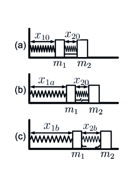
Figure 1: (a) A body with mass $m_{1}$ starts to move from $x_{1}=x_{10}$. A body with mass $m_{2}$ is stuck to the mass body with mass $m_{1}$. (b) When the body with mass $m_{1}$ reaches $x_{1}=x_{1a}$, the spring between the two bodies starts to release. (c) Two bodies position when the body with mass $m_{2}$ has its maximum velocity.

The equations for a two coupled harmonic oscillator are:

$$\left(\begin{array}[]{cc}m_{1}&0\\ 0&m_{2}\end{array}\right)\left(\begin{array}[]{c}x^{{}^{\prime\prime}}_{1}(t)\\ x^{{}^{\prime\prime}}_{2}(t)\end{array}\right)=-\left(\begin{array}[]{cc}k_{1}+k_{2}&-k_{2}\\ -k_{2}&k_{2}\end{array}\right)\left(\begin{array}[]{c}x_{1}(t)\\ x_{2}(t)\end{array}\right),$$

and the eigenvalue equation we have to solve is:

$$\left(\begin{array}[]{cc}\frac{k_{1}+k_{2}}{m_{1}}&-\frac{k_{2}}{m_{1}}\\ -\frac{k_{2}}{m_{2}}&\frac{k_{2}}{m_{2}}\end{array}\right)\left(\begin{array}[]{c}A_{1}\\ A_{2}\end{array}\right)=\omega^{2}\left(\begin{array}[]{c}A_{1}\\ A_{2}\end{array}\right)$$

, where, two eigenvalues $\omega^{+}$ and $\omega^{-}$ are as follow:

$$\omega^{\pm}=\sqrt{\frac{A_{b}\pm A_{a}}{2m_{1}m_{2}}},$$ (1)

The eigenvectors $\lambda^{+}$ and $\lambda^{-}$ for $\omega^{+}$ and $\omega^{-}$ are:

$$\lambda^{\pm} = \left(\begin{array}[]{c}\lambda_{1}^{\pm}\\ \lambda_{2}^{\pm}\end{array}\right)$$ (4)

$$= \left(\begin{array}[]{c}\frac{1}{2k_{2}m_{1}}(-A_{c}\pm A_{a})\\ 1\end{array}\right),$$ (7)

where,

$$A_{a} = \sqrt{(k_{1}m_{2}+k_{2}(m_{1}+m_{2}))^{2}-4k_{1}k_{2}m_{1}m_{2}},$$ (8)

$$A_{b} = k_{1}m_{2}+k_{2}m_{2}+k_{2}m_{1},$$ (9)

$$A_{c} = k_{1}m_{2}+k_{2}m_{2}-k_{2}m_{1}.$$ (10)

Then the solutions of motion become:

$$x_{1}(t) = a_{1}\lambda_{1}^{+}\cos\omega^{+}t+a_{2}\lambda_{1}^{+}\sin\omega^{+}t+b_{1}\lambda_{1}^{-}\cos\omega^{-}t+b_{2}\lambda_{1}^{-}\sin\omega^{-}t,$$

$$x_{2}(t) = a_{1}\lambda_{2}^{+}\cos\omega^{+}t+a_{2}\lambda_{2}^{+}\sin\omega^{+}t+b_{1}\lambda_{2}^{-}\cos\omega^{-}t+b_{2}\lambda_{2}^{-}\sin\omega^{-}t.$$ (11)

If we set the boundary condition at $t=0$, the second body gets its maximum velocity and the velocity of the first body is zero at the equilibrium position. In other words, the initial potential energy is totally converted into the kinetic energy of the second body. For this requirement, the initial conditions should be $x_{1}(0)=0,x_{2}(0)=0,x_{1}^{\prime}(0)=0,x_{2}^{\prime}(0)=v_{0}$. Then the solutions $x_{1}(t),x_{2}(t)$ in Eq. 11 can be written

$$x_{1}(t) = \sqrt{2}k_{2}m_{2}v_{0}(\sqrt{\frac{A_{b}+A_{a}}{m_{1}m_{2}}}\sin[\frac{(A_{b}-A_{a})t}{\sqrt{2}m_{1}m_{2}}]$$

$$-\sqrt{\frac{A_{b}-A_{a}}{m_{1}m_{2}}}\sin[\frac{(A_{b}+A_{a})t}{\sqrt{2}m_{1}m_{2}}])/(\sqrt{A_{a}}\sqrt{\frac{A_{b}-A_{a}}{m_{1}m_{2}}}\sqrt{\frac{A_{b}+A_{a}}{m_{1}m_{2}}}),$$

$$x_{2}(t) = v_{0}((A_{c}+A_{a})(\sqrt{\frac{A_{b}+A_{a}}{m_{1}m_{2}}}\sin[\frac{(A_{b}-A_{a})t}{\sqrt{2}m_{1}m_{2}}]$$ (12)

$$+((A_{a}-A_{c})\sqrt{\frac{A_{b}-A_{a}}{m_{1}m_{2}}}\sin[\frac{(A_{b}+A_{a})t}{\sqrt{2}m_{1}m_{2}}])/(\sqrt{2}A_{a}\sqrt{\frac{A_{b}-A_{a}}{m_{1}m_{2}}}\sqrt{\frac{A_{b}+A_{a}}{m_{1}m_{2}}}),$$

and the velocities $v_{1}(t),v_{2}(t)$ are:

$$v_{1}(t) = k_{2}m_{2}v_{0}(\cos[\frac{\sqrt{A_{b}-A_{a}}}{\sqrt{2m_{1}m_{2}}}t]-\cos[\frac{\sqrt{A_{b}+A_{a}}}{\sqrt{2m_{1}m_{2}}}t])/A_{a},$$

$$v_{2}(t) = v_{0}((A_{c}+A_{a})\cos[\frac{\sqrt{A_{b}-A_{a}}}{\sqrt{2m_{1}m_{2}}}t]$$ (13)

$$+(A_{a}-A_{c})\cos[\frac{\sqrt{A_{b}+A_{a}}}{\sqrt{2m_{1}m_{2}}}t])/(\sqrt{2}A_{a}).$$

Returning to our problem, from these solutions we can find the release time of the second body. First, the second body was stuck to the first body with initial potential energy $\frac{1}{2}k_{2}x_{20}^{2}$; then, at a certain time $t=-\tau$, the second spring starts to play a role, and at time $t=0$, the second body has its maximum kinetic energy. To find the time $t=-\tau$, we set these two velocities in Eq. 13 to be the same.

However, it is impossible to find the general analytic solution for $\tau$ such that $v_{1}(-\tau)$ is equal to $v_{2}(-\tau)$.

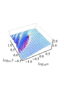
Figure 2: Release time to get an maximum conversion efficiency as a function of $log_{10}\alpha$ and $log_{10}\beta$ , where $\alpha=\frac{m_{1}}{m_{2}}$ and $\beta=\frac{k_{1}}{k_{2}}$

In Fig. 2, we numerically solve these equations and plot the time $\tau$ such that $v_{1}(-\tau)=v_{2}(-\tau)$ as a function of $log_{10}\alpha$ and $log_{10}\beta$ , where $\alpha=\frac{m_{1}}{m_{2}}$ and $\beta=\frac{k_{1}}{k_{2}}$. Although we can’t find the general solution, we get some solutions for the extreme case ,

$$\tau = \sqrt{\frac{m_{1}}{k_{1}+k_{2}}}\arccos[\frac{k_{1}}{k_{2}}],\qquad m2>>m1$$

$$\tau = \sqrt{\frac{m_{2}}{k_{2}}}\frac{\pi}{2},\qquad m1>>m2.$$ (14)

Once, we find the solution for the time $\tau$ such that $V_{A}=v_{1}(-\tau)=v_{2}(-\tau)$ in Eq. 13, we have to find the analytic solutions for the two tied bodies connected to the first spring. In other words, two bodies sticking to each other move at first with the same velocity by the first spring. The contraction length of the second spring can be calculated as follows:

$$\delta x_{2}=x_{2}(-\tau)-x_{1}(-\tau)$$ (15)

The initial starting time and the position of the first body are calculated from the following general equations such that two bodies are attached at the spring with boundary conditions such that $x_{two}(-\tau)=x_{1}(-\tau),v_{two}(-\tau)=V_{A}$, where $x_{two}(t)$ and $v_{tw0}(t)$ are position and the velocity of the two tied body , respectively. The solutions of $x_{two}$ and $v_{two}$ are as follows:

$$x_{two}(t) = x_{1}(-\tau)\cos(\sqrt{\frac{k_{1}}{m_{1}+m_{2}}}(t+\tau)+\sqrt{\frac{m_{1}+m_{2}}{k_{1}}}V_{A}\sin(\sqrt{\frac{k_{1}}{m_{1}+m_{2}}}(t+\tau),$$

$$v_{two}(t) = V_{A}\cos(\sqrt{\frac{k_{1}}{m_{1}+m_{2}}}(t+\tau))-\sqrt{\frac{k_{1}}{m_{1}+m_{2}}}x_{i}\sin(\sqrt{\frac{k_{1}}{m_{1}+m_{2}}(t+\tau}).$$ (16)

The contraction length of the first spring can be obtained using Eq. 16. If we find the time $t=-T_{s}$ such that $v_{two}(-T_{s})=0$, the initial condition of the first spring is $\delta x_{1}=x_{two}(-T_{s})$.

In order to transfer all the potential energy of two springs into the kinetic energy of the second body, we tie the second spring with contraction length $\delta x_{2}$ and let the two bodies move together by the first spring with the initial position $x_{two}(-T_{s})$. After two bodies move together, at $t=-\tau$ we set the second spring release, then the two bodies become a two coupled harmonic oscillator. Then at $t=0$, the kinetic energy of the second body has its maximum value, which is the same as the initial potential energy of the two springs. The scenario is that the kinetic chain process converts the initial potential energy into the kinetic energy of the second body, by controlling the time delay.

To obtain an explicit result, we set the mass of two bodies to be the same ($m_{1}=m_{2}=m=1kg$) and the spring constants are the same ($k_{1}=k_{2}=1N/m$), then the two solutions become:

$$x_{1}(t) = \frac{v_{0}(\sqrt{3+\sqrt{5}}\sin(\sqrt{\frac{1}{2}(3-\sqrt{5})}\omega_{0}t)-\sqrt{3-\sqrt{5}}\sin(\sqrt{\frac{1}{2}(3+\sqrt{5})}\omega_{0}t))}{\sqrt{10}\omega_{0}},$$

$$x_{2}(t) = \frac{1}{2\sqrt{10}\omega_{0}}\{v_{0}((1+\sqrt{5})\sqrt{3+\sqrt{5}}\sin(\sqrt{\frac{1}{2}(3-\sqrt{5})}\omega_{0}t)$$ (17)

$$-\sqrt{3-\sqrt{5}}\sqrt{\sqrt{5}-1}\sin(\sqrt{\frac{1}{2}(3+\sqrt{5})}\omega_{0}t))\}$$

$$v_{1}(t) = \frac{v_{0}(\cos(\sqrt{\frac{1}{2}(3-\sqrt{5})}\omega_{0}t)-\cos(\sqrt{\frac{1}{2}(3+\sqrt{5})}\omega_{0}t))}{\sqrt{5}},$$

$$v_{2}(t) = \frac{v_{0}((1+\sqrt{5})\cos(\sqrt{\frac{1}{2}(3-\sqrt{5})}\omega_{0}t)+\sqrt{\sqrt{5}-1}\cos(\sqrt{\frac{1}{2}(3+\sqrt{5})}\omega_{0}t))}{2\sqrt{5}}.$$ (18)

We obtain the numerical solution for the equation $v_{1}(t)=v_{2}(t)$ in Eq. 18, and the result is $\tau\sim-1.15s$. If we want to obtain the final conditions that the second body has a velocity and a position at $t=0$ such that $v_{2}(0)=1m/s,x_{2}(0)=0$ when the first body has a velocity and a position at $t=0$ such that $v_{1}(0)=0,x_{1}(0)=0$, the two bodies should have the same velocity at $t=-\tau$ such that $v_{1}(-\tau)=v_{2}(-\tau)=0.47m/s$. From Eq. 17, the length of the spring between two bodies at $t=-\tau$ should be $x_{2}(-\tau)-x_{1}(-\tau)=-0.93m-(-0.21)m=-0.72m$. In order to get the velocity $v_{12}(-\tau)=0.47m/s$ for the two tied bodies, we can find the initial time $T_{s}\sim-2.92s$ from Eq. 16. The initial position of the first spring is $x_{s}=x_{two}(-T_{s})\sim-0.69m$.

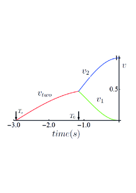
Figure 3: Velocity of two bodies. Two bodies starts to move at $T_{s}=-2.92s$ at the initial position $x_{s}=-0.693m$. The two bodies moves together until $t=T_{d}=-1.15s$, and then the two bodies are separated by the second spring. At $t=0$, the second body has its maximum velocity $v_{2}=1m/s$ at $x_{2}(0)=0$. The velocity of the first body is $v_{1}=0$ at $x_{1}(0)=0$. We assume that $m_{1}=m_{2}=1kg$, and $k_{1}=k_{2}=1N/m$, for simplicity.

In Fig. 3, we plot the velocities of the two bodies. The two bodies start to move at $T_{s}=-2.92s$ at the initial position $x_{s}=-0.69m$. The second body is tied to the first body by the fixed spring, with keeping the relative position between two bodies as $-0.72m$ from the equilibrium position. The two bodies move together until $t=-T_{d}=-1.15s$, and then the two bodies are separated by the second spring as in Fig. 1. At $t=0$, the second body has its maximum velocity $v_{2}=1m/s$ at $x_{2}(0)=0$. The velocity of the first body is $v_{1}=0$ at $x_{1}(0)=0$.

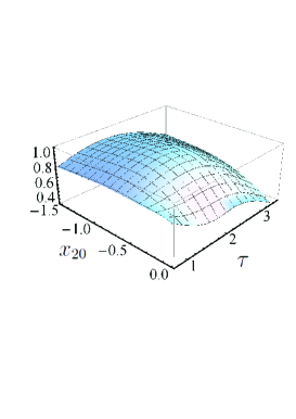
Figure 4: The ratio between the maximum kinetic energy of the body ($m_{2}$) and the initial potential energy stored in two springs. The ratio is shown as a function of the release time $\tau$ and length ($x_{20}$) of the spring between the two bodies.

Up until now, we have found the solution that the initial potential energy stored in the two springs is totally converted to the kinetic energy of the second body at $t=0$. If we change the release time $\tau$ and the potential energy stored in t the second spring $x_{20}$, the kinetic energy of the second body at $t=0$ changes. Figure 4 plots the ratio between the maximum kinetic energy of the second body and the initial potential energy stored in the two springs as a function of the release time $\tau$ and length ($x_{20}$) of the spring between the two bodies. The figure shows that the efficiency is sensitive to the release time. In other words, to get maximum efficiency, we have to very carefully control the release time. The release time is an essential key element in the kinetic chain process. This effect will be discussed in the next section in detail, when we consider the kinetic chain in the three pendulum model.

III The kinetic chain in the Three pendulum model

Figure 5: Triple pendulum model with three massless rods and three point masses. We assume that the forces are only the Hooke’s forces caused by the angles $\theta_{1},\theta_{2},\theta_{3}$ are $-k_{1}\theta_{2}$, $-k_{2}(\theta_{2}-\theta_{1})$ and $-k_{3}(\theta_{3}-\theta_{2})$, respectively.

When we stroke a ball by racket or bat, the system is very complicated and it is not easy to study the system in detail. But in this article, we used the simplest model where we set the body, the forearm and the arm, and the racket as a triple pendulum with massless rod and mass attached at each rod’s end. Figure 5 shows the geometry of the triple pendulum model for the swing of a racket. The triple pendulum is composed of three rods $l_{1},l_{2},l_{3}$ and three masses $m_{1},m_{2},m_{3}$, as in Fig. 5. We assumed that the three rods have no mass, and that the forces applied to the three rods are $-k_{1}\theta_{2}$, $-k_{2}(\theta_{2}-\theta_{1})$ and $-k_{3}(\theta_{3}-\theta_{2})$, respectively, where the three angles are defined as the angle of each rod from the vertical line. Hooke’s forces are surely not a sufficient model for the stroke system, but we used this simple model to study the kinetic chain in this article.

We set the variables as follows:

$$\begin{array}[]{ll}x_{1}(t)=l_{1}\sin\theta_{1},&y_{1}(t)=l_{1}\cos\theta_{1},\\ x_{2}(t)=x_{1}(t)+l_{2}\sin\theta_{2},&y_{2}(t)=y_{1}(t)+l_{2}\cos\theta_{2},\\ x_{3}(t)=x_{2}(t)+l_{3}\sin\theta_{3},&y_{3}(t)=y_{3}(t)+l_{3}\cos\theta_{3},\\ \end{array}$$

Then the kinetic energy ($T$) and the potential energy ($V$) become:

$$T = \frac{1}{2}[l_{1}^{2}(m_{1}+m_{2}+4m_{3})\beta_{3}^{\prime}(t)^{2}+l_{2}^{2}(m_{2}+m_{3})(\beta_{1}^{\prime}(t)+\beta_{3}^{\prime}(t))^{2}$$ (19)

$$+ l_{3}^{2}m_{3}(\beta_{1}^{\prime}(t)+\beta_{2}^{\prime}(t)+\beta_{3}^{\prime}(t))^{2}+4l_{1}l_{3}m_{3}\cos(\beta_{1}(t)+\beta_{2}(t))(\beta_{1}^{\prime}(t)+\beta_{2}^{\prime}(t)+\beta_{3}^{\prime}(t))\beta_{3}^{\prime}(t)$$

$$+ 2l_{2}(\beta_{1}^{\prime}(t)+\beta_{3}^{\prime}(t))\{l_{1}(m_{2}+2m_{3})\cos\beta_{1}(t)\beta_{3}^{\prime}(t)$$

$$+ l_{3}m_{3}\cos\beta_{2}(t)(\beta_{1}^{\prime}(t)+\beta_{2}^{\prime}(t)+\beta_{3}^{\prime}(t))\}],$$

$$V=\frac{1}{2}\{k_{1}\beta_{1}(t)^{2}+k_{2}\beta_{2}(t)^{2}+k_{3}\beta_{3}(t)^{2}\},$$ (20)

where,

$$\beta_{1} = \theta_{2}-\theta_{1},$$

$$\beta_{2} = \theta_{3}-\theta_{2},$$

$$\beta_{3} = \theta_{1}.$$ (21)

Then using the Lagrangian $L=T-V$, we can find the Lagrange Equations for $\beta_{1}(t),~{}\beta_{2}(t),~{}\beta_{3}(t)$, as follows:

$$\frac{d}{dt}\frac{dL}{d\beta_{i}^{\prime}(t)} = \frac{dL}{d\beta_{i}(t)},i=1,2,3$$ (22)

In order to find the efficient method to convert the initial potential energy into the kinetic energy of $m_{3}$ using the kinetic chain process, we follow the same way as in the two coupled springs in section II based on the kinetic chain process. First, we set the initial relative angle of the three rods as $\theta_{10},\theta_{20},\theta_{30}$, then we fix the initial potential energy of this system, and then we set the three pendulum moves. But, at the first stage, we do not release the second ($\theta_{2}$) and the third angle ($\theta_{3}$). With fixing two angles we solve the effective single pendulum. After a certain time $T_{A}$ passes, we release the second angle $\theta_{2}$, while still keeping the third angle $\theta_{3}$ fixed. After passing another time $T_{B}$, we finally release the third angle $\theta_{3}$, and try get the maximum speed of the mass $m_{3}$. We are interested in the time delays $T_{A}$ and $T_{B}$,which are related to the kinetic chain process. However, there are no analytic solutions to get the most efficient method to maximize the angular speed of the third rods under the given initial potential energy.

As in Section II, we start to find the solution by the time reversal method. At time $t=0$, we set the boundary conditions that the potential energy is totally converted into the kinetic energy of $m_{3}$. We try to numerically solve the differential equations in Eq. 22 with the boundary conditions of:

$$\beta_{1}(0) = \beta_{2}(0)=\beta_{3}(0)=0,$$

$$\beta_{1}^{\prime}(0) = \beta_{3}^{\prime}(0)=0,$$

$$\beta_{2}^{\prime}(0) = \dot{\theta}_{3}.$$ (23)

In our simulation, the third rod with mass $m_{3}$ reaches its maximum angular velocity $\dot{\theta}_{30}$ at $t=0$ when the third rod arrives at $\theta_{3}(0)=0$. The other two rods arrive at the equilibrium positions $\theta_{1}(0)=\theta_{2}(0)=0$ with angular velocity zero. At this stage, we study the time behavior of the three rods retrospectively and we have to find the time ($T_{A}$) when the angular velocities of the second rod and the third rod are the same, as follows:

$$\theta_{2}^{\prime}(-T_{A})=\theta_{3}^{\prime}(-T_{A}).$$ (24)

If we find the time $T_{A}$, we set new equations for $\beta_{1}(t),~{}\beta_{3}(t)$ from Eq. 22 with replacement $\beta_{2}^{\prime}(t)=0$ and $\beta_{2}(t)=\beta_{2}(-T_{A})$. Then the solution is for the double pendulum, the first pendulum is for the first rod and the second pendulum is for the two rods whose relative angle is fixed. When $t<-T_{A}$, the second rod and the third rod move together with the angle between them fixed as $\beta_{2}(-T_{A})$. At $t=-T_{A}$, the third rod starts to release from the second rod and it starts to move and reaches its maximum velocity at $t=0$.

Before the time that the third rod releases at $t=-T_{A}$, the second and the third rod move together. Now we have to find the release time of these two rods from the first rod. The time can be obtained from the following conditions

$$\theta_{2}^{\prime}(-T_{B})=\theta_{1}^{\prime}(-T_{B}).$$ (25)

If we find the time $T_{B}$, we set new equations for $\beta_{3}(t)$ from Eq. 22 with replacement $\beta_{2}^{\prime}(t)=0,\beta_{1}^{\prime}(t)=0$ and $\beta_{2}(t)=\beta_{2}(-T_{A}),\beta_{1}(t)=\beta_{1}(-T_{B})$. Then the solution is for the effective single pendulum, and the relative angles among the three rods are fixed. When $t<-T_{B}$, the three rods move together with the angles among them being $\beta_{2}(-T_{A}),\beta_{1}(-T_{B})$. At $t=-T_{B}$, the tied second rod and the third rod start to release from the first rod. We can also find the start time of the effective single pendulum by solving these equations,

$$\theta_{3}^{\prime}(-T_{S})=0.$$ (26)

If we follow the time series sequentially from $t=-T_{s}$, we can see clearly the kinetic chain process. At first the angles among the three rods are fixed, the initial angle of the first rod is $\theta_{10}=\beta_{3}(-T_{S})$ and three rods starts to move together until $t=-T_{B}$. At $t=-T_{B}$, the second rod release from the first rod with keeping the angle between the second and the third rod until $t=-T_{A}$. At $t=-T_{A}$, the third rod releases from the second rod and the third rod starts to release from the second rod, starts to move, and reaches its maximum velocity at $t=0$.

To get an explicit result, we assume the mass and length of the pendulum. We assume that the masses of the three bodies are $m_{1}=10kg$, $m_{2}=3kg$, $m_{3}=0.2kg$ and the lengths of the three rods are $l_{1}=0.3m$, $l_{2}=0.5m$, and $l_{3}=0.75m$. These values come from one example of the body, forearm and arm, and racket system. We also assume that the spring constants of the three rods are $k_{1}=5N/m$, $k_{2}=1N/m$, and $k_{3}=0.25N/m$. Although these numerical values are not actual data, we can study the role of the kinetic chain based on these particular examples.

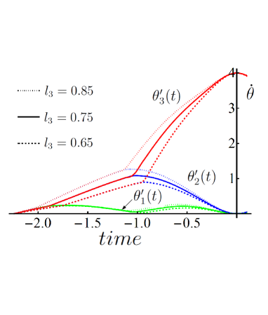
Figure 6: Angular velocities of three rods. At first two rods are moves with the same angular velocity. After a short time ($T_{1}$), the second rod starts to move together with the third rods. Finally at time $T_{2}$, the third rod independently starts to move. At $t=0$, the third rods gets maximum angular velocity as the other two rods have zero angular velocities at equilibrium.

Figure 6 shows the angular velocities of three rods with the particular example. First, the three rods move together with the initial angle $\theta_{1}=18.3^{\circ}$ at $t=-2.24s$, until $t=-1.89s$. At $t=-1.89s$, the second rod is released from the first rod. The initial relative angle between the first and the second rod is $52.7^{\circ}$. The angular velocity of the first rod is decreased after releasing the second rod. The angular velocity of the second rod is increased till $t=-1.04s$. Until then, the third rod is attached to the second rod, and the two rods move together. After $t=-1.04s$, the three rods move separately, and the initial relative angle between the second and the third rod is $132.9^{\circ}$. The angular velocity of the first rod is increased a little, and the angular velocity of the second rod is decreased. Only the angular velocity of the third rod is increased, and reaches the maximum velocity at $t=0$. All the potential energy is converted into the kinetic energy of the third rod, which is the truly perfect kinetic chain process.

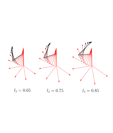
Figure 7: The traces of three pendulums for different length $l_{3}$ with keeping other conditions unchanged. The shots are taken at equal time intervals from the starting time. As the length $l_{3}$ increases the initial angle of the third rod should increase. The red lines are under the force, and the black lines remain fixed without generating Hooke’s force.

Figure 7 shows the traces of the three pendulum from the time $t=-2.24s$, till $t=0.25s$ with equal time interval for $l_{3}=0.65m,~{}0.75m,~{}0.85m$. The red line represents the released rod and the black line represent the fixed rods. For the pendulum with $l_{3}=0.75m$, at first the second and the third rods are fixed, and the pendulum moves using the potential energy stored at the first rod, until $t=-1.89s$ (two steps in our figure). After $t=-1.89s$, the second rod is released and moves together with the third rod till $t=-1.04s$ (four steps in our figure). After that, the three rods move separately, and the third rod gets its maximum angular velocity at $t=0$. The start time for different $l_{3}$ is almost the same, but the initial starting angle $\theta_{1}$ is increased as $l_{3}$ increases in Fig. 7. The initial angle is also increased as $l_{3}$ changes from $l_{3}=0.65m$ to $l_{3}=0.85m$. The maximum angular velocity of the third rod at $t=0$ is initially set to $\dot{\theta_{3}}=4rad/s$, but the linear velocity is increased as $l_{3}$ increases. All the potential energy is converted into the kinetic energy of the third rod and the kinetic energy is also increased for large $l_{3}$, which is why the initial angle should be increased to get large kinetic energy. The most important thing in the kinetic chain process is the release time. Figure 6 shows the change of the release time for different $l_{3}$. Considering the longer triple pendulum with $l_{3}=0.85m$, the angular velocity of the second rod just before releasing the third rod is greater than the shorter triple pendulum with $l_{3}=0.65m$. The releasing time for the third rod of the longer triple pendulum is earlier than that of the shorter triple pendulum. If we check the time from $t=0$, the acceleration time for the shorter triple pendulum is shorter than that of the longer triple pendulum.

Figure 8 shows the effect of changing the third body. For the lighter triple pendulum with $m_{3}=0.2kg$, the initial relative angles among three rods is smaller than those for the heavier triple pendulum with $m_{3}=0.4kg$. The trend is almost same considering the shorter and longer triple pendulum. The reason is related to the kinetic energy of the third rod at $t=0$. In our simulation, we fixed the angular velocity of the third rod as $\dot{\theta_{3}}=4rad/s$, but the kinetic energy of the third rod is $\frac{1}{2}m_{3}(l_{3}\dot{\theta_{3}})^{2}$, and the kinetic energy comes from the potential energy which is a function of the three relative angles among the three rods.

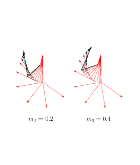
Figure 8: The traces of three pendulums for different mass $m_{3}$ with keeping other conditions unchanged. The shots are taken at equal time interval from the starting time. As the length $m_{3}$ increases the initial angle of the third rod should be increased. The red rods are under the force and the black rods remain fixed without generating Hooke’s force.

Figure 9 shows the maximum velocity of the third rod as a function of the release times $T_{A}$ and $T_{R}$, where $T_{A}$ is the holding time for the second and the third rod, and $T_{R}$ is the holding time for the third rod. For the original triple pendulum, $T_{A}=-1.89s-(-2.24)s=0.35s$, and $T_{R}=-1.04s-(-1.89)s=0.85s$. As shown in Fig. 9, the maximum velocity cannot be increased as $T_{A}$ and $T_{R}$ changes from the value $T_{A}=0.35s$ and $T_{B}=0.85s$. That is simply because the condition we found is the most efficient condition in which the initial potential energy is totally converted into the kinetic energy of the third rod. We can only see how fast the maximum velocity changes as the release times change.

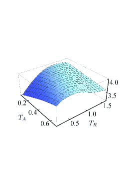
Figure 9: The maximum angular velocity of the third rod as a function of the release times $T_{A}$ and $T_{R}$, where $T_{A}$ is the holding time for the second rod, and $T_{R}$ is the holding time for the third rod

We also find the condition that the initial relative angles among three rods for a given angular velocity of the third rod as a function of $m_{3}$ and $l_{3}$.

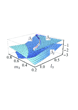
Figure 10: Initial angle of $\beta_{1}$, $\beta_{2}$, $\beta_{3}$ as a function of the mass of the third body($m_{3}$) and length of the third rod($l_{3}$).

The upper-most surface legend by $\beta_{3}$ is the initial angle of the first rod. But $\beta_{3}$ has no negative solutions for the entire $m_{3}$ and $l_{3}$ space in Fig. 9. For a small $l_{3}=0.5m$, the initial angle $\beta_{3}$ has solutions for $0.2kg<m_{3}<0.7kg$, but as $l_{3}$ increases, the initial angle $\beta_{3}$ has solutions for light mass. Actually there are some solutions for positive $\beta_{3}$. In other words, the triple pendulum starts to moves initially from positive $\beta_{3}$ and goes back to the negative angle with negative angular velocity then returns to the original direction with positive angular velocity. For a given length $l_{3}$, the initial relative angle $\beta_{2}$ decreases as $m_{3}$ decreases, but the initial relative angle $\beta_{1}$ increases as $m_{3}$ decreases. For a given mass $m_{3}$, the initial relative angle $\beta_{1}$ increases as $l_{3}$ increases, but the dependence of the initial relative angle $\beta_{2}$ is complex, $\beta_{2}$ increases for light $m_{3}$ and $\beta_{2}$ decreases and finally increases for heavy $m_{3}$. Until now we have studied the kinetic chain process that transfers initial potential energy into the kinetic energy of the third body using proper time delays. Controlling the time sequence in a triple pendulum is an essential element to make a perfect kinetic chain process until now.

IV Triple pendulum without time delay

Section III, the springs between rods are not simultaneously released, but in proper time sequence in order to make a perfect kinetic chain process. However, if we want to transfer all the potential energy to the kinetic energy of the third rod, another solution can be found. Figure 11 shows the solution, where we plot the angular velocities of the three rods. The three rods start to move without any time lag from the beginning. At first, the angular velocities of the first and the second rod are zero, and the angular velocity of the third rod is negative. The initial angles of the three angles are $\theta_{1}=-6.8^{\circ}$, $\theta_{2}=-20.0^{\circ}$, $\theta_{3}=-8.7^{\circ}$. The first and the second rods move forward, and the angular velocities increase at first, and then go to zero at $t=0$. On the other hand, the third rod starts to move backward, and turns its direction. The final velocity of the third rod is $\dot{\theta_{3}}=0.93rad/s$. If we consider the kinetic chain as a mechanism that efficiently transfers the potential energy into kinetic energy, the kinetic chain we found here does not require a time lag. The difference from the result in Section III is the initial condition. In Section III, the initial conditions for the three angular velocities are zero. If we release these restrictions, we have a new solution as in Fig. 11, where the initial angular velocity of the third rod is not zero, but has a negative value. At $t=0$, the angular velocity of the third rod is less than $1rad/s$, which is smaller than $4rad/s$. Actually there is no systematic process for arbitrary $\dot{\theta_{3}}$. On the contrary, in Section III, we can systematically find the initial conditions that gives perfect energy transfer for a given $\dot{\theta_{3}}$.

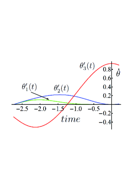
Figure 11: Angular velocities of the three rods. The three rods move from the beginning without delay, the initial angular velocities of the first and the second rod are zero and the initial angular velocity of the third rod is negative. As time passes, the angular velocity of the third body changes, and it has its maximum $\dot{\theta_{3}}=0.93rad/s$ at $t=0$.

In order to increase the angular velocity of the third rod, we try to find new solution using a minimizing algorithm. In Fig. 12, the final angular velocity of the third rod is $\dot{\theta_{3}}=2.0rad/s$. But the initial angular velocities of the two rods are not exactly zero, the angular velocities are $\dot{\theta_{1}}(0)=-0.03rad/s$ and $\dot{\theta_{2}}(0)=-0.09rad/s$, respectively. First, the angular velocity of the first rod reaches its maximum, and decreases to zero, and at that time, the angular velocity of the second rod gets its maximum velocity. When the angular acceleration of the second rod turns to negative, the angular velocity of the third rod changes from negative value to positive velocity. At $t=0$, the rod obtains the maximum value $\dot{\theta_{3}}=2.0rad/s$, and the angular velocities of the first and the second rod are zero.

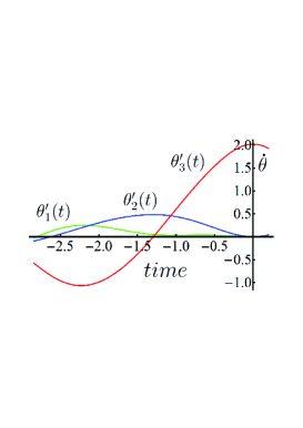
Figure 12: Angular velocities of the three rods. The three rods move from the beginning without delay, the initial angular velocities of the first and the second rod are almost zero, and the initial angular velocity of the third rod is negative. As time passes, the angular velocity of the third body changes, and it has its maximum $\dot{\theta_{3}}=2.0$ at $t=0$.

Figure 13 shows the trajectory of the three rods from the time beginning until the contact time. At the first shot (1) in Fig. 13, the initial angles of three rods are $\theta_{1}=-15.7^{\circ}$, $\theta_{2}=-41.3^{\circ}$ $\theta_{1}=-20.9^{\circ}$, respectively. As shown in this figure, the third rod moves backward from the first shots to the sixth shot(1-6). After the seventh shot the third rod rapidly moves forward and has its maximum angular velocity on the 11th shot at $t=0$. At $t=0$, the angles of the three rods are all zero.

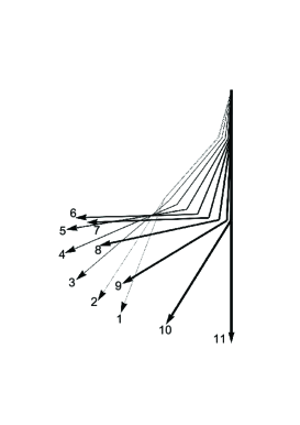
Figure 13: The trajectory of the three rods from the beginning time until the contact time. The third rod moves backward from the first shot to the sixth shot. After the seventh shot the third rod rapidly moves forward, and has its maximum angular velocity at the 11th shot.

If we set the initial condition that the three angular velocities are all the same, there can be another solution that gives efficient energy transfer. The initial angular velocities of the three rods are $\dot{\theta_{1}}(0)=\dot{\theta_{2}}(0)=\dot{\theta_{3}}(0)=-0.2rad/s$, respectively. In this case, yhr three rods in the triple pendulum first move together with the same angular velocity. As in Fig. 14, first the angular velocity of the first rod changes from the negative to the positive, and decreases to be zero, and the angular velocity of the second rod also changes from negative to positive and reaches its maximum velocity. When the angular acceleration of the second rod turns to negative, the angular velocity of the third rod changes from the negative value to the positive velocity. At $t=0$, the angular velocity of the third rod reaches the maximum value $\dot{\theta_{3}}=2.0rad/s$, and the angular velocities of the first and the second rod are zero.

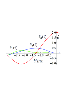
Figure 14: Angular velocities of the three rods. The three rods move from the beginning without delay, the initial angular velocities of the three rods are the same and negative. After a short time, the angular velocities of the first and the second rod change into positive value. The third rod moves backward, changes its direction, and get its maximum angular velocity $\dot{\theta_{3}}=2.0$ at $t=0$.

Figure 15 shows the trajectory of the three rods from the beginning time until the contact time. At the first shot (1) in Fig. 15, the initial angles of the three rods are $\theta_{1}=-14.0^{\circ}$, $\theta_{2}=-39.0^{\circ}$, $\theta_{3}=-14.9^{\circ}$, respectively. As shown in this figure, the third rod moves backward from the first shot to the sixth shot(1-6). After the seventh shot, the third rods rapidly moves forward, and has its maximum angular velocity at the 11th shot at $t=0$. At $t=0$, the angles of the three rods are all zero.

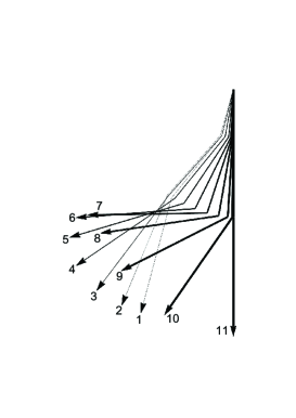
Figure 15: The trajectory of the three rods from the time beginning till the contact time. As shown in this figure, the three rods moves backward at first. The first and the second rod moves to back ward till the second shot and they start to move forward from the third shot. The third rod moves backward till the seventh shot, and it begin to move forward and has its maximum angular velocity at the 11th shot.

In this section, we introduced a new method to transfer initial energy including the potential energy of three bodies in a triple pendulum into the kinetic energy of the third body on the third rod. This method does not require a time delay which is essential in a kinetic chain process.

V Conclusion and Discussion.

The pendulum model is applied to baseball, tennis, and golf. In particular, the swing pattern using the double pendulum was studied to maximize the angular velocity of a hitting rod, such as a racket, bat, or club. The time-lagged torque effect for the double pendulum system was studied, and the speed of the rebound ball can be increased not by applying time-independent constant torques on the first rod and the second rod, but by holding the racket for a short time without enforcing a torque and with subsequent application of torque. This mechanism is related to the well known kinetic chain process in a swing pattern system.

In this article, we show the most efficient way to transfer input potential energy to the kinetic energy of a racket or bat based on the kinetic chain process. Introducing the kinetic chain process, we first studied a two coupled harmonic oscillator at first. We analytically showed the method to find the most efficient way to convert the initial potential energy stored in two springs into the kinetic energy of the second body. After releasing the first spring, the two bodies are fix together for the time being. Then the two bodies move together with a fixed distance between them for a short time $\tau$. At $t=\tau$, we release the second spring, then the second body absorbs extra kinetic energy from the second spring. Controlling the initial distance of the two springs and $\tau$, the potential energy initially stored in the two springs can be totally converted into the kinetic energy of the second body. We showed how to find the release time $\tau$ and the initially pressed distance of the two springs, in order to get the most efficiently converted kinetic energy. This method is the most efficient kinetic chain process in a two coupled harmonic oscillator.

We showed how to numerically find the most efficient way to transfer the initial potential energy into the kinetic energy of the third mass. We assumed the force on the triple pendulum is only the Hooke’s force related to the relative angles between the rods, as in Fig. 5. Setting the initial angles of the three rods, we can find the most efficient way to transfer the initial potential energy into the kinetic energy of the third body on the third rod by adjusting the release times $T_{A}$ and $T_{B}$. We are especially interested in the length of the third rod and the mass of the third rod, which are related to the racket system. The racket system may change if we use different rackets or bats or golf clubs. Although our numerical data are not well matched to an actual system, the trend can be applied.

In the kinetic chain process, we usually point out the sequential application of torque or force for each rod in a multiple pendulum model. However, there is a new method that gives perfect energy transfer from the initial conditions into the kinetic energy of the third body on the third rod in a triple pendulum system. The new method did not use the sequential time delays that are essential in a kinetic chain process. However, if we plot the time dependent angular velocities of three bodies as in Figs. 11, 12, 14, the trend of the angular velocities of the first and the second bodies are the same as the result in Fig. 6. As the angular velocity of the first rod decreases, the velocity of the second rod increases. However, the trend of the angular velocity of the third rod is totally different. In the new method in Section IV, the angular velocity of the third body is negative at first, then after the acceleration of the second rod becomes negative, the angular velocity of the third body changes sign. Finally the velocity of the third rod reaches its maximum when the angular velocities of the other rods are zero.

Of course, we used a simple pendulum model with only Hooke’s force, so the results are not directly applicable to the actual swing process using a racket, bat, or golf club. However, we systematically showed how to find the most efficient way to transfer initial potential energy to the kinetic energy of the third rod in a kinetic chain process. Furthermore, we showed an new method to transfer the initial energy to the final kinetic energy without a time lagged process, which is required in a kinetic chain process.

In av actual stroke process, the motion occurs in three dimensions and the magnitudes of the forces and torques depend on the muscle shape and movement. We did not include any bio-mechanical information such as pronation. The numerical data may also not be suitable for some players. However, our study on the kinetic chain process using a triple pendulum system for a stroke provides some insights into attaining an efficient way to transfer body energy to a stroked ball.

References

- (1) D. Williams, Quart. J. Mech. Appl. Math. 20, 247 (1967).
- (2) C. B. Daish, The Physics of Ball Games . (English University Press, London, 1972).
- (3) T. Jorgensen, Am. J. Phys. 38, 644 (1970).
- (4) T. Jorgensen, The Physics of Golf, 2nd ed. (Springer-Verlag, New York, 1999).
- (5) R. Cross, Am. J. Phys. 73, 330 (2005).
- (6) R. Cross, Am. J. Phys. 79, 470 (2011).
- (7) S. Youn, J. Phys. Soc. Kor. 67, 1110 (2015).
- (8) J. Bunn, Scientific Principles of Coaching. (Prentice-Hall,Englewood Cliffs NJ, 1972)
- (9) V. M. Zatsiorsky, Biomechanics in Sport (Blackwell Science,Oxford, 2000)
- (10) J. Landlinger et. al., Journal of Sports Science and Medicine 9, 643-651 (2010).
- (11) JB. Elliott, R. Marshall, G. Noffal, Journal of Sports Science 14, 159-165 (1996).
- (12) A. Ahmadi, et. al., Digital Sport for Performance Enhancement and Competitive Evolution: Intelligent Gaming Technology. 101-121, (2009)
- (13) B. B. Kental, et. al., Journal of Applied Biomechanics, 27, 345-354, (2011)
- (14) M. Sweeney, M. Reid, B. Elliott, Asian Journal of Exercise & Sports Science 9, 13-20(2012).
- (15) R. Cross, Am. J. Phys. 67, 692 (1999).
- (16) R. Cross, Sports Engineering, 6, 235 (2003).
- (17) R. Cross, Am. J. Phys. 68, 1025 (2000).