An Empirical Fitting Method for Type Ia Supernova Light Curves: A Case Study of SN 2011fe

Abstract

We present a new empirical fitting method for the optical light curves of Type Ia supernovae (SNe Ia). We find that a variant broken-power-law function provides a good fit, with the simple assumption that the optical emission is approximately the blackbody emission of the expanding fireball. This function is mathematically analytic and is derived directly from the photospheric velocity evolution. When deriving the function, we assume that both the blackbody temperature and photospheric velocity are constant, but the final function is able to accommodate these changes during the fitting procedure. Applying it to the case study of SN 2011fe gives a surprisingly good fit that can describe the light curves from the first-light time to a few weeks after peak brightness, as well as over a large range of fluxes ($\sim 5$  mag, and even $\sim 7$ mag in the $g$ band). Since SNe Ia share similar light-curve shapes, this fitting method has the potential to fit most other SNe Ia and characterize their properties in large statistical samples such as those already gathered and in the near future as new facilities become available.

1. Introduction

Type Ia supernovae (SNe Ia) are believed to be thermonuclear runaway explosions of carbon/oxygen white dwarfs (see, e.g., Hillebrandt & Niemeyer 2000 for a review). Observationally, SNe Ia share similar light-curve shapes; thus, traditionally the fitting of SN Ia light curves is conducted with templates constructed from well-observed SNe Ia (e.g., Jha et al. 2007; Guy et al. 2007). Some other attempts have also been proposed to characterize SN Ia light curves with different techniques. For example, Kessler et al. (2010) use the Supernova Photometric Classification Challenge, a publicly released tool with simulated SNe for light-curve classification of SNe and photometric redshift estimation; Bazin et al. (2011) employ the SALT2 package (described by Guy et al. 2010) as a SN Ia light-curve fitter to select SN-like events through the photometric sample of the CFHT Supernova Legacy Survey; and Kim et al. (2013) model SN light curves by training a parameterized model for the multiband light curves as arising from a Gaussian process, followed by applying the results to spectrophotometric time series of SNe to simultaneously standardize SNe and fit cosmological parameters. However, to date, no single functional form has been proposed with reasonable physical meaning to fit the light curves of SNe Ia from explosion to a few weeks after peak brightness. In this paper, we present an empirical fitting method to characterize the optical light curves of SNe Ia by using a mathematically analytic function.

2. Fitting Method

SNe Ia are expected to have a “dark phase” which lasts for a few hours to days between the moment of explosion and the first observed light (e.g., Rabinak, Livne, & Waxman 2012; Piro & Nakar 2013, 2014). The “dark phase” could be caused by the varying distribution of ⁵⁶Ni near the surface of a SN Ia. Such evidence is found in SN 2011fe (Piro & Nakar 2013; Mazzali et al. 2014) as well as several other SNe Ia (Hachinger et al. 2013; Shappee et al. 2015; Cao et al. 2016). Hence, the quantity we determine from the data is actually the first-light time ($t_{0f}$) rather than the true explosion time ($t_{0}$). In what follows, however, we do not distinguish between the two; in other words, $t_{0f}\approx t_{0}$, and for simplicity we regard $t_{0}$ as the first-light time in our equations.

Assuming the SN Ia bolometric luminosity scales as the surface area of the expanding fireball (which is approximately a blackbody at early times, modified to some degree by line blanketing in the blue and ultraviolet), and given that optical wavelengths are on the Rayleigh-Jeans tail of its nearly thermal spectral energy distribution at typical temperatures exceeding $\sim 10,000$ K (see §3.3), the optical luminosity of the SN increases quadratically with the photospheric radius (see Riess et al. 1999):

$$L_{\rm opt}\propto R^{2}T\propto[v(t-t_{0})]^{2}T,$$ (1)

where $R$ is the photospheric radius, $T$ is the fireball temperature, $v$ is the photospheric expansion velocity, $t_{0}$ is the first-light time, and $t-t_{0}$ is the time after first light. Assuming that the blackbody temperature is roughly constant at early times (see discussion below), the optical luminosity is

$$L\propto v^{2}(t-t_{0})^{2}.$$ (2)

Thus, considering only very early times (a few days after first light), the optical luminosity should be roughly proportional to the square of the time since first light ($L\propto(t-t_{0})^{2}$, commonly known as the $t^{2}$ model; e.g., Arnett 1982; Riess et al. 1999), assuming the photospheric velocity does not change much. (Note that so far, we have assumed that both the blackbody temperature and the photospheric velocity are constant; both issues will be discussed below.) Observationally, the $t^{2}$ model fits well for several SNe Ia with early-time observations (e.g., SN 2011fe, Nugent et al. 2011; SN 2012ht, Yamanaka et al. 2014).

However, here we aim to extend the fitting to much longer times for SNe Ia (several weeks after first light but before entering the phase dominated by cobalt decay), so it is inappropriate to assume that the photospheric velocity is nearly constant; in fact, observed spectral series show that $v$ drops rapidly at early times and thereafter slowly but steadily decreases (e.g., Silverman et al. 2012). Therefore, a model for the photospheric velocity evolution is required before fitting the light curves of SNe Ia.

Zheng et al. (2017) propose a broken-power-law model to fit the photospheric velocity evolution from the first-light time to more than a month later. The function, which is also widely used for fitting gamma-ray burst afterglows as well as early-time SN Ia light curves (e.g., Zheng et al. 2012; 2013; 2014), is given by

$$v=A\left(\frac{t-t_{0}}{t_{b}}\right)^{\alpha_{1}}\Big{[}1+\left(\frac{t-t_{0}}{t_{b}}\right)^{s({\alpha}_{1}-{\alpha}_{2})}\Big{]}^{-1/s},$$ (3)

where $v$ is the photospheric velocity, $A$ is a scaling constant, $t_{b}$ is the break time, ${\alpha}_{1}$ and ${\alpha}_{2}$ are the two power-law indices before and after the break (respectively), and $s$ is a smoothing parameter. Applying this velocity function to Equation 2, we find the SN Ia optical luminosity to be

$$L=A^{\prime}\left(\frac{t-t_{0}}{t_{b}}\right)^{2(\alpha_{1}+1)}\Big{[}1+\left(\frac{t-t_{0}}{t_{b}}\right)^{s({\alpha}_{1}-{\alpha}_{2})}\Big{]}^{-2/s}.$$ (4)

To simplify this, we introduce $\alpha_{r}$ and ${\alpha}_{d}$ as

$$\alpha_{r}=2(\alpha_{1}+1),$$ (5)

$${\alpha}_{d}={\alpha}_{1}-{\alpha}_{2},$$ (6)

and so Equation 4 becomes

$$L=A^{\prime}\left(\frac{t-t_{0}}{t_{b}}\right)^{\alpha_{r}}\Big{[}1+\left(\frac{t-t_{0}}{t_{b}}\right)^{s{\alpha}_{d}}\Big{]}^{-2/s}.$$ (7)

Equation 7 is the final function we propose to fit to SN Ia light curves for a wide time range (from first light to more than a month later). It reaches a peak value when

$$t_{p}=t_{b}\times(-\frac{\alpha_{1}+1}{\alpha_{2}+1})^{1/[s(\alpha_{1}-\alpha_{2})]}.$$ (8)

The functional form of Equation 7 is very similar to the broken power-law function Equation 3, but with some variance. An advantage of the empirical Equation 7 is that there is reasonable physics behind it; $\alpha_{r}$ is considered the rising power-law index and ${\alpha}_{d}$ the decaying index, and both are related to the photospheric velocity evolution. The function itself is also mathematically analytic, derived directly from the photospheric velocity evolution function (along with the simple assumption that the emission is approximately that of a blackbody).

3. Fitting of SN 2011fe

We choose SN 2011fe as a case study to apply our fitting method; it is the most ideal object for our purpose. First, it was discovered when extremely young and the first-light time is well constrained (Nugent et al. 2011; Li et al. 2011). Second, SN 2011fe is well observed both spectroscopically and photometrically in multiple bands after discovery (e.g., Nugent et al. 2011; Richmond & Smith 2002; Vinko et al. 2012).

3.1. Photospheric Velocity Fitting

Since the fitting function of Equation 7 is derived directly from the photospheric velocity evolution function, we first apply the velocity fitting of SN 2011fe using Equation 3, similar to the fitting of other SNe given by Zheng et al. (2017). Our results are shown in Figure 1, where the photospheric velocity is derived from the strong Si II $\lambda$6355 absorption line.

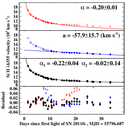
Figure 1.— Photospheric velocity (measured from Si II $\lambda$6355 absorption) evolution of SN 2011fe. Top panel: the result of a power-law fit to the early-time data. Middle-top panel: the result of a linear fit to the later-time data. Middle-bottom panel: the result of a broken power-law fit to all the data. Bottom panel: the residuals for each fit. Solid points are included in the fitting while open points are not.

Figure 1 confirms the finding of Zheng et al. (2017) that the photospheric velocity can be well described by a broken-power-law model (Equation 3) over a relatively long time range. A single power law (top panel) or a linear function (middle-top panel) can fit only either early-time data or later-time data independently, while a broken power law can fit all the data (middle-bottom panel). The single power-law fit at early times gives an index of -0.20, and the single linear function at later times yields $dv/dt=-58$ km s^-1 day^-1, while the composite fit gives power-law indices $\alpha_{1}=-0.22$ and $\alpha_{2}=-0.02$. These results are consistent with the fits to the other SNe Ia (SNe 2009ig, 2012cg, 2013dy and 2016coj) given by Zheng et al. (2017).

3.2. Multiband Light-Curve Fitting

Next, we apply multiband light-curve fitting to SN 2011fe using Equation 7. Optical data are gathered from the published literature (Nugent et al. 2011; Richmond & Smith 2002; Vinko et al. 2012), excluding a few clear $>3\sigma$ outliers among different instruments. Since the light curves of SNe Ia evolve differently in various filters, we fit each monochromatic filter separately. For example, SNe Ia usually exhibit a shoulder in the $R$ band and a second peak in the $I$ band, so we restrict the fits to earlier times in the redder bands ($R$, $I$) than in the bluer bands ($g$, $B$, $V$). Given that the first-light time of SN 2011fe is well estimated (Nugent et al. 2011), we fix $t_{0}$ in the fits. For SN 2011fe, we denote $t_{0}\approx t_{0f}=$ MJD 55,796.687. The fitting results are given in Figure 2 and Table 1.

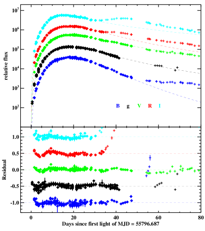
Figure 2.— Multiband light-curve fitting of SN 2011fe using Equation 7, with $t_{0}$ fixed to be $t_{0f}$ (MJD 55,796.687). Diamond-shaped data points are included in the fit while cross-shaped ones are excluded. The fitting results cover both a long time range (from first light to a few weeks after peak time) and a large flux scale (nearly a factor of 100, or $\sim 5$ mag, and even $\sim 7$ mag in $g$).

As shown in Figure 2, by using just a single function (Equation 7), the fitting results are surprisingly good over many weeks and nearly a factor of 100 in flux ($\sim 5$ mag – but $\sim 7$ mag in $g$ where we have extra data from the night of discovery). Most flux residuals are within the 1–2$\sigma$ measurement uncertainty. The fit was applied to a long time range for all filters: for the $g$, $B$, and $V$ bands, data are used up to 50 days after first light, while $R$ (35 days) and $I$ (31 days) are affected by the shoulder and second peak (respectively) in the light curves. Interestingly, although we include data only up to 50 days in $V$, the model still provides a good match the data up to about 3 months post-explosion (though this might be just a coincidence).

The $\alpha_{r}$ values derived from the fits (Table 1) are all around 2.1 (except for $B$, with a somewhat larger value but also more uncertain), close to the $g$-band rising index of 2.01 derived by Nugent et al. (2011) from the first few days of data – though Zhang et al. (2015) find the SN 2011fe rising index to vary from 2.25 to 2.63 in different filters. In general, a rising index around 2.1 is consistent with the commonly known $t^{2}$ model for most SNe Ia, or the $t^{n}$ model ($n\approx 1.5$–3.0) used by various groups (e.g., Conley et al. 2006; Hayden et al. 2010; Ganeshalingam et al. 2011; Firth et al. 2015); however, these previous studies derived the index from the very early-time data (a few days after first-light time), whereas here we derive it from light-curve fitting over a long time using Equation 7.

The other parameters for each filter are also listed in Table 1, but unlike $\alpha_{r}$, they have larger differences among filters. This is not surprising, since the light curves of SNe Ia evolve differently in various filters, especially after peak when the ejecta become optically thinner. However, there is still the possibility of simultaneously fitting all filtered data with the same values of $t_{0}$ (actually $t_{0f}$) and $\alpha_{r}$, since these two parameters can be the same among filters.

Table 1Light-curve fitting results for SN 2011fe, Equation 7

Filter	$\alpha_{r}$ ($\alpha_{1}$)	$t_{b}$	$\alpha_{2}$	$s$
$g$	2.08$\pm$0.02 (0.04$\pm$0.01)	21.2$\pm$1.1	-2.60$\pm$0.12	1.26$\pm$0.12
$B$	2.36$\pm$0.08 (0.18$\pm$0.04)	25.1$\pm$1.4	-4.01$\pm$0.19	0.68$\pm$0.13
$V$	2.10$\pm$0.02 (0.05$\pm$0.01)	19.5$\pm$1.1	-2.19$\pm$0.12	1.57$\pm$0.14
$R$	2.10$\pm$0.02 (0.05$\pm$0.01)	20.4$\pm$1.4	-2.52$\pm$0.17	1.29$\pm$0.17
$I$	2.20$\pm$0.04 (0.10$\pm$0.02)	14.7$\pm$2.0	-1.89$\pm$0.15	2.04$\pm$0.24

3.3. Implications of Parameters

Overall, the fits to the light curves (up to $\gtrsim 1$ month after first light) for SN 2011fe with a single empirical function are very successful. Since SNe Ia share similar light-curve shapes, Equation 7 also has the potential to fit most other SNe Ia. Thus, it is important to understand the possible physics behind this expression.

The form of Equation 7 is a variant of a broken-power-law function. The parameters $A^{\prime}$, $t_{0}$, and $t_{b}$ are easy to understand, while the parameters $\alpha_{r}$, $\alpha_{d}$, and $s$ are inherited from Equation 3, the photospheric velocity evolution function. Here, $\alpha_{r}$ represents the rising power-law index of the light curves and ${\alpha}_{d}$ represents the decaying index. The most interesting and important parameter is probably $\alpha_{r}$ (and thus the closely related $\alpha_{1}$). The relation between ($\alpha_{r}$, $\alpha_{d}$) and ($\alpha_{1}$, $\alpha_{2}$) through Equations 5 and 6 comes from the derivation of Equation 7, where $\alpha_{1}$ and $\alpha_{2}$ are the velocity decay indices from the broken power law that is measured directly from optical spectra.

However, there seems to be discrepancy between the $\alpha_{1}$ value inferred from light-curve fitting and the $\alpha_{1}$ value measured from the photospheric velocity (through Si II $\lambda$6355), which we denote as $\alpha_{1v}$. From the light-curve fits, $\alpha_{1}\approx 0.05$ (see Table 1, except $B$), while from spectroscopic Si II $\lambda$6355 observations, $\alpha_{1v}$ is around $-0.20$ (see Section 3.1). If $\alpha_{1v}$ is adopted, $\alpha_{r}$ would be 1.6 according to Equation 5, much smaller than our fit-derived value of $\sim 2.1$.

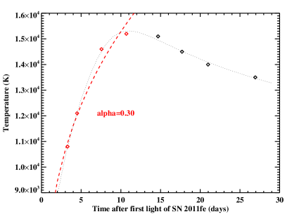
Figure 3.— Photospheric temperature fit for SN 2011fe. The dashed line presents a single power-law fit to the early-time data, while the dotted line represents a broken-power-law fit to all of the shown data.

One possible reason for this discrepancy could be changes in the temperature. When deriving Equation 2 from Equation 1, we assumed the temperature $T$ to be constant, which is unlikely to be true for SNe Ia. For SN 2011fe, Mazzali et al. (2014) found a significant increase in temperature during the first few days, a roughly constant temperature around peak brightness, and a relatively slow decay after peak. If we fit a power law to the first few days before peak (see Figure 3, dashed line), we find a rising index of $\alpha=0.30\pm 0.06$. This temperature increase would contribute together with $\alpha_{1v}$ to the final $\alpha_{r}$ value, which would be around $1.9=2\times(-0.20+1)+0.30$ (according to Equation 5), much closer to the observed value $\alpha_{r}\approx 2.1$.

Besides SN 2011fe, the temperature of SNe Ia does generally increase as a power law at early times. For example, Piro (2012) shows that the temperature could increase with a power-law index of 0.1 (see their Equation 30); though this is lower than what we found in SN 2011fe, the index depends on the parameters of individual SNe. Overall, the power-law increase in temperature could partially reduce the conflict between the different $\alpha_{1}$ values.

Even though we did not consider changes in temperature when deriving the function, the formulation of Equation 7 itself can in principle accommodate all contributions by adjusting the $\alpha_{r}$ value. This means that technically, it is fine to fit the light curves using Equation 7, but the relation in Equation 5 would not be valid owing to other contributions such as temperature changes. The parameter $\alpha_{r}$ could still represent the early-time rising index, though $\alpha_{1}$ would include not only the $\alpha_{1v}$ contribution but also the changes in temperature and perhaps other contributions. For example, we use the Si II $\lambda$6355 line to measure the photospheric velocity, but there is considerable debate regarding whether Si II $\lambda$6355 really does provide an accurate photospheric velocity (e.g., Blondin et al. et al. 2012). However, for our fitting purposes, it is reasonable to assume that there is a relation between the Si II $\lambda$6355 velocity and the photospheric velocity, even if the relation varies with time; Equation 7 can accommodate this through adjustments in the $\alpha_{r}$ value during the fitting process.

One may also notice that similar to $\alpha_{1}$, the $\alpha_{2}$ value from the light-curve fitting (around $-2.5$; see Table 1) differs from the photospheric velocity fitting ($\alpha_{2v}\approx 0$; see §3.1). The reason could be similar to that for $\alpha_{1}$; after peak brightness, the temperature decreases as the fireball expands, and the ejecta also become less dense. This causes the luminosity to drop fast, with a larger absolute value for the power-law index $\alpha_{2}$ (and $\alpha_{d}$). Technically, one can also fit the temperature with a broken power law (see Figure 3, dotted line); thus, both the increase and decrease of the power-law index would contribute to the light-curve fitting. But in order to simplify the fitting procedure, and considering that Equation 7 itself can accommodate the temperature changes by adjusting the $\alpha_{r}$ and $\alpha_{d}$ values, we did not explicitly include the temperature component in our model; however, its contribution has been included in $\alpha_{r}$ and $\alpha_{d}$ during the light-curve fitting.

Essentially, Equation 7 represents blackbody emission from the expanding fireball of a SN Ia. The radius of the fireball is proportional to the photospheric velocity, and therefore the equation is derived directly from the photospheric velocity evolution. Although when deriving Equation 7 we assumed the blackbody temperature is constant, the equation itself can accommodate the temperature changes – though the interpretation becomes more complicated if trying to distinguish the contributions from different components. Nevertheless, we see that the equation has a reasonable physical explanation, and it can be used to accurately fit SN Ia light curves during at least the first month after explosion.

3.4. Possible Application to Estimate $t_{0}$

In reality, very few SNe Ia other than SN 2011fe are discovered sufficiently early for their first-light time to be well estimated. However, a useful potential application from the above fitting method is that one can use Equation 7 to estimate the first-light or explosion time, $t_{0}$. For most SNe Ia, not discovered extremely early but instead around 1–2 weeks after first light and well monitored thereafter, by fitting the light curves using Equation 7 one can estimate $t_{0}$. This application will be presented by Zheng, Kelly & Filippenko (2017).

4. Conclusions

We have found a function with a reasonable physical explanation that can well fit SN Ia optical light curves. It is mathematically analytic and derived directly from the photospheric velocity evolution, adopting the simple assumption that the optical emission is approximately the blackbody emission of an expanding fireball. Applying this function to the case study of SN 2011fe gives surprisingly good results. Since SNe Ia share similar light-curve shapes, this fitting method has the potential to fit most other SNe Ia, providing valuable benefits for large datasets of SN Ia light curves obtained with current (e.g., Pan-STARRS; intermediate Palomar Transient Factory) and near-future (e.g., Zwicky Transient Facility; the Large Synoptic Survey Telescope) facilities.

References

- (1) Arnett, W. D. 1982, ApJ, 253, 785
- (2) Bazin, G., et al., 2011, A&A, 534, 43
- (3) Blondin, S., et al., 2012, ApJ, 2012
- (4) Cao, Y., et al. 2016, ApJ, 832, 86
- (5) Conley, A., et al., 2006, ApJ, 132, 1707
- (6) Firth, R. E., et al., 2015, MNRAS, 446, 3895
- (7) Ganeshalingam, M., Li, W., & Filippenko, A. V., 2011, MNRAS, 416, 2607
- (8) Guy, J., et al., 2007, A&A, 466, 11
- (9) Hachinger, S., et al., 2013, MNRAS, 429, 2228
- (10) Hayden B., et al., 2010, ApJ, 712, 350
- (11) Hillebrandt, W., & Niemeyer, J. C. 2000, ARA&A, 38, 191
- (12) Jha, S., et al., 2007, ApJ, 659, 122
- (13) Kim, A., et al., 2013, ApJ, 766, 84
- (14) Kessler, R., et al., 2010, PASP, 122, 1415
- (15) Li, W., et al. 2011, Nature, 480, 348
- (16) Mazzali, P. A., et al., 2014, MNRAS, 439, 1959
- Nugent et al. (2011) Nugent, P. E., et al. 2011, Nature, 480, 344
- (18) Piro, A., 2012, ApJ, 759, 83
- (19) Piro, A., & Nakar, E. 2013, ApJ, 769, 67
- (20) Piro, A., & Nakar, E. 2014, ApJ, 784, 85
- (21) Rabinak, I., Livne, E., & Waxman, E. 2012, ApJ, 757
- (22) Richmond, M. W., & Smith, H. A. 2012, JAVSO, 40, 872
- (23) Riess, A. G., et al. 1999, AJ, 118, 2675
- (24) Shappee, B., et al. 2016, ApJ, 826, 144
- Silverman et al. (2012) Silverman, J. M., et al. 2012, MNRAS, 425, 1819
- (26) Vinko, J., et al. 2012, A&A, 546, 12
- (27) Yamanaka, M., et al. 2009, ApJ, 707, L118
- (28) Zheng, W., Kelly, P. L., & Filippenko, A. V. 2017, submitted (arXiv:1612.02725)
- (29) Zheng, W., et al. 2012, ApJ, 751, 90
- (30) Zheng, W., et al. 2013, ApJ, 778, L15
- (31) Zheng, W., et al. 2014, ApJ, 783, L24
- (32) Zhang, K., et al. 2016, ApJ, 820, 67
- (33) Zheng, W., et al. 2017, submitted (arXiv:1611.09438)