High order ADER schemes for a unified first order hyperbolic formulation of Newtonian continuum mechanics coupled with electro-dynamics

Abstract

In this paper, we propose a new unified first order hyperbolic model of Newtonian continuum mechanics coupled with electro-dynamics. The model is able to describe the behavior of moving elasto-plastic dielectric solids as well as viscous and inviscid fluids in the presence of electro-magnetic fields. It is actually a very peculiar feature of the proposed PDE system that viscous fluids are treated just as a special case of elasto-plastic solids. This is achieved by introducing a strain relaxation mechanism in the evolution equations of the distortion matrix ${\bm{A}}$, which in the case of purely elastic solids maps the current configuration to the reference configuration. The model also contains a hyperbolic formulation of heat conduction as well as a dissipative source term in the evolution equations for the electric field given by Ohm's law. Via formal asymptotic analysis we show that in the stiff limit, the governing first order hyperbolic PDE system with relaxation source terms tends asymptotically to the well-known viscous and resistive magnetohydrodynamics (MHD) equations. Furthermore, a rigorous derivation of the model from variational principles is presented, together with the transformation of the Euler-Lagrange differential equations associated with the underlying variational problem from Lagrangian coordinates to Eulerian coordinates in a fixed laboratory frame. The present paper hence extends the unified first order hyperbolic model of Newtonian continuum mechanics recently proposed in [79, 28] to the more general case where the continuum is coupled with electro-magnetic fields. The governing PDE system is symmetric hyperbolic and satisfies the first and second principle of thermodynamics, hence it belongs to the so-called class of symmetric hyperbolic thermodynamically compatible systems (HTC), which have been studied for the first time by Godunov in 1961 [44] and later in a series of papers by Godunov and Romenski [49, 51, 84]. An important feature of the proposed model is that the propagation speeds of all physical processes, including dissipative processes, are finite. The model is discretized using high order accurate ADER discontinuous Galerkin (DG) finite element schemes with a posteriori subcell finite volume limiter and using high order ADER-WENO finite volume schemes. We show numerical test problems that explore a rather large parameter space of the model ranging from ideal MHD, viscous and resistive MHD over pure electro-dynamics to moving dielectric elastic solids in a magnetic field.

1 Introduction

In this paper, we propose a new unified first order hyperbolic model of Newtonian continuum mechanics coupled with electro-dynamics. The model is the extension of our previous results [28], hereafter Paper I, on a unified formulation of continuum mechanics towards the coupling of the time evolution equations for the matter with the electric and magnetic fields. The problem of determining the force acting on a medium in an electromagnetic field, as well as the related problem of determining the energy-momentum tensor of an electromagnetic field in a medium, has been discussed in the literature over the years since the work by Minkowski [67] and Abraham [1]. However, to the best of our knowledge, a universally accepted solution to this problem has been absent to date [62, 65, 42, 34, 23].

In this respect, our work can be broadly considered as a contribution to the modeling of electrodynamics of moving continuous media. We do not claim to give an ultimate solution to the problem, but rather to show that, within our formalism, all the equations can be obtained in a consistent way with rather good mathematical properties (symmetric hyperbolicity, first order PDEs, well posedeness of the initial value problem, finite speeds of perturbation propagation even for dissipative processes in the diffusive regime) and that the corresponding physical effects are correctly described. By an extensive comparison with the numerical and analytical solutions to the well established models as the Maxwell equations, ideal MHD equations and viscous resistive MHD (VRMHD) equations, we demonstrate that the proposed nonlinear hyperbolic dissipative model is able to describe dielectrics ($\eta\rightarrow\infty$), ideal conductors ($\eta\rightarrow 0$), and resistive conductors ($0<\eta<\infty$) as particular cases, where $\eta$ is the resistivity. Thus, the applicability range of the proposed model is larger than those for ideal and resistive MHD models, because the electric and magnetic fields are genuinely independent and are governed by their own time evolution equations as in the Maxwell equations.

In Paper I and [79], we provided a unified first-order hyperbolic formulation of the equations of continuum mechanics, showing for the first time that the dynamics of fluids and solids can be cast in a single mathematical framework. This becomes possible due to the use of a characteristic strain dissipation time $\tau$, which is the characteristic time for continuum particle rearrangements. By its definition, the characteristic time $\tau$, as opposed to the viscosity coefficient, is applicable to the dynamics of both fluids and solids (see the discussions in [79] and Paper I) and is a continuum interpretation of the seminal idea of the so-called particle settled life time (PSI) of Frenkel [37], who applied it to describe the fluidity of liquids, see also [14, 12, 13] and references therein. In addition, the definition of $\tau$ assumes the continuum particles to have a finite scale and thus to be deformable as opposed to the scaleless mathematical points in classical continuum mechanics. We note that the model studied in [79] and Paper I was used by several authors, e.g. [83, 66, 81, 39, 9, 48, 36, 82, 8, 71, 78] to cite just a few, in the solid dynamics context since its original invention in 1970th by Godunov and Romenski [50, 46] but the recognition that the same model is also applicable to the dynamics of viscous fluids and its extensive validation in the fluid dynamics context was made only recently in [79] and Paper I.

What concerns a mathematical guide to derive time evolution equations, as in [79] and Paper I, we follow the so-called formalism of Hyperbolic Thermodynamically Compatible systems of conservation laws, or simply HTC formalism here. This formalism is described in Section 2. We recall that hyperbolicity naturally accounts for the two most relevant features of fundamental physical systems, namely the unique and continuous dependence of the solution on the initial data, and the finite velocity for perturbation propagation (causality).

At this point we stress that the HTC theory is radically different from classical Maxwell-Cattaneo hyperbolic relaxation models [16, 59, 70] typically used in extended irreversible thermodynamics (EIT), since the propagation speeds of all physical processes remain finite, even in the stiff relaxation limit (parabolic diffusion limit), see [79] for a more detailed discussion. The differences between the approaches become also apparent if one takes a look at the physical meaning of the state variables used in both approaches. We recall that in the EIT the fluxes are typically used as the extra state variables (in addition to the conventional ones like mass, momentum and energy), which usually leads to the result that the PDEs have no apparent structure. In the HTC formalism, only density fields may serve as state variables which, in fact, due to the fundamental conservation principle allows to obtain equations in a rather complete form with an elegant structure, see Section 2.

For recent work on hyperbolic reformulations of the steady viscous and resistive MHD equations and time dependent convection-diffusion equations based on standard Maxwell-Cattaneo relaxation, see the papers of Nishikawa et al. [72, 73, 10] and Montecinos and Toro [69, 68, 90].

The plan of the paper is the following: in the first part we concentrate on the mathematical principles of the HTC system (Sections 2 and 3), while in the second part we give an extensive numerical evidences of the applicability of the model to a wide range of electromagnetic flows.

In the rest of the paper we use the Einstein summation convention over repeated indices.

2 HTC formalism and the master system

The hyperbolic dissipative theory discussed in this paper relies on the HTC formalism. The development of the formalism started in 1961 after it was observed by Godunov [44, 43] that some systems of conservation laws admitting an extra conservation law also admit an interesting parametrization

$$\dfrac{\mathcal{\partial}M_{p_{i}}}{\mathcal{\partial}t}+\dfrac{\mathcal{\partial}N^{j}_{p_{i}}}{\mathcal{\partial}y_{j}}=0$$ (1)

which allows to rewrite the governing equations in a symmetric form

$$M_{p_{i}p_{k}}\dfrac{\mathcal{\partial}p_{k}}{\mathcal{\partial}t}+N^{j}_{p_{i}p_{k}}\dfrac{\mathcal{\partial}p_{k}}{\mathcal{\partial}y_{j}}=0.$$ (2)

Here, $t$ is the time, $y_{j}$ are the spatial coordinates, $p_{k}$ is the vector of state variables, $M(p_{i})$ and $N^{j}(p_{i})$ are the scalar potentials of the state variables. Here and in the rest of the paper, a potential with the state variables in the subscript should be understood as the partial derivatives of the potential with respect to these state variables. Thus, for example, $M_{p_{k}}$, $N^{j}_{p_{k}}$, $M_{p_{i}p_{k}}$ and $N^{j}_{p_{i}p_{k}}$ in (1)–(2) should be understood as the first and second partial derivatives of the potentials $M$ and $N^{j}$ with respect to the state variables $p_{i}$, e.g. $M_{p_{k}}=\mathcal{\partial}M/\mathcal{\partial}p_{k}$, $M_{p_{i}p_{k}}=\mathcal{\partial}^{2}M/\mathcal{\partial}p_{i}\mathcal{\partial}p_{k}$, etc.

In this parametrization, the extra conservation law has always the following form

$$\dfrac{\mathcal{\partial}(p_{i}M_{p_{i}}-M)}{\mathcal{\partial}t}+\dfrac{\mathcal{\partial}(p_{i}N^{j}_{p_{i}}-N^{j})}{\mathcal{\partial}y_{j}}=0$$ (3)

and, in fact, it is just a straightforward consequence of the governing equations (1) and can be obtained as a linear combination of these equations. Indeed, (3) can be obtained as a sum of the equations (1) multiplied by the corresponding factors $p_{i}$.

If the potential $M(p_{i})$ is a strictly convex function of the state variables then the symmetric matrix $M_{p_{i}p_{k}}$ is positive definite and (2) becomes a symmetric hyperbolic system of equations [38].

Usually, the generating potential $M$ has the meaning of the generalized pressure while its Legendre transformation $p_{i}M_{p_{i}}-M$ has the meaning of the total energy and thus, (3) is the total energy conservation law. Hence, the observation of Godunov establishes the very important connection between the well-posedeness of the equations of mathematical physics and thermodynamics.

As it was understood later on the examples of the ideal MHD equations [45], that the original observation of Godunov [44] relates only to conservation laws written in the Lagrangian frame which indeed admits a fully conservative formulation, while the time evolution equations in the Eulerian frame have a more complicated structure, except for the compressible Euler equations of ideal fluids.

The structure of the Eulerian equations and its relation to the fully conservative structure of the equations in Lagrangian form was revealed in a series of papers by Godunov and Romenski [51, 52, 47, 53, 84, 85, 54]. In particular, in [47], based on the group representation theory [41], a rather general form of first order PDEs with the following properties was proposed:

• PDEs are invariant under rotations

• PDEs are compatible with an extra conservation law

• PDEs are generated by only one potential like $M$

• PDEs are symmetric hyperbolic

• PDEs are conservative and generated by invariant differential operators only, such as div, grad and curl.

One may naturally question how this class of PDEs, which shall be referred to as as the master system, relates to the models that describe continuum mechanics and whether it is too restrictive to deal with dissipative processes such as viscous momentum transfer, heat transfer, resistive MHD, etc., typically described by second order parabolic equations. First, it is important to emphasize that invariance under orthogonal transformations and the existence of an extra conservation law, which is typically the total energy conservation, is the compulsory requirement for continuum mechanics models. Second, as shown recently [79, 28], there is no physical reason imposing that the dissipative transport processes such as viscous momentum transfer or heat conduction should be exclusively modeled by the second order parabolic diffusion theory, but they can also be very successfully modeled by a more general framework based on first order hyperbolic equations with relaxation source terms. Third, after analysis of a rather large number of particular examples of continuum models [51, 52, 53, 84, 85], it was shown that many models fall into the class of HTC systems. Among them are the compressible Euler equations of ideal fluids, the ideal MHD equations, the equations of nonlinear elasto-plasticity, the electrodynamics of moving media, a model describing superfluid helium, the equations governing compressible multi-phase flows, elastic superconductors, and finally also the unified first order hyperbolic formulation for fluid and solid mechanics introduced in [79, 28]. In this paper, we show that also the viscous and resistive MHD equations can be cast into the form of a first order HTC system.

The starting point of the HTC formalism is a sub-system of the Lagrangian conservation laws given in eqs. (1) of  [47], which will be refereed to as the master system from now on. The final governing PDEs written in the Eulerian frame will then be the result of the following system of Lagrangian master equations:

$$\displaystyle\frac{{\rm d}M_{v_{i}}}{{\rm d}t}-\frac{\partial P_{ij}}{\partial y_{j}}=0,$$ (4a)

$$\displaystyle\frac{{\rm d}M_{P_{ij}}}{{\rm d}t}-\frac{\partial v_{i}}{\partial y_{j}}=0,$$ (4b)

$$\displaystyle\frac{{\rm d}M_{d_{i}}}{{\rm d}t}-\varepsilon_{ijk}\frac{\partial b_{k}}{\partial y_{j}}=0,$$ (4c)

$$\displaystyle\frac{{\rm d}M_{b_{i}}}{{\rm d}t}+\varepsilon_{ijk}\frac{\partial d_{k}}{\partial y_{j}}=0.$$ (4d)

Here, $v_{i}$ is the velocity of the matter, $P_{ij}$ is the stress tensor, while $d_{i}$ and $b_{i}$ are some vectors describing the electric and magnetic fields, respectively.

In contrast to the classical parabolic theory of dissipative processes, the governing equations in our approach are all first order hyperbolic PDEs and the dissipative processes will not be modeled by differential terms, but exclusively via algebraic relaxation source terms, which will be specified later in the Eulerian case. This has the important consequence that the structure of the differential terms and the type of the PDE is the same in both, the dissipative as well as in the non-dissipative case. We recall, that if the dissipation is excluded in the classical second order parabolic diffusion theory, this then changes not only the structure of the PDEs, but also their type.

Because of this fact, within the HTC formalism we can study the structure of the governing equations by restricting our considerations to the non-dissipative case only. We also note that if the dissipation source terms are switched off, then the model describes an elastic medium, see [79, 28].

2.1 Variational nature of the field equations in a moving elastic medium

It is well known that many equations of mathematical physics can be derived as the Euler-Lagrange equations obtained by the minimization of a Lagrangian. As an example, one can consider the nonlinear elasticity equations in Lagrangian coordinates [55]. The classical Maxwell equations of electrodynamics can also be derived by the minimization of a Lagrangian with the use of the gauge theory [40]. It turns out that the coupling of these two physical objects in a single Lagrangian gives us a straightforward way to derive the equations for the electromagnetic field in a moving medium. We start by introducing two vector potentials and a scalar potential:

$${\bm{x}}=[x_{i}(t,{\bm{y}})],\ \ \ {\bm{a}}=[a_{i}(t,{\bm{y}})],\ \ \ \varphi(t,{\bm{y}}),$$ (5)

so that

$$\hat{v}_{i}=\dfrac{\mathcal{\partial}x_{i}}{\mathcal{\partial}t},\ \ \ \hat{F}_{ij}=\dfrac{\mathcal{\partial}x_{i}}{\mathcal{\partial}y_{j}},$$ (6)

$$\hat{e}_{i}=-\dfrac{\mathcal{\partial}a_{i}}{\mathcal{\partial}t}-\dfrac{\mathcal{\partial}\varphi}{\mathcal{\partial}y_{i}},\ \ \ \hat{h}_{i}=\varepsilon_{ijk}\dfrac{\mathcal{\partial}a_{k}}{\mathcal{\partial}y_{j}},$$ (7)

Here, $t$ is time, ${\bm{y}}=[y_{i}]$ and ${\bm{x}}=[x_{i}]$ are the Lagrangian and Eulerian spatial coordinates respectively, while ${\bm{a}}$ and $\varphi$ are the conventional electromagnetic potentials.

Then, we define the action integral

$${\mathcal{L}}=\int\Lambda d{\bm{y}}dt,$$ (8)

where $\Lambda=\Lambda(\hat{v}_{i},\hat{F}_{ij},\hat{e}_{i},\hat{h}_{i},\hat{w}_{i},\hat{c})$ is the Lagrangian.

First variation of $\mathcal{L}$ gives us the Euler-Lagrange equations

$$\dfrac{\partial\Lambda_{\hat{v}_{i}}}{\partial t}+\dfrac{\partial\Lambda_{\hat{F}_{ij}}}{\partial y_{j}}= \ \ 0,$$ (9)

$$\dfrac{\partial\Lambda_{\hat{e}_{i}}}{\partial t}+\varepsilon_{ijk}\dfrac{\partial\Lambda_{\hat{h}_{k}}}{\partial y_{j}}= \ \ 0,$$ (10)

$$\dfrac{\mathcal{\partial}\Lambda_{\hat{e}_{j}}}{\mathcal{\partial}y_{j}}= \ \ 0.$$ (11)

To this system, the following compatibility constraints should be added (they are trivial consequences of the definitions (6) and (7))

$$\frac{\mathcal{\partial}\hat{F}_{ij}}{\mathcal{\partial}t}-\frac{\mathcal{\partial}\hat{v}_{i}}{\mathcal{\partial}y_{j}} =0\,, \dfrac{\partial\hat{F}_{ij}}{\partial y_{k}}-\dfrac{\partial\hat{F}_{ik}}{\partial y_{j}}=0\,,$$ (12)

$$\frac{\mathcal{\partial}\hat{h}_{i}}{\mathcal{\partial}t}+\varepsilon_{ijk}\dfrac{\mathcal{\partial}\hat{e}_{k}}{\mathcal{\partial}y_{j}} =0\,, \dfrac{\partial\hat{h}_{j}}{\partial y_{j}}=0\,.$$ (13)

In order to rewrite equations (9)–(13) in the form of system (4), let us introduce the potential $U$ as a partial Legendre transformation of the Lagrangian $\Lambda$

$${\rm d}U = {\rm d}(\hat{v}_{i}\Lambda_{\hat{v}_{i}}+\hat{e}_{i}\Lambda_{\hat{e}_{i}}-\Lambda)=\hat{v}_{i}{\rm d}\Lambda_{\hat{v}_{i}}+\hat{e}_{i}{\rm d}\Lambda_{\hat{e}_{i}}-\Lambda_{\hat{F}_{ij}}{\rm d}\hat{F}_{ij}-\Lambda_{\hat{h}_{i}}{\rm d}\hat{h}_{i}=$$ (14)

$$\hat{v}_{i}{\rm d}\Lambda_{\hat{v}_{i}}+\hat{e}_{i}{\rm d}\Lambda_{\hat{e}_{i}}+\Lambda_{\hat{F}_{ij}}{\rm d}(-\hat{F}_{ij})+\Lambda_{\hat{h}_{i}}{\rm d}(-\hat{h}_{i}).$$

Hence, denoting $m_{i}=\Lambda_{\hat{v}_{i}}$, $e_{i}=\Lambda_{\hat{e}_{i}}$, $F_{ij}=-\hat{F}_{ij}$, $h_{i}=-\hat{h}_{i}$, we get the thermodynamic identity

$${\rm d}U=U_{m_{i}}{\rm d}m_{i}+U_{F_{ij}}{\rm d}F_{ij}+U_{e_{i}}{\rm d}e_{i}+U_{h_{i}}{\rm d}h_{i}.$$

Eventually, in terms of the variables

$${\mathbf{q}}=(m_{i},F_{ij},e_{i},h_{i})$$ (15)

and the potential $U=U({\mathbf{q}})$, equations (9), (10), (12)₁ and (13)₁ become

$$\displaystyle\frac{{\rm d}m_{i}}{{\rm d}t}-\frac{\partial U_{F_{ij}}}{\partial y_{j}}=0,$$ (16a)

$$\displaystyle\frac{{\rm d}F_{ij}}{{\rm d}t}-\frac{\partial U_{m_{i}}}{\partial y_{j}}=0,$$ (16b)

$$\displaystyle\frac{{\rm d}e_{i}}{{\rm d}t}-\varepsilon_{ijk}\frac{\partial{U}_{h_{k}}}{\partial y_{j}}=0,$$ (16c)

$$\displaystyle\frac{{\rm d}h_{i}}{{\rm d}t}+\varepsilon_{ijk}\frac{\partial{U}_{e_{k}}}{\partial y_{j}}=0\,,$$ (16d)

which should be supplemented by stationary constraints (11), (12)₂ and (13)₂ which now read as

$$\dfrac{\partial F_{ij}}{\partial y_{k}}-\dfrac{\partial F_{ik}}{\partial y_{j}}=0\,,\qquad\dfrac{\mathcal{\partial}e_{i}}{\mathcal{\partial}y_{i}}=0\,,\qquad\dfrac{\mathcal{\partial}h_{i}}{\mathcal{\partial}y_{i}}=0\,.$$ (17)

System (16) is, in fact, identical to (4). In order to see this, one needs to introduce fluxes as new (conjugate) state variables

$${\mathbf{p}}=(U_{m_{i}},U_{F_{ij}},U_{e_{i}},U_{h_{i}}),$$ (18)

which we denote as

$$\begin{array}[]{cc}v_{i}=U_{m_{i}},&P_{ij}=U_{F_{ij}},\\[5.69054pt] d_{i}=U_{e_{i}},&b_{i}=U_{h_{i}},\end{array}$$ (19)

and a new potential $M({\mathbf{p}})$ as a Legendre transform of $U({\mathbf{q}})$, i.e.

$$M=m_{i}U_{m_{i}}+F_{ij}U_{F_{ij}}+e_{i}U_{e_{i}}+h_{i}U_{h_{i}}-U,$$ (20)

or briefly

$$M({\mathbf{p}})={\mathbf{q}}\cdot{\mathbf{p}}-U({\mathbf{q}}).$$ (21)

After that, system (16) transforms exactly to (4), while constraints (17) read as

$$\dfrac{\partial M_{P_{ij}}}{\partial y_{k}}-\dfrac{\partial M_{P_{ik}}}{\partial y_{j}}=0\,,\qquad\dfrac{\mathcal{\partial}M_{d_{i}}}{\mathcal{\partial}y_{i}}=0\,,\qquad\dfrac{\mathcal{\partial}M_{b_{i}}}{\mathcal{\partial}y_{i}}=0\,.$$ (22)

One may clearly note, a similarity between the equations (4c)–(4d) (or (16c)–(16d)) and the Maxwell equations. However, because no assumptions about the Lagrangian $\Lambda$, and thus, about the potentials $U({\mathbf{q}})$ and $M({\mathbf{p}})$, has been done yet, these equations should be considered as a nonlinear generalization of the Maxwell equations.

We note that equations (4a)–(4b) and (4c)–(4d) (or (16a)–(16b) and (16c)–(16d)) are not independent as it may seem. They are coupled via the dependence of the potential $M({\mathbf{p}})$ (or $U({\mathbf{q}})$) on all the state variables (15). This coupling will emerge in a more transparent way when we shall consider these equations in the Eulerian frame in Section 3.

2.2 Properties of the master system

2.2.1 Energy conservation

A central role in the system formulation is played by the thermodynamic potential

$$U=U(m_{i},F_{ij},e_{i},h_{i}).$$ (23)

or its dual

$$M=M(v_{i},P_{ij},d_{i},b_{i})$$ (24)

as one of them generates the fluxes in (16), while the other generates the density fields in (4). The potential $U$ typically has the meaning of the total energy density of the system, while $M$ has the meaning of a total pressure.

In addition, solutions of the system (16) satisfy an extra conservation law

$$\frac{{\rm d}{U}}{{\rm d}t}-\frac{\partial}{\partial y_{j}}\left(U_{m_{i}}U_{F_{ij}}+\varepsilon_{ijk}U_{e_{i}}{U}_{h_{k}}\right)=0$$ (25)

which should be interpreted as the total energy conservation. In terms of the dual potential $M$ and dual state variables (19) it reads as

$$\frac{{\rm d}}{{\rm d}t}\left(v_{i}M_{v_{i}}+P_{ij}M_{P_{ij}}+d_{i}M_{d_{i}}+b_{i}M_{b_{i}}-M\right)-\frac{\partial}{\partial y_{j}}\left(v_{i}P_{ij}+\varepsilon_{ijk}d_{i}{b}_{k}\right)=0.$$ (26)

The energy conservation law (25) is not independent but a consequence of all the equations (16). Indeed, if we multiply each equation in (16) by a corresponding factor and sum up the result, we obtain equation (25) identically:

$$U_{m_{i}}\cdot(\ref{eqn.MasterLagr.Momentum})+U_{F_{ij}}\cdot(\ref{eqn.MasterLagr.F})+U_{e_{i}}\cdot(\ref{eqn.MasterLagr.Electr})+U_{h_{i}}\cdot(\ref{eqn.MasterLagr.Magn})\equiv(\ref{eqn.EnergyConsLagr}).$$ (27)

The same is true for (26) and (4).

2.2.2 Possible interpretation of the state variables

Usually, the derivation of a model begins with the choice of state variables. In the context of classical hydrodynamics, the answer is universal. The state variables are the classical hydrodynamic fields such as mass, momentum, entropy, or total energy. In any case which is beyond the inviscid hydrodynamics settings, the choice of extra state variables is not universal. In the HTC formalism, we however follow a different strategy, which consists of two stages. In the first stage, the governing equations are formulated before any choice of extra state variables has been made. The structure of the governing PDEs is a consequence of the five fundamental requirements formulated earlier in this Section. The physical meaning of the state variables becomes clear at the second stage, when we try to compare a solution to the model with specific experimental observations. At this stage, we simultaneously clarify the meaning of the state variables and look for an appropriate energy potential which can be seen also as the choice of the constitutive relations in the classical continuum mechanics. For the proposed model, this strategy is realized in Section 3.3.

Thus, in this Section, we give only approximate interpretations of the state variables while their precise meanings will be given in Section 3.3. As stated above, the space variables ${\bm{y}}=[y_{i}]$ can be treated as the Lagrangian coordinates which are connected to the Eulerian coordinates ${\bm{x}}(t)=[x_{i}(t)]$ measured relative to a laboratory frame by the equality $y_{i}=x_{i}(0)$. It is also implied that $v_{i}=\frac{{\rm d}x_{i}}{{\rm d}t}$ in (4) is the velocity of the matter relative to the laboratory frame, while $m_{i}=M_{v_{i}}$ in (16) has a meaning of a generalized momentum density which may include contributions from other physical processes and in general depends on the specification of the potential $M$, or $U$. As it will be shown in Section 3.3, $m_{i}$ couples the material momentum and electromagnetic momentum (Poynting vector). The tensorial variable $F_{ij}=\frac{\partial x_{i}}{\partial y_{j}}$ is the deformation gradient, $e_{i}$ and $h_{i}$ are the electric and magnetic fields, respectively. However, the exact meaning of the fields $e_{i}$ and $h_{i}$ will be clarified later in Section 3 when we shall distinguish among different reference frames.

2.2.3 Symmetric hyperbolicity

System (4) can be rewritten in a symmetric quasilinear from

$$\mathbb{M}\frac{\mathcal{\partial}{\mathbf{p}}}{\mathcal{\partial}t}+\mathbb{N}_{j}\frac{\mathcal{\partial}{\mathbf{p}}}{\mathcal{\partial}y_{j}}=0,$$ (28)

with the symmetric matrix $\mathbb{M}({\mathbf{p}})=M_{{\mathbf{p}}{\mathbf{p}}}=[\mathcal{\partial}^{2}M/\mathcal{\partial}p_{i}\mathcal{\partial}p_{j}]$ and constant symmetric matrices $\mathbb{N}_{j}$ consisting only of $1$, $-1$ and zeros. Moreover, system (4) is symmetric hyperbolic if $M({\mathbf{p}})$ is convex. In other words, the Cauchy problem for (4) (as well as for (16)) is automatically well posed locally in time for smooth initial data [18]. We recall that the convexity of $M({\mathbf{p}})$ is equivalent to the convexity of $U({\mathbf{q}})$ due to the properties of the Legendre transformation.

2.2.4 ${\mathbf{q}}$ and ${\mathbf{p}}$-type state variables

We emphasize the very distinct nature of the variables ${\mathbf{q}}$ and ${\mathbf{p}}$. Namely, the variables ${\mathbf{q}}$ appear in the time derivative and have the meaning of densities (volume average quantities), we thus shall refer to components of ${\mathbf{q}}$ as density fields. On the other hand, the variables ${\mathbf{p}}$ appear as fluxes in the master system (16) (or (4)), and thus will be referred to as flux fields (surface defined quantities). See also discussion in [78]. In the HTC formalism, the potential $M({\mathbf{p}})$ (the generalized pressure) and the flux fields ${\mathbf{p}}$ are conjugate quantities to the potential $U({\mathbf{q}})$ (total energy density) and the density fields ${\mathbf{q}}$, i.e. there are connected by the following identities

$$p_{i}=U_{q_{i}},\qquad q_{i}=M_{p_{i}}$$ (29)

and

$$M=q_{i}U_{q_{i}}-U,\qquad U=p_{i}M_{p_{i}}-M.$$ (30)

Thus, it follows from (29) that, in order the nonlinear change of variables (29) be a one-to-one map, one should require that the potentials $U({\mathbf{q}})$ and $M({\mathbf{p}})$ be convex functions because

$$M_{{\mathbf{p}}{\mathbf{p}}}=\frac{\mathcal{\partial}{\mathbf{q}}}{\mathcal{\partial}{\mathbf{p}}}=\left[\frac{\mathcal{\partial}{\mathbf{p}}}{\mathcal{\partial}{\mathbf{q}}}\right]^{-1}=U_{{\mathbf{q}}{\mathbf{q}}}.$$ (31)

2.2.5 Stationary constraints

Solutions to system (16) satisfy some stationary conservation laws that are compatible with system (16) and conditioned by the structure of the flux terms:

$$\dfrac{\partial F_{ij}}{\partial y_{k}}-\dfrac{\partial F_{ik}}{\partial y_{j}}=0,\ \ \ \dfrac{\partial e_{k}}{\partial y_{k}}=0,\ \ \ \dfrac{\partial h_{k}}{\partial y_{k}}=0.$$ (32)

These stationary laws hold for every $t>0$ if they are valid at $t=0$, and thus should be considered as the constraints on the initial data. Indeed, applying the divergence operator, for instance, to equations (16d) we obtain

$$\dfrac{\partial}{\partial t}\left(\dfrac{\partial h_{k}}{\partial y_{k}}\right)=0,$$ (33)

which yields the third equation in (32) if it was fulfilled at the initial time. The other laws can be obtained in a similar way. As we shall discuss later on the example of the Eulerian equations, the situation is rather different in the Eulerian setting, and the stationary constraints like (32) are not separate but an intrinsic part of the structure of the governing equations written in the Eulerian frame.

2.2.6 Complimentary structure

We also note a complimentary structure of equations (16) and (4), i.e. the PDEs are split into pairs. In each pair, a variable appearing in the time derivative, say $u_{i}$ in (16a), then appears in the flux of the complimentary equation as $U_{u_{i}}$ in (16b). Thus, $u_{i}$ and $F_{ij}$ are complimentary variables, as well as $e_{i}$ and $h_{i}$. This means, that a physical process should be always presented at least by two state variables and hence by two PDEs in the HTC formalism. One may note a close relation of such a complimentary structure of the HTC formalism and the odd and even parity of the state variables with respect to the time-reversal transformation in the context of the GENERIC (general equation of nonequilibrium reversible-irreversible coupling) formalism discussed in [77].

3 Master system in the Eulerian frame

In this section, we formulate a system of governing equations describing motion of a heat conducting deformable medium (fluid or solid) in the electromagnetic field in the Eulerian frame. This system is obtained as a direct consequence of the master system (16) by means of the Lagrange-to-Euler change of variables: ${\bm{y}}\rightarrow{\bm{x}}$. This transformation is a nontrivial task, and the details are given in B for the electromagnetic field equations and in C for the momentum conservation law while the details about the derivation of the other equations can be found in the Appendix in [78] or in [47]. We give the Eulerian formulations using both density fields ${\mathbf{q}}$ and flux fields ${\mathbf{p}}$. As we shall see, the Eulerian equations do not have such a simple structure as the Lagrangian equations. Nevertheless, we stress that none of the differential terms was prescribed ``by hand'', but all of them are a direct consequence of the ${\bm{y}}\rightarrow{\bm{x}}$ variable transformation solely.

3.1 $({\mathcal{E}},{\mathbf{q}})$-formulation

The main system of governing equations studied in this paper is formulated in terms of ${\mathbf{q}}$-type state variables (density fields, see Section 2.2.4)

$${\mathbf{q}}=(\rho,\mathbf{m},{\bm{A}},{\mathbf{e}},{\mathbf{h}},\mathbf{w},\sigma),$$ (34)

and the total energy density $\mathcal{E}(\mathbf{q})=w^{-1}U$, where $U$ is the Lagrangian total energy density introduced in Section 2, $\rho$ is the mass density, $\sigma=\rho s$ is the entropy density, $s$ is the specific entropy, $\mathbf{m}=[m_{i}]$ is a generalized momentum density which couples the ordinary matter momentum density, $\rho{\mathbf{v}}$, with the electromagnetic momentum density, i.e. the Poynting vector. The exact expression for $\mathbf{m}$ will be given later. Matrix ${\bm{A}}=[A_{ik}]$ is the distortion field (see Paper I), ${\mathbf{e}}=[e_{i}]$ and ${\mathbf{h}}=[h_{i}]$ are the vector fields which relate to the electro-magnetic fields and will be specified later, $\mathbf{w}=\rho{\mathbf{J}}$ is the thermal impulse density (see Paper I), which can be interpreted as an average momentum density of the heat carriers. The velocity of the media, ${\mathbf{v}}$, is not a primary state variable and should be computed from the generalized momentum $\mathbf{m}$, but also, according to the HTC formalism, the velocity and the generalized momentum relate to each other as $v_{i}={\mathcal{E}}_{m_{i}}$ (see (19) and the discussion below). In the Eulerian coordinates $x_{k}$, the system of governing equations reads as

$$\frac{\partial\rho}{\partial t}+\frac{\partial(\rho v_{k})}{\partial x_{k}}=0,$$ (35a)

$$\displaystyle\frac{\partial m_{i}}{\partial t}+\frac{\partial}{\partial x_{k}}\left(m_{i}v_{k}+\delta_{ik}\left(\rho{\mathcal{E}}_{\rho}+m_{l}{\mathcal{E}}_{m_{l}}+e_{l}{\mathcal{E}}_{e_{l}}+h_{l}{\mathcal{E}}_{h_{l}}-{\mathcal{E}}\right)+A_{li}{\mathcal{E}}_{A_{lk}}-e_{k}{\mathcal{E}}_{e_{i}}-h_{k}{\mathcal{E}}_{h_{i}}\right)=0,$$ (35b)

$$\displaystyle\frac{\partial A_{ik}}{\partial t}+\frac{\partial(A_{il}v_{l})}{\partial x_{k}}+v_{j}\left(\frac{\partial A_{ik}}{\partial x_{j}}-\frac{\partial A_{ij}}{\partial x_{k}}\right)=-\dfrac{{\mathcal{E}}_{A_{ik}}}{\rho\,\theta_{1}(\tau_{1})},$$ (35c)

$$\displaystyle\frac{\partial e_{i}}{\partial t}+\frac{\partial\left(e_{i}v_{k}-v_{i}e_{k}-\varepsilon_{ikl}{\mathcal{E}}_{h_{l}}\right)}{\partial x_{k}}+v_{i}\dfrac{\mathcal{\partial}e_{k}}{\mathcal{\partial}x_{k}}=-\frac{{\mathcal{E}}_{e_{i}}}{\eta},$$ (35d)

$$\displaystyle\frac{\partial h_{i}}{\partial t}+\frac{\partial\left(h_{i}v_{k}-v_{i}h_{k}+\varepsilon_{ikl}{\mathcal{E}}_{e_{l}}\right)}{\partial x_{k}}+v_{i}\dfrac{\mathcal{\partial}h_{k}}{\mathcal{\partial}x_{k}}=0,$$ (35e)

$$\displaystyle\frac{\partial w_{i}}{\partial t}+\frac{\partial\left(w_{i}v_{k}+{\mathcal{E}}_{\sigma}\delta_{ik}\right)}{\partial x_{k}}=-\dfrac{\rho\,{\mathcal{E}}_{w_{i}}}{\theta_{2}(\tau_{2})},$$ (35f)

$$\displaystyle\frac{\partial\sigma}{\partial t}+\frac{\partial\left(\sigma v_{k}+{\mathcal{E}}_{w_{k}}\right)}{\partial x_{k}}=\frac{1}{{\mathcal{E}}_{\sigma}}\left(\dfrac{1}{\rho\theta_{1}}{\mathcal{E}}_{A_{ik}}{\mathcal{E}}_{A_{ik}}+\dfrac{\rho}{\theta_{2}}{\mathcal{E}}_{w_{i}}{\mathcal{E}}_{w_{i}}+\frac{1}{\eta}{\mathcal{E}}_{e_{i}}{\mathcal{E}}_{e_{i}}\right)\geq 0.$$ (35g)

The energy conservation law

$$\frac{\partial{\mathcal{E}}}{\partial t}+\frac{\partial}{\partial x_{k}}\left(v_{k}{\mathcal{E}}+v_{i}\left[\left(\rho{\mathcal{E}}_{\rho}+m_{l}{\mathcal{E}}_{m_{l}}+e_{l}{\mathcal{E}}_{e_{l}}+h_{l}{\mathcal{E}}_{h_{l}}-{\mathcal{E}}\right)\delta_{ik}+A_{li}{\mathcal{E}}_{A_{lk}}-e_{k}{\mathcal{E}}_{e_{i}}-h_{k}{\mathcal{E}}_{h_{i}}\right]\phantom{1^{1}}\right.\\ \left.+\varepsilon_{ijk}{\mathcal{E}}_{e_{i}}{\mathcal{E}}_{h_{j}}+{\mathcal{E}}_{\sigma}{\mathcal{E}}_{w_{k}}\right)=0$$ (36)

is a consequence of equations (35), i.e. it can be obtained by means of the summation rule (27). We emphasize that in the numerical computations shown later in Section 4, we solve the energy equation (36) instead of the entropy equation (35g), but from the point of view of the model formulation, the entropy should be considered among the vector of unknowns because it is the complementary variable to the thermal impulse $\mathbf{w}=\rho{\mathbf{J}}$, see the remark in Section 2.2.6 and Paper I.

All equations in system (35) except the continuity equation (35a) and the heat conduction equation (35f)–(35g) originate from the Lagrangian equations with the structure (16). The momentum equation and the distortion equation are derived from the pair (16a)–(16b), the electromagnetic field equations (35d)–(35e) are derived from the pair (16c)–(16d).

The energy conservation law (36) is the consequence of equations (35), since it can be obtained as a linear combination of all equations (35) with coefficients introduced in the following section. As in the Lagrangian frame, these coefficients (multipliers) are the thermodynamically conjugate state variables and have the meaning of fluxes.

As discussed in [79, 28], the distortion field ${\bm{A}}$ describes deformability and orientation of the continuum particles which assume to have a finite (non-zero) length scale. Macroscopic flow is naturally considered as the process of continuum particles rearrangements in the HTC model. Because of the rearrangements of particles, the field ${\bm{A}}$ is not integrable in the sense that it does not relate Eulerian and Lagrangian coordinates of the continuum. As a result, the field ${\bm{A}}$ is local and it relates to the deformation gradient ${\bm{F}}$ introduced in Section 2.1 only via

$$\det({\bm{F}})=1/\det({\bm{A}}).$$ (37)

However, if we consider a particular case of system (35) when the dissipation term in the right hand side of (35c) is absent, which corresponds to an elastic solid (e.g. see the last numerical example in Paper I), then we have that ${\bm{A}}={\bm{F}}^{-1}$.

For simplicity, we use the same notations $m_{i}$, $e_{i}$ and $h_{i}$ for the generalized momentum, electric and magnetic fields in both the Lagrangian and the Eulerian framework. However, these fields are different, see B. For example, if we denote by $\mathbf{m}_{L}$, ${\mathbf{e}}_{L}$ and ${\mathbf{h}}_{L}$ the Lagrangian fields, i.e. exactly those fields which are used in equations (16a), (16c) and (16d), then they are related to $\mathbf{m}$, ${\mathbf{e}}$ and ${\mathbf{h}}$ appearing in the Eulerian equations (35b), (35d) and (35e) as

$$\mathbf{m}_{L}=w\,\mathbf{m},\ \ \ {\mathbf{e}}_{L}=w{\bm{F}}^{-1}{\mathbf{e}},\ \ \ {\mathbf{h}}_{L}=w{\bm{F}}^{-1}{\mathbf{h}},$$ (38)

where $w=\det({\bm{F}})=1/\det({\bm{A}})$, and ${\bm{F}}$ is the deformation gradient introduced in Section 2.1. Subsequently, the Lagrangian total energy density $U$ relates to the Eulerian total energy density ${\mathcal{E}}$ as

$$w^{-1}U(\mathbf{m}_{L},{\bm{F}},{\mathbf{e}}_{L},{\mathbf{h}}_{L})=w^{-1}U(w\,\mathbf{m},{\bm{F}},w{\bm{F}}^{-1}{\mathbf{e}},w{\bm{F}}^{-1}{\mathbf{h}})={\mathcal{E}}(\rho,\mathbf{m},{\bm{F}},{\mathbf{e}},{\mathbf{h}}).$$ (39)

Here, for brevity, we omit other state variables. For example, if we denote by $\bm{\Sigma}=[\Sigma_{ij}]$ all the terms in the momentum flux (35b) except the advective term $m_{i}v_{k}\,$, it can be shown (e.g. see [47] or Appendix in [78]) that, after the Lagrange-to-Euler transformation, the Lagrangian momentum flux $U_{F_{ij}}$, see (16a), transforms to the Eulerian momentum flux $\Sigma_{ik}=\rho F_{kj}U_{F_{ij}}$ which in turn, because of the change of the state variables like (38), expands as

$$\Sigma_{ik}=-\delta_{ik}P-A_{li}{\mathcal{E}}_{A_{lk}}+e_{k}{\mathcal{E}}_{e_{i}}+h_{k}{\mathcal{E}}_{h_{i}},$$ (40)

where the scalar

$$P=\rho{\mathcal{E}}_{\rho}+m_{l}{\mathcal{E}}_{m_{l}}+e_{l}{\mathcal{E}}_{e_{l}}+h_{l}{\mathcal{E}}_{h_{l}}-{\mathcal{E}}$$ (41)

is the generalized pressure which includes the hydrodynamic pressure and electromagnetic pressure. Nevertheless, $P$ is not a total pressure in the media given by the trace $\Sigma_{ii}$ of the total stress tensor $\bm{\Sigma}=[\Sigma_{ik}]$ and the rest of the terms in (40) may also contribute to the total pressure $\Sigma_{ii}$.

In (40), we also use that $\partial w/\partial F_{ij}=wF_{ji}^{-1}$, $\partial F_{jk}^{-1}/\partial F_{il}=-F_{ji}^{-1}F_{lk}^{-1}$ and that $\rho=\rho_{0}w^{-1}$, where $\rho_{0}$ is the reference mass density and $F_{ij}^{-1}$ are the entries of the inverse deformation gradient ${\bm{F}}^{-1}$ (should not be confused with $1/F_{ij}$). It is important to emphasize that the structure of (40) does not depend on the specification of the total energy, but it is only conditioned by the structure of the governing equations.

Note that strictly speaking it is not correct to call $\bm{\Sigma}$ the stress tensor because, classically, by the stress tensor the non-advective flux of the matter momentum conservation law is understood, while equation (35b) is the conservation law for the matter-field momentum $\mathbf{m}$. Nevertheless, for brevity, $\bm{\Sigma}$ shall be referred to as the stress tensor in the rest of the paper. Recall that the matter momentum $\rho\mathbf{v}$ is not a conservative quantity in the case of a medium moving in an electromgnetic field. In general, the question of definition of the force acting on a matter moving in an electromagnetic field seems to have no universally accepted solution and several forms of the stress tensor are known [34, 65, 23]. It is thus necessary to emphasize that the form of the momentum flux (35b), quite abstract yet, is fully determined by the structure of the fluxes of the entire system (35) and, at this moment, it does not depend on the physical settings. The only remaining degree of freedom to fulfill experimental observations is to specify the total energy potential ${\mathcal{E}}$ and define a proper meaning of the state variables which then completely determine the force acting on the matter moving in an electromagnetic field. An example of such a potential and state variables will be given in Section 3.3.

We now make a very important remark about the divergence terms, $\frac{\mathcal{\partial}e_{k}}{\mathcal{\partial}x_{k}}$ and $\frac{\mathcal{\partial}h_{k}}{\mathcal{\partial}x_{k}}$, in equations (35d) and (35e) as they have a clear physical meaning of electric and magnetic (hypothetical though) charge, respectively. It is necessary to emphasize that these terms are not added by hand, but they emerge during the Lagrange-to-Euler change of variables, see B. Moreover, as can be checked by taking the divergence of Eqs. (35d) and (35e), the following formal relations hold

$$\dfrac{\mathcal{\partial}R}{\mathcal{\partial}t}+\dfrac{\mathcal{\partial}(v_{i}R+\mathcal{J}_{i})}{\mathcal{\partial}x_{i}}=0,\qquad\dfrac{\mathcal{\partial}Q}{\mathcal{\partial}t}+\dfrac{\mathcal{\partial}(v_{i}Q+K_{i})}{\mathcal{\partial}x_{i}}=0\,,$$ (42)

where $R=\frac{\mathcal{\partial}e_{i}}{\mathcal{\partial}x_{i}}$ and $\mathcal{J}_{i}=\frac{1}{\eta}E_{e_{i}}$ are the volume electric charge and the electric current, while $Q=\frac{\mathcal{\partial}h_{i}}{\mathcal{\partial}x_{i}}$ and $K_{i}\equiv 0$ are, at least formally, the analogous magnetic charge and magnetic current. Because it is assumed that $K_{i}\equiv 0$, it follows from (42)₂ that $Q=\mathcal{\partial}h_{i}/\mathcal{\partial}x_{i}\equiv 0$ if it was so at the initial moment of time. Nevertheless, we stress that the term $\mathcal{\partial}h_{i}/\mathcal{\partial}x_{i}$ should not be dropped out from the equation (35e) because, first, this would destroy the Galilean invariance of the system and, secondly, such a system will be not compatible with the energy conservation.

3.2 $(L,{\mathbf{p}})$-formulation and symmetric hyperbolicity

In the previous section, the governing equations were formulated in terms of the state variables ${\mathbf{q}}$ and the total energy potential ${\mathcal{E}}({\mathbf{q}})$. In this section, we also provide another, dual, formulation in terms of ${\mathbf{p}}$-type state variables (flux fields) and a potential $L$ whose physical meaning is, in fact, identical to the generalized pressure (41). This formulation is not used for the numerical solution, but allows to emphasize an exceptional role of the generating potentials $L$ and ${\mathcal{E}}$ in our formalism.

If we introduce new state variables as the following partial derivatives of the total energy density ${\mathcal{E}}=\rho E$ with respect to the conservative state variables

$${\mathbf{p}}=(r,v_{i},\alpha_{ik},d_{i},b_{i},\eta_{k},T)$$ (43)

where

$$\begin{array}[]{c}r={\mathcal{E}}_{\rho},\qquad v_{i}={\mathcal{E}}_{m_{i}},\qquad\alpha_{ik}={\mathcal{E}}_{A_{ik}},\qquad d_{i}={\mathcal{E}}_{e_{i}},\qquad b_{i}={\mathcal{E}}_{h_{i}},\qquad\eta_{k}={\mathcal{E}}_{w_{k}},\qquad T={\mathcal{E}}_{\sigma},\end{array}$$

and a new potential $L({\mathbf{p}})=r\rho+v_{i}m_{i}+\alpha_{ij}A_{ik}+d_{i}e_{i}+b_{i}h_{i}+\eta_{i}w_{i}-{\mathcal{E}}$ as the Legendre transformation of ${\mathcal{E}}$ then system (35) can be rewritten as (see details in [54, 84, 85, 78])

$$\displaystyle\frac{\mathcal{\partial}L_{r}}{\mathcal{\partial}t}+\frac{\partial[(v_{k}L)_{r}]}{\partial x_{k}}=0,$$ (44a)

$$\displaystyle\frac{\mathcal{\partial}L_{v_{i}}}{\mathcal{\partial}t}+\frac{\partial}{\partial x_{k}}\left[(v_{k}L)_{v_{i}}+\alpha_{mk}L_{\alpha_{mi}}-\delta_{ik}\alpha_{mn}L_{\alpha_{mn}}-d_{i}L_{d_{k}}-b_{i}L_{b_{k}}\right]=0,$$ (44b)

$$\displaystyle\frac{\mathcal{\partial}L_{\alpha_{ik}}}{\mathcal{\partial}t}+\frac{\partial[(v_{m}L)_{\alpha_{im}}]}{\partial x_{k}}+\varepsilon_{klj}\varepsilon_{lmn}v_{j}\dfrac{\mathcal{\partial}L_{\alpha_{in}}}{\mathcal{\partial}x_{m}}=-\frac{1}{\rho\theta_{1}}\alpha_{ik},$$ (44c)

$$\displaystyle\frac{\mathcal{\partial}L_{d_{i}}}{\mathcal{\partial}t}+\frac{\partial[{(v_{k}L)_{d_{i}}}-v_{i}L_{d_{k}}-\varepsilon_{ikl}b_{l}]}{\partial x_{k}}+v_{i}\dfrac{\mathcal{\partial}L_{d_{k}}}{\mathcal{\partial}x_{k}}=-\frac{1}{\eta}d_{i},$$ (44d)

$$\displaystyle\frac{\mathcal{\partial}L_{b_{i}}}{\mathcal{\partial}t}+\frac{\partial[{(v_{k}L)_{b_{i}}}-v_{i}L_{b_{k}}+\varepsilon_{ikl}d_{l}]}{\partial x_{k}}+v_{i}\dfrac{\mathcal{\partial}L_{b_{k}}}{\mathcal{\partial}x_{k}}=0,$$ (44e)

$$\displaystyle\frac{\mathcal{\partial}L_{\eta_{i}}}{\mathcal{\partial}t}+\frac{\partial[(v_{k}L)_{\eta_{i}}+\delta_{ik}T]}{\partial x_{k}}=-\frac{\rho}{\theta_{2}}\eta_{i},$$ (44f)

$$\displaystyle\frac{\mathcal{\partial}L_{T}}{\mathcal{\partial}t}+\frac{\partial[(v_{k}L)_{T}+\eta_{k}]}{\partial x_{k}}=0.$$ (44g)

In terms of the potential $L$, the symmetric Cauchy stress tensor $\Sigma_{ik}$ reads

$$\Sigma_{ik}=-\delta_{ik}\left(L-\alpha_{mn}L_{\alpha_{mn}}\right)-\alpha_{mk}L_{\alpha_{mi}}+d_{i}L_{d_{k}}+b_{i}L_{b_{k}}.$$ (45)

As in the Lagrangian framework, the parametrization of the governing equations in terms of the flux fields ${\mathbf{p}}$ and generating potential $L({\mathbf{p}})$ allows to rewrite the system in a symmetric quasilinear form. Moreover, if $L$ is a convex potential and if we neglect the algebraic source terms on the right hand side, then the system (44) is symmetric hyperbolic, since it can be written as

$$\mathbf{\mathcal{M}}({\mathbf{p}})\dfrac{\partial{\mathbf{p}}}{\partial t}+\mathbf{\mathcal{H}}_{k}({\mathbf{p}})\dfrac{\partial{\mathbf{p}}}{\partial x_{k}}=0,$$ (46)

with $\mathbf{\mathcal{M}}^{\mathsf{T}}=\mathbf{\mathcal{M}}=L_{{\mathbf{p}}{\mathbf{p}}}>0$ and $\mathbf{\mathcal{H}}_{k}^{\mathsf{T}}=\mathbf{\mathcal{H}}_{k}$. This was discussed many times in [51, 52, 84, 53, 84] and we omit these details.

3.3 Closure relation and the choice of state variables

As we have seen in the previous sections and Paper I, the total energy potential ${\mathcal{E}}({\mathbf{q}})$ or its dual potential $L({\mathbf{p}})$ has the meaning of a generating potential, and in order to close system (35) or (44), one needs to specify one of these potentials (the other one then can be obtained as the Legendre transformation). In this section, we provide a particular example for the energy ${\mathcal{E}}$ which completely defines equations (35) and which then will be used in the numerical part of the paper. Of course, other specifications of the energy ${\mathcal{E}}$ are possible.

One should however note that there is still no universally accepted set of equations describing the motion of a deformable dielectric medium in electromagnetic fields, and we do not have a reference system of PDEs to compare with. At the same time, we note that the resulting equations are not in contradiction with the existing theories, e.g. [62, 42, 65, 34] but rather generalize them.

The HTC formalism described above and in the papers [47, 51, 52, 84, 85, 54] gives us the information about the general structure of the macroscopic time evolution equations, while the question of the choice of the state variables remains unaddressed. However, we are interested only in those state variables whose time evolution equations can be cast into the forms (35) or (44). In this section we introduce such state variables for the electromagnetic field.

After the choice of the state variables has been done, another nontrivial task is to specify the generating potentials ${\mathcal{E}}$ or $L$. According to the HTC formalism, such potentials should be convex functions of the chosen state variables and depend on these variables only through their invariants. In general, these potentials should be derived from microscopic theories such as nonequilibrium statistical physics, kinetic theory, etc. To the best of our knowledge, there were no successful attempts to derive such potentials from microscopic theories for such a general case considered here. In this section, we complete the model formulation by specifying state variables and the potential ${\mathcal{E}}=\rho E$.

We assume the following additive decomposition of the total energy

$${\mathcal{E}}(\rho,\mathbf{m},{\bm{A}},{\mathbf{e}},{\mathbf{h}},{\mathbf{J}},s)=\\ {\mathcal{E}}_{\rm micro}(\rho,s)+{\mathcal{E}}_{\rm meso}({\bm{A}},{\mathbf{J}})+{\mathcal{E}}_{\rm macro}(\mathbf{m},{\mathbf{e}},{\mathbf{h}}).$$ (47)

These three terms are refereed to as the part of the total energy distributed on the microscale (${\mathcal{E}}_{\rm micro}$ is the kinetic energy of the molecular motion), on the mesoscale which is the scale of the continuum particles, ${\mathcal{E}}_{\rm meso}$, and on the observable macroscale represented by ${\mathcal{E}}_{\rm macro}$. The first two terms were specified in Paper I, while the third term, macroscopic energy, was represented by the macroscopic kinetic energy. In the presence of the electromagnetic field, the macroscopic energy carries also the contribution of the electromagnetic field.

In this paper, we use the same expressions for the energies ${\mathcal{E}}_{\rm micro}$ and ${\mathcal{E}}_{\rm meso}$ as specified in [79] and Paper I. Moreover, for the rest of this section, we ignore the dissipative effects and thus we assume that ${\mathcal{E}}_{\rm meso}=0$ as it has no influence on the specification of the energy ${\mathcal{E}}_{\rm macro}$. We are now in position to specify the macroscopic part ${\mathcal{E}}_{\rm macro}(\mathbf{m},{\mathbf{e}},{\mathbf{h}})$ of the total energy and to give a certain meaning to the electromagnetic fields ${\mathbf{e}}$ and ${\mathbf{h}}$ and to the generalized momentum $\mathbf{m}$. The following strategy will be used. Because no exact physical meaning is assigned yet to the fields $\mathbf{m}$, ${\mathbf{e}}$ and ${\mathbf{h}}$, we cannot construct the potential ${\mathcal{E}}_{\rm macro}(\mathbf{m},{\mathbf{e}},{\mathbf{h}})$ directly. However, as usual, the flux fields ${\mathbf{v}}$, ${\mathbf{d}}$ and ${\mathbf{b}}$ have more intuitive meaning and thus we first construct the dual potential $L(r,{\mathbf{v}},{\mathbf{d}},{\mathbf{b}})$ and then, according to the HTC formalism, we define density fields and the potential ${\mathcal{E}}$ as

$$\rho=L_{r},\qquad m_{i}=L_{v_{i}},\qquad e_{i}=L_{d_{i}},\qquad h_{i}=L_{b_{i}},\qquad{\mathcal{E}}=rL_{r}+v_{i}L_{v_{i}}+d_{i}L_{d_{i}}+b_{i}L_{b_{i}}-L.$$ (48)

Following the paper [84] and the discussion made in A, we define the potential $L$ (for brevity, we also assume that the medium is isentropic and omit entropy in this section) as the following function

$$L(r,{\mathbf{v}},{\mathbf{d}},{\mathbf{b}})=\rho^{2}e_{\rho}+\frac{1}{2}\left(\epsilon^{\prime}d_{i}d_{i}+\mu^{\prime}b_{i}b_{i}\right)+\epsilon^{\prime}\mu^{\prime}\,\varepsilon_{ijk}v_{i}d_{j}b_{k},$$ (49)

or

$$L(r,{\mathbf{v}},{\mathbf{d}},{\mathbf{b}})=\rho^{2}e_{\rho}+\frac{1}{2}\left(\epsilon^{\prime}{\mathbf{d}}^{2}+\mu^{\prime}{\mathbf{b}}^{2}\right)+\epsilon^{\prime}\mu^{\prime}\,\mathbf{v}\cdot({\mathbf{d}}\times{\mathbf{b}})$$

of the state variables

$${\mathbf{p}}=(r,{\mathbf{v}},{\mathbf{d}},{\mathbf{b}}),$$ (50)

where $e=\rho^{-1}{\mathcal{E}}_{\rm micro}$ is the specific internal energy, $r=e+\rho e_{\rho}-v_{i}v_{i}/2$ is a scalar state variable dual to the density (see (48)₁), ${\mathbf{v}}$ is the velocity of the medium, $\mu^{\prime}=\mu_{0}\mu_{r}$ denotes the magnetic permeability (we use $\mu^{\prime}$ throughout this paper, to avoid confusion with the fluid viscosity $\mu$, which is also used later) and $\epsilon^{\prime}=\epsilon_{0}\epsilon_{r}$ is the electric permittivity of the continuum. As usual, $\mu_{0}$ and $\epsilon_{0}$ are respectively the permeability and the permittivity of vacuum, while $\epsilon_{r}$ and $\mu_{r}$ are dimensionless parameters that depend on the material. We furthermore use the standard relation between the speed of light in the medium $c$, the magnetic permeability and the electric permittivity of the medium:

$$c^{2}=\frac{1}{\epsilon^{\prime}\mu^{\prime}}.$$ (51)

Eventually, the fields ${\mathbf{d}}=[d_{i}]$ and ${\mathbf{b}}=[b_{i}]$ are the electric and magnetic fields in the comoving frame with velocity ${\mathbf{v}}$, which are related to the electric field ${\mathbf{E}}=[E_{i}]$ and the magnetic field ${\mathbf{B}}=[B_{i}]$ in the laboratory frame by

$${\mathbf{d}}=[E_{i}+\phantom{\frac{1}{c^{2}}}\varepsilon_{ijk}v_{j}B_{k}] = {\mathbf{E}}+{\mathbf{v}}\times{\mathbf{B}},$$ (52)

$${\mathbf{b}}=\frac{1}{\mu^{\prime}}[B_{i}-\frac{1}{c^{2}}\varepsilon_{ijk}v_{j}E_{k}] = \frac{1}{\mu^{\prime}}\left({\mathbf{B}}-\frac{1}{c^{2}}{\mathbf{v}}\times{\mathbf{E}}\right).$$ (53)

The motivation for this choice of the potential $L$ is in the field equations for a slowly moving medium (see §76 of [62] and [65]) obtained under the assumption of small ${\mathbf{v}}^{2}/c^{2}$ ratios. To show that the equations from [62, 65] are indeed recovered in our formalism, one needs to put the partial derivatives $L_{d_{i}}=\mathcal{\partial}L/\mathcal{\partial}d_{i}$ and $L_{b_{i}}=\mathcal{\partial}L/\mathcal{\partial}b_{i}$

$${\mathbf{e}}=[L_{d_{i}}]=[\epsilon^{\prime}d_{i}-\epsilon^{\prime}\mu^{\prime}\,\varepsilon_{ijk}v_{j}b_{k}]=\epsilon^{\prime}{\mathbf{d}}-\frac{1}{c^{2}}\mathbf{v}\times{\mathbf{b}},$$ (54)

$${\mathbf{h}}=[L_{b_{i}}]=[\mu^{\prime}b_{i}+\epsilon^{\prime}\mu^{\prime}\,\varepsilon_{ijk}v_{j}d_{k}]=\mu^{\prime}{\mathbf{b}}+\frac{1}{c^{2}}\mathbf{v}\times{\mathbf{d}},$$ (55)

into the equations (44d) and (44e).

According to the momentum equation (44b), the field-medium momentum density $\rho{\mathbf{u}}=\mathbf{m}=[m_{i}]$ is defined as the partial derivative of $L$ with respect to ${\mathbf{v}}$

$$\mathbf{m}=[L_{v_{i}}]=[\rho v_{i}+\epsilon^{\prime}\mu^{\prime}\,\varepsilon_{ijk}d_{j}b_{k}]=\rho\mathbf{v}+\frac{1}{c^{2}}{\mathbf{d}}\times{\mathbf{b}}\,,$$ (56)

which includes the Poynting vector. Here, one needs to take into account that the potential $L$ is not a fully explicit function of unknowns (50). Namely, the hydrodynamic pressure $\rho^{2}e_{\rho}$ is the implicit part, and to compute the derivative $L_{v_{i}}$ one needs also to express $\rho^{2}e_{\rho}$ in terms of $r=e+\rho e_{\rho}-v_{i}v_{i}/2$, $v_{i}$, $d_{i}$ and $b_{i}$, e.g. see [54].

Note that fields ${\mathbf{e}}$ and ${\mathbf{h}}$ can be obtained from the electric and magnetic fields ${\mathbf{E}}$ and ${\mathbf{B}}$ in the Eulerian frame as

$${\mathbf{e}}= \epsilon^{\prime}\left({\mathbf{E}}+\dfrac{1}{c^{2}}{\mathbf{v}}\times({\mathbf{v}}\times{\mathbf{E}})\right)\,,$$ (57)

$${\mathbf{h}}= \phantom{\mu^{\prime}}{\mathbf{B}}+\dfrac{1}{c^{2}}{\mathbf{v}}\times({\mathbf{v}}\times{\mathbf{B}}).$$ (58)

An apparent difference between the fields $({\mathbf{d}},{\mathbf{b}})$ and $({\mathbf{e}},{\mathbf{h}})$ is that each of the fields $({\mathbf{d}},{\mathbf{b}})$ depends on both ${\mathbf{E}}$ and ${\mathbf{B}}$ while the fields $({\mathbf{e}},{\mathbf{h}})$ depend on either ${\mathbf{E}}$ or ${\mathbf{B}}$.

The unknown functions (50) belong to the ${\mathbf{p}}$-type state variables (flux fields) in our classification, while the energy potential ${\mathcal{E}}$ depends on ${\mathbf{q}}$-type state variables (density fields) which are $\rho$, $\mathbf{m}$, ${\mathbf{e}}$ and ${\mathbf{h}}$. Therefore, to complete the formulation of the model, we need to find the expression for ${\mathcal{E}}(\rho,\mathbf{m},{\mathbf{e}},{\mathbf{h}})$.

According to the HTC formalism, total energy density ${\mathcal{E}}(\rho,\mathbf{m},{\mathbf{e}},{\mathbf{h}})$ is the Legendre transformation of $L(r,{\mathbf{v}},{\mathbf{d}},{\mathbf{b}})$:

$${\mathcal{E}}=rL_{r}+v_{i}L_{v_{i}}+d_{i}L_{d_{i}}+b_{i}L_{b_{i}}-L=(e+\rho e_{\rho}-v_{i}v_{i}/2)\rho+v_{i}m_{i}+d_{i}e_{i}+b_{i}h_{i}-L.$$ (59)

It appears that to express ${\mathcal{E}}=\rho E$ explicitly in terms of $\rho$, $\mathbf{m}$, ${\mathbf{e}}$ and ${\mathbf{h}}$ only is a nontrivial task. However, using formulas (56), (54) and (55), it can be easily expressed in terms of the dual variables ${\mathbf{v}}$, ${\mathbf{d}}$ and ${\mathbf{b}}$ as

$${\mathcal{E}}(\rho,{\mathbf{v}},{\mathbf{d}},{\mathbf{b}})=\rho e+\frac{1}{2}\left(\rho{\mathbf{v}}^{2}+\epsilon^{\prime}{\mathbf{d}}^{2}+\mu^{\prime}{\mathbf{b}}^{2}\right)+2\epsilon^{\prime}\mu^{\prime}\left|\begin{array}[]{ccc}v_{1}&d_{1}&b_{1}\\ v_{2}&d_{2}&b_{2}\\ v_{3}&d_{3}&b_{3}\end{array}\right|,$$ (60)

Moreover, because we restrict ourselves to flows for which ${\mathbf{v}}^{2}/c^{2}\ll 1$ is small and terms of the order $c^{-4}$ can be ignored, then an approximate expression for ${\mathcal{E}}$ can be obtained in terms of $\rho$, $\mathbf{m}$, ${\mathbf{e}}$ and ${\mathbf{h}}$. Under such assumptions, ${\mathcal{E}}$ can be approximated as

$${\mathcal{E}}(\rho,\mathbf{m},{\mathbf{e}},{\mathbf{h}})=\rho e+\frac{1}{2}\left(\frac{1}{\rho}\mathbf{m}^{2}+\frac{1}{\epsilon^{\prime}}{\mathbf{e}}^{2}+\frac{1}{\mu^{\prime}}{\mathbf{h}}^{2}\right)-\\ \frac{1}{2\rho}\left|\begin{array}[]{ccc}m_{1}&e_{1}&h_{1}\\ m_{2}&e_{2}&h_{2}\\ m_{3}&e_{3}&h_{3}\end{array}\right|.$$ (61)

When compared with (47) then $\rho e$ is ${\mathcal{E}}_{\rm micro}$ and the rest of the terms in (61) are ${\mathcal{E}}_{\rm macro}$, while we recall that ${\mathcal{E}}_{\rm meso}$ was omitted in this section. Therefore, system (35) together with the energy potential (61) supplemented by ${\mathcal{E}}_{meso}$ from Paper I form the closed system of PDEs.

Note that (60) can be also rewritten in terms of ${\mathbf{v}}$, ${\mathbf{E}}$ and ${\mathbf{B}}$ as

$${\mathcal{E}}=\rho e+\frac{1}{2}\left(\rho{\mathbf{v}}^{2}+\epsilon^{\prime}{\mathbf{E}}^{2}+\frac{1}{\mu^{\prime}}{\mathbf{B}}^{2}\right),$$ (62)

where we again ignore quadratic terms in ${\mathbf{v}}/c$ and terms of the order of $c^{-4}$. Remark that the determinant term is not present in ${\mathcal{E}}$ if the fields ${\mathbf{E}}$ and ${\mathbf{B}}$ are used.

We accomplish the model formulation by giving an explicit formula for the total stress tensor $\bm{\Sigma}$ in the case of an inviscid medium moving in the electromagnetic field. Note that this expression for the stress tensor is, of course, the result of a particular definition of the energy potential (61). Thus, using formulas (61) and (40), one can write (40) as

$$\bm{\Sigma}(\rho,\mathbf{m},{\mathbf{e}},{\mathbf{h}})=-P{\mathbf{I}}-\frac{1}{\rho}\mathbf{m}\otimes\mathbf{m}+\frac{1}{\epsilon^{\prime}}{\mathbf{e}}\otimes{\mathbf{e}}+\frac{1}{\mu^{\prime}}{\mathbf{h}}\otimes{\mathbf{h}}+\frac{1}{\rho}\mathbf{m}\otimes({\mathbf{e}}\times{\mathbf{h}}),$$ (63)

$$P=p+\frac{1}{2}\left(\frac{1}{\epsilon^{\prime}}{\mathbf{e}}^{2}+\frac{1}{\mu^{\prime}}{\mathbf{h}}^{2}\right).$$ (64)

where $\otimes$ means the dyadic product, ${\mathbf{I}}$ is the identity tensor, $p=\rho^{2}e_{\rho}$ is the matter pressure.

If required, the stress tensor can be expressed in terms of ${\mathbf{v}}$, ${\mathbf{d}}$ and ${\mathbf{b}}$ using formulas (45) and (49) as

$$\bm{\Sigma}(\rho,{\mathbf{v}},{\mathbf{d}},{\mathbf{b}})=-P{\mathbf{I}}+\epsilon^{\prime}{\mathbf{d}}\otimes{\mathbf{d}}+\mu^{\prime}{\mathbf{b}}\otimes{\mathbf{b}}+\epsilon^{\prime}\mu^{\prime}[{\mathbf{b}}\otimes(\mathbf{v}\times{\mathbf{d}})-{\mathbf{d}}\otimes(\mathbf{v}\times{\mathbf{b}})],$$ (65)

$$P=L=p+\frac{1}{2}\left(\epsilon^{\prime}{\mathbf{d}}^{2}+\mu^{\prime}{\mathbf{b}}^{2}\right)+\epsilon^{\prime}\mu^{\prime}\,\mathbf{v}\cdot({\mathbf{d}}\times{\mathbf{b}}).$$ (66)

Eventually, for the slowly moving media, the above formulas are equivalent to the following one written in terms of $\mathbf{v}$, ${\mathbf{E}}$ and ${\mathbf{B}}$

$$\bm{\Sigma}(\rho,{\mathbf{v}},{\mathbf{E}},{\mathbf{B}})=-P{\mathbf{I}}+\epsilon^{\prime}{\mathbf{E}}\otimes{\mathbf{E}}+\frac{1}{\mu^{\prime}}{\mathbf{B}}\otimes{\mathbf{B}},$$ (67)

$$P=p+\frac{1}{2}\left(\epsilon^{\prime}{\mathbf{E}}^{2}+\frac{1}{\mu^{\prime}}{\mathbf{B}}^{2}\right).$$ (68)

We recall that the scalar $P$ is introduced merely for convenience and should not be understood as the total pressure ${\rm tr}\bm{\Sigma}$, trace of the stress tensor, but just as a part of it.

4 The mathematical model for the numerical solution

The form of the equations adopted for the numerical simulations is obtained from system (35) closed by (61) by dropping the terms of the order $\mathbf{v}^{2}/c^{2}$ and by expressing the contributions to the momentum and total energy equation in conventional form, i.e. by using the fluid pressure, the electro-magnetic pressure, the viscous stress tensor and the Maxwell stress tensor. From $\mathbf{v}^{2}/c^{2}\ll 1$ it also follows that $e_{i}=E_{i}/(\mu^{\prime}c^{2})=\epsilon^{\prime}E_{i}=D_{i}$ and $h_{i}=B_{i}$, see also A. In this notations, the relations between $\mathbf{v}$, ${\mathbf{d}}$ and ${\mathbf{b}}$ and $\mathbf{m}=\rho{\mathbf{u}}$, ${\mathbf{D}}$ and ${\mathbf{B}}$ read as (see (53), (52) and (56))

$${\mathbf{d}}=\frac{1}{\epsilon^{\prime}}{\mathbf{D}}+{\mathbf{v}}\times{\mathbf{B}},$$ (69)

$${\mathbf{b}}=\frac{1}{\mu^{\prime}}{\mathbf{B}}-{\mathbf{v}}\times{\mathbf{D}},$$ (70)

and

$$\rho{\mathbf{u}}=\rho{\mathbf{v}}+\epsilon^{\prime}\mu^{\prime}\,{\mathbf{d}}\times{\mathbf{b}}=\rho{\mathbf{v}}+{\mathbf{D}}\times{\mathbf{B}}-\mu^{\prime}{\mathbf{D}}\times({\mathbf{v}}\times{\mathbf{D}})-\epsilon^{\prime}{\mathbf{B}}\times({\mathbf{v}}\times{\mathbf{B}}).$$ (71)

Furthermore, the compatibility condition $\nabla\cdot{\mathbf{B}}=0$ in general holds exactly only at the continuous level. Within a numerical method, discretization errors can lead to a violation of this constraint, which is a well-known problem in computational electro-magnetics. Therefore, in this paper the divergence constraint on the magnetic field is imposed by making use of the hyperbolic generalized Lagrangian multiplier (GLM) approach of Dedner et al. [20], which introduces an evolution equation for an additional auxiliary field variable $\varphi$ with associated propagation speed $c_{h}$, that is supposed to propagate errors in the $\nabla\cdot{\mathbf{B}}=0$ constraint out of the computational domain. However, it has to be pointed out that there are also very important and widely-used numerical methods that guarantee the divergence condition exactly even at the discrete level by using a proper discretization of the equations on staggered grids, see for example the Yee scheme [92] for the time domain Maxwell equations and its extension to the MHD equations proposed by Balsara and Spicer in [3]. For very recent developments concerning exactly divergence-free high order schemes, see [4, 6, 5]. We also note that within this paper, we do not take any measures to enforce the compatibility conditions on the distortion ${\bm{A}}$ or on the electric field ${\mathbf{D}}$. After that, system (35) reads as

$$\frac{\partial\rho}{\partial t}+\frac{\partial\rho v_{k}}{\partial x_{k}}=0,$$ (72a)

$$\displaystyle\frac{\partial\left(\rho u_{i}\right)}{\partial t}+\frac{\partial\left(\rho u_{i}v_{k}+p\delta_{ik}-\sigma_{ik}+\beta_{ik}\right)}{\partial x_{k}}=0,$$ (72b)

$$\displaystyle\frac{\partial A_{ik}}{\partial t}+\frac{\partial A_{im}v_{m}}{\partial x_{k}}+v_{j}\left(\frac{\partial A_{ik}}{\partial x_{j}}-\frac{\partial A_{ij}}{\partial x_{k}}\right)=-\dfrac{\psi_{ik}}{\theta_{1}(\tau_{1})},$$ (72c)

$$\displaystyle\frac{\partial(\rho J_{i})}{\partial t}+\frac{\partial\left(\rho J_{i}v_{k}+T\delta_{ik}\right)}{\partial x_{k}}=-\dfrac{\rho H_{i}}{\theta_{2}(\tau_{2})},$$ (72d)

$$\displaystyle\frac{\partial D_{i}}{\partial t}+\frac{\partial\left(v_{k}D_{i}-v_{i}D_{k}-\varepsilon_{ikl}b_{l}\right)}{\partial x_{k}}+v_{i}\frac{\partial D_{k}}{\partial x_{k}}=-\frac{1}{\eta}d_{i},$$ (72e)

$$\displaystyle\frac{\partial B_{i}}{\partial t}+\frac{\partial\left(v_{k}B_{i}-v_{i}B_{k}+\varepsilon_{ikl}d_{l}+\varphi\delta_{ik}\right)}{\partial x_{k}}+v_{i}\frac{\partial B_{k}}{\partial x_{k}}=0,$$ (72f)

$$\frac{\partial(\rho E)}{\partial t}+\frac{\partial\left(v_{k}\rho E+v_{i}[p\delta_{ik}-\sigma_{ik}+\beta_{ik}]+\varepsilon_{ijk}d_{i}b_{j}+q_{k}\right)}{\partial x_{k}}=0,$$ (72g)

$$\frac{\partial\varphi}{\partial t}+\frac{\partial\left(c_{h}^{2}B_{k}\right)}{\partial x_{k}}=0,$$ (72h)

where $\varepsilon_{ijk}$ is the three dimensional Levi–Civita tensor. Neglecting the presence of the artificial scalar $\varphi$, the entropy production equation is given according to (35g) by

$$\frac{\partial(\rho s)}{\partial t}+\frac{\partial\left(\rho sv_{k}+H_{k}\right)}{\partial x_{k}}=\dfrac{\rho}{\theta_{1}(\tau_{1})T}\psi_{ik}\psi_{ik}+\dfrac{\rho}{\theta_{2}(\tau_{2})T}H_{i}H_{i}+\frac{1}{\eta T}d_{i}d_{i}\geq 0,$$ (73)

In the following, we will refer to the above model given by (72a)-(73) also as the Godunov-Peshkov-Romenski (GPR) model. These equations are the mass conservation (72a), the momentum conservation (72b), the time evolution for the distortion (72c), the time evolution equations for the electric and magnetic field (72e) and (72f), the evolution equations for the thermal impulse (72d) and the entropy  (73) as well as the total energy conservation law given by (72g). The PDE governing the time evolution of the thermal impulse (72d) looks formally very similar to the momentum equation (72b), where the temperature $T$ takes the role of the pressure $p$. Due to this similarity, it will also be called the thermal momentum equation in the following.

According to the definitions made in the previous sections of this paper, $[A_{ik}]={\bm{A}}$ is the distortion, $[J_{i}]={\mathbf{J}}$ is the thermal impulse vector, $s$ is the entropy, $\mathcal{E}=\rho E=\rho E(\rho,s,{\mathbf{v}},{\bm{A}},{\mathbf{J}},{\mathbf{D}},{\mathbf{B}})$ is the total energy density, $p=\rho^{2}e_{\rho}$ is the fluid pressure, $e(\rho,s)=E_{\rm int}(\rho,s)$ is the internal energy defined below, $\delta_{ik}$ is the Kronecker delta and $[\sigma_{ik}]=\bm{\sigma}=[-A_{mi}(\rho E)_{A_{mk}}]$ is the symmetric stress tensor. Because we are interested in flows for which the ratio $\mathbf{v}^{2}/c^{2}\ll 1$ is small (Newtonian limit), the Maxwell stress reduces to (see (67)–(68))

$$\bm{\beta} = \frac{1}{2}\left(\frac{1}{\epsilon^{\prime}}{\mathbf{D}}^{2}+\frac{1}{\mu^{\prime}}{\mathbf{B}}^{2}\right){\mathbf{I}}-\frac{1}{\epsilon^{\prime}}{\mathbf{D}}\otimes{\mathbf{D}}-\frac{1}{\mu^{\prime}}{\mathbf{B}}\otimes{\mathbf{B}}.$$ (74)

Moreover, $T=E_{s}=(\rho E)_{\rho s}$ is the temperature, $[q_{k}]=\mathbf{q}=[E_{s}E_{J_{k}}]$ is the heat flux vector; $\theta_{1}=\theta_{1}(\tau_{1})>0$ and $\theta_{2}=\theta_{2}(\tau_{2})>0$ are positive scalar functions, which will be specified below, and which depend on the strain dissipation time $\tau_{1}>0$ and on the thermal impulse relaxation time $\tau_{2}>0$. The parameter $\eta>0$ is the electric resistivity of the medium. The viscous stress tensor and the heat flux vector are directly related to the dissipative terms on the right hand side via $\bm{\sigma}=-\rho{\bm{A}}^{T}\bm{\psi}$ and $\mathbf{q}=T\,\mathbf{H}$.

The first two non-conventional dissipative terms $\psi_{ik}$ and $H_{i}$ on the right hand side of the evolution equations for ${\bm{A}}$, ${\mathbf{J}}$, $E_{i}$ and $s$ are given by $[\psi_{ik}]=\bm{\psi}=[E_{A_{ik}}]$ and $[H_{i}]=\mathbf{H}=[E_{J_{i}}]$, respectively. The algebraic source term on the right-hand side of equation (72c) describes the shear strain dissipation due to material element rearrangements, see [79] for a detailed discussion. The source term in (72d) describes the relaxation of the thermal impulse due to heat exchange between material elements, while the one in the governing equations for the electric field (72e) is the well-known law of Ohm [74].

We stress that in the GPR model (72a)-(73) derived within the HTC framework, all dissipative processes have the same structure and take the form of algebraic relaxation source terms. The structure of these terms is a result of the HTC formalism, in order to guarantee energy conservation and consistency with the second principle of thermodynamics, see also [28].

As a result of this observation, it is very interesting to note that the dissipative term $-\frac{1}{\eta}d_{i}$ in the PDE for the electric field is given by the well-known Ohm law [74] discovered in 1826, which already has a suitable structure that directly fits into the HTC framework. It is a question of mere philosophical nature, but from the viewpoint of hyperbolic thermodynamically compatible systems, it seems that a mathematically more consistent and perhaps even more profound insight into the physics of dissipative processes has first been discovered in the equations of electro-dynamics rather than in the classical standard laws of dissipative transport processes, such as the Newtonian law for viscous fluids and the Fourier law for heat transfer. The latter lead to parabolic differential terms in the governing equations, while Ohm's law in the Maxwell equations does not generate parabolic terms.

As detailed in the previous sections, $E_{\rho}$, $E_{s}$, $E_{A_{ik}}$ and $E_{J_{i}}$ should be understood as the partial derivatives $\partial E/\partial\rho$, $\partial E/\partial s$, $\partial E/\partial A_{ik}$ and $\partial E/\partial J_{i}$; they are the so-called energy gradients in the state space or the thermodynamic forces.

One can clearly see that in order to close the system, it is necessary to specify the total energy potential $\rho E(\rho,s,{\mathbf{v}},{\bm{A}},{\mathbf{J}},{\mathbf{d}},{\mathbf{b}})$. This potential then generates all the constitutive fluxes (i.e. non advective fluxes) and source terms by means of its partial derivatives with respect to the state variables. Hence, the energy specification is one of the key steps in the model formulation.

The total energy density (i.e. energy per unit volume) $\rho E$ is the sum of four terms, i.e.

$$\rho E(\rho,s,{\mathbf{v}},{\bm{A}},{\mathbf{J}},{\mathbf{d}},{\mathbf{b}})=\rho E_{\rm int}(\rho,s)+\rho E_{\rm mes}({\bm{A}},{\mathbf{J}})+\rho E_{\rm kin}({\mathbf{v}})+\mathcal{E}_{\rm em}({\mathbf{d}},{\mathbf{b}})\,,$$ (75)

where

• $E_{\rm int}$ is the specific (i.e. per unit mass) internal energy, which depends on the equation of state chosen, and which in the rest of the paper we assume to be that of an ideal gas

  $$E_{\rm int}(\rho,s)=\frac{c_{0}^{2}}{\gamma(\gamma-1)},\ \ c_{0}^{2}=\gamma\rho^{\gamma-1}e^{s/c_{V}}\,,$$ (76)

  or the stiffened gas equation of state

  $$E_{\rm int}(\rho,s)=\dfrac{c^{2}_{0}}{\gamma(\gamma-1)}\left(\dfrac{\rho}{\rho_{0}}\right)^{\gamma-1}e^{s/c_{V}}+\dfrac{\rho_{0}c_{0}^{2}-\gamma p_{0}}{\gamma\rho},\ \ c_{0}^{2}=const.$$ (77)

  In both cases, $c_{0}$ has the meaning of the adiabatic sound speed, $c_{V}$ is the specific heat capacity at constant volume, $\gamma$ is the ratio of the specific heats, i.e. $\gamma=c_{P}/c_{V}$, if $c_{P}$ is the specific heat capacity at constant pressure. In (77), $\rho_{0}$ is the reference mass density, $p_{0}$ is the reference (atmospheric) pressure.

• $E_{\rm mes}$ is the specific energy density at the mesoscale level

  $$E_{\rm mes}({\bm{A}},{\mathbf{J}})=\dfrac{c_{s}^{2}}{4}G^{\rm TF}_{ij}G^{\rm TF}_{ij}+\frac{\alpha^{2}}{2}J_{i}J_{i},$$ (78)

  with

  $$[G_{ij}^{\rm TF}]=\textnormal{dev}({\mathbf{G}})={\mathbf{G}}-\frac{1}{3}{\rm tr}({\mathbf{G}}){\mathbf{I}},\qquad\textnormal{ and }\qquad{\mathbf{G}}={\bm{A}}^{\mathsf{T}}{\bm{A}}.$$ (79)

  Here, $[G_{ij}^{\rm TF}]=\textnormal{dev}({\mathbf{G}})$ is the deviator, or the trace-free part, of the tensor ${\mathbf{G}}={\bm{A}}^{\mathsf{T}}{\bm{A}}$ and ${\rm tr}({\mathbf{G}})=G_{ii}$ is its trace, ${\mathbf{I}}$ is the unit tensor and $c_{s}$ is the characteristic velocity of propagation of transverse perturbations. In the following we shall refer to it as the shear sound velocity.

• $E_{\rm kin}=\dfrac{1}{2}v_{i}v_{i}$ is the specific kinetic energy and, finally

• $\mathcal{E}_{\rm em}$ is the energy density of the electromagnetic field, which is given by (see (60))

  $$\mathcal{E}_{\rm em}({\mathbf{d}},{\mathbf{b}})=\frac{1}{2}\left(\epsilon^{\prime}{\mathbf{d}}^{2}+\mu^{\prime}{\mathbf{b}}^{2}\right)+2\epsilon^{\prime}\mu^{\prime}{\mathbf{v}}\cdot\left({\mathbf{d}}\times{\mathbf{b}}\right),$$ (80)

  or by the following approximate relation in terms of quantities in the laboratory frame (see (62))

  $$\mathcal{E}_{\rm em}({\mathbf{D}},{\mathbf{B}})=\frac{1}{2}\left(\frac{1}{\epsilon^{\prime}}{\mathbf{D}}^{2}+\frac{1}{\mu^{\prime}}{\mathbf{B}}^{2}\right)\,.$$ (81)

  In our implementation, we have used (80), since it uses less assumptions.

After the total energy potential has been specified, one can write all fluxes and source terms in an explicit form. Thus, for the energy $E_{\rm mes}({\bm{A}},{\mathbf{J}})$ given by (78), we have $\bm{\psi}=E_{{\bm{A}}}=c_{s}^{2}{\bm{A}}\textnormal{dev}({\mathbf{G}})$, hence the shear stresses are

$$\bm{\sigma}=-\rho{\bm{A}}^{\mathsf{T}}\bm{\psi}=-\rho{\bm{A}}^{\mathsf{T}}E_{{\bm{A}}}=-\rho c_{s}^{2}{\mathbf{G}}\textnormal{dev}({\mathbf{G}}),\ \ \qquad{\rm tr}(\bm{\sigma})=0,$$ (82)

and the strain dissipation source term is

$$-\dfrac{\bm{\psi}}{\theta_{1}(\tau_{1})}=-\dfrac{E_{{\bm{A}}}}{\theta_{1}(\tau_{1})}=-\dfrac{3}{\tau_{1}}\left|{\bm{A}}\right|^{\frac{5}{3}}{\bm{A}}\textnormal{dev}({\mathbf{G}}),$$ (83)

where we have chosen $\theta_{1}(\tau_{1})=\tau_{1}c_{s}^{2}/3\,|{\bm{A}}|^{-\frac{5}{3}}$, with $|{\bm{A}}|=\det({\bm{A}})>0$ the determinant of ${\bm{A}}$ and $\tau_{1}$ being the strain relaxation time, or, in other words, the time scale that characterizes how long a continuum particle is connected with its neighbor elements before rearrangement. Note, that the determinant of ${\bm{A}}$ must satisfy the constraint

$$|{\bm{A}}|=\frac{\rho}{\rho_{0}},$$ (84)

where $\rho_{0}$ is the density at a reference configuration, see [79]. Furthermore, from the energy potential $E_{\rm mes}({\bm{A}},{\mathbf{J}})$ the heat flux vector follows with $E_{{\mathbf{J}}}=\alpha^{2}{\mathbf{J}}$ directly as

$$\mathbf{q}=T\,\mathbf{H}=E_{s}E_{{\mathbf{J}}}=\alpha^{2}T{\mathbf{J}}.$$ (85)

For the thermal impulse relaxation source term, we choose $\theta_{2}=\tau_{2}\alpha^{2}\frac{\rho}{\rho_{0}}\frac{T_{0}}{T}$, and hence

$$-\dfrac{\rho\mathbf{H}}{\theta_{2}(\tau_{2})}=-\dfrac{\rho E_{{\mathbf{J}}}}{\theta_{2}(\tau_{2})}=-\frac{T}{T_{0}}\frac{\rho_{0}}{\rho}\dfrac{\rho{\mathbf{J}}}{\tau_{2}}.$$ (86)

It contains another characteristic relaxation time $\tau_{2}$ that is associated to heat conduction.

5 Formal asymptotic analysis

In [28] we have studied in detail the behaviour of the GPR model in the stiff relaxation limit $\tau_{1}\to 0$ and $\tau_{2}\to 0$ without the presence of electro-magnetic forces. Here, we briefly present the main results of this analysis and extend it also to the case when $\eta\to 0$ and $c\to\infty$. In all cases, the employed technique is a formal asymptotic analysis based on the Chapman-Enskog expansion.

5.1 Asymptotic limit of the viscous stress tensor

Here we briefly recall the main results found in [28] when expanding the tensor ${\mathbf{G}}={\bm{A}}^{\mathsf{T}}{\bm{A}}$ in a series of the relaxation parameter $\tau_{1}$,

$${\mathbf{G}}={\mathbf{G}}_{0}+\tau_{1}{\mathbf{G}}_{1}+\tau_{1}^{2}{\mathbf{G}}_{2}+...$$ (87)

To analyze the stress tensor in the stiff relaxation limit we start from the derivation of an evolution equation for ${\mathbf{G}}$. Using the definition of ${\mathbf{G}}={\bm{A}}^{\mathsf{T}}{\bm{A}}$ and the product rule, we obtain $\dot{\mathbf{G}}={\bm{A}}^{\mathsf{T}}\dot{{\bm{A}}}+\dot{{\bm{A}}}^{\mathsf{T}}{\bm{A}}$, where the dot denotes the Lagrangian or material derivative $\dot{{\mathbf{G}}}=d{\mathbf{G}}/dt=\partial{\mathbf{G}}/\partial t+\mathbf{v}\cdot\nabla{\mathbf{G}}$. Summing up equation (72c) multiplied by ${\bm{A}}^{\mathsf{T}}$ from the left and transposing equation (72c) multiplied by ${\bm{A}}$ from the right, and using that ${\bm{\sigma}}=-\rho{\bm{A}}^{\mathsf{T}}E_{\bm{A}}=-\rho(E_{\bm{A}})^{\mathsf{T}}{\bm{A}}={\bm{\sigma}}^{\mathsf{T}}$ we obtain the sought evolution equation under the following form:

$$\dot{\mathbf{G}}=-\left(\mathbf{G}\nabla\mathbf{v}+\nabla\mathbf{v}^{\mathsf{T}}\mathbf{G}\right)+\dfrac{2}{\rho\,\theta_{1}}\,{\bm{\sigma}},$$ (88)

where $\nabla\mathbf{v}$ is the velocity gradient. As in [28] we define $\theta_{1}=\tau_{1}|{\bm{A}}|^{-\frac{5}{3}}c_{s}^{2}/3=\tau_{1}|\mathbf{G}|^{-\frac{5}{6}}c_{s}^{2}/3$. With $E_{{\bm{A}}}=c_{s}^{2}{\bm{A}}\textnormal{dev}(\mathbf{G})$ and after inserting (87) into (88) and collecting terms of the same power in $\tau_{1}$ one has

$$\tau_{1}^{-1}\,\underbrace{\left(6|\mathbf{G}|^{\frac{5}{6}}\mathbf{G}\textnormal{dev}(\mathbf{G}_{0})\right)}_{0}+\tau_{1}^{0}\,\underbrace{\left(\frac{{\rm d}\mathbf{G}_{0}}{{\rm d}t}+...\right)}_{0}+...=0.$$ (89)

Relation (89) holds for any $\tau_{1}$, hence the coefficients which multiply powers of $\tau_{1}$ must be equal to zero. Since $\rho=\rho_{0}|{\bm{A}}|=\rho_{0}|\mathbf{G}|^{\frac{1}{2}}>0$ we have $|\mathbf{G}|>0$, which means that $\mathbf{G}$ is invertible. Thus, the leading order term ($\tau_{1}^{-1}$) in (89), yields

$$\textnormal{dev}\left(\mathbf{G}_{0}\right)=0,\quad\Rightarrow\quad\mathbf{G}_{0}-\frac{1}{3}\textnormal{tr}\left({\mathbf{G}}_{0}\right){\mathbf{I}}=0,\quad\Rightarrow\mathbf{G}_{0}=\frac{1}{3}\textnormal{tr}\left({\mathbf{G}}_{0}\right){\mathbf{I}}.$$ (90)

Introducing the definition $g:=\frac{1}{3}\textnormal{tr}\left({\mathbf{G}}_{0}\right)$ and neglecting higher order terms, we obtain

$$\mathbf{G}=g{\mathbf{I}}+\tau_{1}\mathbf{G}_{1}={\bm{A}}^{\mathsf{T}}{\bm{A}},$$ (91)

i.e. in the stiff limit $\tau_{1}\ll 1$, the distortion matrix ${\bm{A}}$ tends to an orthogonal matrix. The coefficient $g$ can be easily computed from the determinant of $\mathbf{G}$ and the compatibility condition $\rho=\rho_{0}|{\bm{A}}|$ as $g=|\mathbf{G}|^{\frac{1}{3}}=|{\bm{A}}|^{\frac{2}{3}}=\left({\rho}/{\rho_{0}}\right)^{\frac{2}{3}}$. Retaining only the leading term $\mathbf{G}_{0}$ in the expansion (87) we get $\mathbf{G}=\mathbf{G}_{0}=g{\mathbf{I}}$ and thus $\sigma=-\rho c_{s}^{2}\mathbf{G}_{0}\textnormal{dev}(\mathbf{G}_{0})=0$, hence as zeroth order approximation one retrieves the inviscid case in the limit $\tau_{1}\to 0$.

To get a first order approximation of the viscous stress tensor ${\bm{\sigma}}$ in terms of $\tau_{1}$ one needs to expand the stress tensor (82) in a series of $\tau_{1}$. With $\mathbf{G}=g{\mathbf{I}}+\tau_{1}\mathbf{G}_{1}$ one has that $\rho=\rho_{0}|{\bm{A}}|=\rho_{0}|g{\mathbf{I}}+\tau_{1}\mathbf{G}_{1}|^{\frac{1}{2}}=\rho_{0}(g^{3/2}+\frac{\tau_{1}}{2}g^{1/2}\textnormal{tr}(\mathbf{G}_{1})+\mathcal{O}(\tau_{1}^{2}))$ and $\textnormal{dev}(\mathbf{G})=\textnormal{dev}(g{\mathbf{I}}+\tau_{1}\mathbf{G}_{1})=\tau_{1}\textnormal{dev}(\mathbf{G}_{1})$. Then, the viscous stress tensor can be written as

$${\bm{\sigma}}=-\rho c_{s}^{2}\mathbf{G}\textnormal{dev}(\mathbf{G})=-\rho_{0}c_{s}^{2}\left(g^{3/2}+\frac{\tau_{1}}{2}g^{1/2}\textnormal{tr}(\mathbf{G}_{1})\right)\left(g{\mathbf{I}}+\tau_{1}\mathbf{G}_{1}\right)\tau_{1}\textnormal{dev}(\mathbf{G}_{1}).$$ (92)

Retaining only the leading terms $\tau_{1}$ yields the simple expression

$${\bm{\sigma}}=-\tau_{1}\rho_{0}c_{s}^{2}g^{5/2}\textnormal{dev}(\mathbf{G}_{1}).$$ (93)

After applying the ``dev'' operator to (88) one gets the following evolution equation for $\textnormal{dev}(\mathbf{G})$:

$$\dfrac{{\rm d}}{{\rm d}t}\textnormal{dev}(\mathbf{G})+\mathbf{G}\nabla\mathbf{v}+\nabla\mathbf{v}^{\mathsf{T}}\mathbf{G}-\dfrac{1}{3}\textnormal{tr}(\mathbf{G}\nabla\mathbf{v}+\nabla\mathbf{v}^{\mathsf{T}}\mathbf{G}){\mathbf{I}}=-\dfrac{6}{\tau_{1}}|\mathbf{G}|^{5/6}\textnormal{dev}(\mathbf{G}\textnormal{dev}(\mathbf{G})).$$ (94)

Inserting (87) into (94) and recalling from (90) that $\textnormal{dev}{\mathbf{G}_{0}}=0$, one gets the following relation for the leading order terms ($\tau_{1}^{0}$):

$$\mathbf{G}_{0}\nabla\mathbf{v}+\nabla\mathbf{v}^{\mathsf{T}}\mathbf{G}_{0}-\dfrac{2}{3}\textnormal{tr}(\mathbf{G}_{0}\nabla\mathbf{v}){\mathbf{I}}=-6|\mathbf{G}_{0}|^{7/6}\textnormal{dev}(\mathbf{G}_{1}).$$

Since $\mathbf{G}_{0}=g{\mathbf{I}}$, the last relation can be rewritten as

$$g\left(\nabla\mathbf{v}+\nabla\mathbf{v}^{\mathsf{T}}-\dfrac{2}{3}\textnormal{tr}(\nabla\mathbf{v}){\mathbf{I}}\right)=-6\,g^{7/2}\textnormal{dev}(\mathbf{G}_{1}).$$ (95)

After inserting (95) into (93) one obtains the following final expression for the first order approximation of the viscous stress tensor in terms of $\tau_{1}$:

$${\bm{\sigma}}=\frac{1}{6}\tau_{1}\rho_{0}c_{s}^{2}\left(\nabla\mathbf{v}+\nabla\mathbf{v}^{T}-\frac{2}{3}\textnormal{tr}(\nabla\mathbf{v}){\mathbf{I}}\right):=\mu\left(\nabla\mathbf{v}+\nabla\mathbf{v}^{T}-\frac{2}{3}(\nabla\cdot\mathbf{v}){\mathbf{I}}\right),$$ (96)

This is nothing else than the classical viscous stress tensor that is known from the compressible Navier-Stokes equations (using Stokes' hypothesis), where the dynamic viscosity coefficient is given in terms of the relaxation time $\tau_{1}$ and the shear sould speed $c_{s}$ as

$$\mu=\frac{1}{6}\tau_{1}\rho_{0}c_{s}^{2},$$ (97)

see [79, 28]. For a comment on the possible experimental measurement of $\tau_{1}$ and $c_{s}$ see [28]. We stress at this point that the usual form of the viscous stress tensor of the compressible Navier-Stokes equations is a result of the model, which is obtained by the mere choice of a quadratic energy potential in terms of ${\mathbf{G}}^{TF}$. The special choice of $\theta_{1}$ was only made to produce a constant viscosity coefficient $\mu$. More general relations of $\mu$ (say, e.g., the well-known law of Sutherland) can be obtained by a suitable choice of $\theta_{1}$.

5.2 Asymptotic limit of the heat flux

In [28] a formal asymptotic analysis was also carried out for the heat flux $\mathbf{q}=E_{S}E_{{\mathbf{J}}}=\alpha^{2}T{\mathbf{J}}$. The Chapman-Enskog expansion of the thermal impulse vector ${\mathbf{J}}$ in terms of the small relaxation parameter $\tau_{2}\ll 1$ reads

$${\mathbf{J}}={\mathbf{J}}_{0}+\tau_{2}{\mathbf{J}}_{1}+\tau_{2}^{2}{\mathbf{J}}_{2}+...$$ (98)

With $\theta_{2}=\tau_{2}\alpha^{2}\frac{\rho}{\rho_{0}}\frac{T_{0}}{T}$ the PDE (72d) for ${\mathbf{J}}$ becomes:

$$\frac{\partial\rho{\mathbf{J}}}{\partial t}+\nabla\cdot\left(\rho{\mathbf{J}}\otimes\mathbf{u}\right)+\nabla T=-\frac{1}{\tau_{2}}\,\frac{T}{T_{0}}\frac{\rho_{0}}{\rho}\,\rho{\mathbf{J}}.$$ (99)

Inserting (98) into (99) and proceeding with the collection of the $\tau_{2}$ terms as in the previous section yields

$$\tau_{2}^{-1}\underbrace{\left(\frac{T}{T_{0}}\frac{\rho_{0}}{\rho}\,\rho{\mathbf{J}}_{0}\right)}_{0}+\tau_{2}^{0}\underbrace{\left(\frac{\partial\rho{\mathbf{J}}_{0}}{\partial t}+\nabla\cdot\left(\rho{\mathbf{J}}_{0}\otimes\mathbf{u}\right)+\nabla T+\frac{T}{T_{0}}\frac{\rho_{0}}{\rho}\,\rho{\mathbf{J}}_{1}\right)}_{0}+...=0.$$ (100)

As a consequence one obtains the following relations for the first two terms in the expansion of ${\mathbf{J}}$:

$${\mathbf{J}}_{0}=0,\qquad\textnormal{ and }\qquad{\mathbf{J}}_{1}=-\frac{T_{0}}{T\rho_{0}}\nabla T.$$ (101)

As a result of (98) and (101) the heat flux vector $\mathbf{q}=\alpha^{2}T{\mathbf{J}}$ becomes for small relaxation times $\tau_{2}\ll 1$

$$\mathbf{q}=\alpha^{2}T{\mathbf{J}}=-\alpha^{2}\tau_{2}\frac{T_{0}}{\rho_{0}}\nabla T:=-\kappa\nabla T,$$ (102)

which is the familiar form of the Fourier heat flux with heat conduction coefficient $\kappa=\alpha^{2}\tau_{2}\frac{T_{0}}{\rho_{0}}$.

5.3 Asymptotic limit of the electro-magnetic stresses

In this paper the extended GPR model (72a) - (72g) also accounts for the presence of electro-magnetic forces and effects. We therefore analyze the model in the stiff relaxation limit for $\eta\to 0$ and $c\to\infty$. From (53) and (56) we immediately obtain $\mathbf{b}\to\frac{1}{\mu^{\prime}}\mathbf{B}$ and $\mathbf{u}\to\mathbf{v}$ for $c\to\infty$. Furthermore, the governing PDE system for the electric field reduces for $c\to\infty$ to the simple relation

$$-\frac{1}{\mu^{\prime}}\nabla\times\mathbf{B}=-\frac{1}{\eta}\mathbf{d}.$$ (103)

A Chapman-Enskog expansion of $\mathbf{d}$ in terms of the small parameter $\eta$ reads

$$\mathbf{d}=\mathbf{d}_{0}+\eta\mathbf{d}_{1}+\eta^{2}\mathbf{d}_{2}+...$$ (104)

and thus eqn. (103) becomes

$$\eta^{-1}\left(\mathbf{d}_{0}\right)+\eta^{0}\left(\mathbf{d}_{1}-\frac{1}{\mu^{\prime}}\nabla\times\mathbf{B}\right)+...=0.$$ (105)

Since the above equation must be valid for any $\eta$, we set all coefficients multiplying terms with $\eta$ to zero and get as a result

$$\mathbf{d}_{0}=0,\qquad\textnormal{ and }\qquad\mathbf{d}_{1}=\frac{1}{\mu^{\prime}}\nabla\times\mathbf{B}.$$ (106)

From $\mathbf{d}_{0}=0$ and (52) follows immediately that at leading zeroth order the electric field behaves as $\mathbf{E}=-\mathbf{v}\times\mathbf{B}$, which is a well known relation for the ideal MHD equations. It also means that in the comoving frame, the electric field vanishes. Inserting (106) into the PDE for the magnetic field (72f) we obtain

$$\frac{\partial B_{i}}{\partial t}+\frac{\partial}{\partial x_{k}}\left(v_{k}B_{i}-v_{i}B_{k}\right)+v_{i}\frac{\partial B_{k}}{\partial x_{k}}=-\frac{\eta}{\mu^{\prime}}\frac{\partial}{\partial x_{k}}\varepsilon_{ikl}\frac{\partial}{\partial x_{m}}\varepsilon_{lmp}B_{p},$$ (107)

i.e. we obtain the classical dissipative term of the type $-\frac{\eta}{\mu^{\prime}}\nabla\times\left(\nabla\times\mathbf{B}\right)=\frac{\eta}{\mu^{\prime}}\nabla\cdot\left(\nabla\mathbf{B}-\nabla\mathbf{B}^{T}\right)$ that is present in the viscous and resistive MHD equations [91, 25]. For $\eta\ll 1$ and $c\to\infty$ the flux term $\varepsilon_{ijk}d_{i}b_{j}$ in the energy equation (72g) becomes up to first order terms in $\eta$

$$\mathbf{d}\times\mathbf{b}=\frac{\eta}{(\mu^{\prime})^{2}}\nabla\times\left(\mathbf{B}\times\mathbf{B}\right)=-\frac{\eta}{(\mu^{\prime})^{2}}\mathbf{B}^{T}\left(\nabla\mathbf{B}-\nabla\mathbf{B}^{T}\right),$$ (108)

see [91, 25]. Finally, the Maxwell stress tensor $\bm{\beta}$ reduces to

$$\bm{\beta}=\frac{1}{\mu^{\prime}}\left(\frac{1}{2}\mathbf{B}^{2}\,\mathbf{I}-\mathbf{B}\otimes\mathbf{B}\right),$$ (109)

which is the usual relation for the ideal MHD equations.

5.4 Asymptotically reduced limit system

Combining the results of the previous sections, we get the following asymptotically reduced system for the quantities $\rho$, $\rho\mathbf{u}\to\rho\mathbf{v}$, $\rho E$ and $\mathbf{B}$, in the stiff relaxation limit when $\eta\to 0$, $\tau_{1}\to 0$ and $\tau_{2}\to 0$:

$$\frac{\partial}{\partial t}\left(\begin{array}[]{c}\rho\\ \rho\mathbf{v}\\ \rho E\\ \mathbf{B}\\ \psi\end{array}\right)+\nabla\cdot\left(\begin{array}[]{c}\rho\mathbf{v}\\ \rho\mathbf{v}\otimes\mathbf{v}+p\mathbf{I}-\bm{\sigma}+\bm{\beta}\\ \mathbf{v}^{T}\left((\rho E+p)\mathbf{I}-\bm{\sigma}+\bm{\beta}\right)+\mathbf{q}-\frac{\eta}{(\mu^{\prime})^{2}}\mathbf{B}^{T}\left(\nabla\mathbf{B}-\nabla\mathbf{B}^{T}\right)\\ \mathbf{B}\otimes\mathbf{v}-\mathbf{v}\otimes\mathbf{B}-\frac{\eta}{\mu^{\prime}}\left(\nabla\mathbf{B}-\nabla\mathbf{B}^{T}\right)+\psi\mathbf{I}\\ c_{h}^{2}\mathbf{B}\end{array}\right)=0,$$ (120)

with the viscous shear stress tensor of the fluid

$$\bm{\sigma}=\mu\left(\nabla\mathbf{v}+\nabla\mathbf{v}^{T}-\frac{2}{3}\nabla\cdot\mathbf{v}\right),\qquad\textnormal{ with }\qquad\mu=\frac{1}{6}\tau_{1}c_{s}^{2}\rho_{0},$$ (121)

the heat flux

$$\mathbf{q}=-\kappa\nabla T,\qquad\textnormal{ with }\qquad\kappa=\tau_{2}\alpha^{2}\frac{T_{0}}{\rho_{0}},$$ (122)

and the Maxwell stress tensor of the electro-magnetic forces

$$\bm{\beta}=\frac{1}{\mu^{\prime}}\left(\frac{1}{2}\mathbf{B}^{2}\,\mathbf{I}-\mathbf{B}\otimes\mathbf{B}\right).$$ (123)

The above system (120) is the classical viscous and resistive MHD system based on conventional parabolic terms for the description of dissipative momentum and heat transfer. In this system, also the electric resistivity of the medium is modeled by parabolic terms, which is in contrast to the original Maxwell equations.

6 The numerical scheme

As in Paper I, the governing equations of the HTC formulation of the GPR model can be written as a nonlinear system of hyperbolic PDEs with non-conservative products and stiff source terms:

$$\frac{\partial\mathbf{Q}}{\partial t}+\nabla\cdot\bf F(\mathbf{Q})+\mathbf{\mathcal{B}}(\mathbf{Q})\cdot\nabla\mathbf{Q}=\mathbf{S}(\mathbf{Q}),$$ (124)

where $\mathbf{Q}=\mathbf{Q}(\mathbf{x},t)$ is the state vector, ${\bf F}(\mathbf{Q})=(\mathbf{f},\mathbf{g},\mathbf{h})$ is the nonlinear flux tensor expressing the conservative part of the PDE system, while $\mathbf{S}(\mathbf{Q})$ contains the potentially stiff algebraic relaxation source terms and $\mathbf{\mathcal{B}}(\mathbf{Q})\cdot\nabla\mathbf{Q}$ is a purely non-conservative term. The system (124) can also be written in quasilinear form as

$$\frac{\partial\mathbf{Q}}{\partial t}+\mathbf{\mathcal{A}}(\mathbf{Q})\cdot\nabla\mathbf{Q}=\mathbf{S}(\mathbf{Q})\,,$$ (125)

where $\mathbf{\mathcal{A}}(\mathbf{Q})=\partial{\bf F}(\mathbf{Q})/\partial\mathbf{Q}+\mathbf{\mathcal{B}}(\mathbf{Q})$ includes both the Jacobian of the conservative flux, as well as the non-conservative product.

We choose to solve the PDE system (124) by using high order one-step ADER-DG methods, which evolve in time the degrees of freedom with respect to a given basis, rather than the point values or the cell averages of the solution, like in finite difference or in finite volume methods. Our description of the numerical scheme is limited to the most relevant aspects, while all the details can be found in [24, 31, 56, 7, 33, 95, 94]. At the generic time $t^{n}$, the numerical solution of the PDE is represented within each cell $T_{i}$ by polynomials of maximum degree $N\geq 0$, namely

$$\mathbf{u}_{h}(\mathbf{x},t^{n})=\sum_{l=0}^{\mathcal{N}}\Phi_{l}(\mathbf{x})\hat{\mathbf{u}}^{n}_{l}=\Phi_{l}(\mathbf{x})\hat{\mathbf{u}}^{n}_{l},\qquad\mathbf{x}\in T_{i}\,,$$ (126)

where the coefficients $\hat{\mathbf{u}}^{n}_{l}$ are sometimes called the degrees of freedom. The functions $\Phi_{l}(\mathbf{x})$ form a nodal basis, which is given by the Lagrange interpolation polynomials passing through the Gauss-Legendre quadrature nodes associated with element $T_{i}$, see [88]. The symbol $\mathcal{N}$ denotes the number of degrees of freedom per element and is given by $\mathcal{N}=(N+1)^{d}$ for tensor-product elements in $d$ space dimensions.

6.1 The Discontinuous Galerkin scheme

A fully discrete one-step ADER-DG scheme is obtained after multiplying the governing PDE (124) by test functions $\Phi_{k}$ identical to the spatial basis functions of Eq. (126). After that, we integrate over the space-time control volume $T_{i}\times[t^{n};t^{n+1}]$. Following the idea of path-conservative schemes, see [15, 76, 26], one obtains:

$$\begin{split}\left(\int\limits_{T_{i}}\Phi_{k}\Phi_{l}d\mathbf{x}\right)\left(\hat{\mathbf{u}}_{l}^{n+1}-\hat{\mathbf{u}}_{l}^{n}\right)+\int\limits_{t^{n}}^{t^{n+1}}\int\limits_{\partial T_{i}}\Phi_{k}\,\mathcal{D}_{h}^{-}\left(\mathbf{q}_{h}^{-},\mathbf{q}_{h}^{+}\right)\cdot\mathbf{n}\,dSdt\\ +\int\limits_{t^{n}}^{t^{n+1}}\int\limits_{T_{i}\backslash\partial T_{i}}\Phi_{k}\left(\nabla\cdot\mathbf{F}\left(\mathbf{q}_{h}\right)+\mathbf{\mathcal{B}}(\mathbf{q}_{h})\cdot\nabla\mathbf{q}_{h}\right)d\mathbf{x}dt=\int\limits_{t^{n}}^{t^{n+1}}\int\limits_{T_{i}}\Phi_{k}\mathbf{S}(\mathbf{q}_{h})d\mathbf{x}dt\,,\end{split}$$ (127)

where $\mathbf{n}$ is the outward pointing unit normal vector on the surface $\partial T_{i}$ of element $T_{i}$. There are a couple of aspects worth mentioning in the above expression. First of all, we used the symbol $\mathbf{q}_{h}$ to denote a predictor state available at any intermediate time between $t^{n}$ and $t^{n+1}$ and with the same spatial accuracy of the initial DG polynomial. The calculation of $\mathbf{q}_{h}$ is briefly described in the next Section. Secondly, the element mass matrix appears in the first integral of (127), the second term is a Riemann solver (written in terms of fluctuations) that accounts for the jump in the discrete solution at element boundaries and the third term takes into account the smooth part of the non-conservative product. Third, due to the presence of non-conservative products, the jumps of $\mathbf{q}_{h}$ across element boundaries are taken into account in the framework of path-conservative schemes put forward by Castro and Parés in the finite volume context [15, 76]. Finally, as for the choice of the Riemann problem, in this paper we have used the simple Rusanov method [86] (also called the local Lax Friedrichs method), although any other kind of Riemann solver could be adopted in principle.

The ADER-DG method described above refers to the unlimited scheme. In the presence of discontinuities, a proper nonlinear limiting strategy is needed. Here, we use the a posteriori finite volume subcell limiter proposed in [33, 95, 94], which is based on the MOOD framework developed in [17, 21, 22].

6.2 Local space-time predictor

The computation of the predictor state $\mathbf{q}_{h}$ is obtained after resorting to an element-local weak formulation of the governing PDE in space-time, see [27, 24, 56, 31, 7, 33, 95, 94]. Since this procedure is performed locally for each computational element, irrespective of neighbouring elements, no Riemann problem is implied in that. To simplify notation, we define

$$\left<f,g\right>=\int\limits_{t^{n}}^{t^{n+1}}\int\limits_{T_{i}}f(\mathbf{x},t)g(\mathbf{x},t)\,d\mathbf{x}\,dt,\qquad\left[f,g\right]^{t}=\int\limits_{T_{i}}f(\mathbf{x},t)g(\mathbf{x},t)\,d\mathbf{x},$$ (128)

which denote the scalar products of two functions $f$ and $g$ over the space-time element $T_{i}\times\left[t^{n};t^{n+1}\right]$ and over the spatial element $T_{i}$ at time $t$, respectively. The discrete representation of $\mathbf{q}_{h}$ in element $T_{i}\times[t^{n},t^{n+1}]$ is assumed to have the following form

$$\mathbf{q}_{h}=\mathbf{q}_{h}(\mathbf{x},t)=\sum\limits_{l}\theta_{l}(\mathbf{x},t)\hat{\mathbf{q}}^{n}_{l,i}:=\theta_{l}\hat{\mathbf{q}}^{n}_{l,i},$$ (129)

where it is importatn to stress that $\theta_{l}(\mathbf{x},t)$ is now a space-time basis function, of degree $N$. At this point we multiply (124) with a space-time test function $\theta_{k}=\theta_{k}(\mathbf{x},t)$ and subsequently integrate over the space-time control volume $T_{i}\times\left[t^{n};t^{n+1}\right]$. Replacing for $\mathbf{q}_{h}$, the following weak formulation of the PDE is obtained:

$$\left<\theta_{k},\frac{\partial\mathbf{q}_{h}}{\partial t}\right>+\left<\theta_{k},\nabla\cdot\mathbf{F}\left(\mathbf{q}_{h}\right)+\mathbf{\mathcal{B}}(\mathbf{q}_{h})\cdot\nabla\mathbf{q}_{h}\right>=\left<\theta_{k},\mathbf{S}\left(\mathbf{q}_{h}\right)\right>.$$ (130)

After integration by parts in time of the first term, eqn. (130) reads

$$\left[\theta_{k},\mathbf{q}_{h}\right]^{t^{n+1}}-\left[\theta_{k},\mathbf{u}_{h}(\mathbf{x},t^{n})\right]^{t^{n}}-\left<\frac{\partial}{\partial t}\theta_{k},\mathbf{q}_{h}\right>+\left<\theta_{k},\nabla\cdot\mathbf{F}\left(\mathbf{q}_{h}\right)+\mathbf{\mathcal{B}}(\mathbf{q}_{h})\cdot\nabla\mathbf{q}_{h}\right>=\left<\theta_{k},\mathbf{S}\left(\mathbf{q}_{h}\right)\right>.$$ (131)

Eq. (131) represents a nonlinear system to be solved in the unknown expansion coefficients $\hat{\mathbf{q}}^{n}_{l,i}$. We recall that, unlike the original ADER approach based on the Cauchy-Kovalewski procedure, the discontinuous Galerkin predictor just described remains valid even in the presence of stiff source terms, as it has been done for various physical systems in [31, 56, 93, 30, 28] and as it is the case for the equations considered in this paper.

7 Numerical results

In this section on numerical results, we will assume that the magnetic permeability of the medium is $\mu^{\prime}=1$ for all test problems, and only the speed of light $c$ is explicitly specified. If not stated otherwise, the ideal gas equation of state (EOS) is used. Within this section, we will specify the standard material parameters that are conventionally used in continuum mechanics, i.e. the fluid viscosity $\mu$ and the heat conduction coefficient $\kappa$. Together with the associated wave speeds $c_{s}$ (shear sound speed) and $\alpha$ (heat propagation wave speed), one can calculate the corresponding characteristic times $\tau_{1}$ and $\tau_{2}$ used in the GRP model according to the results (97) and (102) given by the formal asymptotic analysis presented in Section 5. Note that the model parameter $\eta$ is already a well-known quantity, namely the electric resistivity of the medium used in the Ohm law.

7.1 Numerical convergence results in the stiff relaxation limit

As shown in the formal asymptotic analysis carried out in [28] and Section 5 of this paper, the governing PDE system (72a)-(72g) relaxes to the classical ideal MHD equations in the case where $c\to\infty$ and when the relaxation times and the resistivity tend to zero, i.e. for $\tau_{1}\to 0$, $\tau_{2}\to 0$ and $\eta\to 0$. We can use this knowledge in order to design a test case that allows us to verify numerically the order of accuracy of our high order one-step ADER-DG schemes in the stiff relaxation limit of the first order hyperbolic GPR model by comparing against known exact solutions of the ideal MHD system. For that purpose, we use the initial condition proposed by Balsara in [2] that consists of a smooth magnetized vortex. The computational domain used for this test is $\Omega=[-10,+10]^{2}$ and the initial condition is given by

$$\rho=1,\qquad u=1+\delta u,\qquad v=1+\delta v,\qquad w=0,\qquad p=1+\delta p,$$

$$\mathbf{E}=-\mathbf{v}\times\mathbf{B},\qquad{\bm{A}}=\sqrt[3]{\rho}\,\mathbf{I},\qquad\mathbf{J}=0,$$

with $r=\sqrt{x^{2}+y^{2}}$, $\epsilon=\frac{1}{2\pi}$ and the perturbations

$$\delta u=-y\epsilon\exp\left(\frac{1}{2}(1-r^{2})\right),\quad\delta v=+x\epsilon\exp\left(\frac{1}{2}(1-r^{2})\right),\quad\delta p=-\frac{1}{2}\epsilon^{2}r^{2}\exp(1-r^{2}),$$

$$B_{x}=-y\epsilon\exp\left(\frac{1}{2}(1-r^{2})\right),\quad B_{y}=+x\epsilon\exp\left(\frac{1}{2}(1-r^{2})\right),\quad B_{z}=0.$$

For the governing PDE system, we use the following parameters: $\gamma=1.4$, $\rho_{0}=1$, $c_{s}=0.8$, $\alpha^{2}=0.8$, $c=100$, $\mu=\kappa=\eta=10^{-6}$. The speed for the hyperbolic divergence cleaning in the GLM approach [20] is set to $c_{h}=2$. The simulations are carried out with a fourth and fifth order accurate ADER-DG scheme until a final simulation time of $t=0.1$ using a sequence of successively refined meshes. The exact solution of the underlying ideal MHD problem consists in a mere transport of the initial condition translated with velocity $\mathbf{v}=(1,1,0)$. This test is very difficult for the GPR model, since the system is run in a very stiff regime and with $c\gg 1$, so that the resulting time step is very small due to the CFL condition. For that reason, only a small final simulation time has been chosen.

The obtained numerical convergence rates are reported in Table 1, where we can observe that the schemes reach their designed order of accuracy even in the stiff relaxation limit, which is a very important property of the numerical method used here.

Table 1: Numerical convergence results for the magnetized vortex obtained with ADER-DG $P_{3}$ and $P_{4}$ schemes applied to the GPR model ($c_{s}=0.8$, $\alpha^{2}=0.8$, $c=100$) in the stiff relaxation limit ($\mu\ll 1,\kappa\ll 1,\eta\ll 1$). Results are shown for the magnetic field component $B_{x}$ at a final time of $t=0.1$. The reference solution is given by the exact solution of the ideal MHD equations.

$N_{x}$	$\epsilon({L_{1}})$	$\epsilon({L_{2}})$	$\epsilon({L_{\infty}})$	$\mathcal{O}(L_{1})$	$\mathcal{O}(L_{2})$	$\mathcal{O}(L_{\infty})$
ADER-DG $P_{3}$ ($\mu=\kappa=\eta=10^{-6}$)
20	2.9646E-03	7.9141E-04	7.0490E-04
30	3.7070E-04	1.0288E-04	9.3677E-05	5.13	5.03	4.98
40	8.9193E-05	2.4785E-05	2.1279E-05	4.95	4.95	5.15
50	2.9814E-05	8.2723E-06	7.8091E-06	4.91	4.92	4.49
ADER-DG $P_{4}$ ($\mu=\kappa=\eta=10^{-6}$)
8	2.4129E-02	5.2803E-03	4.2926E-03
10	6.2946E-03	1.4070E-03	1.0618E-03	6.02	5.93	6.26
12	1.4985E-03	3.2871E-04	2.9132E-04	7.87	7.97	7.09
16	3.1902E-04	7.1927E-05	5.8008E-05	5.38	5.28	5.61

7.2 Current sheet

Here, we simulate a simple current sheet, see [61, 31], in order to verify the correct description of resistive effects by the model. The computational domain is defined as $\Omega=[-1,+1]\times[-0.1,+0.1]$ and the initial condition is given by $\rho=1$, $\mathbf{v}=0$, ${\bm{A}}=\mathbf{I}$, $\mathbf{J}=0$, $p=1$, $B_{x}=B_{z}=0$ and $B_{y}=\textnormal{sign}(x)$. The parameters for the simulation are $\rho_{0}=1$, $\gamma=1.4$, $c_{s}=0.8$, $\alpha^{2}=0.8$, $c=10$, $\mu=\kappa=\eta$. In this test, two different values for the resistivity have been used, namely $\eta=10^{-1}$ and $\eta=10^{-3}$, respectively. The exact solution for the time evolution of the magnetic field component $B_{y}$ in the current sheet is given by (see [61, 31]):

$$B_{y}(x,t)=\textnormal{erf}\left(\frac{x}{2\sqrt{\eta t}}\right).$$

A comparison between the exact solution and the numerical solution obtained with an ADER-DG $P_{2}$ method on a uniform grid composed of $100\times 5$ grid points for both values of the resistivity is depicted at time $t=0.1$ in Fig. 1, where an excellent agreement can be observed in both cases.

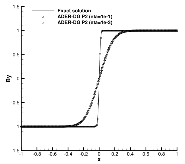
Figure 1: Current sheet at time $t=0.1$ simulated for different resistivities ($\eta=10^{-1}$ and $\eta=10^{-3}$) with the GPR model using an ADER-DG $P_{2}$ scheme.

7.3 Riemann problems

While the previous test cases involved only smooth solutions, the Riemann problems solved in this section contain all different kinds of elementary flow discontinuities. The initial conditions for density, velocity, pressure and magnetic field together with the final simulation time $t_{\textnormal{e}}$ as well as the position of the initial discontinuity $x_{d}$ are summarized in Table 2, while the initial data for the remaining variables are given by ${\bm{A}}=\sqrt[3]{\rho}\,\mathbf{I}$, $\mathbf{J}=0$ and $\mathbf{E}=-\mathbf{v}\times\mathbf{B}$. The computational domain is $\Omega=[-0.5,+0.5]\times[-0.1,0.1]$ and is discretized with an ADER-DG $P_{2}$ method using an adaptive Cartesian mesh (AMR) with initial resolution on the level zero grid of $100\times 4$ cells. Two levels of refinement are admitted ($\ell_{\max}=2$) with a refinement factor of $r=3$ between two adjacent levels. Refinement and recoarsening are based on the density as indicator variable. For more details on the AMR implementation, in particular for high order ADER schemes in combination with time-accurate local time stepping (LTS), see [32, 95]. The model parameters used for the simulation are $\gamma=\frac{5}{3}$, $\rho_{0}=1$, $c_{s}=0.8$, $\alpha^{2}=0.8$, $c=10$ and $\mu=\kappa=\eta=10^{-4}$, i.e. we are in a rather stiff regime of the model where a comparison with the ideal MHD equations is appropriate. The results obtained with the GPR model for density $\rho$ and the magnetic field component $B_{y}$ are depicted in Fig. 2 for all three problems, together with the exact solution of the Riemann problem of the ideal MHD equations. Overall, a good agreement can be noted, apart from the compound wave which can be observed in the density for RP1. This phenomenon is visible also in standard finite volume schemes applied to the ideal MHD equations, see e.g. [29].

Table 2: Initial states left and right for the density $\rho$, velocity vector $\mathbf{v}=(u,v,w)$, the pressure $p$ and the magnetic field vector $\mathbf{B}=(B_{x},B_{y},B_{z})$. The final output times, ($t_{\textnormal{end}}$) and the initial position of the discontinuity ($x_{d}$) are also given.

Case	$\rho$	$u$	$v$	$w$	$p$	$B_{x}$	$B_{y}$	$B_{z}$	$t_{\textnormal{e}}$, $x_{d}$
RP1 L:	1.0	0.0	0.0	0.0	1.0	$\frac{3}{4}$	$1$	0.0	0.1
R:	0.125	0.0	0.0	0.0	0.1	$\frac{3}{4}$	$-1$	0.0	0.0
RP2 L:	1.08	1.2	0.01	0.5	0.95	0.564189	1.015541	0.564189	0.2
R:	0.9891	-0.0131	0.0269	0.010037	0.97159	0.564189	1.135262	0.564923	-0.1
RP3 L:	1.0	0.0	0.0	0.0	1.0	$1.3$	$1$	0.0	0.16
R:	0.4	0.0	0.0	0.0	0.4	$1.3$	$-1$	0.0	0.0

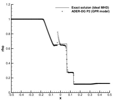
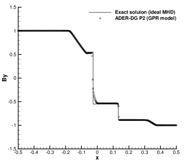
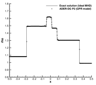
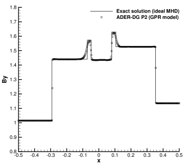
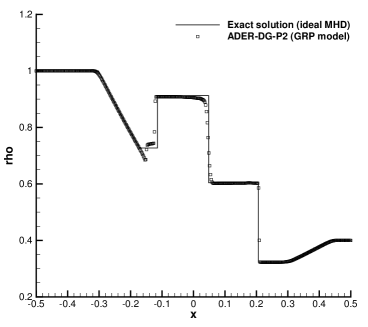
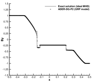
Figure 2: MHD Riemann problems RP1 (top), RP2 (center) and RP3 (bottom) simulated with the GPR model ($\mu=\kappa=\eta=10^{-4}$) using an ADER-DG $P_{2}$ scheme with AMR and comparison with the exact solution of the ideal MHD equations. The fluid density $\rho$ (left) and the magnetic field component $B_{y}$ (right) are depicted.

7.4 MHD rotor problem

Here we solve the well-known MHD rotor problem originally proposed by Balsara and Spicer in [3] and later also used in many other papers on numerical methods for the ideal MHD equations. In this test problem, a rapidly rotating high density fluid (the rotor) is embedded in a low density atmosphere at rest. The fluid pressure and the magnetic field are initially constant everywhere. The rotor produces torsional Alfvén waves which travel into the outer fluid. The computational domain is defined as $\Omega=[-0.5,+0.5]^{2}$ and we use an ADER-DG $P_{2}$ scheme on a uniform Cartesian grid composed of $200\times 200$ elements. The initial density is $\rho=10$ inside the rotor ($0\leq r\leq 0.1$) and $\rho=1$ for the outer fluid. The velocity in the outer fluid is initially set to zero, while it is given by $\mathbf{v}=\bm{\omega}\times\mathbf{x}$ inside the rotor, with $\bm{\omega}=(0,0,10)$. The initial pressure is $p=1$ and the magnetic field vector is set to $\mathbf{B}=(B_{0},0,0)^{T}$ in the entire computational domain $\Omega$, with $B_{0}=\frac{2.5}{\sqrt{4\pi}}$. As proposed by Balsara and Spicer, a linear taper is applied to the velocity and density field between $0.1\leq r\leq 0.105$. The other variables are initially set to ${\bm{A}}=\sqrt[3]{\rho}\,\mathbf{I}$, $\mathbf{J}=0$ and $\mathbf{E}=-\mathbf{v}\times\mathbf{B}$. The speed for the hyperbolic divergence cleaning is set to $c_{h}=2$ and the model parameters are $\gamma=1.4$, $c=10$, $\alpha^{2}=0.8$, $\rho_{0}=1$, $c_{s}=0.8$ and $\mu=\kappa=\eta=10^{-4}$, which make the system sufficiently stiff so that a comparison with the ideal MHD equations is possible. The results are depicted at time $t=0.25$ in Fig. 3 for the usual quantities density, pressure, Mach number and magnetic pressure. The results agree qualitatively well with those reported by Balsara and Spicer in [3], as well as those reported in other papers on high order numerical methods for the ideal MHD equations, see e.g. [24, 32].

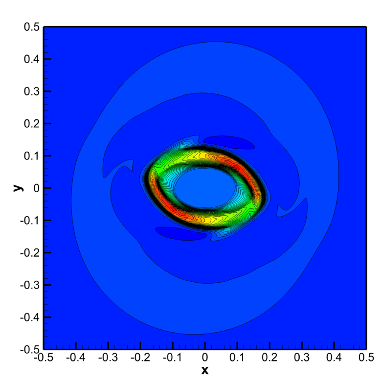
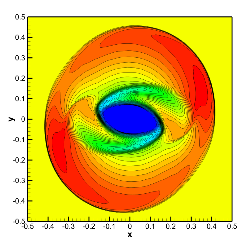
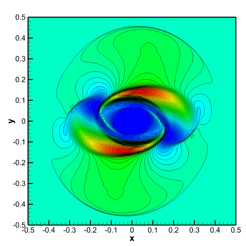
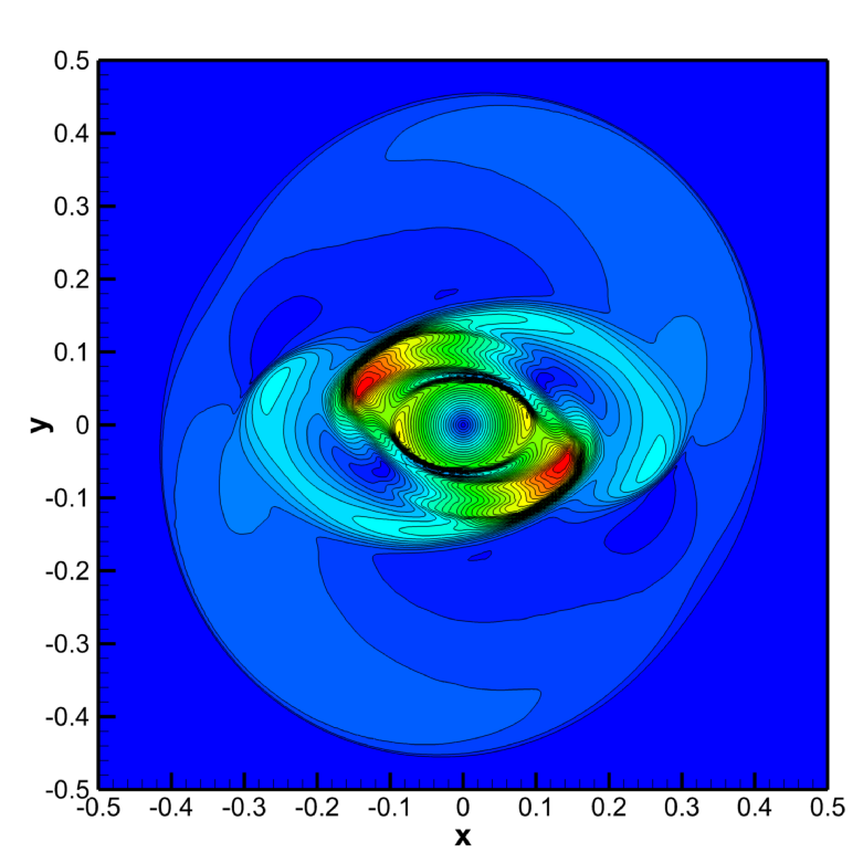
Figure 3: MHD rotor problem at time $t=0.25$ simulated with the GPR model ($\mu=\kappa=\eta=10^{-4}$) using an ADER-DG $P_{2}$ scheme. The contours of fluid density $\rho$ (top left), fluid pressure $p$ (top right), magnetic pressure (bottom left) and Mach number (bottom right) are shown.

7.5 MHD blast wave problem

The MHD blast wave problem is a very challenging test problem even for numerical schemes applied to the ideal MHD equations. Here, we solve the GPR model (72a)-(72g) in a rather stiff regime so that comparisons with numerical results obtained with the ideal MHD equations are possible. The computational domain is given by $\Omega=[-0.5,+0.5]^{2}$ and is discretized with an ADER-DG $P_{2}$ scheme on a uniform Cartesian grid using $200\times 200$ elements. The initial data are $\rho=1$, $\mathbf{v}=0$ and $\mathbf{B}=(B_{0},0,0)$ with $B_{0}=\frac{100}{\sqrt{4\pi}}$. The pressure is set to $p=1000$ in a small internal circular region ($r<0.1$) and is $p=0.1$ elsewhere, hence the pressure jumps over four orders of magnitude in this test problem. Furthermore, the fluid is highly magnetized due to the presence of a very strong magnetic field in the entire domain.

The other variables of the model are initially set to ${\bm{A}}=\sqrt[3]{\rho}\,\mathbf{I}$, $\mathbf{J}=0$ and $\mathbf{E}=-\mathbf{v}\times\mathbf{B}$. The speed for the hyperbolic divergence cleaning is chosen as $c_{h}=2$ and the model parameters are given by $\gamma=1.4$, $c=10$, $\alpha^{2}=0.8$, $\rho_{0}=1$, $c_{s}=0.8$ and $\mu=\kappa=\eta=10^{-3}$. The computational results are depicted at time $t=0.01$ in Fig. 4 for the magnetic field component $B_{x}$, the fluid pressure $p$, the density $\rho$ and the color map of the limited cells and unlimited cells in red and blue, respectively. For details on the finite volume subcell limiter, see [33, 95, 94]. The computational results agree qualitatively with those reported by Balsara and Spicer in [3].

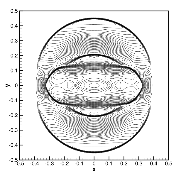
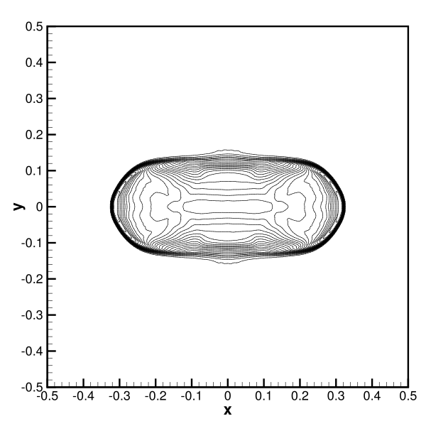
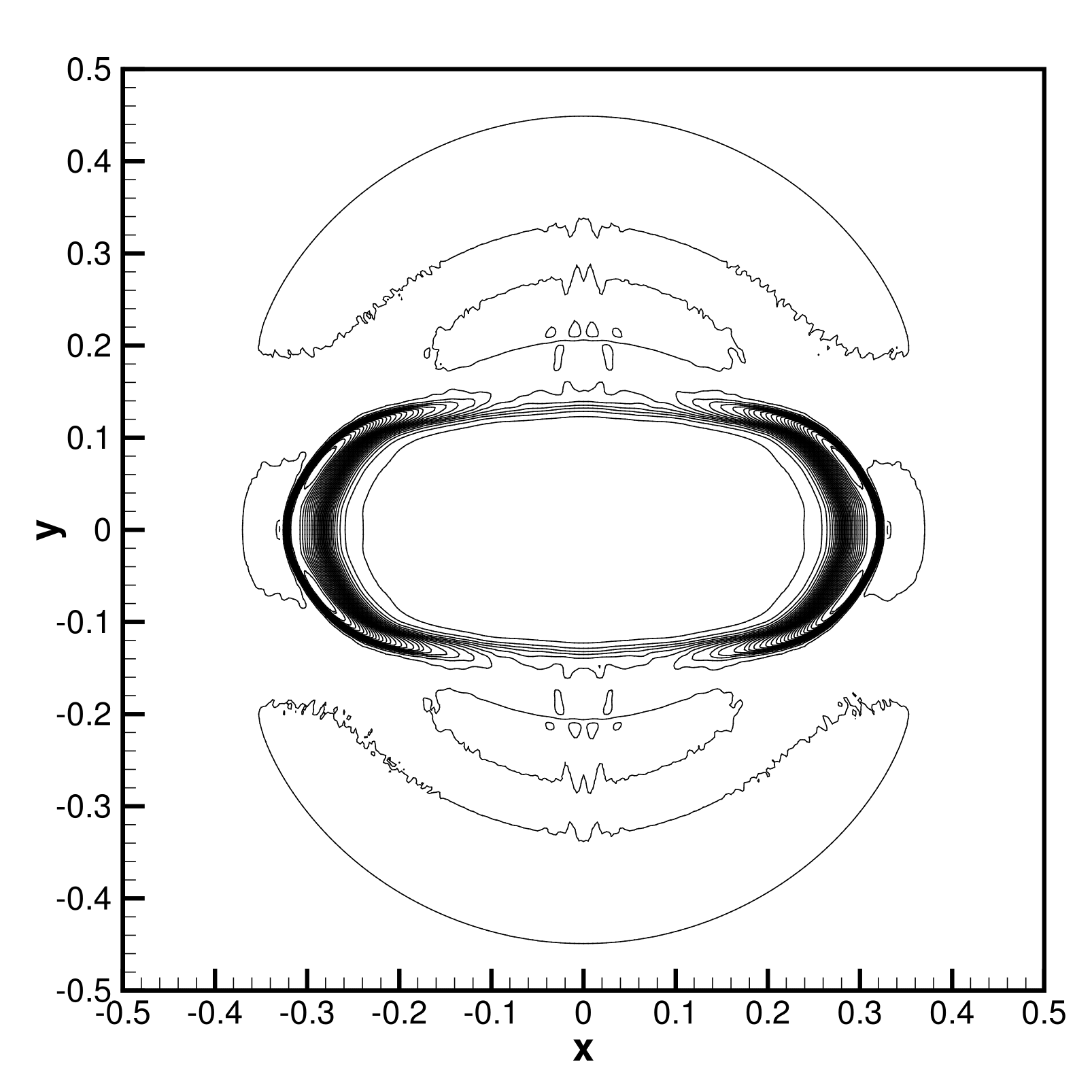
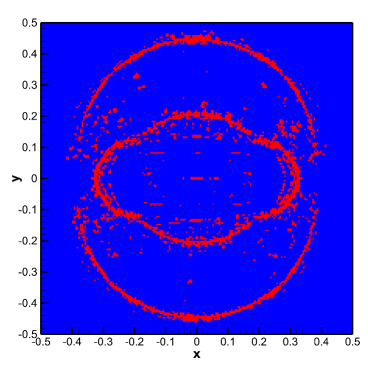
Figure 4: MHD blast wave problem at time $t=0.01$ using the GPR model ($\mu=\kappa=\eta=10^{-3}$) and an ADER-DG $P_{2}$ scheme. The contours of the magnetic field component $b_{x}$ (top left), the fluid pressure $p$ (top right) and the fluid density $\rho$ (bottom left) are shown, together with a map of troubled zones in red that use the subcell finite volume limiter of the ADER-DG $P_{2}$ scheme, while unlimited cells are colored in blue (bottom right).

7.6 Inviscid Orszag-Tang vortex system

In this section we study the well-known Orszag-Tang vortex system for the MHD equations [75, 19, 80], comparing the numerical results of the GPR model with those obtained with the ideal MHD equations. The setup is the one used in [58] and [24]. In both computations, the numerical method and the computational grid used are identical, as well as the initial conditions for the density, velocity, pressure and the magnetic field. The other variables of the GPR model are set to ${\bm{A}}=\sqrt[3]{\rho}\,\mathbf{I}$, $\mathbf{J}=0$ and $\mathbf{E}=-\mathbf{v}\times\mathbf{B}$. The computational domain under consideration is $\Omega=[0,2\pi]^{2}$ with four periodic boundary conditions and the initial conditions are given by $\rho=\gamma^{2}$, $\mathbf{v}=(-\sin(y),\sin(x),0)$, $p=\gamma$ and $\mathbf{B}=(-\sin(y),\sin(2x),0)$, with $\gamma=\frac{5}{3}$. The remaining parameters of the GPR model are $c=10$, $\alpha^{2}=0.8$, $c_{s}=0.8$, $c_{h}=2$, $\rho_{0}=1$ and $\mu=\kappa=\eta=10^{-4}$, so that the system is sufficiently stiff in order to allow a comparison with the ideal MHD equations. Simulations are carried out on a uniform Cartesian grid composed of $200\times 200$ elements using an ADER-DG $P_{2}$ scheme until a final time of $t=3$. The comparison between the computational results obtained with the GPR model and the ideal MHD equations is provided in Fig. 5. A very good agreement between the two solutions can be noted, even for later times when the solution has already developed many small scale structures. We stress that in both cases two completely different PDE systems have been solved.

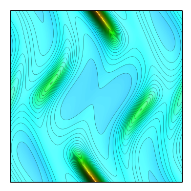
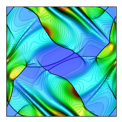
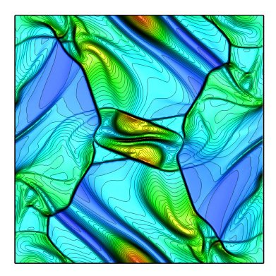
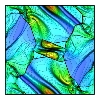
Figure 5: Orszag-Tang vortex problem at output times $t=0.5$, $t=2.0$ and $t=3.0$ from top to bottom. Left column: GPR model ($\mu=\kappa=\eta=10^{-4}$). Right column: ideal MHD equations for a direct comparison.

7.7 Viscous and resistive Orszag-Tang vortex

We now solve the Orszag-Tang vortex system in a highly viscous and resistive regime, where the computational results of the GPR model are compared with those of the viscous and resistive MHD equations (VRMHD). The computational setup of this test case is taken from [91] and [25], where also the governing PDE of the classical viscous and resistive MHD equations have been detailed. The computational domain is again $\Omega=[0,2\pi]^{2}$ with four periodic boundary conditions and the common initial condition for both models is given this time by $\rho=1$, $\mathbf{v}=(-\sin(y),\sin(x),0)$, $\mathbf{B}=(-\sin(y),\sin(2x),0)$, $p=\frac{15}{4}+\frac{1}{4}\cos(4x)+\frac{4}{5}\cos(2x)\cos(y)-\cos(x)\cos(y)+\frac{1}{4}\cos(2y)$. The ratio of specific heats is set to $\gamma=\frac{5}{3}$. The other variables of the GPR model are set to ${\bm{A}}=\mathbf{I}$, $\mathbf{J}=0$ and $\mathbf{E}=-\mathbf{v}\times\mathbf{B}$. We choose $\mu=\eta=10^{-2}$ and a Prandtl number of $Pr=1$ based on the heat capacity at constant volume of $c_{v}=1$, leading to a heat conduction coefficient of $\kappa=\gamma\mu$.

For the GPR model, we run the test problem until $t=2$ with an ADER-DG $P_{3}$ scheme on a uniform Cartesian grid composed of $200\times 200$ elements, while the numerical solution of the viscous and resistive MHD equations has been taken directly from [25], where an eighth order $P_{4}P_{7}$ scheme has been used to solve the VRMHD equations on a very coarse unstructured triangular mesh composed of only 990 triangles. The direct comparison between the first order hyperbolic GPR model and the second order hyperbolic-parabolic VRMHD model is provided in Fig. 6, where the velocity streamlines as well as the magnetic field lines are plotted. Overall, we can observe an excellent agreement between the two computational results, which have been obtained by solving two completely different PDE systems and using two different mesh topologies (Cartesian grid versus an unstructured simplex mesh).

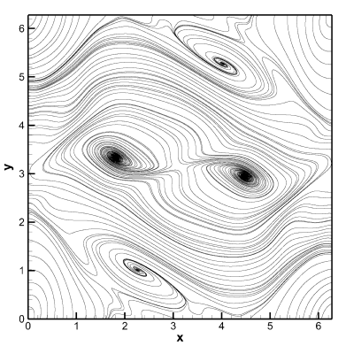
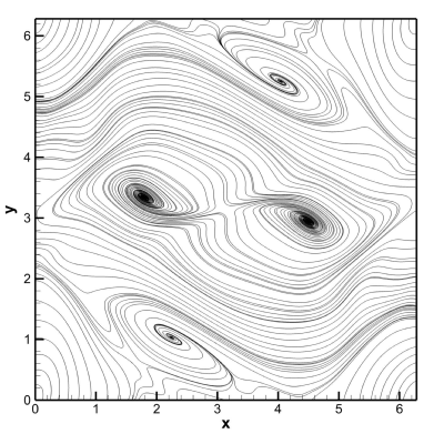
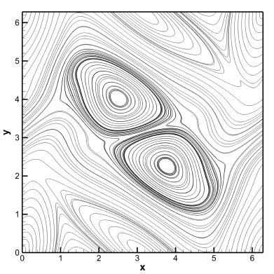
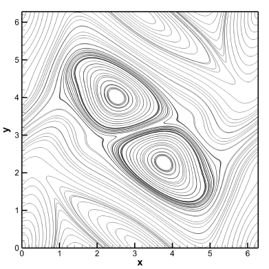
Figure 6: Viscous Orszag-Tang vortex problem ($\mu=\eta=10^{-2}$, $Pr=1$) at time $t=2.0$. First order hyperbolic GPR model (left) and classical VRMHD equations (right) for direct comparison. Velocity streamlines (top) and magnetic field lines (bottom).

7.8 Kelvin-Helmholtz instability in a viscous and resistive magnetized fluid

This test problem concerns the simulation of the Kelvin-Helmholtz instability in a magnetized fluid. As in the previous test, we solve the problem with the first order hyperbolic GPR model and with the viscous and resistive MHD equations (VRMHD). The setup of the initial conditions of the problem is taken from [25] and references therein: $\rho=1$, $p=\frac{3}{5}$, $\gamma=\frac{5}{3}$, $\mathbf{v}=(u,v,0)$ with $u=-\frac{1}{2}U_{0}\textnormal{tanh}\left(\frac{y-0.5}{a}\right)$ and $v=\delta v\sin(2\pi x)\sin(\pi y)$. The magnetic field is given by

$$\mathbf{B}=\left\{\begin{array}[]{ccc}(B_{0},0,0),&\textnormal{ if }&\frac{1}{2}+a<y<1,\\ (B_{0}\sin(\chi),0,B_{0}\cos(\chi)),&\textnormal{ if }&\frac{1}{2}-a<y<\frac{1}{2}+a,\\ (0,0,B_{0}),&\textnormal{ if }&0<y<\frac{1}{2}-a,\end{array}\right.$$

with $\chi=\frac{\pi}{2}\frac{y-0.5+a}{2a}$, $a=\frac{1}{25}$, $U_{0}=1$, $\delta v=0.01$ and $B_{0}=0.07$. The computational domain is $\Omega=[0,1]\times[-1,1]$ with periodic boundary conditions in the $x$ direction and is discretized with an ADER-DG $P_{2}$ scheme using $200\times 400$ elements for both PDE models, i.e. for the first order hyperbolic GPR system and for the viscous and resistive MHD model (VRMHD). The physical parameters are $\mu=\eta=10^{-3}$, $\kappa=0$, i.e. heat conduction is neglected in this test. The remaining parameters of the GPR model are set to $c=2$, $\alpha=0$, $c_{s}=0.8$, $c_{h}=2$ and $\rho_{0}=1$. The computational results are shown in Fig. 7, where an excellent agreement between the GPR results and the VRMHD results can be noted. One can clearly see the development of the so-called cat-eye vortices and the thin filaments connecting the individual vortices. For a detailed discussion of the MHD Kelvin-Helmholtz instability, see [60] and [57]. In Fig. 8 we also show two components of the distortion ${\bm{A}}$, which is the key quantity of the GPR model that allows the computation of the stress tensor in the case of both, fluids and solids. As already emphasized in [28], the distortion ${\bm{A}}$ is very well suited for flow visualization.

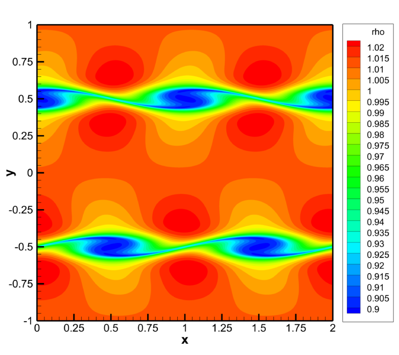
Figure 7: Kelvin-Helmholtz instability in a viscous and resistive magnetized fluid ($\mu=\eta=10^{-3}$, $\kappa=0$) at time $t=4.0$. Density contours obtained with an ADER-DG $P_{3}$ scheme for the first order hyperbolic GPR model (left) and for the VRMHD equations (right).

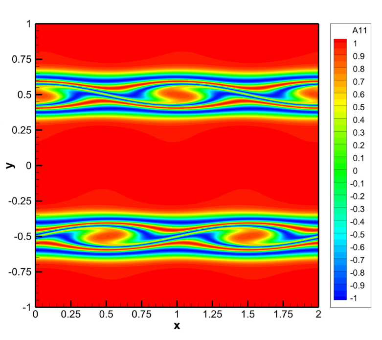
Figure 8: Kelvin-Helmholtz instability in a viscous and resistive magnetized fluid ($\mu=\eta=10^{-3}$, $\kappa=0$) at time $t=4.0$. Contours of the distortion components $A_{11}$ (left) and $A_{12}$ (right) for the first order hyperbolic GPR model.

7.9 High Lundquist number magnetic reconnection

As next test problem we consider the case of a high Lundquist number magnetic reconnection. Reconnection occurs in unstable current sheets due to the tearing instability that generates so-called plasmoid chains, see e.g. [11, 64, 87, 63]. For investigations of magnetic reconnection in the resistive relativistic case see [93], where high order ADER schemes similar to those employed in the present paper have been used [31].

The computational domain is given by $\Omega=[-25a,25a]\times[-L/2,L/2]$, where $L$ is the length of the domain, $a=L/S^{1/3}$ is the width of the current sheet and the Lundquist number is $S=Lv_{a}/\eta$, with the Alfvén speed $v_{a}$. The initial condition for the magnetic field is

$$\mathbf{B}=(0,B_{0}\textnormal{tanh}(x/a),B_{0}\textnormal{sech}(x/a)),$$ (132)

with the relation between $B_{0}$ and $v_{a}$ given by $v_{a}^{2}=B_{0}^{2}/\rho$. The initial fluid pressure is set to $p=\rho/(\gamma M^{2})$, where $M=v_{a}/c_{0}$ is the magnetic Mach number and $c_{0}$ is the sound speed. For our test we use $\rho=1$, $v_{a}=L=1$, $\gamma=5/3$, $M=0.7$ and $S=10^{6}$, hence the thickness of the current sheet is $a=0.01$, while the plasma parameter $\beta$ is given by $\beta=2.4$. The instability is triggered by adding a small perturbation to the velocity field of the form

$$u = \varepsilon\tanh\xi\exp(-\xi^{2})\cos(ky)$$ (133)

$$v = \varepsilon(2\xi\textnormal{tanh}\xi-\textnormal{sech}^{2}\xi)\exp(-\xi^{2})S^{1/2}\sin(ky)/k\,,$$ (134)

where $\varepsilon=10^{-3}$, $\xi=xS^{1/2}$ and the wave-number is computed from $kL=2\pi m$, with $m=10$. Free outflow and periodic boundary conditions are chosen along the $x$ and $y$ direction, respectively. The remaining variables and parameters of the GPR model are set to ${\bm{A}}=\sqrt[3]{\rho}\mathbf{I}$, $\mathbf{J}=0$, $\mathbf{E}=-\mathbf{v}\times\mathbf{B}$, $c=2$, $c_{h}=2$, $\rho_{0}=1$, $c_{s}=\alpha=0$, $\mu=\kappa=0$. Simulations have been carried out until a final time of $t=5.5$ using an ADER-DG $P_{2}$ scheme with a posteriori subcell finite volume limiter [33, 95, 94] on a uniform Cartesian grid composed of $200\times 400$ elements. In Fig. 9 the computational results for density, magnetic field component $B_{y}$ and for two components of the distortion ${\bm{A}}$ are shown. One can clearly see the formation of a main reconnection island or major plasmoid, which has the usual form similar to that observed also in other simulations reported in the literature [63, 35].

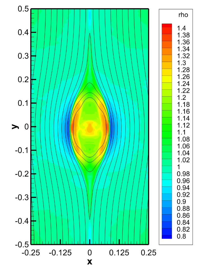
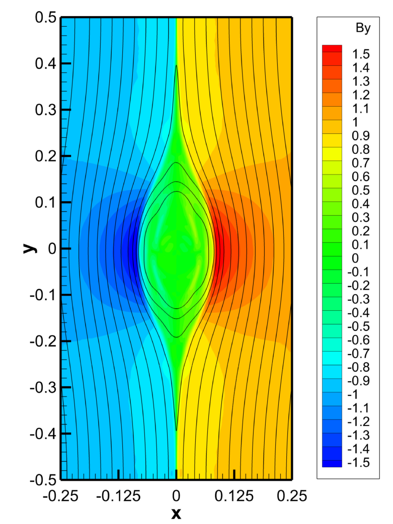
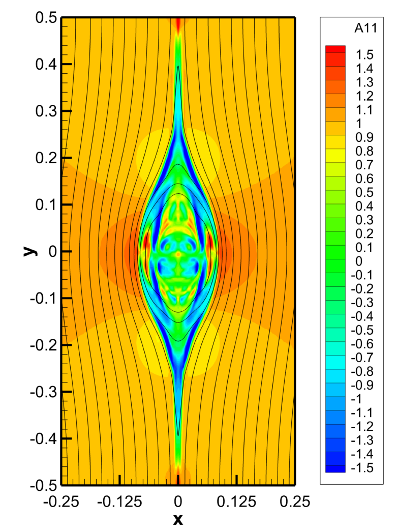
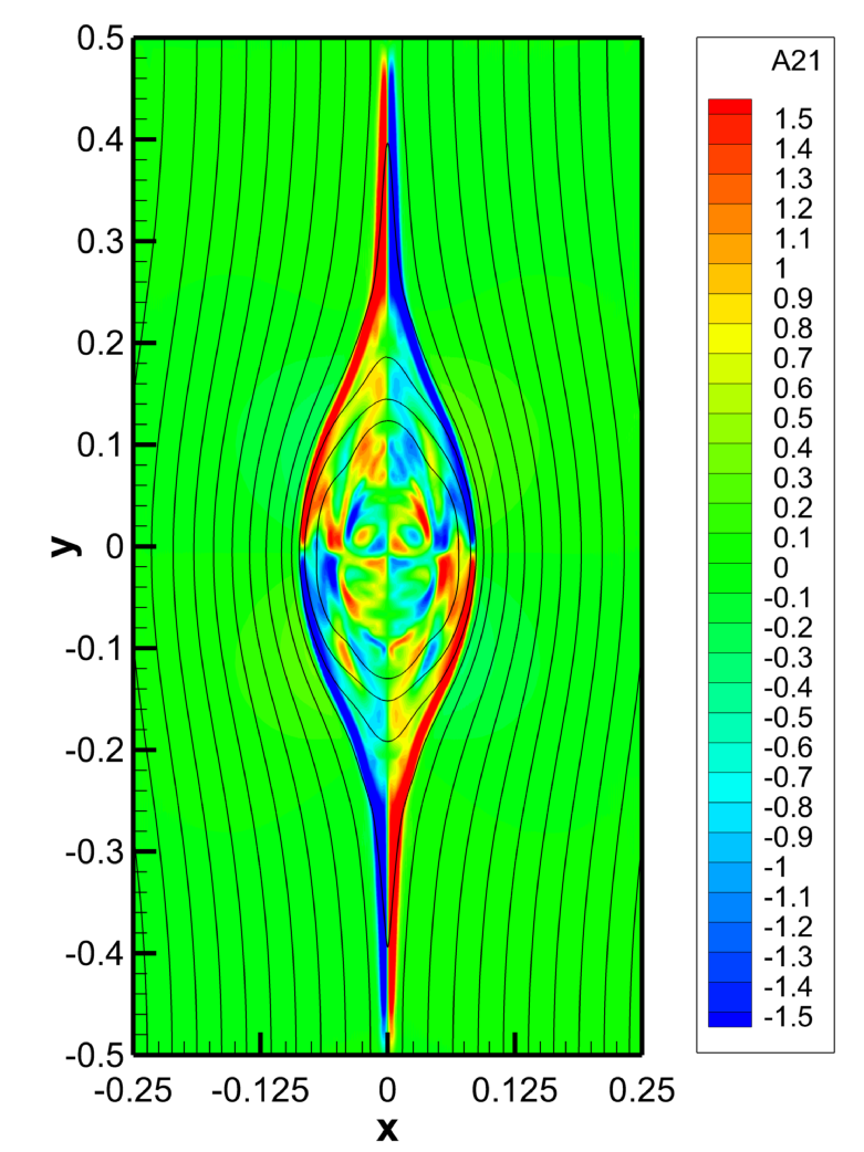
Figure 9: High Lundquist number magnetic reconnection ($\eta=10^{-6}$, $\mu=\kappa=0$) at time $t=5.5$. Results obtained for the first order hyperbolic GPR model with an ADER-DG $P_{2}$ scheme. Density (top left), magnetic field component $B_{y}$ (top right), distortion components $A_{11}$ (bottom left) and $A_{21}$ (bottom right). The magnetic field lines are also shown.

7.10 Scattering of a plane wave

Here, we run the GPR model inside a solid medium at rest in the limit $\tau_{1}\to\infty$, $\tau_{2}\to\infty$ and $\eta\to\infty$, i.e. without source terms. Hence, one expects to recover the behavior of the classical Maxwell equations concerning electromagnetic wave propagation. We therefore run the following test case twice, once with the full GPR model (72a)-(72g), and once with the standard time domain Maxwell equations in a laboratory frame at rest. For high order ADER-DG schemes applied to the Maxwell equations, see [89]. The computational domain for this test problem is $\Omega=[-2.5,+2.5]^{2}$ with four periodic boundary conditions. The initial electric and magnetic field vectors are set to $\mathbf{E}=(0,0,E_{0}\sin(kx))$ and $\mathbf{B}=(0,-B_{0}\sin(kx),0)$, with $k=4\pi$ and $E_{0}=B_{0}=0.1$, while the remaining variables of the GPR model are initially set to $\rho=1$, $p=1$, $\mathbf{v}=\mathbf{J}=0$ and ${\bm{A}}=\mathbf{I}$. The light speed is set to $c=c_{o}=1$ everywhere in $\Omega$, apart from a small cylindrical inclusion of radius $R=0.25$, where it has been set to $c=c_{i}=2$. In order to avoid spurious oscillations, the transition has been smoothed by setting $c(r)=c_{i}(1-\xi)+c_{o}\xi$, with $\xi=\frac{1}{2}(1+\textnormal{erf}((r-R)/\delta))$ and $\delta=0.05$. The remaining parameters in the GPR model are chosen as $\gamma=1.4$, $\tau_{1}=\tau_{2}=\eta=10^{20}$, $c_{h}=2$, $c_{s}=0.8$, $\alpha^{2}=0.8$ and $\rho_{0}=1$. The problem is run with an unlimited ADER-DG $P_{3}$ scheme on a uniform Cartesian grid composed of $100\times 100$ elements until a final time of $t=2.0$, so that the scattered waves have not yet reached the boundaries. In Fig. 10, the computational results obtained with the GPR model are compared to those of the standard Maxwell equations. Overall, a very good agreement can be noted between the two different models, both, for the contour plot of $B_{x}$ that represents the scattered wave field, as well as for the time series recorded in the four observation points $\mathbf{x}_{1}=(-1,0)$, $\mathbf{x}_{2}=(+1,0)$, $\mathbf{x}_{3}=(0,-1)$ and $\mathbf{x}_{4}=(0,+1)$.

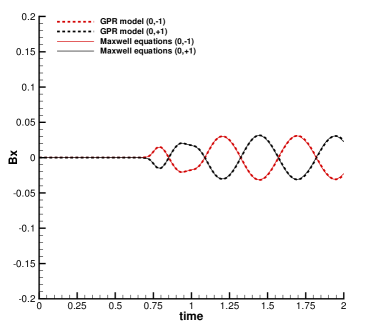
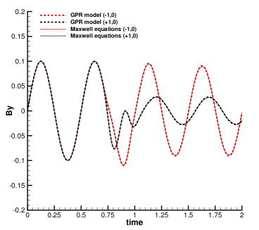
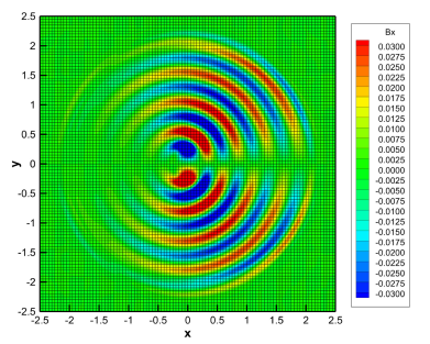
Figure 10: Scattering of a planar EM wave ($k=4\pi$) at a cylindrical inclusion of radius $R=0.25$. The light speed is $c=1$ in the ambient medium, while it is $c=2$ inside the inclusion. Comparison of the GPR model with the Maxwell equations using an ADER-DG $P_{3}$ scheme. Time series of the magnetic field components $B_{x}$ (top left) and $B_{y}$ (top right) registered in four observation points. Contour plot of the magnetic field component $B_{x}$ at time $t=2.0$ using the GPR model (bottom left) and the Maxwell equations (bottom right).

7.11 Comparison of different model regimes

In this last example we explore the behaviour of the GPR model in a large range of relaxation parameters, from the regime of a viscous and resistive magnetized fluid (case I, $\tau_{1}\ll 1$, $\tau_{2}\ll 1$, $\eta\ll 1$) over an electrically conducting elastic solid (case II, $\tau_{1}\to\infty$, $\tau_{2}\to\infty$, $\eta\ll 1$) to a non-conducting elastic solid (case III, $\tau_{1}\to\infty$, $\tau_{2}\to\infty$, $\eta\to\infty$). The initial data are essentially the same as for the MHD rotor problem solved in Section 7.4, i.e. density is set to $\rho=1$ in the ambient fluid and $\rho=10$ inside the rotor of radius $R=0.1$, while the initial pressure is constant everywhere $p=1$. The magnetic field vector is set to $\mathbf{B}=(B_{0},0,0)^{T}$ in the entire computational domain $\Omega$, with $B_{0}=\frac{2.5}{\sqrt{4\pi}}$ and the velocity is zero in the ambient fluid and $\mathbf{v}=\bm{\omega}\times\mathbf{x}$ inside the rotor, with $\bm{\omega}=(0,0,10)$. In this test we use a light speed of $c=4$ and the stiffened gas equation of state [28] with $p_{0}=1$. Furthermore, the reference density inside the rotor is chosen as $\rho_{0}=10$ so that the initial condition for the distortion is simply given by ${\bm{A}}=\mathbf{I}$. Furthermore, we initially set $\mathbf{J}=0$ and $\mathbf{E}=-\mathbf{v}\times\mathbf{B}$. The computational domain is $\Omega=[-1.25,+1.25]^{2}$, covered with a uniform Cartesian grid of $400\times 400$ elements. All simulations are carried out with a third order ADER-WENO finite volume scheme [32] and are run up to a final time of $t=0.25$. The parameters used for the three cases under consideration are summarized in Table 3.

Table 3: Relaxation parameters of the GPR model used for the three different cases under consideration ($c_{s}=0.8$, $\alpha^{2}=0.8$, $c=4$).

	Case I	Case II	Case III
	(viscous and resistive fluid)	(conducting elastic solid)	(non-conducting elastic solid)
$\tau_{1}$	$10^{-3}$	$10^{20}$	$10^{20}$
$\tau_{2}$	$10^{-3}$	$10^{20}$	$10^{20}$
$\eta$	$10^{-3}$	$10^{-3}$	$10^{20}$

The computational results are depicted in Fig. 11. We can see that in the case of electrically conducting material $\eta\ll 1$, the magnetic field is tight to the main pressure and shear waves arising in the medium, while in the case of an infinitely resistive or electrically non-conducting solid ($\eta\to\infty$), the electro-magnetic waves travel at the speed of light, independently of the other waves present in the medium. One can also clearly observe the effect of elasticity in the case of an elastic solid, since the rotor starts to oscillate and produce shear waves that are not visible in the case of the magnetized fluid, see the middle column of Fig. 11. A similar behavior of the velocity field in elastic bodies has already been observed in [24].

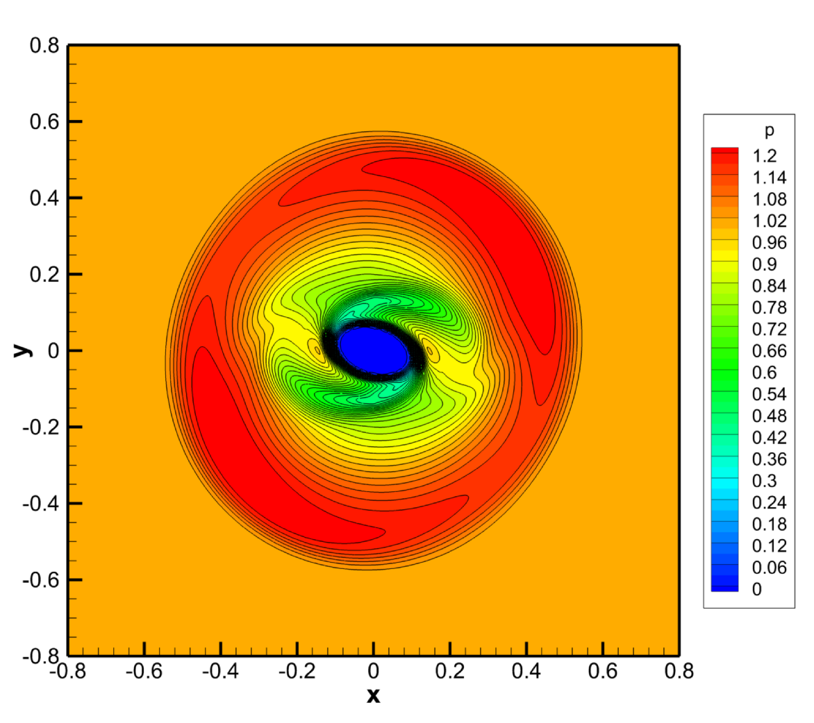
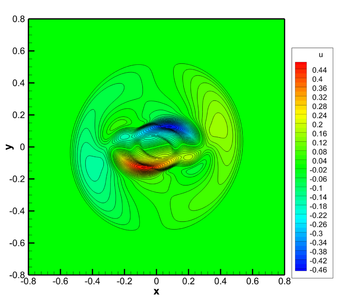
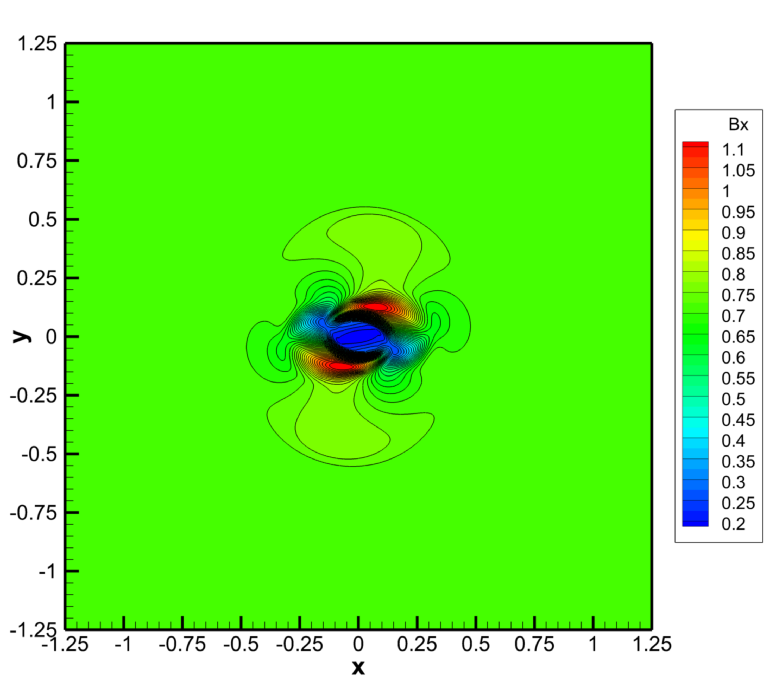
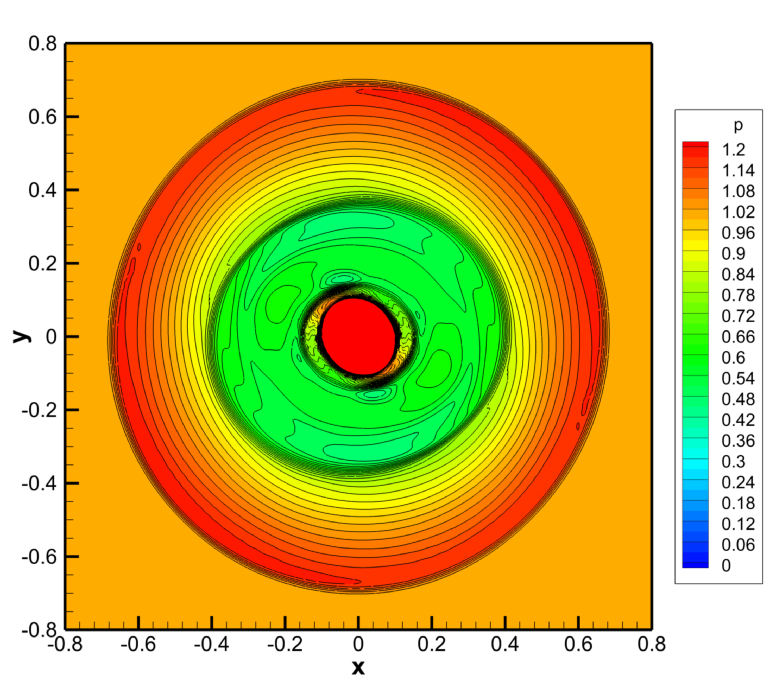
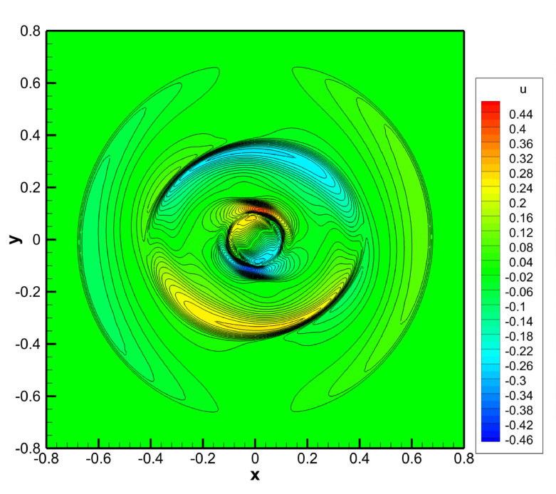
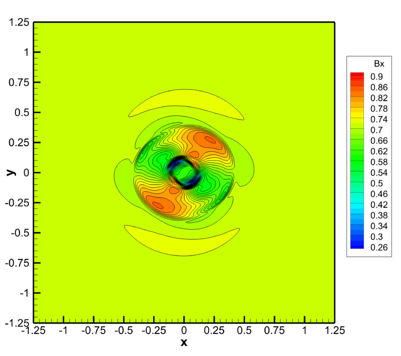
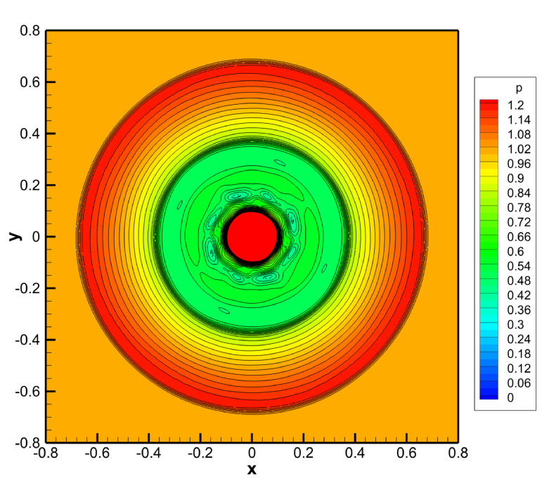
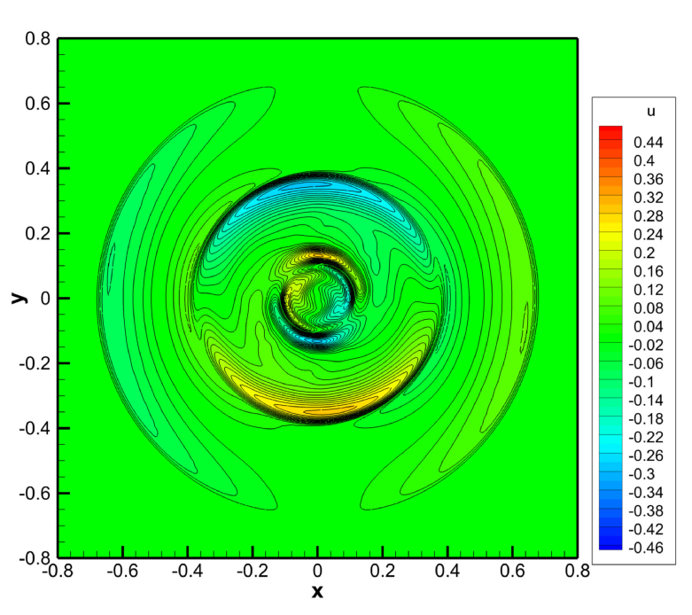
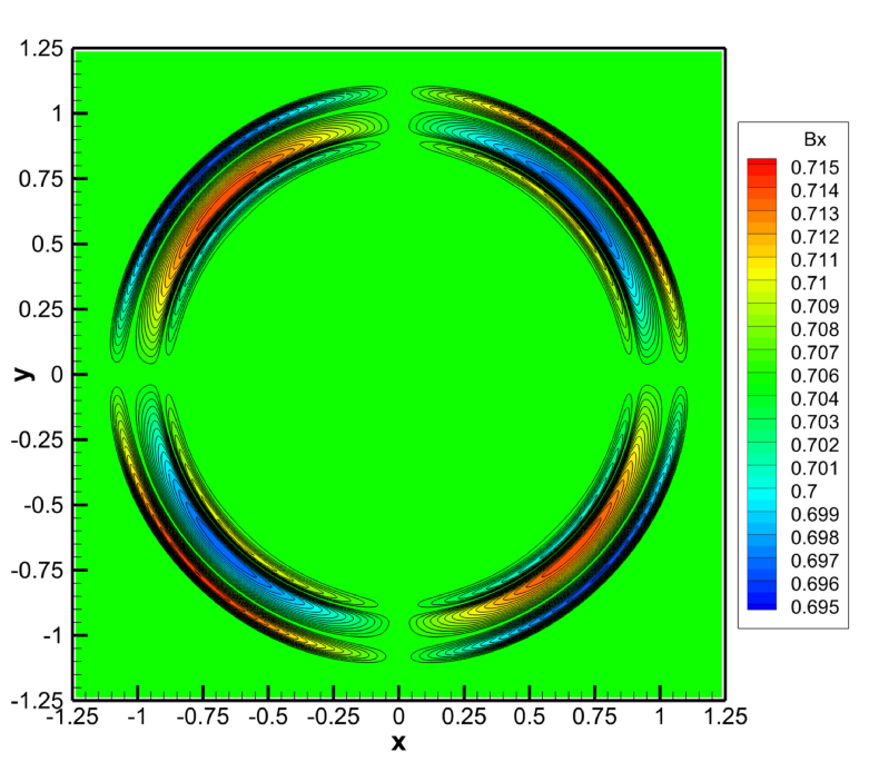
Figure 11: Rotor problem in different regimes of the relaxation parameters. Case I: viscous and resistive magnetized fluid (top row). Case II: magnetized electrically conducting elastic solid (middle row). Case III: magnetized electrically non-conducting elastic solid (bottom row). The contours of pressure (left column), velocity component $u$ (middle column) and magnetic field component $B_{x}$ are reported.

8 Conclusions

We have presented a new unified first order symmetric hyperbolic and thermodynamically compatible (HTC) model for the description of continuous media like fluids and solids interacting with electro-magnetic fields. The theoretical foundations of the model have been shown in great detail, in particular the connection of the final Eulerian form of model to the Euler-Lagrange differential equations associated with the underlying variational principle governed by the minimization of a Lagrangian. In the HTC framework, the dissipative terms are not modeled by classical parabolic differential operators (as for example in the Navier-Stokes or in the viscous and resistive MHD equations), but via algebraic relaxation source terms, like the Ohm law in the case of electro-magnetic wave propagation in conducting media. In the HTC framework, the same idea is also used to model dissipative momentum and heat transfer. The model satisfies the first and second principle of thermodynamics. It has also been shown via formal asymptotic analysis that in the stiff relaxation limit our first order hyperbolic system of PDEs reduces to the classical viscous and resistive MHD equations. A particular feature of the governing PDE system presented in this paper is the fact that all wave speeds remain finite, even in the stiff relaxation limit when the relaxation parameters $\tau_{1}$, $\tau_{2}$ and $\eta$ tend to zero. This makes the model a potential candidate for a possible future extension to the more general case of special and general relativistic continuum mechanics, in particular for the description of viscous and resistive relativistic fluids, where all propagation speeds in the medium must be necessarily bounded from above by the speed of light. In absence of relaxation source terms ($\tau_{1}\to\infty$, $\tau_{2}\to\infty$, $\eta\to\infty$), the PDE system proposed in this paper describes the propagation of electromagnetic waves in moving, electrically non-conducting dielectric media.

Future investigations will concern a more detailed study of the coupling between the stress tensor and the electro-magnetic field, as it appears, for example, in piezoelectric actuators. For that purpose, the coupling between the distortion and the electro-magnetic field needs to be considered within the generating potential. Further work is also needed concerning the development of new numerical methods which are able to preserve all stationary compatibility conditions, i.e. those on the matrix ${\bm{A}}$ and on the electro-magnetic fields exactly also at the discrete level. Finally, also the introduction of dispersive effects where the speed of propagation of electro-magnetic waves depends on the wave number will be subject to future research.

Appendix A Connection of the HTC model with the Maxwell equations

We start from the Maxwell equations in the laboratory frame, which are universally accepted to be true:

$$\frac{\partial{\mathbf{D}}}{\partial t}-\nabla\times{\mathbf{H}}=-{\mathbf{I}}$$ (135a)

$$\frac{\partial{\mathbf{B}}}{\partial t}+\nabla\times{\mathbf{E}}=0,$$ (135b)

with the constitutive relations

$${\mathbf{D}}=\epsilon^{\prime}{\mathbf{E}}\qquad\textnormal{ and }\qquad{\mathbf{B}}=\mu^{\prime}{\mathbf{H}}.$$ (136)

From (135) and (136) one obtains

$$\frac{\partial}{\partial t}\left(\epsilon^{\prime}{\mathbf{E}}\right)-\nabla\times{\mathbf{H}}=-{\mathbf{I}}$$ (137a)

$$\frac{\partial}{\partial t}\left(\mu^{\prime}{\mathbf{H}}\right)+\nabla\times{\mathbf{E}}=0,$$ (137b)

Here, $\mu^{\prime}=\mu_{0}\mu_{r}$ denotes the magnetic permeability of the medium (not to be confounded with the fluid viscosity $\mu$), given as a product of the magnetic permeability of vacuum $\mu_{0}$ and the relative permeability $\mu_{r}$. The electric permittivity is denoted by $\epsilon^{\prime}=\epsilon_{0}\epsilon_{r}$, where $\epsilon_{0}$ is the electric permittivity of vacuum and $\epsilon_{r}$ is the relative permittivity of the medium. In (135) the electric current ${\mathbf{I}}$ is given by the usual Ohm law

$${\mathbf{I}}=\rho_{c}{\mathbf{v}}+\sigma\left({\mathbf{E}}+{\mathbf{v}}\times{\mathbf{B}}\right),$$ (138)

with the conductivity $\sigma=1/\eta$ and the resistivity $\eta$. The charge density is $\rho_{c}=\epsilon^{\prime}\nabla\cdot{\mathbf{E}}$. We furthermore have the standard relation between the speed of light in the medium $c$, the magnetic permeability and the electric permittivity of the medium:

$$c^{2}=\frac{1}{\epsilon^{\prime}\mu^{\prime}}.$$ (139)

We now make the following change of variables

$${\mathbf{d}}={\mathbf{E}}+{\mathbf{v}}\times{\mathbf{B}},$$ (140a)

$${\mathbf{b}}={\mathbf{H}}-{\mathbf{v}}\times{\mathbf{D}}={\mathbf{H}}-\frac{{\mathbf{v}}\times{\mathbf{E}}}{\mu^{\prime}c^{2}}=\frac{1}{\mu^{\prime}}\left({\mathbf{B}}-\frac{{\mathbf{v}}\times{\mathbf{E}}}{c^{2}}\right),$$ (140b)

where ${\mathbf{d}}$ and ${\mathbf{b}}$ denote respectively the electric and the magnetic field in the comoving frame $K^{\prime}$ that moves with velocity ${\mathbf{v}}$. Substituting (140) into (135) yields

$$\frac{\partial}{\partial t}\left[\epsilon^{\prime}\left({\mathbf{d}}-{\mathbf{v}}\times{\mathbf{B}}\right)\right]-\nabla\times\left({\mathbf{b}}+\frac{{\mathbf{v}}\times{\mathbf{E}}}{\mu^{\prime}c^{2}}\right)=-\sigma{\mathbf{d}}-\epsilon^{\prime}{\mathbf{v}}\nabla\cdot{\mathbf{E}},$$ (141a)

$$\frac{\partial}{\partial t}\left[\mu^{\prime}\left({\mathbf{b}}+\frac{{\mathbf{v}}\times{\mathbf{E}}}{\mu^{\prime}c^{2}}\right)\right]+\nabla\times\left({\mathbf{d}}-{\mathbf{v}}\times{\mathbf{B}}\right)=0.$$ (141b)

We now substitute (140) also into the remaining terms of (141), hence obtaining

$$\frac{\partial}{\partial t}\left[\epsilon^{\prime}\left({\mathbf{d}}-{\mathbf{v}}\times\left(\mu^{\prime}{\mathbf{b}}+\frac{{\mathbf{v}}\times{\mathbf{E}}}{c^{2}}\right)\right)\right]+\nabla\times\left(-{\mathbf{b}}-\frac{{\mathbf{v}}\times({\mathbf{d}}-{\mathbf{v}}\times{\mathbf{B}})}{\mu^{\prime}c^{2}}\right)=-\sigma{\mathbf{d}}-\epsilon^{\prime}{\mathbf{v}}\nabla\cdot{\mathbf{E}},$$ (142a)

$$\frac{\partial}{\partial t}\left[\mu^{\prime}\left({\mathbf{b}}+\frac{{\mathbf{v}}\times\left({\mathbf{d}}-{\mathbf{v}}\times{\mathbf{B}}\right))}{\mu^{\prime}c^{2}}\right)\right]+\nabla\times\left(\phantom{-}{\mathbf{d}}-{\mathbf{v}}\times\left(\mu^{\prime}{\mathbf{b}}+\frac{{\mathbf{v}}\times{\mathbf{E}}}{c^{2}}\right)\right)=0.$$ (142b)

The above equations are still fully consistent with the relativistic equations; no assumptions have been made so far, only a change of variables. The formal structure is still exactly the same as the one of the original Maxwell equations (135). We now insert (140) once more into the fluxes of (142), which yields

$$\frac{\partial}{\partial t}\left[\epsilon^{\prime}\left({\mathbf{d}}-{\mathbf{v}}\times\left(\mu^{\prime}{\mathbf{b}}+\frac{{\mathbf{v}}\times{\mathbf{E}}}{c^{2}}\right)\right)\right]+\nabla\times\left(-{\mathbf{b}}-\frac{{\mathbf{v}}\times\left({\mathbf{d}}-{\mathbf{v}}\times\left(\mu^{\prime}{\mathbf{b}}+\frac{{\mathbf{v}}\times{\mathbf{E}}}{c^{2}}\right)\right)}{\mu^{\prime}c^{2}}\right)=-\sigma{\mathbf{d}}-\epsilon^{\prime}{\mathbf{v}}\nabla\cdot{\mathbf{E}},$$ (143a)

$$\frac{\partial}{\partial t}\left[\mu^{\prime}\left({\mathbf{b}}+\frac{{\mathbf{v}}\times\left({\mathbf{d}}-{\mathbf{v}}\times{\mathbf{B}}\right))}{\mu^{\prime}c^{2}}\right)\right]+\nabla\times\left(\phantom{-}{\mathbf{d}}-{\mathbf{v}}\times\left(\mu^{\prime}{\mathbf{b}}+\frac{{\mathbf{v}}\times\left({\mathbf{d}}-{\mathbf{v}}\times{\mathbf{B}}\right)}{c^{2}}\right)\right)=0.$$ (143b)

With the auxiliary variables

$${\mathbf{e}}^{\prime}:=\epsilon^{\prime}\left({\mathbf{d}}-{\mathbf{v}}\times\left(\mu^{\prime}{\mathbf{b}}+\frac{{\mathbf{v}}\times{\mathbf{E}}}{c^{2}}\right)\right)=\epsilon^{\prime}\left({\mathbf{d}}-\mu^{\prime}{\mathbf{v}}\times{\mathbf{b}}-\frac{1}{c^{2}}{\mathbf{v}}\times\left({\mathbf{v}}\times{\mathbf{E}}\right)\right),$$ (144a)

$${\mathbf{h}}^{\prime}:=\mu^{\prime}{\mathbf{b}}+\frac{{\mathbf{v}}\times\left({\mathbf{d}}-{\mathbf{v}}\times{\mathbf{B}}\right)}{c^{2}}=\mu^{\prime}{\mathbf{b}}+\frac{{\mathbf{v}}\times{\mathbf{d}}}{c^{2}}-\frac{1}{c^{2}}{\mathbf{v}}\times\left({\mathbf{v}}\times{\mathbf{B}}\right),$$ (144b)

the system (143) can be rewritten as

$$\frac{\partial{\mathbf{e}}^{\prime}}{\partial t}+\nabla\times\left(-{\mathbf{v}}\times{\mathbf{e}}^{\prime}-{\mathbf{b}}\right)=-\sigma{\mathbf{d}}-\epsilon^{\prime}{\mathbf{v}}\nabla\cdot{\mathbf{E}},$$ (145a)

$$\frac{\partial{\mathbf{h}}^{\prime}}{\partial t}+\nabla\times\left(-{\mathbf{v}}\times{\mathbf{h}}^{\prime}+{\mathbf{d}}\right)=0.$$ (145b)

We now assume that ${\mathbf{v}}^{2}/c^{2}\ll 1$, hence we neglect quadratic terms in ${\mathbf{v}}/c$. This allows us to define the new simplified conserved variables

$${\mathbf{e}}:=\epsilon^{\prime}{\mathbf{d}}-\epsilon^{\prime}\mu^{\prime}{\mathbf{v}}\times{\mathbf{b}}\approx{\mathbf{e}}^{\prime},$$ (146a)

$${\mathbf{h}}:=\mu^{\prime}{\mathbf{b}}+\epsilon^{\prime}\mu^{\prime}{\mathbf{v}}\times{\mathbf{d}}\approx{\mathbf{h}}^{\prime},$$ (146b)

which yields the following simplified system, where we have also used the identity $\nabla\cdot{\mathbf{B}}=0$ and where again quadratic terms in ${\mathbf{v}}/c$ have been neglected in the final expressions:

$$\frac{\partial{\mathbf{e}}}{\partial t}+\nabla\times\left(-{\mathbf{v}}\times{\mathbf{e}}-{\mathbf{b}}\right)+{\mathbf{v}}\,\nabla\cdot{\mathbf{e}}=-\sigma{\mathbf{d}},$$ (147a)

$$\frac{\partial{\mathbf{h}}}{\partial t}+\nabla\times\left(-{\mathbf{v}}\times{\mathbf{h}}+{\mathbf{d}}\right)+{\mathbf{v}}\,\nabla\cdot{\mathbf{h}}=0.$$ (147b)

The above system is written in the form given in [84]. Note that compared to [84], the consistency with the Maxwell equations in the laboratory frame requires the following definition of the generating potential for electro-magnetic energy density:

$$L_{em}=\frac{1}{2}\left(\mu^{\prime}{\mathbf{b}}^{2}+\epsilon^{\prime}{\mathbf{d}}^{2}\right)+\epsilon^{\prime}\mu^{\prime}{\mathbf{v}}\cdot({\mathbf{d}}\times{\mathbf{b}})=\frac{1}{2}\left(\mu^{\prime}b_{i}b_{i}+\epsilon^{\prime}d_{i}d_{i}\right)+\epsilon^{\prime}\mu^{\prime}\,\varepsilon_{ijk}v_{i}d_{j}b_{k},$$ (148)

since we must have that

$$e_{i}=\frac{\partial L_{em}}{\partial d_{i}}=\epsilon^{\prime}d_{i}-\epsilon^{\prime}\mu^{\prime}\,\varepsilon_{ijk}v_{j}b_{k},$$ (149)

$$h_{i}=\frac{\partial L_{em}}{\partial b_{i}}=\mu^{\prime}b_{i}+\epsilon^{\prime}\mu^{\prime}\,\varepsilon_{ijk}v_{j}d_{k}.$$ (150)

Using (146) and (140) the variables ${\mathbf{e}}$ and ${\mathbf{h}}$ can be expressed in terms of the electro-magnetic field quantities in the laboratory frame as follows:

$${\mathbf{e}}=\epsilon^{\prime}\left({\mathbf{E}}+\frac{1}{c^{2}}{\mathbf{v}}\times{\mathbf{v}}\times{\mathbf{E}}\right),\qquad\textnormal{ and }\qquad{\mathbf{h}}=\mu^{\prime}{\mathbf{H}}+\frac{1}{c^{2}}{\mathbf{v}}\times{\mathbf{v}}\times{\mathbf{E}},$$ (151)

which together with (136) reduces to the simple identities

$${\mathbf{e}}={\mathbf{D}},\qquad\textnormal{ and }\qquad{\mathbf{h}}={\mathbf{B}},$$ (152)

if quadratic terms in ${\mathbf{v}}/c$ are again neglected in (151).

Appendix B Euler-to-Lagrange field transformation

In this section, we demonstrate how to obtain Eulerian equations (35d)–(35e) for electromagnetic fields $e_{i}$ and $h_{i}$ from their Lagrangian counterparts (16c)–(16d). However, it is more convenient to chose the opposite strategy. Namely, we derive the Lagrangian field equations from the Eulerian. Thus, if one likes to get the Lagrange-to-Euler derivation then the calculations should be repeated from the end to the beginning of what follows. Recall that in (16c)–(16d) we use the same notations $e_{i}$ and $h_{i}$ for the fields however they are different. As we mentioned earlier and as will be proven in what follows, the Eulerian and Lagrangian fields are related by (38). As discussed in Section 2, in the structure study, we can ignore the algebraic source terms as they are low order terms.

B.1 Auxiliary relations

Here, we summarize the definitions and formulas used in this section. The total deformation gradient ${\bm{F}}=[F_{ij}]$, the distortion matrix ${\bm{A}}=[A_{ij}]$ and the velocity are defined as

$$F_{ij}=\dfrac{\mathcal{\partial}x_{i}}{\mathcal{\partial}y_{j}},\qquad{\bm{A}}={\bm{F}}^{-1},\qquad w=\det({\bm{F}})=\dfrac{\rho_{0}}{\rho},\qquad v_{i}=\frac{{\rm d}x_{i}}{{\rm d}t},$$ (153)

where, as previously, $y_{j}$ are the Lagrangian coordinates and $x_{i}$ are the Eulerian ones, $\rho$ and $\rho_{0}$ are the actual and the reference mass densities, respectively. The time evolution equation for $F_{ij}$ in the Lagrangian coordinates

$$\frac{{\rm d}F_{ij}}{{\rm d}t}-\frac{\mathcal{\partial}v_{i}}{\mathcal{\partial}y_{j}}=0$$ (154)

is a trivial consequence of definitions (153).

The following standard definitions and formulas are also introduced

$$\bm{C}={\rm cof}({\bm{F}})=w{\bm{A}}^{\mathsf{T}}=\left[C_{{ij}}\right],{\ \rm\ \ or\ \ }A_{{ij}}=w^{-1}C_{{ji}},$$ (155)

$$\frac{\partial C_{ij}}{\partial y_{j}}=0,\qquad\varepsilon_{{mjp}}\frac{\partial F_{{mp}}}{\partial y_{j}}=0,$$ (156)

$$\frac{{\rm d}w}{{\rm d}t}-\frac{\partial wA_{jk}v_{k}}{\partial y_{j}}=0,{\rm or\ using\ (\ref{eq.CofDefinition})\ and\ (\ref{eq.DivCof}):\ \ \ }\frac{{\rm d}w}{{\rm d}t}-wA_{jk}\frac{\partial v_{k}}{\partial y_{j}}=0,$$ (157)

$$\varepsilon_{{ikl}}A_{{mi}}A_{{jk}}A_{{al}}=\varepsilon_{mja}w^{-1},$$ (158)

$$C_{{km}}=\frac{1}{2}\varepsilon_{{lnk}}\varepsilon_{{pqm}}F_{{lp}}F_{{nq}},$$ (159)

$$\varepsilon_{{imn}}\varepsilon_{{jmn}}=2\delta_{{ij}}.$$ (160)

B.2 Transformation of (35d)–(35e) to (16c)–(16d)

We shall transform (35d) into (16c) while (35e) transforms into (16d) analogously. Thus, (35d) is equivalent to

$$\frac{\partial e_{i}}{\partial t}+v_{k}\frac{\partial e_{i}}{\partial x_{k}}+\frac{\partial v_{k}}{\partial x_{k}}e_{i}-\frac{\partial v_{i}}{\partial x_{k}}e_{k}-\varepsilon_{{ikl}}\frac{\partial{\mathcal{E}}_{h_{l}}}{\partial x_{k}}=0.$$ (161)

Using ${\rm d}/{{\rm d}t}=\partial/\partial t+v_{k}/\partial x_{k}$ we have

$$\frac{{\rm d}e_{i}}{{{\rm d}t}}+\frac{\partial v_{k}}{\partial x_{k}}e_{i}-\frac{\partial v_{i}}{\partial x_{k}}e_{k}-\varepsilon_{{ikl}}\frac{\partial{\mathcal{E}}_{h_{l}}}{\partial x_{k}}=0.$$ (162)

From (153) it follows that $\frac{\mathcal{\partial}}{\mathcal{\partial}x_{k}}=A_{{jk}}\frac{\mathcal{\partial}}{\mathcal{\partial}y_{j}}$ and thus we change the variables $x_{k}$ on $y_{j}$

$$\frac{{\rm d}e_{i}}{{{\rm d}t}}+A_{{jk}}\frac{\partial v_{k}}{\partial y_{j}}e_{i}-A_{{jk}}\frac{\partial v_{i}}{\partial y_{j}}e_{k}-\varepsilon_{{ikl}}A_{{jk}}\frac{\partial{\mathcal{E}}_{h_{l}}}{\partial y_{j}}=0.$$ (163)

Applying (157)₂ to the second term and (154) to the third term of the last equation, we have

$$\frac{{\rm d}e_{i}}{{{\rm d}t}}+\frac{1}{w}\frac{{{\rm d}w}}{{{\rm d}t}}e_{i}-A_{{jk}}\frac{{\rm d}F_{ij}}{{\rm d}t}e_{k}-\varepsilon_{{ikl}}A_{{jk}}\frac{\partial E_{h_{l}}}{\partial y_{j}}=0,$$ (164)

$$\frac{{\rm d}we_{i}}{{{\rm d}t}}-we_{k}A_{{jk}}\frac{{\rm d}F_{ij}}{{\rm d}t}-w\varepsilon_{{ikl}}A_{{jk}}\frac{\partial{\mathcal{E}}_{h_{l}}}{\partial y_{j}}=0,$$ (165)

Now, we add $0\equiv we_{k}\dfrac{{\rm d}\delta_{ik}}{{\rm d}t}$ to the left hand side and then using that $\delta_{ik}=F_{ij}A_{jk}$ one can obtain that

$$\frac{{\rm d}we_{i}}{{{\rm d}t}}+we_{k}\frac{{\rm d}\delta_{ik}}{{\rm d}t}-we_{k}A_{{jk}}\frac{{{\rm d}F}_{{ij}}}{{{\rm d}t}}-w\varepsilon_{{ikl}}A_{{jk}}\frac{\partial{\mathcal{E}}_{h_{l}}}{\partial y_{j}}=0,$$ (166)

$$\frac{{\rm d}we_{i}}{{{\rm d}t}}+we_{k}\frac{{\rm d}F_{{ij}}A_{{jk}}}{{{\rm d}t}}-we_{k}A_{{jk}}\frac{{{\rm d}F}_{{ij}}}{{{\rm d}t}}-w\varepsilon_{{ikl}}A_{{jk}}\frac{\partial{\mathcal{E}}_{h_{l}}}{\partial y_{j}}=0,$$ (167)

$$\frac{{\rm d}we_{i}}{{{\rm d}t}}+we_{k}F_{{ij}}\frac{{\rm d}A_{{jk}}}{{{\rm d}t}}+we_{k}\frac{{\rm d}F_{{ij}}}{{{\rm d}t}}A_{{jk}}-we_{k}A_{{jk}}\frac{{{\rm d}F}_{{ij}}}{{{\rm d}t}}-w\varepsilon_{{ikl}}A_{{jk}}\frac{\partial{\mathcal{E}}_{h_{l}}}{\partial y_{j}}=0.$$ (168)

After multiplying the last equation by $A_{mi}$

$$A_{{mi}}\left(\frac{{\rm d}we_{i}}{{{\rm d}t}}+we_{k}F_{{ij}}\frac{{\rm d}A_{{jk}}}{{{\rm d}t}}-w\varepsilon_{{ikl}}A_{{jk}}\frac{\partial{\mathcal{E}}_{h_{l}}}{\partial y_{j}}\right)=0,$$ (169)

$$A_{{mi}}\frac{{\rm d}we_{i}}{{{\rm d}t}}+we_{k}\frac{{\rm d}A_{{mk}}}{{{\rm d}t}}-w\varepsilon_{{ikl}}A_{{mi}}A_{{jk}}\frac{\partial{\mathcal{E}}_{h_{l}}}{\partial y_{j}}=0,$$ (170)

we have an intermediate result:

$$\frac{{\rm d}wA_{{mk}}e_{k}}{{{\rm d}t}}-w\varepsilon_{{ikl}}A_{{mi}}A_{{jk}}\frac{\partial{\mathcal{E}}_{h_{l}}}{\partial y_{j}}=0.$$ (171)

Now, we introduce the change of unknowns (38): $wA_{{mk}}e_{k}=e^{\prime}_{m}$, $wA_{{mk}}h_{k}=h^{\prime}_{m}$, and we also change the energy potential ${\mathcal{E}}(e_{i},h_{i})={\mathcal{E}}(w^{-1}F_{{ij}}e^{\prime}_{j},w^{-1}F_{{ij}}h^{\prime}_{j})=w^{-1}U(e^{\prime}_{j},h^{\prime}_{j})$. Hence, ${\mathcal{E}}_{h_{i}}=A_{ji}U_{h^{\prime}_{j}}$. After this, the intermediate result (171) reads as

$$\frac{{\rm d}e^{\prime}_{m}}{{{\rm d}t}}-w\varepsilon_{{ikl}}A_{{mi}}A_{{jk}}\frac{\partial A_{{al}}U_{h^{\prime}_{a}}}{\partial y_{j}}=0,$$ (172)

$$\frac{{\rm d}e^{\prime}_{m}}{{{\rm d}t}}-w\varepsilon_{{ikl}}A_{{mi}}A_{{jk}}A_{{al}}\frac{\partial U_{h^{\prime}_{a}}}{\partial y_{j}}-w\varepsilon_{{ikl}}A_{{mi}}A_{{jk}}\frac{\partial A_{{al}}}{\partial y_{j}}U_{h^{\prime}_{a}}=0.$$ (173)

Applying (158) and (155)₃ to the second term, we get

$$\frac{{\rm d}e^{\prime}_{m}}{{{\rm d}t}}-\varepsilon_{{mja}}\frac{\partial U_{h^{\prime}_{a}}}{\partial y_{j}}-w\varepsilon_{{ikl}}A_{{mi}}A_{{jk}}\frac{\partial A_{{al}}}{\partial y_{j}}U_{h^{\prime}_{a}}=0,$$ (174)

Now using the cofactor definition (155) and then applying (159) to the third term, we have

$$\frac{{\rm d}e^{\prime}_{m}}{{{\rm d}t}}-\varepsilon_{{mja}}\frac{\partial U_{h^{\prime}_{a}}}{\partial y_{j}}-\varepsilon_{{ikl}}A_{{mi}}C_{{kj}}\frac{\partial A_{{al}}}{\partial y_{j}}U_{h^{\prime}_{a}}=0,$$ (175)

$$\frac{{\rm d}e^{\prime}_{m}}{{{\rm d}t}}-\varepsilon_{{mja}}\frac{\partial U_{h^{\prime}_{a}}}{\partial y_{j}}-\frac{1}{2}\varepsilon_{{ikl}}\varepsilon_{{lnk}}\varepsilon_{{pqj}}F_{{lp}}F_{{nq}}A_{{mi}}\frac{\partial A_{{al}}}{\partial y_{j}}U_{h^{\prime}_{a}}=0.$$ (176)

Using (160) in the third term gives us

$$\frac{{\rm d}e^{\prime}_{m}}{{{\rm d}t}}-\varepsilon_{{mja}}\frac{\partial U_{h^{\prime}_{a}}}{\partial y_{j}}-\delta_{{in}}\varepsilon_{{pqj}}F_{{lp}}F_{{nq}}A_{{mi}}\frac{\partial A_{{al}}}{\partial y_{j}}U_{h^{\prime}_{a}}=0,$$ (177)

and subsequently,

$$\frac{{\rm d}e^{\prime}_{m}}{{{\rm d}t}}-\varepsilon_{{mja}}\frac{\partial U_{h^{\prime}_{a}}}{\partial y_{j}}-\varepsilon_{{pqj}}F_{{lp}}F_{{iq}}A_{{mi}}\frac{\partial A_{{al}}}{\partial y_{j}}U_{h^{\prime}_{a}}=0,$$ (178)

$$\frac{{\rm d}e^{\prime}_{m}}{{{\rm d}t}}-\varepsilon_{{mja}}\frac{\partial U_{h^{\prime}_{a}}}{\partial y_{j}}-\varepsilon_{{mjp}}F_{{lp}}\frac{\partial A_{{al}}}{\partial y_{j}}U_{h^{\prime}_{a}}=0.$$ (179)

Now, adding $0\equiv\varepsilon_{{mjp}}\frac{\partial F_{{lp}}}{\partial y_{j}}A_{{al}}U_{h^{\prime}_{a}}$ (see (156)₂), we get

$$\frac{{\rm d}e^{\prime}_{m}}{{{\rm d}t}}-\varepsilon_{{mja}}\frac{\partial U_{h^{\prime}_{a}}}{\partial y_{j}}-\varepsilon_{{mjp}}F_{{lp}}\frac{\partial A_{{al}}}{\partial y_{j}}U_{h^{\prime}_{a}}-\varepsilon_{{mjp}}\frac{\partial F_{{lp}}}{\partial y_{j}}A_{{al}}U_{h^{\prime}_{a}}=0,$$ (180)

$$\frac{{\rm d}e^{\prime}_{m}}{{{\rm d}t}}-\varepsilon_{{mja}}\frac{\partial U_{h^{\prime}_{a}}}{\partial y_{j}}-U_{h^{\prime}_{a}}\left(\varepsilon_{{mjp}}\frac{\partial A_{{al}}F_{{lp}}}{\partial y_{j}}\right)=0,$$ (181)

$$\frac{{\rm d}e^{\prime}_{m}}{{{\rm d}t}}-\varepsilon_{{mja}}\frac{\partial U_{h^{\prime}_{a}}}{\partial y_{j}}-U_{h^{\prime}_{a}}\left(\varepsilon_{{mjp}}\frac{\partial\delta_{{ap}}}{\partial y_{j}}\right)=0.$$ (182)

Eventually, we have

$$\frac{{\rm d}e^{\prime}_{m}}{{{\rm d}t}}-\varepsilon_{{mja}}\frac{\partial U_{h^{\prime}_{a}}}{\partial y_{j}}=0,$$ (183)

which is identical to (16c).

Appendix C Euler-to-Lagrange momentum transformation

In this section, we shall use $m_{i}^{\prime}$ to denote the Lagrangian momentum and $e_{i}^{\prime}$ and $h_{i}^{\prime}$ to denote Lagrangian electro-magnetic fields, i.e. exactly those vector fields appearing in (16a), (16c) and (16d). Now, (16a) reads as

$$\frac{{\rm d}m_{i}^{\prime}}{{\rm d}t}-\frac{\mathcal{\partial}U_{F_{ij}}}{\mathcal{\partial}y_{j}}=0.$$ (184)

Using that ${\rm d}/{\rm d}t=\mathcal{\partial}/\mathcal{\partial}t+v_{k}\mathcal{\partial}/\mathcal{\partial}x_{k}$ and $F_{ij}=\mathcal{\partial}x_{i}/\mathcal{\partial}y_{j}$, equation (184) can be rewritten as

$$\frac{\mathcal{\partial}m_{i}^{\prime}}{\mathcal{\partial}t}+v_{k}\frac{\mathcal{\partial}m_{i}^{\prime}}{\mathcal{\partial}x_{k}}-F_{kj}\frac{\mathcal{\partial}U_{F_{ij}}}{\mathcal{\partial}x_{k}}=0.$$ (185)

Subsequently, using the Eulerian stationary constraint for $F_{ij}$ and time evolution of $w=\det({\bm{F}})$ (e.g. see [54])

$$\frac{\mathcal{\partial}w^{-1}F_{kj}}{\mathcal{\partial}x_{k}}=0,\ \ \ \ \frac{\mathcal{\partial}}{\mathcal{\partial}t}\left(\frac{1}{w}\right)+\frac{\mathcal{\partial}}{\mathcal{\partial}x_{k}}\left(\frac{v_{k}}{w}\right)=0,$$ (186)

(185) can be rewritten as

$$\frac{\mathcal{\partial}}{\mathcal{\partial}t}\left(\frac{m_{i}^{\prime}}{w}\right)+\frac{\mathcal{\partial}}{\mathcal{\partial}x_{k}}\left(\frac{v_{k}m_{i}^{\prime}-F_{kj}U_{F_{ij}}}{w}\right)=0.$$ (187)

Finally, introducing the change of the variables $m_{i}=w^{-1}m_{i}^{\prime}$, $wA_{{mk}}e_{k}=e^{\prime}_{m}$ and $wA_{{mk}}h_{k}=h^{\prime}_{m}$ and the change of the potential ${\mathcal{E}}(\rho,m_{i},e_{i},h_{i},F_{ij})=w^{-1}U(m_{i}^{\prime},e_{i}^{\prime},h_{i}^{\prime},F_{ij})$, equation (187) transforms into equation (35b).

References

References

- [1] Max Abraham. Zur elektrodynamik bewegten korper. Rend. Circ. mat. Palermo, 28(1):1–28, 1909.
- [2] D. Balsara. Second-order accurate schemes for magnetohydrodynamics with divergence-free reconstruction. The Astrophysical Journal Supplement Series, 151:149–184, 2004.
- [3] D. Balsara and D. Spicer. A staggered mesh algorithm using high order Godunov fluxes to ensure solenoidal magnetic fields in magnetohydrodynamic simulations. Journal of Computational Physics, 149:270–292, 1999.
- [4] D.S. Balsara. A two-dimensional HLLC Riemann solver for conservation laws: Application to Euler and magnetohydrodynamic flows. Journal of Computational Physics, 231:7476–7503, 2012.
- [5] D.S. Balsara. Multidimensional Riemann problem with self-similar internal structure. Part I – Application to hyperbolic conservation laws on structured meshes. Journal of Computational Physics, 277:163–200, 2014.
- [6] D.S. Balsara and M. Dumbser. Divergence-free MHD on unstructured meshes using high order finite volume schemes based on multidimensional Riemann solvers. Journal of Computational Physics, 299:687–715, 2015.
- [7] D.S. Balsara, C. Meyer, M. Dumbser, H. Du, and Z. Xu. Efficient implementation of ADER schemes for Euler and magnetohydrodynamical flows on structured meshes – Speed comparisons with Runge–Kutta methods. Journal of Computational Physics, 235:934–969, 2013.
- [8] P.T. Barton, R. Deiterding, D. Meiron, and D. Pullin. Eulerian adaptive finite-difference method for high-velocity impact and penetration problems. Journal of Computational Physics, 240:76–99, 2013.
- [9] P.T. Barton, D. Drikakis, and E.I. Romenski. An eulerian finite-volume scheme for large elastoplastic deformations in solids. International journal for numerical methods in engineering, 81(4):453–484, 2010.
- [10] H. Baty and H. Nishikawa. Hyperbolic method for magnetic reconnection process in steady state magnetohydrodynamics. Monthly Notices of the Royal Astronomical Society (MNRAS), 459:624–637, 2016.
- [11] D. Biskamp. Magnetic reconnection via current sheets. Physics of Fluids, 29:1520–1531, 1986.
- [12] D Bolmatov, VV Brazhkin, and K Trachenko. Thermodynamic behaviour of supercritical matter. Nature communications, 4, 2013.
- [13] D Bolmatov, M Zhernenkov, D Zav’yalov, S Stoupin, Y Q Cai, and A Cunsolo. Revealing the mechanism of the viscous-to-elastic crossover in liquids. The journal of physical chemistry letters, 6(15):3048–3053, 2015.
- [14] VV Brazhkin, Yu D Fomin, AG Lyapin, VN Ryzhov, and K Trachenko. Two liquid states of matter: A dynamic line on a phase diagram. Physical Review E, 85(3):031203, 2012.
- [15] M.J. Castro, J.M. Gallardo, and C. Parés. High-order finite volume schemes based on reconstruction of states for solving hyperbolic systems with nonconservative products. applications to shallow-water systems. Mathematics of Computation, 75:1103–1134, 2006.
- [16] C. Cattaneo. Sulla conduzione del calore. Atti sem. Mat. Fis. Univ. Modena, 3, 1948.
- [17] S. Clain, S. Diot, and R. Loubère. A high-order finite volume method for systems of conservation laws—multi-dimensional optimal order detection (MOOD). Journal of Computational Physics, 230(10):4028 – 4050, 2011.
- [18] C.M. Dafermos. Hyperbolic conservation laws in continuum physics. Springer-Verlag, Berlin, 2005.
- [19] R. B. Dahlburg and J. M. Picone. Evolution of the Orszag-Tang vortex system in a compressible medium. I. initial average subsonic flow. Phys. Fluids B, 1:2153–2171, 1989.
- [20] A. Dedner, F. Kemm, D. Kröner, C.-D. Munz, T. Schnitzer, and M. Wesenberg. Hyperbolic divergence cleaning for the MHD equations. Journal of Computational Physics, 175:645–673, 2002.
- [21] S. Diot, S. Clain, and R. Loubère. Improved detection criteria for the multi-dimensional optimal order detection (MOOD) on unstructured meshes with very high-order polynomials. Computers and Fluids, 64:43 – 63, 2012.
- [22] S. Diot, R. Loubère, and S. Clain. The MOOD method in the three-dimensional case: Very-high-order finite volume method for hyperbolic systems. International Journal of Numerical Methods in Fluids, 73:362–392, 2013.
- [23] V.N. Dorovsky and Kh.Kh. Imomnazarov. A mathematical model for the movement of a conducting liquid through a conducting porous medium. Mathematical and Computer Modelling, 20(7):91 – 97, 1994.
- [24] M. Dumbser, D. Balsara, E.F. Toro, and C.D. Munz. A unified framework for the construction of one-step finite-volume and discontinuous Galerkin schemes. Journal of Computational Physics, 227:8209–8253, 2008.
- [25] M. Dumbser and D.S. Balsara. High–order unstructured one-step PNPM schemes for the viscous and resistive MHD equations. CMES - Computer Modeling in Engineering & Sciences, 54:301–333, 2009.
- [26] M. Dumbser, M. Castro, C. Parés, and E.F. Toro. ADER schemes on unstructured meshes for non-conservative hyperbolic systems: Applications to geophysical flows. Computers and Fluids, 38:1731––1748, 2009.
- [27] M. Dumbser, C. Enaux, and E.F. Toro. Finite volume schemes of very high order of accuracy for stiff hyperbolic balance laws. Journal of Computational Physics, 227:3971–4001, 2008.
- [28] M. Dumbser, I. Peshkov, E. Romenski, and O. Zanotti. High order ADER schemes for a unified first order hyperbolic formulation of continuum mechanics: Viscous heat-conducting fluids and elastic solids. Journal of Computational Physics, 314:824–862, 2016.
- [29] M. Dumbser and E. F. Toro. On universal Osher–type schemes for general nonlinear hyperbolic conservation laws. Communications in Computational Physics, 10:635–671, 2011.
- [30] M. Dumbser, A. Uuriintsetseg, and O. Zanotti. On Arbitrary–Lagrangian–Eulerian One–Step WENO Schemes for Stiff Hyperbolic Balance Laws. Communications in Computational Physics, 14:301–327, 2013.
- [31] M. Dumbser and O. Zanotti. Very high order PNPM schemes on unstructured meshes for the resistive relativistic MHD equations. Journal of Computational Physics, 228:6991–7006, 2009.
- [32] M. Dumbser, O. Zanotti, A. Hidalgo, and D.S. Balsara. ADER-WENO Finite Volume Schemes with Space-Time Adaptive Mesh Refinement. Journal of Computational Physics, 248:257–286, 2013.
- [33] M. Dumbser, O. Zanotti, R. Loubère, and S. Diot. A posteriori subcell limiting of the discontinuous Galerkin finite element method for hyperbolic conservation laws. Journal of Computational Physics, 278:47–75, December 2014.
- [34] A Cemal Eringen and Gérard A Maugin. Electrodynamics of continua I: foundations and solid media. Springer Science & Business Media, 2012.
- [35] F. Fambri, O. Zanotti, and M. Dumbser. Space-time adaptive ADER-DG schemes for dissipative flows: compressible Navier-Stokes and resistive MHD equations. Computer Physics Communications. submitted. arXiv:.
- [36] N. Favrie, S. L Gavrilyuk, and R. Saurel. Solid–fluid diffuse interface model in cases of extreme deformations. Journal of computational physics, 228(16):6037–6077, 2009.
- [37] J. Frenkel. Kinetic theory of liquids. Dover, 1955.
- [38] K O Friedrichs. Symmetric positive linear differential equations. Communications on Pure and Applied Mathematics1, 11(3):333–418, 1958.
- [39] S.L. Gavrilyuk, N. Favrie, and R. Saurel. Modelling wave dynamics of compressible elastic materials. Journal of Computational Physics, 227:2941–2969, 2008.
- [40] I M Gelfand and S V Fomin. Calculus of variations. Prentice-Hall Inc., Englewood Cliffs, NJ, 1963.
- [41] I.M. Gelfand, R.A. Minlos, and Z.Ya. Shapiro. Representations of the rotation and Lorentz groups and their applications. Pergamon Press, Oxford London, 1963.
- [42] V L Ginzburg and V A Ugarov. Remarks on forces and the energy-momentum tensor in macroscopic electrodynamics. Soviet Physics Uspekhi, 19(1):94, 1976.
- [43] Sergei Konstantinovich Godunov. The problem of a generalized solution in the theory of quasilinear equations and in gas dynamics. Russian Mathematical Surveys, 17(3):145–156, 1962.
- [44] S.K. Godunov. An interesting class of quasilinear systems. Dokl. Akad. Nauk SSSR, 139(3):521–523, 1961.
- [45] SK Godunov. Symmetric form of the magnetohydrodynamic equation. Numerical Methods for Mechanics of Continuum Medium, 3(1):26–34, 1972.
- [46] S.K. Godunov. Elements of mechanics of continuous media. Nauka, 1978. (in Russian).
- [47] S.K. Godunov, T. Yu. Mikhailova, and E.I. Romenski. Systems of thermodynamically coordinated laws of conservation invariant under rotations. Siberian Mathematical Journal, 37(4):690–705, 1996.
- [48] S.K. Godunov and I.M. Peshkov. Thermodynamically consistent nonlinear model of elastoplastic maxwell medium. Computational Mathematics and Mathematical Physics, 50(8):1409–1426, 2010.
- [49] S.K. Godunov and E.I. Romenski. Nonstationary equations of nonlinear elasticity theory in eulerian coordinates. Journal of Applied Mechanics and Technical Physics, 13(6):868–884, 1972.
- [50] S.K. Godunov and E.I. Romenski. Nonstationary equations of the nonlinear theory of elasticity in Euler coordinates. Journal of Applied Mechanics and Technical Physics, 13:868–885, 1972.
- [51] S.K. Godunov and E.I. Romenski. Thermodynamics, conservation laws and symmetric forms of differential equations in mechanics of continuous media. Computational fluid dynamics review, 95:19–31, 1995.
- [52] S.K. Godunov and E.I. Romenski. Symmetric forms of thermodynamically compatible systems of conservation laws in continuum mechanics. In ECCOMAS Conference on numerical methods in engineering, pages 54–57, 1996.
- [53] S.K. Godunov and E.I. Romenski. Elements of mechanics of continuous media. Nauchnaya Kniga, 1998. (in Russian).
- [54] S.K. Godunov and E.I. Romenski. Elements of continuum mechanics and conservation laws. Kluwer Academic/Plenum Publishers, 2003.
- [55] H Goldstein, J L Safko, and C P Poole. Classical mechanics. Addison–Wesley, 3rd edition, 2001.
- [56] A. Hidalgo and M. Dumbser. ADER schemes for nonlinear systems of stiff advection-diffusion-reaction equations. Journal of Scientific Computing, 48:173–189, 2011.
- [57] H. Jeong, D. Ryu, T.W. Jones, and A. Frank. The Magnetohydrodynamic Kelvin-Helmholtz Instability. III. The Role of Sheared Magnetic Field in Planar Flows. The Astrophysical Journal, 529:536–547, 2000.
- [58] G.S. Jiang and C.C. Wu. A high-order WENO finite difference scheme for the equations of ideal magnetohydrodynamics. Journal of Computational Physics, 150:561–594, 1999.
- [59] D. Jou, J. Casas-Vazquez, and G. Lebon. Extended irreversible thermodynamics. Springer Berlin Heidelberg, 1996.
- [60] R. Keppens, G. Tóth, R.H.J. Westermann, and J.P. Geodbloed. Growth and saturation of the Kelvin-Helmholtz instability with parallel and antiparallel magnetic fields. Journal of Plasma Physics, 61:1–19, 1999.
- [61] S. S. Komissarov. Multidimensional numerical scheme for resistive relativistic magnetohydrodynamics. Mon. Not. Roy. Astr. Soc., 382:995–1004, December 2007.
- [62] E M Landau L.D. Lifshitz. Electrodynamics of continuous media, volume 8. elsevier, 2 edition, 1984.
- [63] S. Landi, L. Del Zanna, E. Papini, F. Pucci, and M. Velli. Resistive magnetohydrodynamics simulations of the ideal tearing mode. Astrophysical Journal, 806:131, 2015.
- [64] N. F. Loureiro, A. A. Schekochihin, and S. C. Cowley. Instability of current sheets and formation of plasmoid chains. Physics of Plasmas, 14(10):100703, 2007.
- [65] V P Makarov and A A Rukhadze. Force on matter in an electromagnetic field. Physics-Uspekhi, 52(9):937, 2009.
- [66] LA Merzhievsky and AD Resnyansky. The role of numerical simulation in the study of high-velocity impact. International journal of impact engineering, 17(4):559–570, 1995.
- [67] H. Minkowski. Die grundgleichungen fur die elektromagnetischen vorgange in bewegten korpern. Nachr. Kgl. Ges. Wiss., pages 53–111, 1908.
- [68] G.I. Montecinos, L.O. Müller, and E.F. Toro. Hyperbolic reformulation of a 1D viscoelastic blood flow model and ADER finite volume schemes. Journal of Computational Physics, 266:101–123, 2014.
- [69] G.I. Montecinos and E.F. Toro. Reformulations for general advection-diffusion-reaction equations and locally implicit ADER schemes. Journal of Computational Physics, 275:415–442, 2014.
- [70] I. Muller and T. Ruggeri. Rational extended thermodynamics. Springer, 1998.
- [71] S. Ndanou, N. Favrie, and S. Gavrilyuk. Criterion of hyperbolicity in hyperelasticity in the case of the stored energy in separable form. Journal of Elasticity, 115(1):1–25, 2014.
- [72] H. Nishikawa. A first-order system approach for diffusion equation. I: Second-order residual-distribution schemes. Journal of Computational Physics, 227(1):315–352, 2007.
- [73] H. Nishikawa. A first-order system approach for diffusion equation. II: Unification of advection and diffusion. Journal of Computational Physics, 229(11):3989–4016, 2010.
- [74] G.S. Ohm. Bestimmung des Gesetzes, nach welchem Metalle die Contactelektricität leiten, nebst einem Entwurfe zur Theorie des Voltaischen Apparates und des Schweiggerschen Multiplikators. Journal für Chemie und Physik, 46:137–166, 1826.
- [75] S. A. Orszag and C. M. Tang. Small-scale structure of two-dimensional magnetohydrodynamic turbulence. Journal of Fluid Mechanics, 90:129, 1979.
- [76] C. Parés. Numerical methods for nonconservative hyperbolic systems: a theoretical framework. SIAM Journal on Numerical Analysis, 44:300–321, 2006.
- [77] Michal Pavelka, Václav Klika, and Miroslav Grmela. Time reversal in nonequilibrium thermodynamics. Physical Review E, 90(6):062131, 2014.
- [78] I Peshkov, M Grmela, and E Romenski. Irreversible mechanics and thermodynamics of two-phase continua experiencing stress-induced solid–fluid transitions. Continuum Mechanics and Thermodynamics, 27(6):905–940, November 2015.
- [79] I. Peshkov and E. Romenski. A hyperbolic model for viscous newtonian flows. Continuum Mechanics and Thermodynamics, 28:85–104, 2016.
- [80] J. M. Picone and R. B. Dahlburg. Evolution of the Orszag-Tang vortex system in a compressible medium. II. supersonic flow. Phys. Fluids B, 3:29–44, 1991.
- [81] A.D. Resnyansky. DYNA-modelling of the high-velocity impact problems with a split-element algorithm. International Journal of Impact Engineering, 27(7):709–727, 2002.
- [82] AD Resnyansky, NK Bourne, JCF Millett, and EN Brown. Constitutive modeling of shock response of polytetrafluoroethylene. Journal of Applied Physics, 110(3):033530, 2011.
- [83] E.I. Romenski. Hyperbolic equations of Maxwell's nonlinear model of elastoplastic heat-conducting media. Siberian Mathematical Journal, 30(4):606–625, 1989.
- [84] E.I. Romenski. Hyperbolic systems of thermodynamically compatible conservation laws in continuum mechanics. Mathematical and computer modelling, 28(10):115–130, 1998.
- [85] E.I. Romenski. Thermodynamics and hyperbolic systems of balance laws in continuum mechanics. In E.F. Toro, editor, Godunov methods, pages 745–761. Springer, 2001.
- [86] V. V. Rusanov. Calculation of interaction of non–steady shock waves with obstacles. J. Comput. Math. Phys. USSR, 1:267–279, 1961.
- [87] R. Samtaney, N. F. Loureiro, D. A. Uzdensky, A. A. Schekochihin, and S. C. Cowley. Formation of Plasmoid Chains in Magnetic Reconnection. Phys. Rev. Lett., 103(10):105004, 2009.
- [88] A.H. Stroud. Approximate Calculation of Multiple Integrals. Prentice-Hall Inc., Englewood Cliffs, New Jersey, 1971.
- [89] A. Taube, M. Dumbser, C.D. Munz, and R. Schneider. A High Order Discontinuous Galerkin Method with Local Time Stepping for the Maxwell Equations. International Journal Of Numerical Modelling: Electronic Networks, Devices And Fields, 22:77–103, 2009.
- [90] E.F. Toro and G.I. Montecinos. Advection-diffusion-reaction equations: Hyperbolization and high-order ADER discretizations. SIAM Journal on Scientific Computing, 36(5):A2423–A2457, 2014.
- [91] T. Warburton and G. Karniadakis. A discontinuous Galerkin method for the viscous MHD equations. Journal of Computational Physics, 152:608–641, 1999.
- [92] K.S. Yee. Numerical solution of initial boundary value problems involving Maxwell equation in an isotropic media. IEEE Trans. Antennas Propag., 14:302–307, 1966.
- [93] O. Zanotti and M. Dumbser. Numerical simulations of high Lundquist number relativistic magnetic reconnection. Monthly Notices of the Royal Astronomical Society, 418:1004–1011, 2011.
- [94] O. Zanotti, F. Fambri, and M. Dumbser. Solving the relativistic magnetohydrodynamics equations with ADER discontinuous Galerkin methods, a posteriori subcell limiting and adaptive mesh refinement. Monthly Notices of the Royal Astronomical Society (MNRAS), 452:3010–3029, 2015.
- [95] O. Zanotti, F. Fambri, M. Dumbser, and A. Hidalgo. Space-time adaptive ADER discontinuous Galerkin finite element schemes with a posteriori subcell finite volume limiting. Computers and Fluids, 118:204–224, 2015.