Cluster states in stable and unstable nuclei

Abstract: In this contribution, I will discuss two topics related to the clustering of atomic nuclei. The first is dual character of the ground state. Recently, it was pointed out that the ground states of atomic nuclei have dual character of shell and cluster implying that both of the single-particle excitation and cluster excitation occur as the fundamental excitation modes. The isoscalar monopole and dipole transitions are regarded as the triggers to induce the cluster excitation. By referring the Hartree-Fock and antisymmetrized molecular dynamics calculations, the dual character and those transitions are explained. The second is the linear-chain state of ${}^{16}{\rm C}$ in which the linearly aligned 3$\alpha$ particles are sustained by the valence neutrons. The rather convincing evidences for this exotic state are very recently reported by several experiments. Here, I introduce a couple of theoretical analysis and predictions.

keywords: Clustering of atomic nuclei, Unstable nuclei

Introduction

The study of the clustering of atomic nuclei has long history its very beginning [1] is even earlier than the finding of neutron [2]. In 1950’s, K. Wildermuth and his coworkers [3, 4] revived a microscopic cluster model called resonating group method [5] and greatly developed nuclear cluster study enabling quantitative descriptions of nuclear structure and reactions [6]. In 1960’s, D. Brink revived another microscopic cluster model called Bloch-Brink model [7] today. Both models have been playing important role as vital driving force to promote the studies of clustering of various nuclei [8, 9, 10], but at the same time, those models have been criticized. Bayman and Bohr [11] showed that those cluster model wave functions become identical to the Elliott $SU(3)$ shell model wave function [12] at the limit where the inter-cluster distance becomes zero, which is called Bayman-Bohr theorem. From this fact, it was argued that the states described by a cluster model wave function can be also described by the shell model, and hence, the cluster models were not describing a new state but just rewriting an ordinary shell model state. This argument was invalidated by the discovery of the well developed cluster states in ${}^{16}{\rm O}$ and ${}^{20}{\rm Ne}$ [13] in which the inter-cluster distances are large and cannot be described by the limited number of the shell model wave functions. A good example of this is the Hoyle state (the $0^{+}_{2}$ state) of ${}^{12}{\rm C}$ which has a dilute gas-like 3$\alpha$ cluster structure [14, 15, 16, 17, 18, 19]. It was shown that the shell model needs a huge model space larger than 50$\hbar\omega$ excitation [20] to describe the Hoyle state, which is not manageable by any modern computers. On the other hand, a single Tohsaki-Horiuchi-Schuck-Rop̈ke (THSR) wave function which is a modern cluster model can describe this state surprisingly well [18, 20, 21, 22].

It is interesting to know that Bayman-Bohr theorem is interpreted in a different meaning today, and is regarded as a strong evidence for the clustering in atomic nuclei [23, 24, 25]. The mathematical equivalence of the shell model and cluster model wave function is interpreted as “dual character of shell and cluster” [8, 26]. Namely, this equivalence means that the degrees-of-freedom of cluster excitation is embedded even in a pure shell model ground state. Therefore, it implies that both of the single-particle and cluster excitations are possible from the ground state and indicates that the clustering is one of the fundamental degrees-of-freedom of nuclear excitations. Indeed, it was recently found that isoscalar (IS) monopole [25] and dipole [27] excitations do activate the degrees-of-freedom of cluster excitation and generate pronounced cluster states. This is a point what I want to discuss in the first half of this contribution.

Another point I discuss in this contribution is exotic clustering of neutron-rich nuclei. From the early stage of the study of neutron-rich nuclei, it was realized that the excess neutrons can induce or stabilize exotic cluster structure which cannot appear in ordinary stable nuclei. A good example is Be isotopes [28, 29, 30, 31, 32, 33]. ${}^{8}{\rm Be}$ has an extreme 2$\alpha$ cluster structure, but is unstable against $\alpha$ decay. If we add one or two neutrons to this system, the cluster structure is stabilized and the system (${}^{9}{\rm Be}$ and ${}^{10}{\rm Be}$ ) is bound. If we continue to add excess neutrons, it enhances the clustering. ${}^{11}{\rm Be}$ and ${}^{12}{\rm Be}$ are known to have pronounced 2$\alpha$ cluster core surrounded by valence neutrons and neutron magic number $N=8$ is broken in those isotopes. It was found that because of the two center nature of the 2$\alpha$ cluster core, a special class of neutron single-particle orbits different from the ordinary spherical shell is formed in Be isotopes. This so-called “molecular-orbits” [28, 29, 30] play an important role for the enhancement of the clustering and the breaking of the neutron magic number. This finding motivated the search for very exotic cluster structure of linear-chain state in neutron-rich Carbon isotopes which is composed of linearly aligned three $\alpha$ particles with surrounding neutrons [34, 35, 36]. In these days, many theoretical studies have been performed [37, 38, 39, 40, 41] and very promising experimental data are reported [42, 43, 45, 46, 47, 44]. I’ll report the present status of the research briefly, and more detailed discussion can be found in the contribution by N. Itagaki.

This contribution is organized as follows. In the next section, I explain the dual character of shell and cluster referring the study of ${}^{8}{\rm Be}$, ${}^{16}{\rm O}$ and ${}^{20}{\rm Ne}$ made by Maruhn et al.. Then I discuss the IS monopole and dipole excitations in ${}^{20}{\rm Ne}$ to show that those excitations activate the degrees-of-freedom of cluster excitation embedded in the ground state. After the discussion of stable nuclei, I discuss the linear-chain in Cabon isotopes, in particular, I focus on the linear-chain state in ${}^{16}{\rm C}$. Finally, I summarize this contribution.

Dual character of shell and cluster; an analysis of the Hartree-Fock ground states of light nuclei

In this section, we discuss the dual character of shell and cluster. It is known that the ground state wave functions of ${}^{8}{\rm Be}$, ${}^{16}{\rm O}$ and ${}^{20}{\rm Ne}$ obtained by the shell model or mean-field models have large overlap with the cluster model wave function. This is due to the mathematical equivalence of the shell model and cluster model wave functions at small inter-cluster distance as proved by Bayman-Bohr theorem [11]. Therefore, this equivalence does not necessarily mean that the ground state has cluster structure.

However, it is important to realize that this equivalence means that the degrees-of-freedom of cluster excitation is embedded in the ground state even if it has an ideal shell structure [23, 24, 25]. Therefore, it implies that both of the single-particle and cluster excitations are possible from the ground state. We shall call this nature of the ground state “dual character of shell and cluster”. Indeed, in the next section, we will show that the IS monopole and dipole transitions actually activate the degrees-of-freedom of cluster excitation and generates pronounced cluster states.

To understand this dual character, an analysis of the Hartree-Fock wave function made by Maruhn et al. [48] is suggestive and provides a very good insight. Therefore, the discussion made in this section is mainly based on his work.

Pronounced 2$\bm{\alpha}$ clustering in ${}^{\bm{8}}{\bf Be}$

${}^{8}{\rm Be}$ is a metastable nucleus with pronounced 2$\alpha$ cluster structure. By the Green Function Monte Carlo (GFMC) calculation [49], the inter-cluster distance is estimated approximately 4 fm, which is larger than the inter-cluster distance of two touching $\alpha$ particles. Therefore, ${}^{8}{\rm Be}$ is regarded as an extreme case of the clustering and a good starting point for the discussion.

I first introduce the Bloch-Brink wave function [7] for ${}^{8}{\rm Be}$ that is composed of 2$\alpha$ clusters with the inter-cluster distance $R$,

$$\Phi_{BB}(R)=n_{0}\mathcal{A}^{\prime}\left\{\psi_{\alpha}\Bigl{(}-\frac{\bm{R}}{2}\Bigr{)}\psi_{\alpha}\Bigl{(}\frac{\bm{R}}{2}\Bigr{)}\right\},\quad\bm{R}=(0,0,R).$$ (1)

Here, $\psi_{\alpha}(\bm{R})$ is the wave function of $\alpha$ cluster placed at the position $\bm{R}$ and represented by the harmonic oscillator wave function,

$$\psi_{\alpha}(\bm{R})=\mathcal{A}\Set{\phi_{1}(\bm{r}_{1};\bm{R})\phi_{2}(\bm{r}_{2};\bm{R})\phi_{3}(\bm{r}_{3};\bm{R})\phi_{4}(\bm{r}_{4};\bm{R})},$$ (2)

$$\phi_{i}(\bm{r};\bm{R})=\left(\frac{1}{\pi\sigma^{2}}\right)^{3/4}\exp\Set{-\frac{1}{2\sigma^{2}}(\bm{r}-\bm{R})^{2}}\chi_{i},\quad\chi_{i}=n\uparrow,n\downarrow,p\uparrow\text{or }p\downarrow.$$ (3)

It is known that Bloch-Brink wave function can be rewritten into the following form [50],

$$\Phi_{BB}(R)=\phi_{cm}(\bm{r}_{cm})\cdot n_{0}\mathcal{A}^{\prime}\set{\chi_{BB}(\bm{r})\phi_{\alpha}\phi_{\alpha}},$$ (4)

$$\chi_{BB}(\bm{r})=\sum_{Nl}(-)^{(N-l)/2}\sqrt{\frac{(2l+1)N!}{(N-l)!!(N+l+1)!!}}\frac{(R^{2}/(2\sigma^{\prime 2}))^{N/2}}{\sqrt{N!}}e^{-R^{2}/(4\sigma^{\prime 2})}\mathcal{R}_{Nl0}(\bm{r}),$$ (5)

$$\phi_{cm}(\bm{r}_{cm})=\left(\frac{A}{\pi\sigma^{2}}\right)^{3/4}e^{-Ar_{cm}^{2}/(2\sigma^{2})}.$$

Here $\phi_{\alpha}$ is the internal wave function of $\alpha$ particle, i.e. the center-of-mass coordinate of $\alpha$ particle is removed from $\psi_{\alpha}$ given in Eq. (2). $\phi_{cm}(\bm{r}_{cm})$ represents the center-of-mass wave function of the total system. The wave function of the inter-cluster motion $\chi_{BB}(\bm{r})$ is expanded by the harmonic oscillator wave functions, $\mathcal{R}_{Nlm}(\bm{r})\equiv R_{Nl}(r)Y_{lm}(\hat{r})$ whose oscillator width is scaled by reduced mass $\sigma^{\prime}=\sqrt{8/(4\cdot 4)}\sigma=\sigma/\sqrt{2}$. $N$ represents the principal quantum number of the inter-cluster motion.

From Eqs. (4) and (5), we observe the following properties of Bloch-Brink wave function, which we utilize for the discussions below.

1. The principal quantum number $N$ must be equal to or larger than the lowest Pauli allowed value $N_{0}=4$. This is proved as follows. The total principal quantum number of the shell model wave function for ${}^{8}{\rm Be}$ must be equal to or larger than 4, because at least four nucleons must occupy $0p$ orbit. On the other hand, the principal quantum number of r.h.s. of Eq. (4) is equal to that of $\chi_{BB}(\bm{r})$ given in Eq. (5), because the quantum number of $\phi_{\alpha}$ is zero. Hence, the condition $N\geq 4$ must be satisfied, and the summation over $N$ runs for $N\geq N_{0}=4$, otherwise the r.h.s. of Eq. (4) identically vanishes.

2. At the limit of $R\rightarrow 0$, Eq. (4) becomes identical to the $SU(3)$ shell model wave function belongs to the irreducible representation of $(\lambda,\mu)=(4,0)$, which is so-called Bayman-Bohr theorem. If we expand Eq. (5) and $N^{-1}(R)=\sqrt{\braket{\Phi_{BB}(R)}{\Phi_{BB}(R)}}$ in a power series of $R$, their leading terms are proportional to $R^{N_{0}}$. Therefore, at the limit of $R\rightarrow 0$, the normalized wave function $N(R)\Phi_{BB}(R)$ becomes identical to the wave function having the quantum number $(N_{x},N_{y},N_{z})=(0,0,N_{0})$ which is nothing but the the irreducible representation of $(\lambda,\mu)=(4,0)$.

3. As the inter-cluster distance $R$ increases, the system has, of course, prominent cluster structure. This means that the inter-cluster wave function with large principal quantum number $N$ is superposed coherently as observed from Eq. (5).

Keeping the above properties in mind, we refer to the analysis of the Hartree-Fock ground state made in Ref. [48]. The overlap between the single Bloch-Brink wave function and the Hartree-Fock ground state is defined as,

$$\mathcal{O}_{BB}=\frac{|\braket{\Phi_{BB}(R)}{\Psi_{HF}}|^{2}}{\braket{\Phi_{BB}(R)}{\Phi_{BB}(R)}},$$ (6)

where the inter-cluster distance $R$ and the size of the Gaussian wave packet $\sigma$ are so chosen to maximize the overlap $\mathcal{O}_{BB}$. The projector to the Bloch-Brink wave function is also introduced,

$$P_{BB}=\sum_{ij}\ket{\Phi_{BB}(R_{i})}B^{-1}_{ij}\bra{\Phi_{BB}(R_{j})},$$ (7)

where the summation over $i$ and $j$ runs for the discretized set of the inter-cluster distance $R_{i}$, $i=1,2,...,N$. $B^{-1}$ is the inverse of the overlap matrix $B_{ij}=\braket{\Phi_{BB}(R_{i})}{\Phi_{BB}(R_{j})}$. With this projector, the amount of the cluster component in the Hartree-Fock ground state which we denote by $\mathcal{O}_{GCM}$ is also evaluated,

$$\mathcal{O}_{GCM}=\braket{\Psi_{HF}}{P_{BB}}{\Psi_{HF}}.$$ (8)

Table 1: The overlap between the Hartree-Fock ground state of ${}^{8}{\rm Be}$ and Bloch-Brink wave function. The inter-cluster distance $R$ and the size of the Gaussian wave packet $\sigma$ are so chosen to maximize the overlap. $\sigma_{\alpha}$ is the size of the Gaussian wave packet which maximizes the overlap between Eq. (2) and Hartree-Fock wave function for ${}^{4}{\rm He}$. This table is reconstructed from the data given in Ref. [48].

		Bloch-Brink				GCM
Skyrme	$\sigma_{\alpha}({\rm fm})$	$\mathcal{O}_{BB}(\%)$	$R({\rm fm})$	$\sigma({\rm fm})$		$\mathcal{O}_{GCM}(\%)$	$\sigma({\rm fm})$
SkI3	1.67	82	2.70	1.68		98	1.65
SkI4	1.68	81	2.64	1.69		97	1.64
Sly6	1.72	81	2.68	1.73		97	1.68
SkM*	1.61	71	2.20	1.68		82	1.62

Table 1 shows these overlaps obtained for ${}^{8}{\rm Be}$ by using several Skyrme parameter sets. The results in the table indicate that the Hartree-Fock ground states have large overlap of $\mathcal{O}_{BB}$, and hence, are well approximated with single Bloch-Brink wave function with proper choice of $R$ and $\sigma$. It is also remarkable the radius parameters $\sigma$ are very close to those for the free $\alpha$ particle. The distance $R$ shows two $\alpha$ particles are well separated, although it is not as large as that of the GFMC result [49]. It is noted that if the angular momentum projection was performed, the optimal distance became as large as 4 fm, because the strongly deformed configuration gains larger binding energy by the projection. When we allow the superposition of multiple Bloch-Brink wave functions, the overlap further increases and amounts to almost 100% except for the result of SkM*. Those analysis assert following points.

1. The Hartree-Fock is based on the independent particle picture, while the Bloch-Brink suggests quite different picture in which four nucleons are strongly correlated to form $\alpha$ clusters. Nevertheless, both wave functions are almost identical as shown in Tab. 1. This means Hartree-Fock wave function is capable to describe cluster correlation in the ground state.

2. The estimated inter-cluster distance clearly deviates from the $SU(3)$ shell model limit of $R\rightarrow 0$ offering prominent 2$\alpha$ clustering in accordance with the GFMC result. From Eq. (5), we see that large fraction of the wave function with large $N$ is contained in the ground state.

Tetrahedral configuration of 4$\bm{\alpha}$ particles in ${}^{\bm{1}6}{\bf O}$

The ground state of ${}^{16}{\rm O}$ is, of course, well represented by the $(0s)^{4}(0p)^{12}$ closed shell configuration and the cluster correlation is much less important than ${}^{8}{\rm Be}$. Hence, ${}^{16}{\rm O}$ is regarded as an extreme opposite case to ${}^{8}{\rm Be}$. In Ref. [48], all the Skyrme parameter sets yielded almost identical spherical ground state. The result of the overlap analysis is listed in Table 2.

Table 2: The overlap between the Hartree-Fock ground state of ${}^{16}{\rm O}$ and Bloch-Brink wave function of four $\alpha$ particles with tetrahedral configuration. The length of the side of tetrahedron is 0.01 fm. The size of the Gaussian wave packet $\sigma$ are so chosen to maximize the overlap. This table is reconstructed from the data given in Ref. [48].

Skyrme	$\mathcal{O}_{BB}(\%)$	$\sigma({\rm fm})$
SkI3	96	1.76
SkI4	96	1.76
Sly6	96	1.79
SkM*	96	1.78

It was found, as expected, that the tetrahedral configuration of four $\alpha$ particles has quite large overlap with the ground state. It does not mean the enhanced clustering of the ground state, because the size of the tetrahedron is quite small as its sides are only 0.01 fm, but means that $\alpha$ cluster wave function becomes mathematically identical to the shell model wave function at the limit of the inter-cluster distance $R\rightarrow 0$ owing to the antisymmetrization (Bayman-Bohr theorem). However, it is important to note that this equivalence of shell model and cluster model wave function plays very important role as emphasized in Ref. [25]. From this equivalence, the shell model wave function of the ground state is rewritten by using the cluster model wave function,

$$\Phi(0^{+}_{1}) =N_{0}\mathcal{A}\Set{\mathcal{R}_{400}(\bm{r})\phi_{{}^{12}{\rm C}}(0^{+}_{1})\phi_{\alpha}}$$ (9)

$$=N_{2}\mathcal{A}\Set{[\mathcal{R}_{420}(\bm{r})\otimes\phi_{{}^{12}{\rm C}}(2^{+}_{1})]_{00}\phi_{\alpha}}$$ (10)

$$=N_{4}\mathcal{A}\Set{[\mathcal{R}_{440}(\bm{r})\otimes\phi_{{}^{12}{\rm C}}(4^{+}_{1})]_{00}\phi_{\alpha}}.$$ (11)

Those expressions imply that the degrees-of-freedom of cluster excitation is embedded even in an ideal shell model state. Because if the wave function of the inter-cluster motion $\mathcal{R}_{Nlm}(\bm{r})$ is excited, it will yield pronounced cluster states. It was found that the IS monopole excitation is a strong trigger to excite the inter-cluster motion, and hence a very good probe for clustering [25] which we shall discuss in this contribution.

Transient nature of ${}^{\bm{2}0}{\bf Ne}$ and $\bm{\alpha}$+${}^{\bf 16}{\bf O}$ clustering

We have seen two extreme cases, ${}^{8}{\rm Be}$ with extreme 2$\alpha$ clustering and ${}^{16}{\rm O}$ with an almost ideal shell model ground state. ${}^{20}{\rm Ne}$ discussed here has transient nature between them. Namely, the $\alpha$+${}^{16}{\rm O}$ cluster structure of the ground state is well established. At the same time, it is also known that the distortion of the clusters is important because of the spin-orbit interaction and the formation of the mean field.

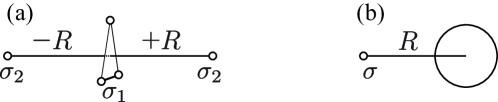
Figure 1: (a) Optimum 5$\alpha$ configuration that maximizes the overlap with the Hartree-Fock ground state of ${}^{20}{\rm Ne}$. A small triangle of 3$\alpha$ particles with radius $\sigma_{1}$ locates at the center and perpendicular to the longest axis of nucleus. Along this axis, two $\alpha$ particles with radius $\sigma_{2}$ are positioned at $\pm R$. (b) $\alpha$+${}^{16}{\rm O}$ configuration which also has large overlap with the Hartree-Fock ground state. $\alpha$ particle and Hartree-Fock ground state of ${}^{16}{\rm O}$ are placed with the distance $R$. This figure is reconstructed from Ref. [48]

Table 3: The overlap between the Hartree-Fock ground state of ${}^{20}{\rm Ne}$ and 5$\alpha$ Bloch-Brink wave function. The parameters of Bloch-Brink wave function are explained in the text and Fig. 1. This table is reconstructed from the data given in Ref. [48].

Skyrme	$\mathcal{O}_{BB}(\%)$	$R({\rm fm})$	$\sigma_{1}({\rm fm})$	$\sigma_{2}({\rm fm})$
SkI3	53	1.91	1.78	1.71
SkI4	49	1.86	1.78	1.71
Sly6	47	1.84	1.80	1.74
SkM*	36	1.59	1.77	1.73

The obtained Hartree-Fock ground state shows a strong prolate deformation. For this ground state, it was found that two different cluster configurations have large overlap. The first one is 5$\alpha$ configuration shown in the Fig. 1 (a). A small triangle of 3$\alpha$ particles with radius $\sigma_{1}$ locates at the center and perpendicular to the longest axis of nucleus. Along this axis, two $\alpha$ particles with radius $\sigma_{2}$ are positioned at $\pm R$. This configuration is consistent with the result reported in Ref. [51]. The optimal values of those parameters are listed in Tab. 3. The distance $R$ is around 1.9 fm and two $\alpha$ particles are well separated from the triangle implying non-negligible $\alpha$ correlation in the ground state, but it is not as large as that of ${}^{8}{\rm Be}$. The maximum value of the overlap is around 50% and much less than the case of ${}^{8}{\rm Be}$. Those results indicate the reduction of the cluster correlation compared to ${}^{8}{\rm Be}$ and increased importance of the cluster distortion effect due to the spin-orbit interaction and the formation of mean field.

Another configuration shown in Fig. 1 (b) also has large overlap and is more suggestive. In this configuration, $\alpha$ particle and Hartree-Fock wave function of ${}^{16}{\rm O}$ are placed with the distance $R$ and projected to the positive parity,

$$\Phi_{BB}(R)=n_{0}\mathcal{A}^{\prime}\left\{\psi_{\alpha}\Bigl{(}-\frac{4}{5}\bm{R}\Bigr{)}\psi_{{}^{16}{\rm O}}\Bigl{(}\frac{1}{5}\bm{R}\Bigr{)}\right\},\quad\bm{R}=(0,0,R),$$ (12)

$$\Phi_{BB}^{+}(R)=\frac{1+P_{x}}{2}\Phi_{BB}(R),$$ (13)

where $P_{x}$ denotes parity operator. The size of $\alpha$ particle and inter cluster distance $R$ are again optimized to maximize the overlap between $\Phi_{BB}^{+}(R)$ and Hartree-Fock ground state, as listed in Tab. 4.

Table 4: The overlap between the Hartree-Fock ground state of ${}^{20}{\rm Ne}$ and $\alpha$+${}^{16}{\rm O}$ Bloch-Brink wave function projected to positive parity. This table is reconstructed from the data given in Ref. [48].

	Bloch-Brink				GCM
Skyrme	$\mathcal{O}_{BB}(\%)$	$R({\rm fm})$	$\sigma({\rm fm})$		$\mathcal{O}_{GCM}(\%)$	$\sigma({\rm fm})$
SkI3	52	2.7	1.59		54	1.56
SkI4	48	2.5	1.62		49	1.52
Sly6	48	2.6	1.66		49	1.55
SkM*	36	2.4	1.64		36	1.53

It is interesting to note that this configuration has almost the same overlap with the 5$\alpha$ configuration. Furthermore, in this case, the size of $\alpha$ particle is close to that of free $\alpha$ particle and the inter-cluster distance is comparable with that of ${}^{8}{\rm Be}$. As we show later, the inter-cluster distance further increases when the angular momentum projection is performed. If we allow superposition of the Bloch-Brink wave functions, the overlap slightly increases.

Those results suggest that the ground state of ${}^{20}{\rm Ne}$ can be written in the following form,

$$\Phi(0^{+}_{1})=\sum_{N=N_{0}}^{\infty}e_{N}n_{N}\mathcal{A}\Set{\mathcal{R}_{N00}(\bm{r})\phi_{\alpha}\phi_{{}^{16}{\rm O}}}+\Phi_{\perp},\quad N_{0}=8$$ (14)

Here $n_{N}\mathcal{A}\Set{\mathcal{R}_{N00}(\bm{r})\phi_{\alpha}\phi_{{}^{16}{\rm O}}}$ is a normalized cluster model wave function in which the inter-cluster motion is described by the harmonic oscillator wave function $\mathcal{R}_{N00}(\bm{r})$, and $\Phi_{\perp}$ is non-cluster wave function that is orthogonal to $\mathcal{A}\Set{\mathcal{R}_{N00}(\bm{r})\phi_{\alpha}\phi_{{}^{16}{\rm O}}}$. From Tab. 4, the sum of the squared coefficient of superposition and the norm of $\Phi_{\perp}$ should be around 0.5,

$$\sum_{N=N_{0}}^{\infty}|e_{N}|^{2}\simeq 0.5,\quad\braket{\Phi_{\perp}}{\Phi_{\perp}}\simeq 0.5.$$ (15)

By a similar consideration to the case of ${}^{8}{\rm Be}$ and ${}^{16}{\rm O}$, we regard that the degrees-of-freedom of cluster excitation is embedded in the ground state of ${}^{20}{\rm Ne}$. If the inter-cluster motion $\mathcal{R}_{Nlm}(\bm{r})$ is excited, it will populates pronounced $\alpha$+${}^{16}{\rm O}$ cluster states.

Dual character of shell and cluster

Here, we summarize the insights obtained by the cluster analysis of the Hartree-Fock ground states.

1. All of nuclei examined here, ${}^{8}{\rm Be}$, ${}^{16}{\rm O}$ and ${}^{20}{\rm Ne}$, have large overlap with Bloch-Brink wave functions. This does not necessarily mean the prominent clustering, because at the limit of $R\rightarrow 0$, the cluster wave function becomes identical to the shell model wave function (Bayman-Bohr theorem).

2. However, the large overlap means that the ground state has the dual character of shell and cluster. Namely, the ground state wave function can be rewritten as a sum of cluster and non-cluster wave functions,

   $$\Phi(0^{+}_{1})=\sum_{N=N_{0}}^{\infty}e_{N}n_{N}\mathcal{A}\Set{\mathcal{R}_{N00}(\bm{r})\phi_{C_{1}}\phi_{C_{2}}}+\Phi_{\perp}.$$ (16)

   This expression implies that the degrees-of-freedom of cluster excitation is embedded in the ground state. If the inter-cluster motion $\mathcal{R}_{N00}(\bm{r})$ is excited, it yields excited states with pronounced clustering.

3. ${}^{8}{\rm Be}$ has large overlap with Bloch-Brink wave function. Therefore, the norm of $\Phi_{\perp}$ in Eq. (16) is rather small. Furthermore, because the inter-cluster distance is very large, the wave function with large principal quantum number $N$ is coherently superposed.

4. ${}^{16}{\rm O}$ has almost 100% overlap with Bloch-Brink wave function, and hence, $\Phi_{\perp}$ is negligible. Because the inter-cluster distance $R$ is very close to 0, the wave function with principal quantum number $N_{0}=4$ dominates.

5. ${}^{20}{\rm Ne}$ has approximately 50% overlap with Bloch-Brink wave function, and hence, the norm of $\Phi_{\perp}$ is approximately 0.5. The optimum inter-cluster distance $R$ is not small which means the moderate clustering in the ground state. In other words, $e_{N}$ for larger values of $N>N_{0}=8$ are not negligible.

Isoscalar monopole, dipole transitions and cluster states

In the previous section, we have seen that the Hartree-Fock ground states of ${}^{8}{\rm Be}$, ${}^{16}{\rm O}$ and ${}^{20}{\rm Ne}$ have large overlap with the cluster model (Bloch-Brink) wave functions and discussed that the ground states has dual character of shell and cluster. This fact implies that both of the single-particle and cluster excitations possibly occur, and if the inter-cluster motion is excited, prominent cluster states will be generated.

Here, by using ${}^{20}{\rm Ne}$ as an example, we show that the IS monopole and dipole transitions indeed induce the inter-cluster excitation to generate prominent cluster states. I first explain the nodal and angular excited cluster states of ${}^{20}{\rm Ne}$, and derive the analytical formula for transition matrix. It is shown that the transition matrices from the ground state to those exited cluster states are as large as Weisskopf estimates even if the ground state is not cluster state but a pure shell model state. Hence, the IS monopole and dipole excitations are regarded as good probe for cluster states.

Using Bloch-Brink wave function, I also show that the transition matrix is more enhanced, if the ground state has cluster structure. More realistic calculation by using antisymmetrized molecular dynamics (AMD) is also presented.

Nodal and angular excited cluster states

The ground state of ${}^{20}{\rm Ne}$ is written as,

$$\Phi(0^{+}_{1})=\sum_{N=N_{0}}^{\infty}e_{N}n_{N}\mathcal{A}\Set{\mathcal{R}_{N00}(\bm{r})\phi_{\alpha}\phi_{{}^{16}{\rm O}}}+\Phi_{\perp}.$$ (17)

As already discussed, this expression of the ground state wave function implies that the degrees-of-freedom of cluster excitation is embedded in the ground state, and the prominent cluster states are generated by the excitation of the inter-cluster motion.

The $\alpha$+${}^{16}{\rm O}$ cluster states in ${}^{20}{\rm Ne}$ have been studied in detail and are established well [52, 53, 54, 55, 56, 57, 58, 59]. Therefore, we already know the corresponding excited states which are populated by the excitation of inter-cluster motion. For example, if the nodal quantum number $n$ is increased, it yields the excited $0^{+}$ state described as,

$$\Phi(0^{+})=\sum_{N=N_{0}+2}^{\infty}f_{N}n_{N}\mathcal{A}^{\prime}\Set{\mathcal{R}_{N00}(\bm{r})\phi_{\alpha}\phi_{{}^{16}{\rm O}}}.$$ (18)

Here, the principal quantum number $N$ is equal to or larger than $N_{0}+2$, because of the relation $N=2n+l$. The $0^{+}_{4}$ state of ²⁰Ne observed as a broad resonance around 8.7 MeV has large $\alpha$ width comparable with Wigner limit and is attributed to this class of nodal excited cluster state.

Besides the nodal excitation, the angular excitation of the inter-cluster motion is also possible. For example, the angular excitation with $\Delta l=1$ (combined with the nodal excitation) yields the $1^{-}$ state,

$$\Phi(1^{-})=\sum_{N=N_{0}+1}^{\infty}g_{n}n_{N}\mathcal{A}^{\prime}\Set{\mathcal{R}_{N10}(r)\phi_{\alpha}\phi_{{}^{16}{\rm O}}},$$ (19)

where the principal quantum number $N$ is equal to or larger than $N_{0}+1$ because the angular momentum of the inter-cluster motion is increased to $l=1$. The $1^{-}_{1}$ state observed at 5.8 MeV also has large $\alpha$ width and is attributed to this class of angular excited cluster state. The cluster system with parity asymmetric intrinsic structure must have negative-parity states as well as positive-parity states. Therefore, this $1^{-}_{1}$ state is very important as the evidence for the asymmetric cluster structure of $\alpha$+${}^{16}{\rm O}$ [13].

Analytical expressions for transition matrix

Using the wave functions given in Eqs. (18) and (19), we discuss an analytic expression for the IS monopole and dipole transitions from the ground state to the nodal and angular excited cluster states. The IS monopole and dipole operators $\mathcal{M}^{IS0},\mathcal{M}_{\mu}^{IS1}$, their transition probabilities $B(IS0),B(IS1)$ and reduced matrix elements $M^{IS0},M^{IS1}$ are

$$\mathcal{M}^{IS0}=\sum_{i=1}^{A}(\bm{r}_{i}-\bm{r}_{\rm cm})^{2},$$ (20)

$$\mathcal{M}_{\mu}^{IS1}=\sum_{i=1}^{A}(\bm{r}_{i}-\bm{r}_{\rm cm})^{2}\mathcal{Y}_{1\mu}(\bm{r}_{i}-\bm{r}_{\rm cm}),$$ (21)

$$B(IS0;0^{+}_{1}\rightarrow 0^{+}_{4})=|M^{IS0}|^{2},\quad M^{IS0}=\braket{0^{+}_{4}}{\mathcal{M}^{IS0}}{0^{+}_{1}}=\braket{0^{+}_{4}}{\mathcal{M}^{IS0}}{0^{+}_{1}},$$ (22)

$$B(IS1;0^{+}_{1}\rightarrow 1^{-}_{1})=|M^{IS1}|^{2},\quad M^{IS1}=\braket{1^{-}_{1}}{\mathcal{M}^{IS1}}{0^{+}_{1}}=\sqrt{3}\braket{1^{-}_{1},J_{z}}{\mathcal{M}^{IS1}_{J_{z}}}{0^{+}_{1}},$$ (23)

where $\bm{r}_{i}$ denotes the $i$th nucleon coordinate, while $\bm{r}_{\rm cm}$ is the center-of-mass coordinate of the system. The solid spherical harmonics are defined as $\mathcal{Y}_{\lambda\mu}(\bm{r})\equiv r^{\lambda}Y_{\lambda\mu}(\hat{r})$.

To clarify the relationship between the monopole transition and clustering, we rewrite $\mathcal{M}_{\mu}^{IS0}$ in terms of the internal coordinates $\bm{\xi}_{i}$ of each cluster and the inter-cluster coordinate $\bm{r}$ defined as,

$$\bm{\xi}_{i}\equiv\left\{\begin{array}[]{l}\bm{r}_{i}-\bm{R}_{\alpha},\quad i\in\alpha\\ \bm{r}_{i}-\bm{R}_{{}^{16}{\rm O}},\quad i\in{}^{16}{\rm O},\\ \end{array}\right.\quad\bm{r}\equiv\bm{R}_{\alpha}-\bm{R}_{{}^{16}{\rm O}},$$ (26)

$$\bm{R}_{\alpha}\equiv\frac{1}{4}\sum_{i\in\alpha}\bm{r}_{i},\quad\bm{R}_{{}^{16}{\rm O}}\equiv\frac{1}{16}\sum_{i\in^{16}{\rm O}}\bm{r}_{i},$$ (27)

where the center-of-mass of $\alpha$ and ${}^{16}{\rm O}$ clusters $\bm{R}_{\alpha}$ and $\bm{R}_{{}^{16}{\rm O}}$ are introduced. With these coordinates, $\mathcal{M}_{\mu}^{IS0}$ is rewritten as follows,

$$\mathcal{M}_{\mu}^{IS0}= \sum_{i=1}^{A}(\bm{r}_{i}-\bm{r}_{\rm cm})^{2}=\sum_{i\in\alpha}\Bigl{(}\bm{\xi}_{i}+\frac{4}{5}\bm{r}\Bigr{)}^{2}+\sum_{i\in^{16}{\rm O}}\Bigl{(}\bm{\xi}_{i}-\frac{1}{5}\bm{r}\Bigr{)}^{2}$$

$$= \sum_{i\in\alpha}\xi_{i}^{2}+\sum_{i\in^{16}{\rm O}}\xi_{i}^{2}+\frac{16}{5}r^{2}$$ (28)

where the relations $\sum_{i\in\alpha}\bm{\xi}_{i}=\sum_{i\in^{16}{\rm O}}\bm{\xi}_{i}=0$ are used. This expression makes it clear that $\mathcal{M}^{\rm IS0}$ will populate nodal excited $0^{+}$ cluster states, because if operated to the ground state wave function given in Eq. (17), the last term will induce the nodal excitation of the inter-cluster motion. By a similar calculation, $\mathcal{M}^{IS1}_{\mu}$ is rewritten as follows (see Ref. [27] for the derivation),

$$\mathcal{M}^{IS1}_{\mu}= \sum_{i\in\alpha}\xi_{i}^{2}\mathcal{Y}_{1\mu}(\bm{\xi}_{i})+\sum_{i\in^{16}{\rm O}}\xi_{i}^{2}\mathcal{Y}_{1\mu}(\bm{\xi}_{i})$$

$$-\sqrt{\frac{32\pi}{9}}\Set{\frac{4}{5}\biggl{[}\sum_{i\in\alpha}\mathcal{Y}_{2}(\bm{\xi}_{i})\otimes\mathcal{Y}_{1}(\bm{r})\biggr{]}_{1\mu}-\frac{1}{5}\biggl{[}\sum_{i\in^{16}{\rm O}}\mathcal{Y}_{2}(\bm{\xi}_{i})\otimes\mathcal{Y}_{1}(\bm{r})\biggr{]}_{1\mu}}$$

$$+\left(\frac{4}{3}\sum_{i\in\alpha}\xi_{i}^{2}-\frac{1}{3}\sum_{i\in^{16}{\rm O}}\xi_{i}^{2}\right)\mathcal{Y}_{1\mu}(\bm{r})+\frac{48}{25}r^{2}\mathcal{Y}_{1\mu}(\bm{r}).$$ (29)

From this expression, we find that $\mathcal{M}_{\mu}^{IS1}$ will populate $1^{-}$ cluster states because the terms depending on $\mathcal{Y}_{1\mu}(\bm{r})$ and $r^{2}\mathcal{Y}_{1\mu}(\bm{r})$ in the second and third lines will induce the nodal and angular excitation of the inter-cluster motion.

If we assume that the ground state wave function is a pure shell model state, i.e. the wave function of the inter-cluster motion is the harmonic oscillator wave function with the lowest Pauli allowed principal quantum number $N_{0}$,

$$\Phi(0^{+}_{1})=n_{N_{0}}\mathcal{A}^{\prime}\Set{\mathcal{R}_{N_{0}00}(\bm{r})\phi_{\alpha}\phi_{{}^{16}{\rm O}}},$$ (30)

then, it is possible to calculate the transition matrix analytically. By substituting Eqs. (18), (19) and (30) into Eqs. (22) and (23), one gets

$$M^{IS0}= f_{N_{0}+2}\sqrt{\frac{\mu_{N_{0}}}{\mu_{N_{0}+2}}}\braket{R_{N_{0}0}}{r^{2}}{R_{N_{0}+20}}$$ (31)

$$M^{IS1}= \sqrt{\frac{3}{4\pi}}\Biggl{[}g_{N_{0}+1}\sqrt{\frac{\mu_{N_{0}}}{\mu_{N_{0}+1}}}\biggl{\{}\frac{16}{3}\left(\braket{r^{2}}_{\alpha}-\braket{r^{2}}_{{}^{16}{\rm O}}\right)\braket{R_{N_{0}0}}{r}{R_{N_{0}+11}}+\frac{48}{25}\braket{R_{N_{0}0}}{r^{3}}{R_{N_{0}+11}}\biggr{\}}$$

$$\qquad\qquad\qquad+\frac{3}{5}g_{N_{0}+3}\sqrt{\frac{\mu_{N_{0}}}{\mu_{N_{0}+3}}}\braket{R_{N_{0}0}}{r^{3}}{R_{N_{0}+31}}\Biggr{]},$$ (32)

where $\braket{r^{2}}_{\alpha}$ and $\braket{r^{2}}_{{}^{16}{\rm O}}$ are the mean-square radius of the clusters, and the matrix elements of harmonic oscillator are given as,

$$\braket{R_{N_{0}0}}{r^{2}}{R_{N_{0}+20}}=-\frac{\sigma^{\prime 2}}{2}\sqrt{(N_{0}+2)(N_{0}+3)},\quad\braket{R_{N_{0}0}}{r}{R_{N_{0}+11}}=\sigma^{\prime}\sqrt{\frac{N_{0}+3}{2}},$$

$$\braket{R_{N_{0}0}}{r^{3}}{R_{N_{0}+11}}=\sigma^{\prime 3}\frac{3N_{0}+5}{2}\sqrt{\frac{N_{0}+3}{2}},$$

$$\braket{R_{N_{0}0}}{r^{3}}{R_{N_{0}+31}}=-\sigma^{\prime 3}\frac{\sqrt{(N_{0}+2)(N_{0}+5)}}{2}\sqrt{\frac{N_{0}+3}{2}}.$$ (33)

And $\mu_{N}$ is so-called eigenvalue of RGM norm kernel defined as,

$$\mu_{N}=\braket{\mathcal{R}_{Nlm}(\bm{r})\phi_{\alpha}\phi_{{}^{16}{\rm O}}}{\mathcal{A}\set{\mathcal{R}_{Nlm}(\bm{r})\phi_{\alpha}\phi_{{}^{16}{\rm O}}}},$$ (34)

which is analytically calculable. Detailed explanations of above formula are given in Refs. [25, 27].

Table 5: List of the quantities used to evaluate Eq. (31) and (32). Radii of $\alpha$ and ¹⁶O clusters are calculated from the measured charge radii given in Ref. [60] and listed in the units of ${\rm fm}^{2}$. The oscillator parameters $\sigma$ and $\sigma^{\prime}$ are in units of fm. Coefficients $f_{N}$ and $g_{N}$ are obtained by the AMD calculation explained in the next section.

$N_{0}$	$\mu_{N_{0}}$	$\mu_{N_{0}+1}$	$\mu_{N_{0}+2}$	$\mu_{N_{0}+3}$	$\braket{r^{2}}_{\alpha}$	$\braket{r^{2}}_{{}^{16}{\rm O}}$
8	0.229	0.344	0.510	0.620	$(1.46)^{2}$	$(2.57)^{2}$
$\sigma$	$\sigma^{\prime}$	$g_{N_{0}+1}$	$f_{N_{0}+2}$	$g_{N_{0}+3}$
1.77	0.99	$\sqrt{0.39}$	$\sqrt{0.51}$	-$\sqrt{0.28}$

To evaluate the magnitude of transition matrices, we adopt the values listed in Table 5, where the values of $\sigma$, $\sigma^{\prime}$, $f_{N}$ and $g_{N}$ are taken from the AMD result explained later. Other variables are analytically calculable or taken from the experimental data. Assignment of those values to Eqs. (31) and (32) yields the estimate of IS monopole transition,

$$M^{IS0}=-7.67f_{10}=-5.48\ \rm fm^{2},$$ (35)

and IS dipole transition,

$$M^{IS1}=3.08g_{9}-7.36g_{11}=5.82\ \rm fm^{3}.$$ (36)

These results are compared with the single-particle estimates. Assuming the constant radial wave function as usual [61], Weisskopf estimates are given as

$$M_{\rm WU}^{IS0}=\frac{3}{5}(1.2A^{1/3})^{2}\simeq 0.864A^{2/3}\simeq 6.37\ \rm fm^{2},$$ (37)

$$M_{\rm WU}^{IS1}=\sqrt{\frac{3}{4\pi}}\frac{3}{6}(1.2A^{1/3})^{3}\simeq 0.422A\simeq 8.44\ \rm fm^{3},$$ (38)

which are slightly larger than but comparable with Eqs. (35) and (36).

Thus, the nodal and angular excited cluster states have strong IS monopole and dipole transitions from the ground state comparable with the Weisskopf estimate, even if the ground state is not a cluster state but an ideal shell model state. Since the single-particle transition is usually fragmented into many states, we expect that only the asymmetric cluster states can have strong transition strengths. Furthermore, as we will show below, the IS dipole strength is further amplified if the ground state has cluster structure.

Numerical estimate by using Bloch-Brink wave function

Here we show that the transition matrix $M^{IS1}$ is greatly amplified compared to the estimates made in the previous subsection, if the ground state has cluster correlation. I again employ Bloch-Brink wave function to discuss it,

$$\Phi_{BB}(R)=\frac{1+\pi P_{x}}{2}n_{0}\mathcal{A}^{\prime}\left\{\psi_{\alpha}\Bigl{(}-\frac{4}{5}\bm{R}\Bigr{)}\psi_{{}^{16}{\rm O}}\Bigl{(}\frac{1}{5}\bm{R}\Bigr{)}\right\},\quad\pi=\pm,\quad\bm{R}=(0,0,R),$$ (39)

and I project it to $0^{+}$ and $1^{-}$ states,

$$\Phi^{l\pi}_{BB}(R)=\frac{2l+1}{8\pi^{2}}\int d\Omega D^{l*}_{M0}(\Omega)R(\Omega)\Phi^{\pi}_{BB}(R).$$ (40)

Here $D^{l}_{MK}(\Omega)$ and $R(\Omega)$ denote Wigner $D$ function and rotation operator. By using this wave function, I calculated the transition matrix,

$$M^{IS1}(R_{0},R_{1})=\frac{\sqrt{3}\braket{\Phi_{\rm BB}^{1^{-}}(R_{1})}{\mathcal{M}^{IS1}_{0}}{\Phi_{\rm BB}^{0^{+}}(R_{0})}}{\sqrt{\braket{\Phi_{\rm BB}^{0^{+}}(R_{0})}{\Phi_{\rm BB}^{0^{+}}(R_{0})}\braket{\Phi_{\rm BB}^{1^{-}}(R_{1})}{\Phi_{\rm BB}^{1^{-}}(R_{1})}}}.$$ (41)

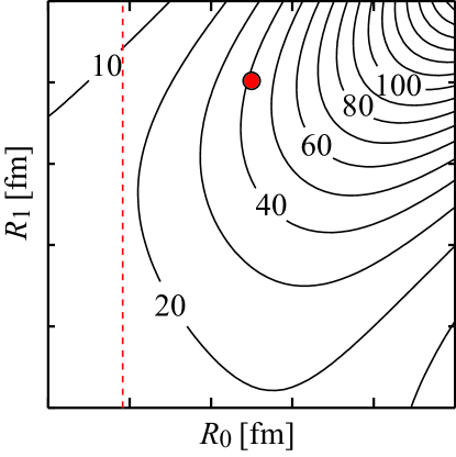
Figure 2: The transition matrix $M^{IS1}$ as function of the inter-cluster distances in the ground state ($R_{0}$) and in the $1^{-}$ state ($R_{1}$). The circle show the approximate position of the ground and the excited $1^{-}$ states obtained by AMD discussed in the next subsection. This figure is reconstructed from the data given in Ref. [27]

The calculated transition matrix $M^{IS1}$ is shown in Fig. 2 as function of the inter-cluster distances $R_{0}$ of the ground state and $R_{1}$ of the $1^{-}$ state. We can see that even for the small values of $R_{0}$ and $R_{1}$, $M^{IS1}$ is larger than the Weisskopf estimate. It is impressive that the matrix element is considerably amplified, as both of $R_{0}$ and $R_{1}$ growth.

By more detailed calculation explained in the next section, the position of the ground and $1^{-}$ states are estimated approximately at the circle in Fig. 2. Therefore, the transition strength is considerably amplified and regarded as a good probe for asymmetric clustering.

Realistic calculation with antisymmetrized molecular dynamics

I have discussed that the IS monopole and dipole transitions are greatly enhanced for the nodal and angular excited cluster states. However, in more realistic situation, there is the cluster distortion effect as expressed by Eq. (17). Therefore, for the quantitative discussion, we need more realistic calculation which takes cluster distortion effect into account. For this purpose, we introduce antisymmetrized molecular dynamics (AMD) which is a microscopic nuclear model able to describe both of cluster and non-cluster states. First, we briefly explain the framework of AMD. Readers are directed to Refs. [62, 63, 64] for more detail. Then, we discuss the numerical results obtained by AMD.

Framework of antisymmetrized molecular dynamics

In the present calculation, we employed the following microscopic $A$-body Hamiltonian,

$${H}=\sum_{i=1}^{A}{t}(i)+\sum_{i<j}^{A}{v}_{n}(ij)+\sum_{i<j}^{Z}{v}_{C}(ij)-{t}_{\rm cm},$$ (42)

where the Gogny D1S interaction [65] is used as an effective nucleon-nucleon interaction $v_{n}$. Coulomb interaction $v_{C}$ is approximated by a sum of seven Gaussians. The center-of-mass kinetic energy ${t}_{\rm cm}$ is exactly removed.

The intrinsic wave function of AMD is a Slater determinant of nucleon wave packets $\varphi_{i}$ represented by a localized Gaussian,

$$\Phi_{\rm int}={\mathcal{A}}\{\varphi_{1}\varphi_{2}...\varphi_{A}\},$$ (43)

$$\varphi_{i}({\bm{r}})=\exp\biggl{\{}-\sum_{\sigma=x,y,z}\nu_{\sigma}\Bigl{(}r_{\sigma}-\frac{Z_{i\sigma}}{\sqrt{\nu_{\sigma}}}\Bigr{)}^{2}\biggr{\}}\chi_{i}\xi_{i},$$ (44)

$$\chi_{i}=a_{i}\chi_{\uparrow}+b_{i}\chi_{\downarrow},\quad\xi_{i}={\rm proton}\ {\rm or}\ {\rm neutron},$$

where $\chi_{i}$ and $\xi_{i}$ represent spin and isospin wave functions. The intrinsic wave function is projected to the eigenstate of the parity,

$$\Phi^{\pi} =\frac{1+\pi P_{x}}{2}\Phi_{\rm int},\quad\pi=\pm.$$ (45)

Then, the parameters of the intrinsic wave function, ${\bm{Z}}_{i}$, $a_{i}$, $b_{i}$ and $\nu_{\sigma}$, are determined to minimize the expectation value of the Hamiltonian $\widetilde{E}$ that is defined as

$$\widetilde{E} =\frac{\langle\Phi^{\pi}|\hat{H}|\Phi^{\pi}\rangle}{\langle\Phi^{\pi}|\Phi^{\pi}\rangle}+V_{c},\quad V_{c}=v_{\beta}(\langle\beta\rangle-\beta)^{2}+v_{\gamma}(\langle\gamma\rangle-\gamma)^{2}.$$ (46)

Here the potential $V_{c}$ imposes the constraint on the quadrupole deformation of intrinsic wave function parameterized by $\braket{\beta}$ and $\braket{\gamma}$ [66]. The values of $v_{\beta}$ and $v_{\gamma}$ are chosen large enough so that $\braket{\beta},\braket{\gamma}$ are, after the energy minimization, equal to $\beta,\gamma$. By the energy minimization, we obtain the optimized wave function denoted by $\Phi^{\pi}_{\rm int}(\beta,\gamma)$ for given values of $(\beta,\gamma)$.

After the energy minimization, we project out an eigenstate of angular momentum,

$$\Phi^{J\pi}_{MK}(\beta,\gamma)=\frac{2J+1}{8\pi^{2}}\int d\Omega D^{J*}_{MK}(\Omega)\hat{R}(\Omega)\Phi^{\pi}(\beta,\gamma).$$ (47)

Then the wave functions with different values of quadrupole deformations $\beta$ and $\gamma$ are superposed.

$$\Psi^{J\pi}_{Mp}=\sum_{Ki}g_{Kip}\Phi^{J\pi}_{MK}(\beta_{i},\gamma_{i}),$$ (48)

and the coefficient of superposition $g_{Kip}$ and the eigenenergy $E^{J\pi}_{p}$ are determined by solving the Griffin-Hill-Wheeler equation [67, 68],

$$\sum_{i^{\prime}K^{\prime}}{H^{J\pi}_{KiK^{\prime}i^{\prime}}g_{K^{\prime}i^{\prime}p}}=E^{J\pi}_{p}\sum_{i^{\prime}K^{\prime}}{N^{J\pi}_{KiK^{\prime}i^{\prime}}g_{K^{\prime}i^{\prime}p}},$$ (49)

$$H^{J\pi}_{KiK^{\prime}i^{\prime}}=\langle{\Phi^{J\pi}_{MKi}|\hat{H}|\Phi^{J\pi}_{MK^{\prime}i^{\prime}}}\rangle,\quad N^{J\pi}_{KiK^{\prime}i^{\prime}}=\langle{\Phi^{J\pi}_{MKi}|\Phi^{J\pi}_{MK^{\prime}i^{\prime}}}\rangle.$$ (50)

Using the wave function given in Eq. (48) the transition matrix element is calculated. It is noted that AMD is able to describe the distortion of clusters and the coupling between the cluster states and non-cluster states, because all nucleons are treated independently.

Cluster states in ${}^{\bf 20}{\bf Ne}$ and IS monopole and dipole transitions

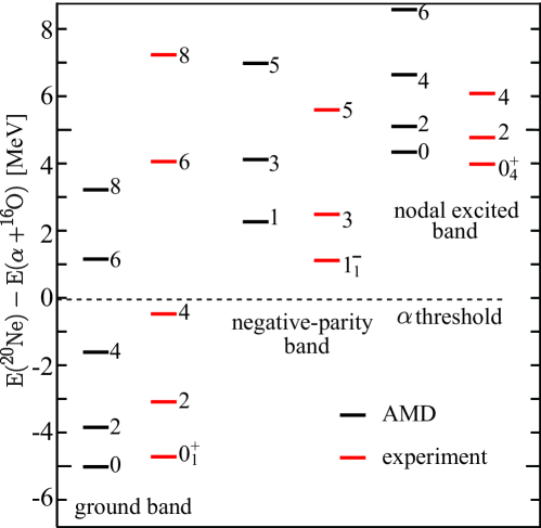
Figure 3: The observed and calculated $\alpha$+${}^{16}{\rm O}$ cluster states in ${}^{20}{\rm Ne}$ classified into three rotational bands. Energy is measured from the $\alpha$ threshold located at 4.7 MeV above the ground state.

The observed $\alpha$+${}^{16}{\rm O}$ cluster bands are summarized in Fig. 3 together with the result of AMD. The $0^{+}_{4}$ state at 8.7 MeV (4 MeV above the $\alpha$ threshold) is identified as the nodal excited state described by the wave function given in Eq. (18). A rotational band is built on this state. The $1^{-}_{1}$ state at 5.8 MeV (1.1 MeV above the $\alpha$ threshold) is the angular excited cluster state described by the wave function of Eq. (19). This $1^{-}_{1}$ state is very important because it is regarded as the evidence for the asymmetric clustering with $\alpha$+${}^{16}{\rm O}$ configuration.

Now, we examine the result of AMD. I calculated the amount of the cluster component defined by Eq. (6) and (8) in each states, and identified the states with large overlap as the $\alpha$+${}^{16}{\rm O}$ cluster states. Those cluster states are shown in Fig. 3 which reasonably agree with the observed spectrum. It is noted that AMD calculation also reproduces non-cluster states which are not shown in Fig. 3 and readers are directed to Ref. [63] for detailed discussions. Here, we focus on the ground $0^{+}_{1}$, the nodal excited $0^{+}_{4}$ and the angular excited $1^{-}_{1}$ states, whose properties are listed in Tab. 6.

Table 6: The properties of the ground, $0^{+}_{4}$ and $1^{-}_{1}$ states obtained by AMD. The overlap with the Bloch-Brink wave functions are given in percentage and the estimated inter-cluster distance is in units of fm. $M^{IS0}$ and $M^{IS1}$ are the IS monopole and dipole transition matrix from the ground state to the $0^{+}_{4}$ and $1^{-}_{1}$ states given in units of $\rm fm^{2}$ and $\rm fm^{3}$, respectively.

$0^{+}_{1}$				$0^{+}_{4}$				$1^{-}_{1}$
$\mathcal{O}_{BB}$	$R$	$\mathcal{O}_{GCM}$		$\mathcal{O}_{BB}$	$R$	$\mathcal{O}_{GCM}$		$\mathcal{O}_{BB}$	$R$	$\mathcal{O}_{GCM}$	$M^{IS0}$	$M^{IS1}$
54	3.5	60		58	6.5	69		81	5.0	88	12.2	34.4

The overlap between the ground state and the Bloch-Brink wave function amounts to approximately 50 to 60% which qualitatively consistent with the Hartree-Fock results discussed in the previous section. The estimated inter-cluster distance is 3.5 fm which is larger than that of Hartree-Fock result. This owes to the angular momentum projection which lowers energy of the deformed configuration and induces larger deformation of the ground state. The $0^{+}_{4}$ and $1^{-}_{1}$ states have larger overlap with the Bloch-Brink wave function and the larger inter-cluster distances than the ground state. This is apparently due to the excitation of the inter-cluster motion, which enlarges the inter-cluster distance and reduces the cluster distortion.

The calculated IS monopole and dipole transition matrix from the ground state to the $0^{+}_{4}$ and $1^{-}_{1}$ states are also listed in Tab. 6. It is evident that those excited cluster states have large transition matrix that are a few times larger than the Weisskopf estimates. This result suggests that both of the positive- and negative-parity cluster states can be strongly generated by the IS monopole and dipole transitions which will be good signature to identify the asymmetric clustering.

To summarize so far, I have discussed the dual character of shell and cluster, and IS monopole and dipole transitions which activate the degrees-of-freedom of cluster excitation. By the analysis of the Hartree-Fock wave functions, we have seen that the ground states of ${}^{8}{\rm Be}$, ${}^{16}{\rm O}$ and ${}^{20}{\rm Ne}$ have large overlap with Bloch-Brink wave functions. This fact means that the ground state has dual character of shell and cluster, and can be reasonably expressed by both of shell and cluster model wave functions. This dual character does not necessarily mean that the ground state has cluster structure, but means that the degrees-of-freedom of cluster excitation is embedded in the ground state. Therefore, both of the single-particle and cluster excitations are possible from the ground state.

As triggers to induce the cluster excitation, I have discussed IS monopole and dipole transitions of ${}^{20}{\rm Ne}$. I have shown that those operators bring about the nodal and angular excitations of the inter-cluster motion. By an analytic calculation, I have shown that the transition matrices from the ground state to the cluster states are comparable with the Weisskopf estimates, even if the ground state has an ideal shell structure. Furthermore, by using the Bloch-Brink wave function, it was shown that the IS dipole transition matrix is considerably amplified if the ground state has cluster structure. Finally, quantitative evaluation of the transition matrix was made by using AMD. As a result, it is confirmed that IS monopole and dipole transition matrices are sensitive to the cluster states. Therefore, it looks promising to search for unknown cluster states in heavier mass system such as ${}^{24}{\rm Mg}$ [69] and ${}^{28}{\rm Si}$ [70] by using IS monopole and dipole transitions as probe.

Linear-chains in neutron-rich carbon isotopes

In the study of neutron-rich nuclei, it was realized that the excess neutrons can induce or stabilize exotic cluster structure. The extreme but unstable 2$\alpha$ cluster structure of ${}^{8}{\rm Be}$ is stabilized by adding one or two neutrons (${}^{9}{\rm Be}$ and ${}^{10}{\rm Be}$ ). Furthermore, in more neutron-rich nuclei such as ${}^{11}{\rm Be}$ and ${}^{12}{\rm Be}$, the excess neutrons enhance 2$\alpha$ clustering and enlarge the inter-cluster distance. As a result, neutron-rich Be isotopes have a novel type of cluster structure in which the pronounced cluster core is surrounded and sustained by excess neutrons like a molecule [28, 29, 30, 31, 32, 33, 34, 35]. It was found a special class of neutron single-particle orbits called “molecular orbits” [28, 29, 30] is formed around the 2$\alpha$ cluster core, and play an essential role for stabilizing and inducing the clustering. Two kinds of molecular orbits so-called $\pi$- and $\sigma$-orbits shown in Fig. 4 are important. Roughly speaking, $\pi$-orbit plays a glue-like role and reduce the inter-cluster distance, while $\sigma$-orbit enhances the clustering and enlarges the inter-cluster distance. It was shown that the combinations of the excess neutrons occupying $\pi$- and $\sigma$-orbits reasonably explain the observed excitation spectra of Be isotopes.

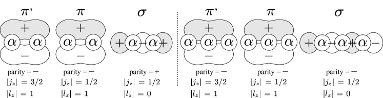
Figure 4: Left: molecular orbits in Be isotopes that have 2$\alpha$ cluster core. Right: An analogy of molecular orbits in 3$\alpha$ systems

This finding initiated the search for the linear-chain state of neutron-rich Carbon isotopes which is composed of linearly aligned three $\alpha$ particles with surrounding neutrons [34, 35, 36]. The linear-chain configuration of 3$\alpha$ particle was originally suggested by Morinaga [71] to explain the structure of the Hoyle state of ${}^{12}{\rm C}$. Later it was found that the Hoyle state is not a linear-chain state, but a dilute gas-like 3$\alpha$ cluster state. Nowadays, it is believed that the linear-chain structure of 3$\alpha$ particles is unstable against the bending motion (a perturbation which deviates from the linear alignment of $\alpha$ particles). Therefore, an extra mechanism is needed to realize the linear chain configuration. One of the strong candidates is the addition of the valence neutrons occupying the molecular orbit. It was shown that if the neutrons occupy the so-called $\sigma$-orbit, a deformed configuration of the core with an elongated shape is favored. Eventually, it was shown that the linear-chain configuration having $\sigma^{2}\pi^{2}$ configuration is possibly stabilized in ${}^{16}{\rm C}$ [36]. Motivated by this results, there are many theoretical studies on linear-chain of Carbon isotopes [37, 38, 39, 40, 41]. One major contribution is the studies based on the Hartree-Fock calculations [37, 40]. As a result of early stage research, I introduce the work by Maruhn et al. [37], and the recent situation is covered by N. Itagaki. Another contribution is from AMD [38, 39, 41], and I introduce a recent application. In both cases, the valence neutron configuration and stability of the linear chain are main concern, and I focus on ${}^{16}{\rm C}$ in the following.

A Hartree-Fock study

In Ref. [37], Maruhn and his collaborators performed the Hartree-Fock calculations to investigate the valence neutron configuration and stability of linear chain of ${}^{16}{\rm C}$. For this purpose, they started the iterative energy minimization from the initial states that have an ideal linear-chain configurations, that are constructed as follows.

• Gaussian wave functions with spin and isospin saturated quartets are placed at z = 0 and $z=\pm d$ fm, to represent the linearly aligned 3$\alpha$ clusters. The inter-cluster distance $d=3$ fm and the size of $\alpha$ cluster $\sigma=1.8$ fm were chosen as the initial condition.

• Neutrons occupying the $\sigma$-orbit were represented by deformed Gaussians (3 times broader in the $z$-direction) multiplied by $z(z-d)(z+d)$ to describe the nodes of $\sigma$-orbit.

• Neutrons in $\pi$-orbit were built by similar deformed Gaussians but multiplied by $x\pm iy$. By changing the combination with the direction of spin, two different $\pi$-orbits denoted by $\pi^{\prime}$ and $\pi$ are introduced. The former has $j_{z}=\pm 3/2$ and the spin-orbit interaction acts attractive, while the latter has $j_{z}=\pm 1/2$ and the repulsive spin-orbit interaction.

• Another neutron orbit denoted by $\delta$-orbit was also introduced and described by the deformed Gaussian multiplied by $z(x\pm iy)$.

By combining those $\sigma,\pi^{\prime},\pi$ and $\delta$ orbits with 3$\alpha$ linear chain, they prepared initial states having various linear chain configurations. If a certain linear-chain configuration is (meta)stable, it stays in a linear-chain configuration during a certain period of the iteration and eventually decays into the ground state. On the other hand, if a linear-chain configuration is unstable, it will decay into other configurations quickly.

The obtained results were interesting and unexpected. They found that the four configurations denoted by $\pi^{\prime 2}\pi^{2}$, $\pi^{\prime 2}\delta^{2}$, $\pi^{\prime 2}\delta\pi$, and $\pi^{\prime 2}\sigma\pi$ are stable, but other configurations decays into non-cluster states or populate an additional new linear-chain configuration denoted by $\pi^{\prime 2}\delta\pi^{\prime\prime}$. The properties of those molecular orbits are summarized in Tab. 7.

Table 7: The parity, $|j_{z}|$ and number of nodes along $z$-axis $n_{z}$ of valence neutron orbits denoted by $\pi^{\prime},\pi,\delta$ and $\pi^{\prime\prime}$. This table is reconstructed from Ref. [37].

type	parity	$|j_{z}|$	$n_{z}$
$\pi^{\prime}$	$-$	3/2	0
$\pi$	$-$	1/2	0
$\sigma$	$-$	1/2	3
$\delta$	$+$	3/2	1
$\pi^{\prime\prime}$	$-$	1/2	0

Those quantum numbers for $\pi^{\prime},\pi$ and $\sigma$ orbits agree with those discussed in the cluster models, while the $\delta$ and $\pi^{\prime\prime}$ orbits have not been considered in the preceding studies. All of those linear chain configurations appeared approximately 15 to 20 MeV in excitation energies as listed in Tab. 8.

Table 8: Excitation energies of linear chain configurations of ${}^{16}{\rm C}$ obtained by different Skyrme force parameters. This table is taken from Ref. [37].

Force	$\pi^{\prime 2}\pi^{2}$	$\pi^{\prime 2}\delta^{2}$	$\pi^{\prime 2}\delta\pi$	$\pi^{\prime 2}\sigma\pi$	$\pi^{\prime 2}\delta\pi^{\prime\prime}$
SkI3	14.5	19.5	17.0	17.5	19.1
SkI4	15.7	19.9	17.6	18.0	19.7
Sly6	15.4	18.9	17.0	17.3	19.0
SkM*	16.4	17.5	16.9	17.0	19.7

The quadrupole deformation parameter $\beta$ of those meta-stable linear chains are listed in Tab. 9.

Table 9: Quadrupole deformation parameter $\beta$ of the ground state and linear chain configurations of ${}^{16}{\rm C}$ obtained by different Skyrme force parameters. This table is taken from Ref. [37].

Force	g.s.	$\pi^{\prime 2}\pi^{2}$	$\pi^{\prime 2}\delta^{2}$	$\pi^{\prime 2}\delta\pi$	$\pi^{\prime 2}\sigma\pi$	$\pi^{\prime 2}\delta\pi^{\prime\prime}$
SkI3	0.34	0.69	0.82	0.76	0.76	0.88
SkI4	0.33	0.68	0.80	0.75	0.74	0.86
Sly6	0.32	0.68	0.81	0.75	0.75	0.87
SkM*	0.28	0.66	0.79	0.73	0.73	0.85

From this table, we can confirm that all of those meta-stable configurations have very stretched structure comparable with the hyperdeformation in which the ratio of the longest and shortest axis of nucleus reaches to 3:1. The density distribution of $\pi^{\prime 2}\delta^{2}$ configuration is shown in Fig. 5 an an example.

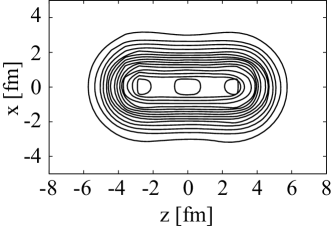
Figure 5: Total density distribution for the $\pi^{\prime 2}\delta^{2}$ configuration of ${}^{16}{\rm C}$. This figure is taken from Ref. [37].

They also analyzed the nucleon configurations. They classified nucleon single particle orbits into two groups; (1) the twelve orbits that constitute the 3$\alpha$ cluster core, and (2) the orbits of four valence neutrons. From the twelve orbits of (1) they reconstructed a Slater determinant corresponding to the 3$\alpha$ cluster core and made a cluster analysis which was already explained in the first part of this contribution. The results of analysis is given in Tab. 10.

Table 10: $\alpha$ cluster analysis of linear chain states of ${}^{16}{\rm C}$. The cluster wave function is composed of 3$\alpha$ particles with radius $\sigma$ positioned at $z=0,\pm R$. This result is obtained by the SkI3 parameter set. The data is taken from Ref. [37].

	$\pi^{\prime 2}\pi^{2}$	$\pi^{\prime 2}\delta^{2}$	$\pi^{\prime 2}\delta\pi$	$\pi^{\prime 2}\sigma\pi$	$\pi^{\prime 2}\delta\pi^{\prime\prime}$
$\mathcal{O}_{BB}(\%)$	63	65	64	64	66
$R$	2.44	2.68	2.56	2.56	2.80
$\sigma$	1.70	1.67	1.68	1.68	1.68

Compared to the result of ${}^{8}{\rm Be}$ given in Tab. 1, it is very interesting to see that the size of $\alpha$ particles is close to those of free $\alpha$ particles and in ${}^{8}{\rm Be}$. Furthermore, the inter-cluster distance is comparable or even larger than the ${}^{8}{\rm Be}$. From this table, we can conjecture that the $\pi$, $\pi^{\prime}$ orbits tend to reduce the inter-cluster distance, while the $\sigma$ and $\delta$ orbits enlarge it.

Thus, the Hartree-Fock calculation showed the possible existence of the linear-chain states in ${}^{16}{\rm C}$. It is surprising that the 3$\alpha$ cluster core having large overlap with cluster wave function was obtained without a priori assumption. The results of Hartree-Fock analysis may be summarized as follows.

1. Five different kinds of linear chain configurations are concluded as meta-stable local minimum state. All of those states appear around 15 to 20 MeV in excitation energies, which are much smaller than those predicted by the cluster model.

2. All of those states have 3$\alpha$ cluster cores which have large overlap with 3$\alpha$ Bloch-Brink wave function with linear configuration, whose parameters are close to those of ${}^{8}{\rm Be}$. This result confirms the formation of 3$\alpha$ core with linear configuration.

3. In addition to the $\pi^{\prime},\pi$ and $\sigma$ orbits, $\delta$ and $\pi^{\prime\prime}$ orbits are found, and they possibly stabilize the linear chain. On the other hand, the $\sigma^{2}\pi^{\prime 2}$ configuration which was suggested as the most stable configuration against the bending motion [36] was not obtained.

An AMD study

In addition to the Hartree-Fock analysis, several studies based on antisymmetrized molecular dynamics have also been performed. Here I introduce a resent result on ${}^{16}{\rm C}$ given in Ref. [39]. In this study, an AMD calculation was performed to search for the linear-chain state in ${}^{16}{\rm C}$. Advantages of the AMD calculation are in the projections of $J^{\pi}$, and the generator coordinate method. By $J^{\pi}$ projection, the rotational energy is subtracted and we can obtain more precise excitation energy. The GCM takes care of the orthogonality condition of the linear-chain states to other states having smaller excitation energies, which potentially increases the stability of the linear chain state. However, because the single particle wave packets are limited to the Gaussian form, the description of the molecular orbits is not as good as that of Hartree-Fock. Keeping those points in mind, we refer to the AMD results.

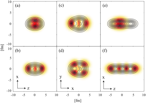
Figure 6: The density distribution of the ground (a)(b), triangular (c)(d) and linear-chain (e)(f) configurations. The contour lines show the proton density distributions and are common to the upper and lower panels. The color plots show the valence neutron orbits. The lower panels show the most weakly bound two neutrons, while the upper panel show the other two valence neutrons. This figure is taken from Ref. [27].

We first performed the constraint energy minimization to search for the strongly deformed minima. As a result, we obtained the global energy minimum corresponding to the ground state and two local minima which have cluster structure. The density distributions of the core (${}^{12}{\rm C}$) and those of four valence neutrons are shown in Fig. 6, and the properties of valence neutron orbits are listed in Tab. 11.

Table 11: The properties of valence neutron orbits shown in Fig. 6 which are occupied by two neutrons. Each column show the single particle energy $\varepsilon$ in MeV, the amount of the positive-parity component $p^{+}$ and the angular momenta. This table is taken from Ref. [27]

orbit	$\varepsilon$	$p^{+}$	$j$	$|j_{z}|$	$l$	$|l_{z}|$
(a)	$-8.24$	0.00	0.75	0.51	1.05	0.97
(b)	$-5.23$	0.99	2.21	0.51	1.80	0.38
(c)	$-5.74$	0.99	2.31	1.96	1.93	1.63
(d)	$-3.29$	0.98	2.33	1.88	2.07	1.83
(e)	$-5.32$	0.13	2.09	1.49	1.72	0.99
(f)	$-4.18$	0.03	2.89	0.53	2.72	0.18

As seen in its proton and valence neutron density distribution shown in Fig.6 (a) and (b), the ground state has no pronounced clustering. Four valence neutrons have an approximate $(0p_{1/2})^{2}(0d_{5/2})^{2}$ configuration that is confirmed from the properties of neutron single particle orbits listed in Tab. 11. The deviation from the spherical $p_{1/2}$ and $d_{5/2}$ orbits is due to prolate deformation of this state. As deformation increases, valence neutron configuration is changed and induces 3$\alpha$ clustering. A triaxially deformed 3$\alpha$ cluster configuration shown in Fig. 6 (c) and (d) appears. This configuration has 3$\alpha$ cluster core of an approximate isosceles triangular configuration with 3.2 fm long sides and 2.3 fm short side surrounded by valence neutrons occupying an approximate $(0d_{5/2})^{4}$ configuration.

Further increase of nuclear deformation realizes the linear-chain structure shown in Fig. 6 (e) and (f). As clearly seen in its density distributions, a linearly aligned 3$\alpha$ cluster core is accompanied by four valence neutrons. The interpretation of this configuration is given by the molecular orbit picture. Namely, as confirmed from the properties listed in Tab. 11, the valence neutron orbits are in good accordance with the $\pi^{\prime}$ and $\sigma$ orbits found in the Hartree-Fock result, and hence understood as $(\sigma)^{2}(\pi^{\prime})^{2}$ configuration.

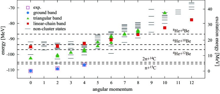
Figure 7: The calculated and observed positive-parity energy levels of ¹⁶C up to $J^{\pi}=12^{+}$ states. Open boxes show the observed states with the definite spin-parity assignments, and other symbols show the calculated result. This figure is taken from Ref. [27].

Figure 7 shows the spectrum obtained by the angular momentum projection and GCM calculation, where the obtained states are classified to the ’ground band’, ’triangular band’, ’linear-chain band’ and other non-cluster states by referring their cluster overlap. The member states of the ground band shown by circles are dominantly composed of the wave functions with $(sd)^{2}$ configuration. The calculated energy of the ground band is reasonably described. Owing to its triaxial deformed shape, the triangular configuration generates two rotational bands built on the $0^{+}_{2}$ and $2^{+}_{5}$ states. The member states have large overlap with the basis wave function shown in Fig. 6 (c)(d).

The linear-chain configuration appears as a rotational band built on the $0^{+}_{5}$ state at 15.5 MeV, that is close to the ⁴He+¹²Be and ⁶He+¹⁰Be threshold energies. The band head state $0^{+}_{5}$ has the largest overlap with the basis wave function shown in Fig.6 (e)(f). The moment-of-inertia is estimated as $\hbar/2\Im=112$ keV. Naturally, as the angular momentum increases, the excitation energy of the linear-chain state is lowered relative to other structures, and the $J^{\pi}=10^{+}$ member state at $E_{x}=27.8$ MeV becomes the yrast state. Thus, we predict the stable linear-chain configuration with molecular-orbits whose band-head energy is around ⁴He+¹²Be and ⁶He+¹⁰Be thresholds.

One of the concerns about the linear-chain configuration is its stability against the bending motion, and we confirm it by investigating the response to $\gamma$ deformation.

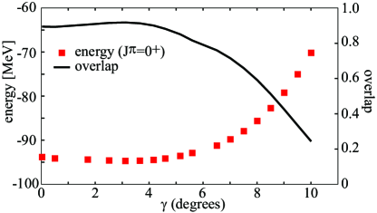
Figure 8: The boxes show the energy of the linear-chain configuration with $J^{\pi}=0^{+}$ as function of quadrupole deformation parameter $\gamma$. The solid line shows the overlap between the linear-chain state ($0^{+}_{5}$ state) and the basis wave functions. This figure is taken from Ref. [27]

Starting from the linear-chain configuration shown in Fig. 6 (e)(f), we gradually increased quadrupole deformation parameter $\gamma$ but kept $\beta$ constant to force the bending motion. Thus obtained curve shown in Fig. 8 by squares corresponds to the energy surface against the bending motion. It is almost constant for small value of $\gamma$, but rapidly increases for larger values of $\gamma$ indicating its stability. The solid line in Fig. 8 shows the overlap between the linear-chain $0^{+}_{5}$ state and the basis wave function shown by squares that is defined as,

$$O(\gamma)=|\langle\Psi(0^{+}_{5})|\Phi(0^{+};\gamma)\rangle|^{2}.$$ (51)

Here, $\Psi(0^{+}_{5})$ and $\Phi(0^{+};\gamma)$ denote the GCM wave function of the $0^{+}_{5}$ state and the linear chain configuration with bending motion. The overlap has its maximum at $\gamma=3.1$ degrees and falls off very quickly as $\gamma$ increases. Therefore the wave function of the linear-chain state is well confined within a region of small $\gamma$, and hence stable against the bending motion. We conjecture that this stability of linear-chain configuration originates in the orthogonality condition. Note that the energy of the linear-chain configuration is higher than that of the triangular configuration. Because the linear-chain state must be orthogonal to the triangular state, the bending motion is prevented by this orthogonality condition.

Thus, both of the Hartree-Fock and AMD calculations predict the existence of the linear-chain states of ${}^{16}{\rm C}$ around 15 MeV. However, as listed below, there are several disagreements between those models that require further investigations.

1. The favored valence neutron configurations are quite different. The Hartree-Fock suggested five meta-stable configurations, but none of them was found in AMD calculation. On the other hand, the cluster model and AMD suggest the stability of $(\pi^{\prime})^{2}(\sigma)^{2}$ configuration, which was turned out unstable in Hartree-Fock.

2. Nevertheless, the excitation energies of the linear chain in Hartree-Fock and AMD are similar to each other. There could be some universal rule that determines the excitation energy.

3. The discussion about the stability of the linear chain still remains rather simple estimations. The theoretical investigation of the $\alpha$ and neutron decay widths should be made. They are also important to identify the linear chain from the observed data.

Very recently, a couple of promising experimental data for linear chain configuration in for ${}^{14}{\rm C}$ [42, 45, 46, 47] and ${}^{16}{\rm C}$ [43, 44] were reported by several groups. We believe that further theoretical and experimental studies will reveal the linear chain in neutron-rich Carbon isotopes in near future.

Summary

In this contribution, I have discussed two topics. In the first part, the dual character of shell and cluster suggested by Bayman-Bohr theorem is discussed. The Hartree-Fock analysis was very helpful to understand the dual character. Owing to this dual character, both of the single-particle and cluster excitations (and of course as well as the collective excitations) are regarded as essential excitation modes of atomic nucleus. Indeed, by using ${}^{20}{\rm Ne}$ as an example, I’ve demonstrated that IS monopole and dipole transitions indeed induce the cluster excitation. Therefore, I expect that those transitions will be very powerful probe to search for the cluster states.

In the second half of the contribution, I discussed the linear-chain of the 3$\alpha$ particles in neutron-rich Carbon isotopes. Realization of such one dimensional structure is a long dream in nuclear physics, but found to be unrealistic in stable nucleus of ${}^{12}{\rm C}$. However, by the development in the physics of unstable nuclei, people realized that the valence neutrons may assist the cluster core to form the linear chain. Possible formation of such structure was investigated by Hartree-Fock and AMD. It was surprising that Hartree-Fock suggests various kind of linear chains, and both of Hartree-Fock and AMD predict similar excitation energies. However, there are several striking disagreements in their results, that must be resolved. With the help of the increasing experimental data, I believe that the linear chain states will be identified in near future.

References

- [1] G. Gamow, Constitution of Atomic Nuclei and Radioactivity, (Oxford University Press, 1931).
- [2] J. Chadwick, Nature 192, 312 (1932).
- [3] K. Wildermuth and Th. Kanellopoulos, Nucl. Phys. 7, 150 (1958).
- [4] K. Wildermuth and Th. Kanellopoulos, Nucl. Phys. 9, 449 (1958/59).
- [5] J. A. Wheeler, Phys. Rev. 52, 1083 (1937).
- [6] K. Wildermuth and Y. C. Tang, A Unified Theory of the Nucleus (Academic, New York, 1977).
- [7] D. M. Brink, Proc. Int. School of Physics Enrico Fermi, Course 36, Varenna, ed. C. Bloch (Academic Press, New York, 1966).
- [8] C. Beck (Ed.), Clusters in Nuclei Vol. 1, Lecture Notes in Physics, vol. 818, (Springer, Berlin, Heidelberg, 2010).
- [9] C. Beck (Ed.), Clusters in Nuclei Vol. 2, Lecture Notes in Physics, vol. 848, (Springer, Berlin, Heidelberg, 2012).
- [10] C. Beck (Ed.), Clusters in Nuclei Vol. 3, Lecture Notes in Physics, vol. 875, (Springer, Berlin, Heidelberg, 2014).
- [11] B. F. Bayman, and A. Bohr, Nucl. Phys. 9, 596 (1958/1959).
- [12] J. P. Elliott, Proc. R. Soc. London A 245, 562 (1958).
- [13] H. Horiuchi, and K. Ikeda, Prog. Theor. Phys. 40, 277 (1968).
- [14] E. Uegaki, S. Okabe, Y. Abe, and H. Tanaka, Prog. Theor. Phys. 57, 1262 (1977).
- [15] M. Kamimura, Nucl. Phys. A 351, 456 (1981).
- [16] P. Descouvemont, and D. Baye, Phys. Rev. C 36, 54 (1987).
- [17] Y. Kanada-En’yo, Phys. Rev. Lett. 81, 5291 (1998).
- [18] A. Tohsaki, H. Horiuchi, P. Schuck, and G. Röpke, Phys. Rev. Lett. 87, 192501 (2001).
- [19] T. Neff, and H. Feldmeier, Nucl. Phys. A 738, 357 (2004).
- [20] T. Yamada, H. Horiuchi, K. Ikeda, Y. Funaki and A. Tohsaki, Jour. of Phys. Conf. Ser. 111, 012008 (2008).
- [21] Y. Funaki, A. Tohsaki, H. Horiuchi, P. Schuck, and G. Röpke, Eur. Phys. J A 28, 259 (2006).
- [22] Y. Funaki, H. Horiuchi and A. Tohsaki, Prog. Part. Nucl. Phys. 82, 78 (2015).
- [23] Y. Suzuki, Nucl. Phys. A 470, 119 (1987).
- [24] Y. Suzuki, and S. Hara, Phys. Rev. C 39, 658 (1989).
- [25] T. Yamada, Y. Funaki, H. Horiuchi, K. Ikeda, and A. Tohsaki, Prog. Theor. Phys. 120, 1139 (2008).
- [26] H. Horiuchi, J. Phys. Conf. Ser. 569, 012001 (2014).
- [27] Y. Chiba, M. Kimura and Y. Taniguchi, Phys.Rev. C 93, 034319 (2016).
- [28] M. Seya, M. Kohno, and S. Nagata, Prog. Theor. Phys. 65, 204 (1981).
- [29] W. von Oertzen, Z. Phys. A 354, 37 (1996); ibid 357, 355 (1997).
- [30] N. Itagaki and S. Okabe, Phys. Rev. C 61, 044306 (2000).
- [31] P. Descouvemont, Nucl. Phys. A 699, 463 (2002).
- [32] Y. Kanada-En’yo, H. Horiuchi, and A. Ono, Phys. Rev. C 52, 628 (1995).
- [33] Y. Kanada-En’yo and H. Horiuchi, Phys. Rev. C 68, 014319 (2003).
- [34] W. von Oertzen, Z. Physik A 357, 355 (1997).
- [35] W. von Oertzena, M. Freer, and Y. Kanada-En’yo, Phys. Rep. 432, 43 (2006).
- [36] N. Itagaki, S. Okabe, K. Ikeda, and I. Tanihata, Phys. Rev. C 64, 014301 (2001).
- [37] J. A. Maruhn, N. Loebl, N. Itagaki, and M. Kimura, Nucl. Phys. A 833, 1 (2010).
- [38] T. Suhara, Y. Kanada-Enyo, Phys. Rev. C 84, 024328 (2011).
- [39] T. Baba, Y. Chiba, and M. Kimura, Phys. Rev. C 90, 064319 (2014).
- [40] P. W. Zhao, N. Itagaki, and J. Meng, Phys. Rev. Lett. 115 , 022501 (2015).
- [41] T. Baba, and M. Kimura, Phys. Rev. C 94, 044303 (2016).
- [42] M. Freer et al., Phys. Rev. C 90, 054324 (2014).
- [43] S. Koyama et al., private communication.
- [44] D. Dell’Aquila et al., Phys. Rev. C 93, 024611 (2016).
- [45] A. Frisch et al., Phys. Rev. C 93, 014321 (2016).
- [46] H. Yamaguchi et al., arXiv:1610.06296.
- [47] Z. Y. Tian et al., Chi. Phys. C 40, 111001 (2016).
- [48] J. A. Maruhn, M. Kimura, S. Schramm, P.-G. Reinhard, H. Horiuchi, and A. Tohsaki Phys. Rev. C 74, 044311 (2006).
- [49] R. B. Wiringa, S. C. Pieper, J. Carlson, and V. R. Pandharipande, Phys. Rev. C 62, 014001 (2000).
- [50] H. Horiuchi, Prog. Theor. Phys. Suppl. 62, 90 (1977).
- [51] J. Zhang, W. D. M. Rae, and A. C. Merchant, Nucl. Phys. A 575, 61 (1994).
- [52] T. Matsuse, M. Kamimura, and Y. Fukushima, Prog. Theor. Phys. 53, 706 (1975).
- [53] B. Buck, C. B. Dover, and J. -P. Vary, Phys. Rev. C 11, 1803 (1975).
- [54] P. -H. Heenen, Nucl. Phys. A 272, 399 (1976).
- [55] Y. Fujiwara, H. Horiuchi, and R. Tamagaki, Prog. Theor. Phys. 62, 122 (1979).
- [56] M. Kruglanski and D. Baye, Nucl. Phys. A 548, 39 (1992).
- [57] M. Dufour. P. Descouvemont, and D. Baye, Phys. Rev. C 50, 795 (1994).
- [58] B. Zhou, Y. Funaki, H. Horiuchi, Z. Ren, G. Röpke, P. Schuck, A. Tohsaki, C. Xu, and T. Yamada, Phys. Rev. Lett. 110, 262501 (2013).
- [59] E. F. Zhou, J. M. Yao, Z. P. Li, J. Meng, P. Ring, Phys. Lett. B, in print.
- [60] I. Angelia, and K. P. Marinovab, Atom. data and Nucl.Data Tables, 99, 69 (2013).
- [61] J. A. Maruhn and W. Greiner, Nuclear Models (Springer, 1996).
- [62] Y. Kanada-En’yo, M. Kimura and H. Horiuchi, C. R. Physique 4, 497 (2003).
- [63] M. Kimura Phys. Rev. C 69, 044319 (2004).
- [64] Y. Kanada-En’yo, M. Kimura and A. Ono, PTEP 2012, 01A202 (2012).
- [65] J. F. Berger, M. Girod, and D. Gogny, Comput. Phys. Comm. 63 (1991) 365.
- [66] M. Kimura, R. Yoshida, and M. Isaka, Prog. Theor. Phys. 127, 287 (2012).
- [67] D. L. Hill and J. A. Wheeler, Phys. Rev. 89, 112 (1953).
- [68] J. J. Griffin and J. A. Vfheeler, Phys. Rev. 108, 311 (1957).
- [69] T. Kawabata et al., Jour. Phys. Conf. Ser. 436, 012009 (2013).
- [70] M. Itoh et al., Phys. Rev. C 88, 064313 (2013).
- [71] H. Morinaga, Phys. Rev. 101, 254 (1956).