Contact-aware simulations of particulate Stokesian suspensions

Abstract

We present an efficient, accurate, and robust method for simulation of dense suspensions of deformable and rigid particles immersed in Stokesian fluid in two dimensions. We use a well-established boundary integral formulation for the problem as the foundation of our approach. This type of formulations, with a high-order spatial discretization and an implicit and adaptive time discretization, have been shown to be able to handle complex interactions between particles with high accuracy. Yet, for dense suspensions, very small time-steps or expensive implicit solves as well as a large number of discretization points are required to avoid non-physical contact and intersections between particles, leading to infinite forces and numerical instability.

Our method maintains the accuracy of previous methods at a significantly lower cost for dense suspensions. The key idea is to ensure interference-free configuration by introducing explicit contact constraints into the system. While such constraints are unnecessary in the formulation, in the discrete form of the problem, they make it possible to eliminate catastrophic loss of accuracy by preventing contact explicitly.

Introducing contact constraints results in a significant increase in stable time-step size for explicit time-stepping, and a reduction in the number of points adequate for stability.

1 Introduction

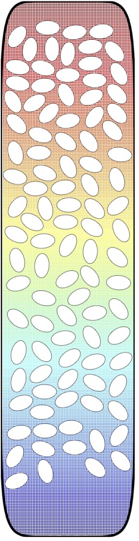
((a)) $t=0$

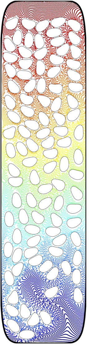
((b)) $t=1.2$

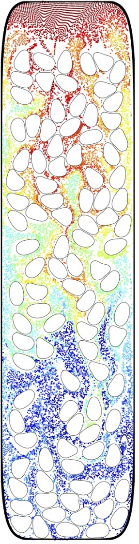
((c)) $t=5.0$

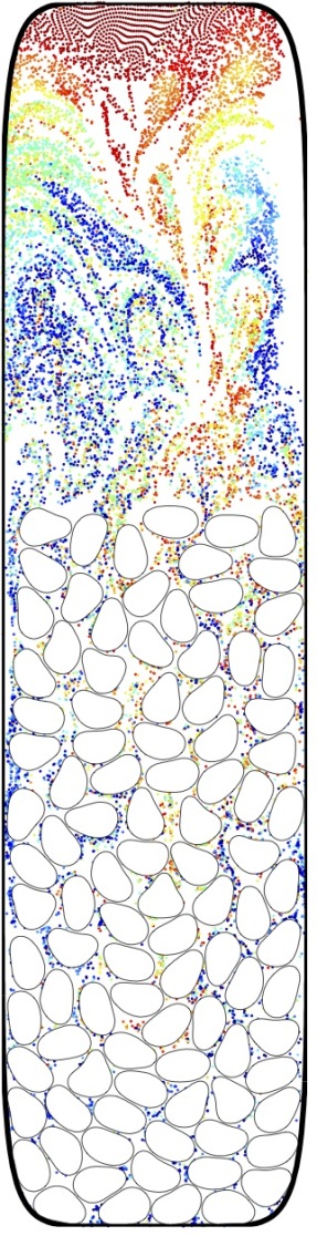
((d)) $t=30$

Figure 1: Sedimentation of one hundred vesicles. Vesicles are randomly placed in a container, where only gravitational force is present. LABEL:sub@sfg:sed-snap1 The initial configuration. The colored tracer particles are shown for visualization purposes and are not hydrodynamically active. LABEL:sub@sfg:sed-snap2 and LABEL:sub@sfg:sed-snap3 The intermediate states; we see that as vesicles move downward they induce a strong back flow. LABEL:sub@sfg:sed-snap4 shows the state where the simulation was terminated. As the vesicles accumulate at the bottom of the container, many collision areas stay active. Nonetheless, the vesicles are stacked stably and without any artifact from the collision handling.

Particulate Stokesian suspensions of deformable and rigid particles are prevalent in nature and have many important industrial applications, for example, emulsions, colloidal structures, particulate suspensions, and blood. Most of these examples are complex fluids, i.e., fluids with unusual macroscopic behavior, often defying a simple constitutive-law description. A major challenges in understanding the physics of complex fluids is the link between microscopic and macroscopic fluid behavior. Dynamic simulation is a powerful tool [33, 7] to gain insight into the underlying physical principles that govern these suspensions and to obtain relevant constitutive relationships.

Nevertheless, simulating dense suspensions of rigid and deformable particles entails many numerical challenges, one of which is the numerical breakdown due to collision of particles, making robust treatment of contact vital for these simulations. To this end, we present an efficient, accurate, and robust method for simulation of dense suspensions in Stokesian fluid in 2d (e.g., Fig. 1), which is extendable to 3d. We use the boundary integral formulation to represent the flow and impose the contact-free condition as a constraint. This work focuses mainly on suspensions of rigid bodies and vesicles with high volume fractions, in which multiple particles are in contact or near-contact.

Vesicles are closed deformable membranes suspended in a viscous medium. The dynamic deformation of vesicles and their interaction with the Stokesian fluid play an important role in many biological phenomena. They are used to understand the properties of biomembranes [19, 32], and to simulate the motion of blood cells, in which vesicles with moderate viscosity contrast are used to model red blood cells and high viscosity contrast vesicles or rigid particles are used to model white blood cells [6].

Boundary integral formulations offers a natural approach for accurate simulation of vesicle flows, by reducing the problem to solving equations on surfaces, and eliminating the need for discretizing changing 3D volumes. However, in non-dilute suspensions, these methods are hindered by difficulties: inaccuracies in computing near-singular integrals, and artificial force singularities caused by (non-physical) intersection of particles. Contact situations in the Stokesian particulate flows occur frequently when the volume fraction of suspensions is high, viscosity contrast of vesicles is high, or rigid particles are present. The dynamics of particle collision in Stokes flow are governed by the lubrication film formation and drainage, which has a time scale much shorter than that of the flow [18]. Solely relying on the hydrodynamics to prevent contact requires the accurate solution of the flow in the lubrication film, which in turn entails very fine spatial and temporal resolution as well as expensive implicit time-stepping—imposing excessive computational burden as the volume fraction increases.

While adaptive time-stepping [47, 48] goes a long way in maintaining stability and efficiency in dilute suspensions, the time-step is determined by the closest pair of vesicles, and tends to be uniformly small for dense suspensions.

In this work we take a different approach: we augment the governing equations with the contact constraint. While from the point of view of the physics of the problem such a constraint is redundant, as non-penetration is ensured by fluid forces, in numerical context it plays an important role, improving both robustness and accuracy of simulations. Typically, a contact law/constraint is characterized by conditions of non-penetration, no-adhesion as well as a mechanical complementarity condition, i.e., the contact force is zero when there is no collision. These three conditions are known as Signorini conditions in the context of contact mechanics or KKT conditions in the context of constrained optimization [60, 35].

1.1 Our contributions

Contact constraints ensure that the discretized system remains intersection-free, even for relatively coarse spatial and temporal discretizations. The resulting problem is a Nonlinear Complementarity Problem (NCP), which we linearize and solve using an iterative method that avoids explicit construction of full matrices. We describe an implicit-explicit time-stepping scheme, adapting Spectral Deferred Correction (SDC) to our constrained setting, Section 3.2.

In our approach, the minimum distance between vesicles is controlled by constraints, and is independent of the temporal resolution. While this requires solving additional auxiliary equations for the constraint forces at every step, this additional cost is more than compensated by the ability of our method to maintain larger time-steps, and lower spatial resolutions for a given target error.

For high volume fraction, our method makes it possible to increase the step size by at least an order of magnitude, and the simulation remain stable even for relatively coarse spatial discretizations (16 points per vesicle, versus at least 64 needed for stability without contact resolution).

1.2 Synopsis of the method

We use the boundary integral formulation based on [58, 50, 47]; the basic formulation uses integral equation form of the problem and includes the effects of the viscosity contrast, fixed boundaries, as well as deformable and rigid moving bodies. We add contact constraints to this formulation, as an inequality constraint on a gap function that is based on space-time intersection volume [23]. The contact force is then parallel to the gradient of this volume with the Lagrange multiplier as its magnitude.

In case of multiple simultaneous contact, this leads to a Nonlinear complementarity problem (NCP) for the Lagrange multipliers, which we solve using a Newton-like matrix-free method, as a sequence of Linear Complementarity Problems (LCP) [9, 13], solved iteratively using GMRES. The spectral Fourier bases are used for spatial discretization. For time stepping, we use semi-implicit backward Euler or semi-implicit Spectral Deferred Correction (SDC).

1.3 Related work

Related work on Stokesian particle flows

Stokesian particle models are employed to theoretically and experimentally investigate the properties of biological membranes [53], drug-carrying capsules [56], and blood cells [36, 41]. There is an extensive body of work on numerical methods for Stokesian particulate flows and an excellent review of the literature up to 2001 can be found in [43]. Reviews of later advances can be found in [58, 50, 51]. Here, we briefly summarize the most important numerical methods and discuss the most recent developments.

Integral equation methods have been used extensively for the simulation of Stokesian particulate flows such as droplets and bubbles [52, 66, 30, 29], vesicles [41, 17, 58, 55, 50, 14, 63, 64, 51], and rigid particles [62, 39, 40]. Other methods—such as phase-field approach [8, 10], immersed boundary and front tracking methods [25, 61], and level set method [27]—are used by several authors for the simulation of particulate flows.

For certain flow regimes, near interaction and collision of particles has been a source of difficulty, which was addressed either by spatial and temporal refinement to resolve the correct dynamics (increasing the computational burden) or by the introduction of repulsion forces (making the time-stepping stiff).

[54] presented a framework for dynamic simulation of rigid particles with spherical or cylindrical shapes, in which the lubrication forces were included directly by putting Stokes doublets at the contact midpoint. The magnitude of lubrication force was computed using asymptotic analysis. To maintain the accuracy in the interaction of deformable drops, [68, 29, 67] resorted to time-step refinement where the time step is kept proportional to particle distance $d$. [68, 67] keep the time step proportional to $\sqrt{d}$. [29] adjust both the grid spacing around the contact region and the time-step to be proportional to $d$. [17] resorted to repulsion force to avoid contact in a 2d particulate flow. In a later work for 3d, [17] and coauthors [65] observed that significantly larger repulsion force density are needed in three dimensions, as the total repulsion force is distributed over a smaller region, when measured as a fraction of the total surface area/length. Consequently, they used a purely kinematic collision handing, in which, after each time-step, the intersecting points are moved outside.

[48] applies adaptive time-stepping and backtracking to resolve collisions. Similarly, [37] present an interesting integral equation method for the flow of droplets in two dimensions with a specialized quadrature scheme for accurate near-singular evaluation enabling simulation of flows with close to touching particles. While methods using adaptivity both in space and time are the most robust and accurate, they incur excessive cost as means of collision handling.

Related work on contact response

A broad range of methods were developed for collision detection and response. While the work in contact mechanics often focuses on capturing the physics of the contact correctly (e.g., taking into account friction effects), the work in computer graphics literature emphasizes robustness and efficiency. In our context, robustness and efficiency are particularly important, as we aim to model vesicle flows with high density and large numbers of particles. Physical correctness has a somewhat different meaning: as we know that if the forces and surfaces in the system are resolved with high accuracy, the contacts would not occur, our primary emphasis is on reducing the impact of the artificial forces associated with contacts on the system.

There is an extensive literature on contact handling in computational contact mechanics mainly in the context of FEM mechanical and thermal analysis [24, 59, 60, 16, 57, 46, 26]. [59, 60] presents in-depth reviews of the contact mechanics framework. The works in contact mechanics literature can be categorized based on their ability in handling large deformations and/or tangential friction. In some of the methods, to simplify the problem, small deformation assumption is used to predefine the active part of the boundary as well as to align the FEM mesh. Numerical methods for contact response can be categorized as (i) penalty forces, (ii) impulse/kinematic responses, and (iii) constraint solvers.

From algorithmic viewpoint, contact mechanics methods in FEM include: (i) Node-to-node methods where the contact between nodes is only considered. The FEM nodes of contacting bodies need to aligned and therefore this method is only applicable to small deformation. (ii) Node-to-surface methods check the collision between predefined set of nodes and segments. Similar to node-to-node methods, these methods can only handle small deformations. (iii) Surface-to-surface methods, where the contact constraint is imposed in weak form. In contrast to the two previous class of algorithms, methods in this class are capable of handling large deformations. Mortar Method is well-known within this class of algorithms [26, 16, 46, 57]. The Mortar Method was initially developed for connecting different non-matching meshes in the domain decomposition approaches for parallel computing, e.g., [45].

In these methods, no-penetration is either enforced as a constraint using a Lagrangian (identified with the contact pressure) or penalty force based on a gap function. To the best of our knowledge, for contact mechanics problems, a signed distance between geometric primitives is used as the gap function, in contrast to our approach where we use space-time interference volume.

[16] present a frictionless contact resolution framework for 2d finite deformation using Mortar Method using penalty force or Lagrange multiplier. [57] use similar method for frictional contact in 2d. [46] use Mortar Method for large deformation contact using quadratic element.

Our problem has similarities to large-deformation frictionless contact problems in contact mechanics. An important difference however, is the presence of fluid, which plays a major role in contact response.

Application of boundary integral methods in contact mechanics is rather limited compared to the FEM methods [12, 20]. [12] used Boundary Element Method for the static contact problem where Coulomb friction is presented. [20] solved static problem with load increment and contact constraint on displacement and traction.

In computer graphics literature, a set of commonly used and efficient methods are based on [44], a method for the collision handling of mass-spring cloth models. To ensure that the system remains intersection-free, zones of impact are introduced and rigid body motion is enforced in each zone of impact; while this method works well in practice, its effects on the physics of the objects are difficult to quantify.

Penalty methods are common due to the ease in their implementation, but suffer from time-stepping stiffness and/or the lack of robustness. [5] uses implicit time-stepping coupled with repulsion force equal to the variation of the quadratic constraint energy with respect to control vertices. Soft collisions are handled by the introduction of damped spring and rigid collisions are enforced by modification to the mass matrix. [15] introduced Layered Depth Images to allow efficient computation of the collision volumes and their gradients using GPUs. A penalty force proportional to the gradient is used to resolve collisions. However, the stiffness of the repulsion force varies greatly (from $10^{5}$ to $10^{10}$) in their experiments. To address these difficulties, [22] present a framework for robust simulation of contact mechanics using penalty forces through asynchronous time-stepping, albeit at a significant computational cost. Alternatively, one can view collision response as an instantaneous reaction (an impulse), i.e., an instantaneous adjustment of the velocities. However, such adjustments are often problematic in the case of multiple contacts, as these may lead to a cyclic “trembling” behavior.

Our method belongs to a large family of constraint-based methods, which are increasingly the standard approach to contact handling in graphics. This set of methods meets our goals of providing robustness and improving efficiency of contact response, while minimizing the impact on the physics of the system (as virtual forces associated with constraints do not do work).

[11] start from Signorini’s law and derive the contact force formulation. The resulting equation is an LCP that is solved by Gauss–Seidel like iterations, sequentially resolving contacts until reaching the contact free state. [21] focus on robust treatment of collision without simulation artifacts. To enforce the no-collision constraint, this work uses an impulse response that gives rise to an LCP problem for its magnitude. To reduce the computational cost, the LCP solution (the Lagrange multiplier) is approximated by solving a linear system. [38] uses a linear approximation to contact constraints and a semi-implicit discretization, solving a mixed LCP problem at each iteration.

Our approach is directly based on [23] and is closest to [2], in which the intersection volume and its gradient with respect to control vertices are computed at the candidate step. The non-collision is enforced as a constraint on this volume, which lead to a much smaller system compared to distance formulation between geometric primitives. The constrained formulation leads to an LCP problem. [23] assumes linear trajectory between edits and define space-time interference volume and uses it as a gap function and we use similar formulation to define the interference volume.

1.4 Nomenclature

In Section 1.4 we list symbols and operators frequently used in this paper. Throughout this paper, lower case letters refer to scalars, and lowercase bold letters refer to vectors. Discretized quantities are denoted by sans serif letters.

Symbol	Definition
$\gamma_{i}$	The boundary of the i vesicle
$\gamma$	$\cup_{i}\gamma_{i}$
$\nu_{i}$	The viscosity contrast
$\mu$	Viscosity of the ambient fluid
$\mu_{i}$	Viscosity of the fluid inside i vesicle
$\sigma$	Tension
$\chi$	Shear rate
$\varpi_{i}$	The domain enclosed by $\gamma_{i}$
$\varpi$	$\cup_{i}\varpi_{i}$
$d$	Separation distance of particles
$d_{m}$	Minimum separation distance
$\bm{f}_{\sigma}$	Tensile force
$\bm{f}_{b}$	Bending force
$\bm{f}_{c}$	Collision force
$h$	Distance between two discretization points (on each surface)

Symbol	Definition
$J$	Jacobian of contact volumes $V$
$\bm{n}$	Unit outward normal
$\bm{u}$	Velocity
$\bm{u}^{\infty}$	The background velocity field
$V$	Contact volumes
$\bm{X}$	Coordinate of a (Lagrangian) point on a surface
$\mathcal{G}$	Stokes Single-layer operator
$\mathcal{T}$	Stokes Double-layer operator
LCP	Linear Complementarity problem
NCP	Nonlinear Complementarity Problem
SDC	Spectral Deferred Correction
STIV	Space-Time Interference Volumes
LI	Locally-implicit time-stepping
CLI	Locally-implicit constrained time-stepping
GI	Globally-implicit time-stepping

Table 1: Index of frequently used symbols, operators, and abbreviations.

2 Formulation

We consider the Stokes flow with $N_{v}$ vesicles and $N_{p}$ rigid particles suspended in a Newtonian fluid which is either confined or fills the free space, Fig. 2. In Stokesian flow, due to high viscosity and/or small length scale, the ratio of inertial and viscous forces (The Reynolds number) is small and the fluid flow can be described by the incompressible Stokes equation

$$-\mu\Delta\bm{u}(\bm{x})+\operatorname{\nabla}p(\bm{x})=\bm{F}(\bm{x}),\quad\text{and}\quad\operatorname{\nabla\cdot}{\bm{u}(\bm{x})}=0\qquad(\bm{x}\in\Omega),$$ (2.1)

$$\bm{F}(\bm{x})=\int_{\gamma}\bm{f}(\bm{X})\delta(\bm{x}-\bm{X})\,\mathrm{d}s(\bm{X}),$$ (2.2)

where $\bm{f}$ is the surface density of the force exerted by the vesicle’s membrane on the fluid. $\Omega$ denotes the fluid domain of interest with $\Gamma_{0}$ as its enclosing boundary (if present) and $\mu$ denoting the viscosity of ambient fluid. If $\Omega$ is multiply-connected, its interior boundary consists of $K$ smooth curves denoted by $\Gamma_{1},\dots,\Gamma_{K}$. The outer boundary $\Gamma_{0}$ encloses all the other connected components of the domain. The boundary of the domain is then denoted $\Gamma\mathrel{\mathop{:}}=\bigcup_{k}\Gamma_{k}$. We use $\bm{x}$ to denote an Eulerian point in the fluid ($\bm{x}\in\Omega$) and $\bm{X}$ a Lagrangian point on the vesicles or rigid particles. We let $\gamma_{i}$ denote the boundary of the i vesicle ($i=1,\dots,N_{v}$), $\varpi_{i}$ denote the domain enclosed by $\gamma_{i}$, $\mu_{i}$ denote viscosity of the fluid inside that vesicle, and $\gamma\mathrel{\mathop{:}}=\bigcup_{i}\gamma_{i}$. Equation 2.1 is valid for $\bm{x}\in\varpi_{i}$ by replacing $\mu$ with $\mu_{i}$.

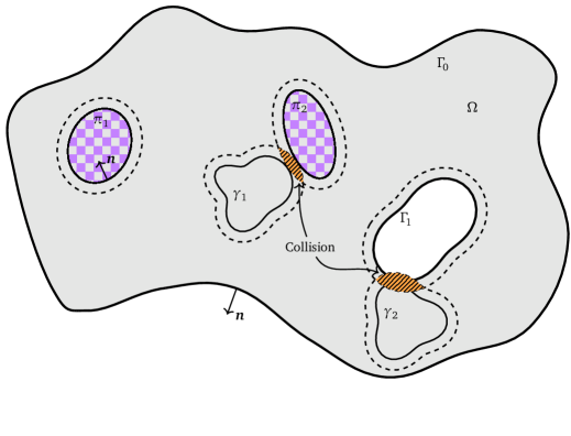
Figure 2: Schematic. The flow domain $\Omega$ (gray shaded area) with boundary $\Gamma_{k}~{}(k=0,\dots,K)$. Vesicles and rigid particles are suspended in the fluid. The vesicle boundaries are denoted by $\gamma_{i}~{}(i=1,\dots,N_{v})$ and the rigid particles (checkered pattern) are denoted by $\pi_{j}~{}(j=1,\dots,N_{p})$. The outward normal vector to the boundaries is denotes by $\bm{n}$. The dotted lines around boundaries denote the prescribed minimum separation distance for each of them. The minimum separation distance is a parameter and can be set to zero. In this schematic, vesicle $\gamma_{1}$ and particle $\pi_{2}$ as well as vesicle $\gamma_{2}$ and boundary $\Gamma_{1}$ are in contact. The slices of the space-time intersection volumes at the current instance are marked by  .

There are rigid particles suspended in the fluid domain. We denote the boundary of the j rigid particle by $\pi_{j}~{}(j=1,\dots,N_{p})$ and let $\pi\mathrel{\mathop{:}}=\bigcup_{j}\pi_{j}$. The governing equations are augmented with the no-slip boundary condition on the surface of vesicles and particles

$$\bm{u}(\bm{X},t) =\bm{X}_{t}\qquad(\bm{X}\in\gamma\cup\pi),$$ (2.3)

where $\bm{X}_{t}\mathrel{\mathop{:}}=\frac{\partial\bm{X}}{\partial t}$ is the material velocity of point $\bm{X}$ on the surface of vesicles or particles. The velocity on the fixed boundaries is imposed as a Dirichlet boundary condition

$$\bm{u}(\bm{x})=\bm{U}(\bm{x})\qquad(\bm{x}\in\Gamma).$$ (2.4)

We assume that the vesicle membrane is inextensible, i.e.,

$$\bm{X}_{s}\cdot\bm{u}_{s}=0\qquad(\bm{X}\in\gamma),$$ (2.5)

where the subscript “$s$” denotes differentiation with respect to the arclength on the surface of vesicles.

Rigid particles are typically force- and torque-free. However, surface forces may be exerted on them due to a constraint, e.g., the contact force $\bm{f}_{c}$, which we will define later. In this case, the force $\bm{F}^{\pi}_{j}$ and torque $L^{\pi}_{j}$ exerted on the j particle are the sum of such terms induced by constraints

$$\bm{F}^{\pi}_{j}=\bm{0},\quad\text{or}\quad \bm{F}^{\pi}_{j}=\int_{\pi_{j}}\bm{f}_{c}(\bm{X})\,\mathrm{d}s\qquad(j=1,\dots,N_{p}),$$ (2.6)

$$L^{\pi}_{j}=\bm{0},\quad\text{or}\quad L^{\pi}_{j}=\int_{\pi_{j}}(\bm{X}-\bm{c}^{\pi}_{j})\mathop{\cdot}{\bm{f}_{c}}^{\bot}(\bm{X})\,\mathrm{d}s\qquad(j=1,\dots,N_{p}),$$ (2.7)

where $\bm{c}^{\pi}_{j}$ is the center of mass for $\pi_{j}$ and for vector $\bm{f}=(f_{1},f_{2})$, ${\bm{f}}^{\bot}\mathrel{\mathop{:}}=(f_{2},-f_{1})$.

2.1 Contact definition

It is known [34, 18] that the exact solution of equations of motion, Eqs. 2.1, 2.3 and 2.4, keeps particles apart in finite time due to formation of lubrication film. Thus, it is theoretically sufficient to solve the equations with an adequate degree of accuracy to avoid any problems related to overlaps between particles. Nonetheless, achieving this accuracy for many types of flows (most notably, flows with high volume fraction of particles or with complex boundaries) may be prohibitively expensive.

With inadequate computational accuracy particles may collide with each other or with the boundaries and depending on the numerical method used, the consequences of this may vary. For methods based on integral equations the consequences are particularly dramatic, as overlapping boundaries may lead to divergent integrals. To address this issue, we augment the governing equations with a contact constraint, formally written as

$$V(S,t)\leq 0,$$ (2.8)

where $S=\Gamma\cup\gamma\cup\pi$ denotes the boundary of the domain and all particles. The function $V$ is chosen in a way that $V>0$ implies some parts of the surface $S$ are at a distance less than a user-specified constant $d_{m}$. Function $V$ may be a vector-valued function, for which the inequality is understood component-wise. This constraint ensures that the suspension remains contact-free independent of numerical resolution.

For the constraint function $V,$ in addition to the basic condition above, we choose a function that satisfies several additional criteria:

1. it introduces a relatively small number of additional constraints, and

2. when the function is discretized, no contacts are missed even for large time steps.

To clarify the second condition, suppose we have a small particle rapidly moving towards a planar boundary. For a large time step, it may move to the other side of the boundary in a single step, so any condition that considers an instantaneous quantity depending on only the current position is likely to miss the contact.

To this end, we use the Space-Time Interference Volumes (STIV) from [23] to define the function $V$ as the area in space-time swept by the intersecting segments of boundary over time. To be more precise, for each point $\bm{X}$ on the boundary $S$, consider a trajectory $\bm{X}(\tau)$, between a time $t_{0}$, for which there are no collisions, and a time $t$. Points $\bm{X}(\tau)$ define a deformed boundary $S(\tau)$ for each $\tau$. For each point $\bm{X}$, we define $\tau_{I}(\bm{X})$, $t_{0}\leq\tau_{I}\leq t$, to be the first instance for which this point comes into contact with a different point of $S(\tau_{I})$. We let $I(\bm{X})$ denote the point on $S(\tau_{I})$ that comes into contact with $\bm{X}(\tau_{I})$, i.e., $\bm{X}(\tau_{I})=I(\bm{X})(\tau_{I})$. For points which never come into contact with other points, we set $\tau_{I}=t$. Then, the space-time interference volume for 2d problems is defined as

$$V(S,t)=\int_{S(t_{0})}\int_{\tau_{I}(\bm{X})}^{t}\left[1+\big{(}\bm{X}_{t}(\tau)\mathop{\cdot}\bm{n}(\bm{X},\tau)\big{)}^{2}\right]^{1/2}\,\mathrm{d}\tau\,\mathrm{d}s$$ (2.9)

where $\bm{n}(\bm{X},\tau)$ denotes the normal to $S(\tau)$ at $\bm{X}(\tau)$. The integration is over the initial boundary $S(t_{0})$, and we use the fact that the surface is inextensible and the surface metric does not change. Note that, the term volume is a misnomer because Eq. 2.9 is the surface area swept by the intersecting segments of boundary. An important property of this choice of function, compared to, e.g., a space intersection volume, is that for even a very thin object moving at high velocity, it will be proportional to the time interval $t-t_{0}$.

We consider each connected component of this volume as a separate volume, and impose an inequality constraint on each; while keeping a single volume is in principle equivalent, using multiple volumes avoid certain undesirable effects in discretization [23]. Thus, $V(S,t)$ is a vector function of time-dependent dimension, with one component per active contact region.

Depending on the context, we may omit the dependence of $V$ on $S$ and write $V(t)$ as the contact volume function or $V(\gamma_{i},t)$ for the sub-vector of $V(S,t)$ involving surface $\gamma_{i}$.

In practice, it is desirable to control the minimal distance between particles. Therefore, we define a minimum separation distance $d_{m}\geq 0$ and modify the constraint such that particles are in contact when they are within $d_{m}$ distance from each other; as shown in Fig. 2. The contact volume with minimum separation distance is calculated with the surface displaced by $d_{m}$, i.e., the time $t_{I}$ is obtained not from the first contact with $S(\tau)$ but rather the displaced surface $S(\tau)+d_{m}\bm{n}(\tau)$. Maintaining minimum separation distance—rather than considering pure contact only—eliminates of potentially expensive computation of nearly singular integrals close to the surface and improves the accuracy in semi-explicit time-stepping.

2.2 Contact constraint

We use the Lagrange multiplier method (e.g., [60]) to add contact constraints to the system. While it is computationally more expensive than adding a penalty force for the constraint (effectively, an artificial repulsion force), it has the advantage of eliminating the need of tuning the parameters of the penalty force to ensure that the constraint is satisfied and keeping nonphysical forces introduced into the system to the minimum required for maintaining the desired separation. The constrained system can be written as

$$\min\int_{\Omega}\left(\frac{1}{2}\mu\operatorname{\nabla}\bm{u}\mathop{\cdot}\operatorname{\nabla}\bm{u}-\bm{u}\mathop{\cdot}\bm{F}\right)\,\mathrm{d}A,$$ (2.10)

$$\text{subject to:}\qquad\begin{aligned} \operatorname{\nabla\cdot}{\bm{u}}(\bm{x})&=0~{}~{}(\bm{x}\in\Omega),\\ \bm{X}_{s}\mathop{\cdot}\bm{u}_{s}&=0~{}~{}(\bm{X}\in\gamma),\\ V(S,t)&\geq 0.\\ \end{aligned}$$

If we omit the inequality constraint, the remaining three equations are equivalent to the Stokes equations (2.1). The Lagrangian for this system is

$$\mathcal{L}(\bm{u},p,\sigma,\lambda)=\int_{\Omega}\left(\frac{1}{2}\mu\operatorname{\nabla}\bm{u}\mathop{\cdot}\operatorname{\nabla}\bm{u}-\bm{u}\mathop{\cdot}\bm{F}-p\operatorname{\nabla\cdot}{\bm{u}}\right)\,\mathrm{d}A+\int_{\gamma}\sigma\bm{X}_{s}\mathop{\cdot}\bm{u}_{s}\,\mathrm{d}s+\lambda\mathop{\cdot}V.$$ (2.11)

The first-order optimality (KKT) conditions yield the following modified Stokes equation, along with the constraints listed in Eq. 2.10:

$$-\mu\Delta\bm{u}+\operatorname{\nabla}p=\bm{F}^{\prime},$$ (2.12)

$$\bm{F}^{\prime}=\bm{F}+\int_{\gamma}\bm{f}_{\sigma}\delta(\bm{x}-\bm{X})\,\mathrm{d}s+\int_{S}\bm{f}_{c}\delta(\bm{x}-\bm{X})\,\mathrm{d}s,$$ (2.13)

$$\bm{f}_{\sigma}=-(\sigma\bm{X}_{s})_{s},$$ (2.14)

$$\bm{f}_{c}=\operatorname{\nabla}V^{T}\lambda,$$ (2.15)

$$\lambda\geq 0,$$ (2.16)

$$\lambda\mathop{\cdot}V=0,$$ (2.17)

where the last condition is the complementarity condition—either an equality constraint is active $(V_{i}=0)$ or its Lagrange multiplier is zero. As we will see in the next section and based on Eq. 2.13, the collision force $\bm{f}_{c}$ is added to the traction jump across the vesicle’s interface. For rigid particles, the contact force induces force and torque on each particle—as given in Eqs. 2.6 and 2.7.

It is customary to combine $V\geq 0,\lambda\geq 0$, and $\lambda\mathop{\cdot}V=0$, into one expression and write

$$0\leq V(t)\quad\bot\quad\lambda\geq 0,$$ (2.18)

where "$\bot$" denotes the complementarity condition. These ensure that the Signorini conditions introduced in Section 1 are respected: contacts do not produce attraction force ($\lambda\geq 0$) and the constraint is active ($\lambda$ nonzero) if and only if $V(t)$ is zero. Furthermore, it follows from $V(t)\cdot\lambda=0$ that the contact force $\bm{f}_{c}$ is perpendicular to the velocity and therefore it respects the principal of virtual work and does not add to or remove from the system’s energy.

2.3 Boundary integral formulation

Following the standard approach of potential theory [42, 39], one can express the solution of the Stokes boundary value problem, Eq. 2.12, as a system of singular integro-differential equations on all immersed and bounding surfaces.

The Stokeslet tensor $\mathbf{G}$, the Stresslet tensor $\mathbf{T}$, and the Rotlet $\mathbf{R}$ are the fundamental solutions of the Stokes equation given by

$$\mathbf{G}(\bm{r}) =\frac{1}{4\pi\mu}\left(-\log\lVert\bm{r}\rVert\bm{I}+\frac{\bm{r}\otimes\bm{r}}{\lVert\bm{r}\rVert^{2}}\right),$$ (2.19)

$$\mathbf{T}(\bm{r}) =\frac{1}{\pi\mu}\frac{\bm{r}\otimes\bm{r}\otimes\bm{r}}{\lVert\bm{r}\rVert^{4}},$$ (2.20)

$$\mathbf{R}(\bm{r}) =\frac{1}{4\pi\mu}\frac{{\bm{r}}^{\bot}}{\lVert\bm{r}\rVert^{2}}.$$ (2.21)

The solution of Eq. 2.12 can be expressed by the combination of single- and double-layer integrals. We denote the single-layer integral on the vesicle surface $\gamma_{i}$ by

$$\mathcal{G}_{\gamma_{i}}[\bm{f}](\bm{x})\mathrel{\mathop{:}}=\int_{\gamma_{i}}\mathbf{G}(\bm{x}-\bm{Y})\cdot\bm{f}(\bm{Y})\,\mathrm{d}s,$$ (2.22)

where $\bm{f}$ is an appropriately defined density. The double-layer integral on a surface $S$ (a vesicle, a rigid particle, or a fixed boundary) is

$$\mathcal{T}_{S}[\bm{q}](\bm{x})\mathrel{\mathop{:}}=\int_{S}\bm{n}(\bm{Y})\cdot\mathbf{T}(\bm{x}-\bm{Y})\cdot\bm{q}(\bm{Y})\,\mathrm{d}s,$$ (2.23)

where $\bm{n}$ denotes the outward normal (as shown in Fig. 2) to the surface $S$, and $\bm{q}$ is appropriately defined density. When the evaluation point $\bm{x}$ is on the integration surface, Eq. 2.22 is a singular integral, and Eq. 2.23 is interpreted in the principal value sense.

Due to the linearity of the Stokes equations, as formulated in [50, 47], the velocity at a point $\bm{x}\in\Omega$ can be expressed as the superposition of velocities due to vesicles, rigid particles, and fixed boundaries

$$\alpha\bm{u}(\bm{x})=\bm{u}^{\infty}(\bm{x})+\bm{u}^{\gamma}(\bm{x})+\bm{u}^{\pi}(\bm{x})+\bm{u}^{\Gamma}(\bm{x}),\quad\bm{x}\in\Omega,\quad\alpha=\begin{cases}1&\bm{x}\in\Omega\backslash\gamma,\\ \nu_{i}&\bm{x}\in\varpi_{i},\\ (1+\nu_{i})/2&\bm{x}\in\gamma_{i},\end{cases}$$ (2.24)

where $\bm{u}^{\infty}(\bm{x})$ represent the background velocity field (for unbounded flows) and $\nu_{i}=\mu_{i}/\mu$ denotes the viscosity contrast of the i vesicle. The velocity contributions from vesicles, rigid particles, and fixed boundaries each can be further decomposed into the contribution of individual components

$$\bm{u}^{\gamma}(\bm{x}) =\sum_{i=1}^{N_{v}}\bm{u}_{i}^{\gamma}(\bm{x}), \bm{u}^{\pi}(\bm{x}) =\sum_{j=1}^{N_{p}}\bm{u}_{j}^{\pi}(\bm{x}), \bm{u}^{\Gamma}(\bm{x}) =\sum_{k=0}^{K}\bm{u}_{k}^{\Gamma}(\bm{x}).$$ (2.25)

To simplify the representation, we introduce the complementary velocity for each component. For the i vesicle, it is defined as $\bar{\bm{u}}^{\gamma}_{i}=\alpha\bm{u}-\bm{u}^{\gamma}_{i}$. The complementary velocity is defined in a similar fashion for rigid particles as well as components of the fixed boundary.

2.3.1.  The contribution from vesicles

The velocity induced by the i vesicle is expressed as an integral [42]:

$$\bm{u}_{i}^{\gamma}(\bm{x})=\mathcal{G}_{\gamma_{i}}[\bm{f}](\bm{x})+(1-\nu_{i})\mathcal{T}_{\gamma_{i}}[\bm{u}](\bm{x})\qquad(\bm{x}\in\Omega),$$ (2.26)

where the double-layer density $\bm{u}$ is the total velocity and $\bm{f}$ is the traction jump across the vesicle membrane. Based on Eq. 2.13, the traction jump is equal to the sum of bending, tensile, and collision forces

$$\bm{f}(\bm{X})=\bm{f}_{b}+\bm{f}_{\sigma}+\bm{f}_{c}=-\kappa_{b}\bm{X}_{ssss}-(\sigma\bm{X}_{s})_{s}+\operatorname{\nabla}V^{T}\lambda\qquad(\bm{X}\in\gamma),$$ (2.27)

where $\kappa_{b}$ is the membrane’s bending modulus. The tensile force $\bm{f}_{\sigma}=(\sigma\bm{X}_{s})_{s}$ is determined by the local inextensibility constraint, Eq. 2.5, and tension $\sigma$ is its Lagrangian multiplier.

Note that Eq. 2.26 is the contribution from each vesicle to the velocity field. To obtain an equation for the interfacial velocity, Eq. 2.26 is to be substituted into Eq. 2.24:

$$\frac{(1+\nu_{i})}{2}\bm{u}(\bm{X})=\bar{\bm{u}}_{i}^{\gamma}(\bm{X})+\mathcal{G}_{\gamma_{i}}[\bm{f}](\bm{X})+(1-\nu_{i})\mathcal{T}_{\gamma_{i}}[\bm{u}](\bm{X})\qquad(\bm{X}\in\gamma_{i}),$$ (2.28)

$$\bm{X}_{s}\cdot\bm{u}_{s}=0\qquad(\bm{X}\in\gamma_{i}).$$ (2.29)

2.3.2.  The contribution from the fixed boundaries

The velocity contribution from the fixed boundary can be expressed as a double-layer integral [39] along $\Gamma$. The contribution of the outer boundary $\Gamma_{0}$ is

$$\bm{u}_{0}^{\Gamma}(\bm{x})=\mathcal{T}_{\Gamma_{0}}[\bm{\eta_{0}}](\bm{x})\qquad(\bm{x}\in\Omega),$$ (2.30)

where $\bm{\eta}_{0}$ is the density to be determined based on boundary conditions. Substituting Eq. 2.30 into Eq. 2.24 and taking its limit to a point on $\Gamma_{0}$ and using the Dirichlet boundary condition, Eq. 2.4, we obtain a Fredholm integral equations for the density $\bm{\eta}_{0}$

$$\bm{U}(\bm{x})-\bar{\bm{u}}_{0}^{\Gamma}(\bm{x})=-\frac{1}{2}\bm{\eta}_{0}(\bm{x})+\mathcal{T}_{\Gamma_{0}}[\bm{\eta_{0}}](\bm{x})\qquad(\bm{x}\in\Gamma_{0}).$$

However, this equation is rank deficient. To render it invertible, the equation is modified following [42]:

$$\bm{U}(\bm{x})-\bar{\bm{u}}_{0}^{\Gamma}(\bm{x})=-\frac{1}{2}\bm{\eta}_{0}(\bm{x})+\mathcal{T}_{\Gamma_{0}}[\bm{\eta_{0}}](\bm{x})+\mathcal{N}_{\Gamma_{0}}[\bm{\eta_{0}}](\bm{x})\qquad(\bm{x}\in\Gamma_{0}),$$ (2.31)

where the operator $\mathcal{N}_{\Gamma_{0}}$ is defined as

$$\mathcal{N}_{\Gamma_{0}}[\bm{\eta_{0}}](\bm{x})=\int_{\Gamma_{0}}[\bm{n}(\bm{x})\otimes\bm{n}(\bm{y})]\mathop{\cdot}\bm{\eta_{0}}(\bm{y})\,\mathrm{d}s.$$ (2.32)

For the enclosed boundary components $\Gamma_{k}~{}(k>0)$ to eliminate the double-layer nullspace we need to include additional Stokeslet and Rotlet terms

$$\bm{u}_{k}^{\Gamma}(\bm{x})=\mathcal{T}_{\Gamma_{k}}[\bm{\eta_{k}}](\bm{x})+\mathbf{G}(\bm{x}-\bm{c}_{k}^{\Gamma})\cdot\bm{F}_{k}^{\Gamma}+\mathbf{R}(\bm{x}-\bm{c}_{k}^{\Gamma})L_{k}^{\Gamma},\qquad~{}(k=1,\dots,K;\bm{x}\in\Omega),$$ (2.33)

where $\bm{c}^{\Gamma}_{k}$ is a point enclosed by $\Gamma_{k}$, $\bm{F}_{k}^{\Gamma}$ is the force exerted on $\Gamma_{k}$, and $L_{k}^{\Gamma}$ is the torque:

$$\bm{F}_{k}^{\Gamma} =\frac{1}{|\Gamma_{k}|}\int_{\Gamma_{k}}\bm{\eta_{k}}\,\mathrm{d}s, L_{k}^{\Gamma} =\frac{1}{|\Gamma_{k}|}\int_{\Gamma_{k}}(\bm{X}-\bm{c}_{k}^{\Gamma})\mathop{\cdot}{\bm{\eta}}^{\bot}_{k}\,\mathrm{d}s,$$ (2.34)

where $|\Gamma_{k}|$ denotes the perimeter of $\Gamma_{k}$. Taking the limit at points of the surface, leads to the following integral equation:

$$\bm{U}(\bm{x})-\bar{\bm{u}}_{k}^{\Gamma}(\bm{x}) =-\frac{1}{2}\bm{\eta}_{k}(\bm{x})+\mathcal{T}_{\Gamma_{k}}[\bm{\eta_{k}}](\bm{x})+\mathbf{G}(\bm{x}-\bm{c}_{k}^{\Gamma})\cdot\bm{F}_{k}^{\Gamma}+\mathbf{R}(\bm{x}-\bm{c}_{k}^{\Gamma})L_{k}^{\Gamma}\qquad(\bm{x}\in\Gamma_{k}).$$ (2.35)

Equations 2.35 and 2.34 are a complete system for double-layer densities $\bm{\eta}_{k}$, forces $\bm{F}^{\Gamma}_{k}$, and torques $L_{k}^{\Gamma}$ on each enclosed surface $\Gamma_{k}$.

2.3.3.  The contribution from rigid particles

The formulation for rigid particles is very similar to that of fixed boundaries, except the force and torque are known (cf. Eqs. 2.6 and 2.7). The velocity contribution from the j rigid particle is

$$\bm{u}_{j}^{\pi}(\bm{x})=\mathcal{T}_{\pi_{j}}[\bm{\zeta}_{j}](\bm{x})+\bm{G}(\bm{x}-\bm{c}_{j}^{\pi})\cdot\bm{F}_{j}^{\pi}+\bm{R}(\bm{x}-\bm{c}_{j}^{\pi})L_{j}^{\pi},$$ (2.36)

Where $\bm{F}_{j}^{\pi},L_{j}^{\pi}$ are, respectively, the known net force and torque exerted on the particle and $\bm{\zeta}_{j}$ is the unknown density.

Let $\bm{U}_{j}^{\pi}$ and $\omega_{j}^{\pi}$ be the translational and angular velocities of the j particle; then we obtain the following integral equation for the density $\bm{\zeta}_{j}$ from the limit of (2.36):

$$\bm{U}_{j}^{\pi}+\omega_{j}^{\pi}{(\bm{X}-\bm{c}_{j}^{\pi})}^{\bot}-\bar{\bm{u}}^{\pi}_{j}(\bm{X})=-\frac{1}{2}\bm{\zeta}_{j}(\bm{X})+\mathcal{T}_{\pi_{j}}[\bm{\zeta}_{j}](\bm{X})+\bm{G}(\bm{X}-\bm{c}_{j}^{\pi})\cdot\bm{F}_{j}^{\pi}+\bm{R}(\bm{X}-\bm{c}_{j}^{\pi})L_{j}^{\pi}.$$ (2.37)

where

$$\bm{F}_{j}^{\pi} =\frac{1}{|\pi_{j}|}\int_{\pi_{j}}\bm{\zeta}_{j}\,\mathrm{d}s, L_{j}^{\pi} =\frac{1}{|\pi_{j}|}\int_{\pi_{j}}(\bm{Y}-\bm{c}_{j}^{\pi})\mathop{\cdot}{\bm{\zeta}}^{\bot}_{j}\,\mathrm{d}s$$ (2.38)

where $\bm{c}_{j}^{\pi}$ is the center of $\engordnumber{j}$ rigid particle. Equations 2.37 and 2.38 are used to solve for the unknown densities $\bm{\zeta}_{j}$ as well as the unknown translational and angular velocities of each particle. Note that the objective of Eqs. 2.34 and 2.38 is remove the null space of the double-layer and therefore the left-hand-side (i.e. the image of the null function) can be chosen rather arbitrarily.

2.4 Formulation summary

The formulae outlined above govern the evolution of the suspension. The flow constituents are hydrodynamically coupled through the complementary velocity (i.e., the velocity from all other constituents). Given the configuration of the suspension, the unknowns are:

• Velocity $\bm{u}(\bm{X})$ and tension $\sigma$ of vesicles’ interface determined by Eqs. 2.27, 2.28 and 2.29. The velocity is integrated for the vesicles’ trajectory using Eq. 2.3.

• The double-layer density on the enclosing boundary $\bm{\eta}_{0}$ as well as the double-layer density $\bm{\eta}_{k}~{}(k=1,\dots,K)$, force $\bm{F}_{k}^{\Gamma}$, and torque $L_{k}^{\Gamma}$ on the interior boundaries determined by Eqs. 2.31, 2.35 and 2.34. Note that the collision constraint does not enter the formulation for the fixed boundaries and when a particle collides with a fixed boundary, the collision force is only applied to the particle. The unknown force and torque above can be interpreted as the required force to keep the boundary in place.

• Translational $\bm{U}_{j}^{\pi}$ and angular $\omega_{j}^{\pi}$ velocities of rigid particles $(j=1,\dots,N_{p})$ as well as double-layer densities $\bm{\zeta}_{j}$ on their boundary determined by Eqs. 2.37 and 2.38. Where the force and torque are either zero or determined by the collision constraint Eqs. 2.6 and 2.7.

This system is constrained by Signorini (KKT) conditions for the contact, Eq. 2.18, which is used to compute $\lambda$, the strength of the contact force.

In the referenced equations above, the complementary velocity is combination of velocities given in Eqs. 2.26, 2.30, 2.33 and 2.36.

3 Discretization and Numerical Methods

In this section, we describe the numerical algorithms required for solving the dynamics of a particulate Stokesian suspension. We use the spatial representation and integral schemes in [50]. We also adapt the spectral deferred correction time-stepping in [49, 48] to the local implicit time-stepping schemes. Furthermore, we use piecewise-linear discretization of curves to calculate the space-time contact volume $V(\gamma,t)$, Eq. 2.9, as in [23]. To solve the complementarity problem resulting from the contact constraint, we use the minimum-map Newton method discussed in [13].

The key difference, compared to previous works is that at every time step instead of solving a linear system we solve a nonlinear complementarity problem (NCP). The NCPs are solved iteratively, using a Linear Complementarity Problem (LCP) solver. We refer to these iterations as contact-resolving iterations, in contrast to the outer time-stepping iterations.

For simplicity, we describe the scheme for a system including vesicles only, without boundaries or rigid particles. Adding these requires straightforward modifications to the equations. In the following sections, we will first summarize the spatial discretization, then discuss the LCP solver, and close with the time discretization with contact constraint.

3.1 Spatial discretization

All interfaces are discretized with $N$ uniformly-spaced discretization points [50]. The number of points on each curve is typically different but for the sake of clarity we use $N$. The distance between discretization points does not change with time over the curves due to rigidity of particles or the local inextensibility constraint for vesicles. Let $\bm{X}(s)$, with $s\in(0,L]$, be a parametrization of the interface $\gamma_{i}~{}(\text{or}~{}\pi_{j})$, and let $\{s_{k}=kL/N\}_{k=1}^{N}$ be $N$ equally spaced points in arclength parameter, and $\bm{\mathsf{X}}_{k}\mathrel{\mathop{:}}=\bm{X}(s_{k})$ the corresponding material points.

High-order discretization for force computation

We use the Fourier basis to interpolate the positions and forces associated with sample points, and FFT to calculate the derivatives of all orders to spectral accuracy. We use the hybrid Gauss-trapezoidal quadrature rules of [3] to integrate the single-layer potential for $\bm{X}\in\gamma_{i}$

$$\mathcal{G}_{\gamma_{i}}[\bm{f}](\bm{X})\approx\bm{\mathsf{G}}_{\gamma_{i}}[\bm{\mathsf{f}}](\bm{\mathsf{X}})\mathrel{\mathop{:}}=\sum_{\ell=1}^{N+M}w_{\ell}\bm{\mathsf{G}}(\bm{\mathsf{X}}-\bm{\mathsf{Y}}_{\ell})\mathop{\cdot}\bm{\mathsf{f}}(\bm{\mathsf{Y}}_{\ell}),$$ (3.1)

where $w_{\ell}$ are the quadrature weights given in [3, Table 8] and $\bm{\mathsf{Y}}_{\ell}$ are quadrature points. For $\bm{X}\in\gamma_{i}$, the linear operator $\bm{\mathsf{G}}_{\gamma_{i}}$ is a matrix, we denote the single-layer potential on $\gamma_{i}$ as $\bm{\mathsf{G}}_{\gamma_{i}}\bm{\mathsf{f}}$.

The double-layer kernel $\bm{n}(\bm{Y})\mathop{\cdot}\mathbf{T}(\bm{X}-\bm{Y})$ in Eq. 2.23 is non-singular in two dimensions

$$\lim_{\gamma_{i}\ni\bm{X}\to\bm{Y}}\bm{n}(\bm{Y})\cdot\mathbf{T}(\bm{X}-\bm{Y})=-\frac{\kappa}{2\pi\mu}\bm{t}\otimes\bm{t},$$

where $\bm{t}$ denotes the tangent vector. Therefore, a simple uniform-weight composite trapezoidal quadrature rule has spectral accuracy in this case. Similar to the single-layer case, we denote the discrete double-layer potential on $\gamma_{i}$ by $\bm{\mathsf{T}}_{\gamma_{i}}\bm{\mathsf{u}}$. We use the nearly-singular integration scheme described in [47] to maintain high integration accuracy for particles closely approaching each other.

Piecewise-linear discretization for constraints.

While the spectral spatial discretization is used for most computations, it poses a problem for the minimal-separation constraint discretization. Computing parametric curve intersections, an essential step in the STIV computation, is relatively expensive and difficult to implement robustly, as this requires solving nonlinear equations. We observe that the impact of the separation distance on the overall accuracy is low in most situations, as explored in Section 4. Thus, rather than enforcing the constraint as precisely as allowed by the spectral discretization, we opt for a low-order, piecewise-linear discretization in this case, and use an algorithm that ensures that at least the target minimal separation is maintained, but may enforce a higher separation distance.

For the purpose of computing STIV and its gradient, we use $L(\bm{\mathsf{X}},r)$, the piecewise-linear interpolant of $r$ times refinement of points—the upsampled points correspond to arclength values with spacing $L/(N2^{r})$, with $r$ determined dynamically.

For discretized computations, we set the separation distance to $(1+2\alpha)d_{m}$, where $d_{m}$ is the target minimum separation distance. We choose $r$ such that $\lVert L(\bm{\mathsf{X}},r)-\bm{X}\rVert_{\infty}<\alpha d_{m}$. Our NCP solver, described below, ensures that the separation between $L(\bm{\mathsf{X}},r)$ is $(1+2\alpha)d_{m}$ at the end of a single time step. We choose $\alpha=0.1$ which requires $r=1$ in our experiments; smaller values of $\alpha$ require more refinement, but enforce the constraint more accurately.

At the end of the time step, the minimal-separation constraint ensures that $L(\bm{\mathsf{X}},r)(s)$, for any $s$, is at least at the distance $(1+2\alpha)d_{m}$ from a possible intersection if its trajectory is extrapolated linearly. By computing the upper bounds on the difference between the $\bm{X}(s)$ and $L(\bm{\mathsf{X}},r)(s)$ at the beginning of the time step, and interpolated velocities, we obtain a lower bound on the actual separation distance $d^{\prime}$ for the spectral surface $\bm{X}(s)$. If $d^{\prime}<d_{m}$, we increase $r$, and repeat the time step. As the piecewise linear approximation converges to the spectral boundary $\bm{X}$, and so do the interpolated velocities. In practice, we have not observed a need for refinement for our choice of $\alpha$.

For the piecewise-linear discretization of curves, the space-time contact volume $V(\gamma,t)$, Eq. 2.9, and its gradient are calculated using the definitions and algorithms in [23]. Given a contact-free configuration and a candidate configuration for the next time step, we calculate the discretized space-time contact volume as the sum of edge-vertex contact volumes $V=\sum_{k}V_{k}(\bm{\mathsf{e}},\bm{\mathsf{X}})$. We use a regular grid of size proportional to the average boundary spacing to quickly find potential collisions. For all vertices and edges, the bounding box enclosing their initial (collision-free) and final (candidate position) location is formed and all the grid boxes intersecting that box are marked. When the minimal separation distance $d_{m}>0$, the bounding box is enlarged by $d_{m}$. For each edge-vertex pair $\bm{\mathsf{e}}(\bm{\mathsf{X}}_{i},\bm{\mathsf{X}}_{i+1})$ and $\bm{\mathsf{X}}_{j}$, we solve a quartic equation to find their earliest contact time $\tau_{I}$ assuming linear trajectory between initial and candidate positions. We calculate the edge-vertex contact volume using Eq. 2.9:

$$V_{k}(\bm{\mathsf{e}},\bm{\mathsf{X}})=(t-\tau_{I})(1+(\bm{\mathsf{X}}(\tau_{I})\cdot\bm{\mathsf{n}}(\tau_{I}))^{2})^{1/2}|\bm{e}|,$$ (3.2)

where $\bm{\mathsf{n}}(\tau_{I})$ is the normal to the edge $\bm{\mathsf{e}}(\tau_{I})$. For each edge-vertex contact volume, we calculate the gradient respect to the vertices $\bm{\mathsf{X}}_{i}$, $\bm{\mathsf{X}}_{i+1}$ and $\bm{\mathsf{X}}_{j}$, summing over all the edge-vertex contact pairs we get the total space-time contact volume and gradient.

3.2 Temporal discretization

Our temporal discretization is based on the locally-implicit time-stepping scheme in [50]—adapting the Implicit–Explicit (IMEX) scheme [4] for interfacial flow—in which we treat intra-particle interactions implicitly and inter-particle interactions explicitly. We combine this method with the minimal-separation constraint. We refer to this scheme as constrained locally-implicit (CLI) scheme. For comparison purposes, we also consider the same scheme without constraints (LI) and the globally semi-implicit (GI) scheme, where all interactions treated implicitly [51]. From the perspective of boundary integral formulation, the distinguishing factor between LI and CLI is the extra traction jump term due to collision. Schemes LI/CLI and GI differ in their explicit or implicit treatment of the complementary velocities.

While treating the inter-vesicle interactions explicitly may result in more frequent violations of minimal-separation constraint, we demonstrate that in essentially all cases the CLI scheme is significantly more efficient than both the GI and LI schemes because these schemes are costlier and require higher spatial and temporal resolution to prevent collisions.

We consider two versions of the CLI scheme, a simple first-order Euler scheme and a spectral deferred correction version. A first-order backward Euler CLI time stepping formulation for Eq. 2.28 is

$$\frac{1+\nu_{i}}{2}\bm{\mathsf{u}}_{i}^{+} =\bar{\bm{\mathsf{u}}}_{i}^{\gamma}+\bm{\mathsf{G}}_{\gamma_{i}}\bm{\mathsf{f}}_{i}(\bm{\mathsf{X}}_{i}^{+},\sigma_{i}^{+},\lambda^{+})+(1-\nu_{i})\bm{\mathsf{T}}_{\gamma_{i}}\bm{\mathsf{u}}_{i}^{+},$$ (3.3)

$$\bm{\mathsf{X}}_{i,s}\mathop{\cdot}\bm{\mathsf{u}}_{i,s}^{+} =0,$$ (3.4)

$$\bm{\mathsf{f}}_{i}(\bm{\mathsf{X}}_{i}^{+},\sigma_{i}^{+},\lambda^{+}) =-\kappa_{b}\bm{\mathsf{X}}_{i,ssss}^{+}-(\sigma^{+}\bm{\mathsf{X}}_{i,s})_{s}+((\operatorname{\nabla}\mathsf{V}^{+})^{T}\lambda^{+})_{i},$$ (3.5)

$$0\leq\mathsf{V}(\gamma;t^{+})\quad \bot\quad\lambda^{+}\geq 0,$$ (3.6)

where the implicit unknowns to be solved for at the current step are marked with superscript “⁺”. The position and velocity of the points of $\engordnumber{i}$ vesicle are denoted by $\bm{\mathsf{X}}_{i}$, $\bm{\mathsf{u}}_{i}^{+}=(\bm{\mathsf{X}}_{i}^{+}-\bm{\mathsf{X}}_{i})/\Delta t$, and $\bm{\mathsf{f}}_{i}$ is the traction jump on the $\engordnumber{i}$ vesicle boundary. $\mathsf{V}(\gamma;t^{+})$ is the STIV function.

3.2.1.  Spectral Deferred Correction

We use spectral deferred correction (SDC) method [49, 48] to get a better stability behavior compared to the basic backward Euler scheme described above. We use SDC both for LI and CLI time-stepping. To obtain the SDC time-stepping equations, we reformulate Eq. 2.3 as a Picard integral

$$\bm{X}(t_{n+1})=\bm{X}(t_{n})+\int_{t_{n}}^{t_{n+1}}\bm{u}\left(\bm{X}(\tau),\sigma(\tau),\lambda(\tau)\right)\,\mathrm{d}\tau,$$ (3.7)

where the velocity satisfies Eqs. 2.28 and 3.3. In the SDC method, the integral in Eq. 3.7 is first discretized with $p+1$ Gauss-Lobatto quadrature points. Each iteration starts with $p$ provisional positions $\widetilde{\bm{\mathsf{X}}}$ corresponding to times $\tau_{i}$ in the interval $[t_{n},t_{n+1}]$; $t_{n}=\tau_{0}<\cdots<\tau_{p}=t_{n+1}$. Provisional tensions $\widetilde{\mathsf{\sigma}}$ and provisional $\widetilde{\mathsf{\lambda}}$ are defined similarly. The SDC method iteratively corrects the provisional positions $\widetilde{\bm{\mathsf{X}}}$ with the error term $\widetilde{\bm{\mathsf{e}}}$, which is solved using the residual $\widetilde{\bm{\mathsf{r}}}$ resulting from the provisional solution as defined below. The residual is given by:

$$\widetilde{\bm{r}}(\tau)=\widetilde{\bm{X}}(t_{n})-\widetilde{\bm{X}}(\tau)+\int_{t_{n}}^{\tau}\widetilde{\bm{u}}(\theta)\,\mathrm{d}\theta.$$ (3.8)

After discretization, we use $\widetilde{\bm{\mathsf{X}}}^{w,m}$, to denote the provisional position at m Gauss-Lobatto point after $w$ SDC passes. The error term $\widetilde{\bm{\mathsf{e}}}^{w,m}$ denotes the computed correction to obtain m provisional position in w iteration. The SDC correction iteration is defined by

$$\widetilde{\bm{\mathsf{X}}}^{w,m} =\widetilde{\bm{\mathsf{X}}}^{w-1,m}+\widetilde{\bm{\mathsf{e}}}^{w,m},$$

$$\widetilde{\sigma}^{w,m} =\widetilde{\mathsf{\sigma}}^{w-1,m}+\widetilde{\mathsf{e}}^{w,m}_{\sigma},$$ (3.9)

$$\widetilde{\lambda}^{w,m} =\widetilde{\mathsf{\lambda}}^{w-1,m}+\widetilde{\mathsf{e}}^{w,m}_{\lambda}.$$

Setting $\widetilde{\bm{\mathsf{X}}}^{0,m}$ to zero, the first SDC pass is just backward Euler time stepping to obtain nontrivial provisional solutions. Beginning from the second pass, we solve for the error term as corrections.

Denote $(\alpha\bm{\mathsf{I}}-(1-\nu)\bm{\mathsf{T}}_{\widetilde{\gamma}^{w-1,m}})$ by $\bm{\mathsf{D}}_{\widetilde{\gamma}^{w-1,m}}$. Following [49, 48], we solve the following equation for the error term:

$$\alpha\frac{\widetilde{\bm{\mathsf{e}}}^{w,m}-\widetilde{\bm{\mathsf{e}}}^{w,m-1}}{\Delta\tau}=\bm{\mathsf{D}}_{\widetilde{\gamma}^{w-1,m}}\left(\frac{\widetilde{\bm{\mathsf{r}}}^{w-1,m}-\widetilde{\bm{\mathsf{r}}}^{w-1,m-1}}{\Delta\tau}\right)+\bm{\mathsf{G}}_{\widetilde{\gamma}^{w-1,m}}\bm{\mathsf{f}}(\widetilde{\bm{\mathsf{e}}}^{w,m},\widetilde{\mathsf{e}}^{w,m}_{\sigma},\widetilde{\mathsf{e}}^{w,m}_{\lambda})+(1-\nu)\bm{\mathsf{T}}_{\widetilde{\gamma}^{w-1,m}}\left(\frac{\widetilde{\bm{\mathsf{e}}}^{w,m}-\widetilde{\bm{\mathsf{e}}}^{w,m-1}}{\Delta\tau}\right).$$ (3.10)

Eq. 3.10 is the identical to Eq. 3.3, except the right-hand-side for Eq. 3.10 is obtained from the residual while the right-hand-side for Eq. 3.3 is the complementary velocity. The residual $\widetilde{\bm{\mathsf{r}}}^{w,m}$ is obtained using a discretization of Eq. 3.8:

$$\widetilde{\bm{\mathsf{r}}}^{w,m}=\widetilde{\bm{\mathsf{X}}}^{w,0}-\widetilde{\bm{\mathsf{X}}}^{w,m}+\sum_{l=0}^{p}w_{l,m}\widetilde{\bm{\mathsf{u}}}^{w,l}.$$ (3.11)

where $w_{l,m}$ are the quadrature weights for Gauss-Lobatto points, whose quadrature error is $\mathcal{O}(\Delta t^{2p-3})$. In addition to the SDC iteration, Eq. 3.10, we also enforce the inextensibility constraint

$$\widetilde{\bm{\mathsf{X}}}^{w-1,m}_{s}\cdot\widetilde{\bm{\mathsf{u}}}^{w,m}_{s}=0,$$ (3.12)

and the contact complementarity

$$0\leq\mathsf{V}(\widetilde{\gamma}^{w,m})\quad\bot\quad\widetilde{\mathsf{e}}_{\lambda}^{w,m}\geq 0.$$ (3.13)

In evaluating the residuals using Eq. 3.11, provisional velocities are required. In the GI scheme [49], all the interactions are treated implicitly and given provisional position $\widetilde{\bm{\mathsf{X}}}^{w,m}$, the provisional velocities are obtained by evaluating

$$\widetilde{\bm{\mathsf{u}}}^{w,m}=\bm{\mathsf{D}}_{\widetilde{\gamma}^{w,m}}^{-1}\left(\bm{\mathsf{G}}_{\widetilde{\gamma}^{w,m}}\bm{\mathsf{f}}(\widetilde{\bm{\mathsf{X}}}^{w,m},\widetilde{\mathsf{\sigma}}^{w,m},\widetilde{\mathsf{\lambda}}^{w,m})+\bm{\mathsf{u}}^{\infty}\right).$$ (3.14)

which requires a global inversion of $\bm{\mathsf{D}}_{\widetilde{\gamma}^{w,m}}$. The same approach is taken for LI and CLI schemes, except the provisional velocities are obtained using local inversion only, all the inter-particle interactions are treated explicitly and added to the explicit term, i.e., complementary velocity $\widetilde{\bar{\bm{\mathsf{u}}}}_{i}^{w-1,m}$; modifying Eq. 3.14 for each vesicle, we obtain

$$\widetilde{\bm{\mathsf{u}}}_{i}^{w,m}=\bm{\mathsf{D}}_{\widetilde{\gamma}_{i}^{w,m}}^{-1}\left(\bm{\mathsf{G}}_{\widetilde{\gamma}_{i}^{w,m}}\bm{\mathsf{f}}(\widetilde{\bm{\mathsf{X}}}_{i}^{w,m},\widetilde{\mathsf{\sigma}}^{w,m}_{i},\widetilde{\mathsf{\lambda}}^{w,m}_{i})+\widetilde{\bar{\bm{\mathsf{u}}}}_{i}^{w-1,m}\right),$$ (3.15)

where $\widetilde{\bar{\bm{\mathsf{u}}}}_{i}^{w-1,m}$ is computed using $\widetilde{\bm{\mathsf{X}}}^{w,m}$ and $\widetilde{\bm{\mathsf{u}}}_{j}^{w-1,m}$($j\neq i$) accounting the velocity influence from other vesicles. We only need to invert the local interaction matrices $\bm{\mathsf{D}}_{\widetilde{\gamma}_{i}^{w,m}}$ in this scheme.

3.2.2.  Contact-resolving iteration

Let $\bm{\mathsf{A}}\bm{\mathsf{X}}^{+}=\bm{\mathsf{b}}$ be the linear system that is solved at each iteration of a CLI scheme (in case of the CLI-SDC scheme, on each of the inner step of the SDC). $\bm{\mathsf{A}}$ is a block diagonal matrix, with blocks $\bm{\mathsf{A}}_{ii}$ corresponding to the self interactions of the $\engordnumber{i}$ particle. All inter-particle interactions are treated explicitly, and thus included in the right-hand side $\bm{\mathsf{b}}$. We write Eq. 3.3, or Eq. 3.10, in a compact form as

$$\bm{\mathsf{A}}\bm{\mathsf{X}}^{+} =\bm{\mathsf{b}}+\bm{\mathsf{G}}\bm{\mathsf{f}}_{c}^{+},$$ (3.16)

$$0\leq\mathsf{V}(\mathsf{\gamma};t^{+})\quad \bot\quad\mathsf{\lambda}\geq 0,$$ (3.17)

which is a mixed Nonlinear Complementarity Problem (NCP), because the STIV function $\mathsf{V}(\mathsf{\gamma},t)$ is a nonlinear function of position. Note that since this is the CLI scheme, $\bm{\mathsf{G}}$ is also a block diagonal matrix. To solve this NCP, we use a first-order linearization of the $\mathsf{V}(\mathsf{\gamma};t)$ to obtain an LCP and iterate until the NCP is solved to the desired accuracy:

$$\bm{\mathsf{A}}\bm{\mathsf{X}}^{\star}=\bm{\mathsf{b}}+\bm{\mathsf{G}}\bm{\mathsf{J}}^{T}\mathsf{\lambda}.$$ (3.18)

$$0\leq\mathsf{V}(\mathsf{\gamma};t^{+k})+\bm{\mathsf{J}}\Delta\bm{\mathsf{X}}\quad\bot\quad\mathsf{\lambda}\geq 0,$$ (3.19)

where $\Delta\bm{\mathsf{X}}$ is the update to get the new candidate solution $\bm{\mathsf{X}}^{\star}$, and $\bm{\mathsf{J}}$ denotes the Jacobian of the volume $\nabla_{X}\mathsf{V}(\mathsf{\gamma},t^{+k})$. Algorithm 1 summarizes the steps to solve Eqs. 3.16 and 3.17 as a series of linearization steps Eqs. 3.18 and 3.19. We discuss the details of the LCP solver separately below.

input : $\bm{\mathsf{X}},\bm{\mathsf{b}}$

output : $\bm{\mathsf{X}}^{+},\bm{\mathsf{f}}_{c}^{+}$

1 $\bm{\mathsf{A}}\leftarrow\bm{\mathsf{A}}(\bm{\mathsf{X}})$

2 $\bm{\mathsf{b}}\leftarrow\bm{\mathsf{b}}(\bm{\mathsf{X}})$

3 $\bm{\mathsf{f}}_{c}^{+}\leftarrow 0$

4 $k\leftarrow 0$

5 $\bm{\mathsf{X}}^{\star}\leftarrow\bm{\mathsf{A}}^{-1}\bm{\mathsf{b}}$

6 $\mathsf{V}\leftarrow$ getContactVolume($\bm{\mathsf{X}}^{\star}$)

7while $\mathsf{V}<0$ do

8       $\bm{\mathsf{J}}\leftarrow$ getContactVolumeJacobi($\bm{\mathsf{X}}^{\star}$)

9      $\lambda\leftarrow$ lcpSolver($\mathsf{V}$)

10       $k\leftarrow k+1$

11       $\bm{\mathsf{b}}\leftarrow\bm{\mathsf{b}}+\bm{\mathsf{GJ}}^{T}\lambda$

12       $\bm{\mathsf{X}}^{\star}\leftarrow\bm{\mathsf{A}}^{-1}\bm{\mathsf{b}}$

13       $\mathsf{V}\leftarrow$ getContactVolume($\bm{\mathsf{X}}^{\star}$)

14      $\bm{\mathsf{f}}_{c}^{+}\leftarrow\bm{\mathsf{f}}_{c}^{+}+\bm{\mathsf{J}}^{T}\lambda$

15      

16$\bm{\mathsf{X}}^{+}\leftarrow\bm{\mathsf{X}}^{\star}$

Algorithm 1 Contact-free time-stepping.

In lines $1$ to $6$, we solve the unconstrained system $\bm{\mathsf{A}}\bm{\mathsf{X}}^{\star}=\bm{\mathsf{b}}$ using the solution from previous time step. Then, the STIVs are computed to check for collision. The loop at lines $7{-}14$ is the linearized contact-resolving steps. Substituting Eq. 3.18 into Eq. 3.19, and using the fact that $\Delta\bm{\mathsf{X}}=\bm{\mathsf{A}}^{-1}\bm{\mathsf{GJ}}^{T}\lambda$ we cast the problem in the standard LCP form

$$0\leq\mathsf{V}+\bm{\mathsf{B}}\mathsf{\lambda}\quad\bot\quad\mathsf{\lambda}\geq 0,$$ (3.20)

where $\bm{\mathsf{B}}=\bm{\mathsf{JA}}^{-1}\bm{\mathsf{GJ}}^{T}$. The LCP solver is called on line $9$ to obtain the magnitude of the constraint force, which is in turn used to update obtain new candidate positions that may or may not satisfy the constraints. Line $13$ checks the minimal-separation constraints for the candidate solution. In line 11, the collision force is incorporated into the right-hand-side $\bm{\mathsf{b}}$ for self interaction in the next LCP iteration. In line 14, the contact force is updated, which will be used to form the right-hand-side $\bm{\mathsf{b}}$ for the global interaction in the next time step.

The LCP matrix $\bm{\mathsf{B}}$ is an $M$ by $M$ matrix, where $M$ is the number of contact volumes, $M=\mathcal{O}(N_{v}+N_{p})$. Each entry $\bm{\mathsf{B}}_{k,p}$ is induced change in the $\engordnumber{k}$ contact volume by the p contact force. Matrix $\bm{\mathsf{B}}$ is sparse and typically diagonally dominant, since most STIV volumes are spatially separated.

3.3 Solving the Linear Complementarity Problem

In the contact-resolving iterations we solve an LCP, Eq. 3.20. Most common algorithms (e.g., Lemke’s algorithm [28] and splitting based iterative algorithms [31, 1]) requires explicitly formed LCP matrix $\bm{\mathsf{B}}$, which can be prohibitively expensive when there are many collisions. We use the minimum-map Newton method, which we modify to require matrix-vector evaluation only, as we can perform it without explicitly forming the matrix.

We briefly summarize the minimum-map Newton method. Let $\bm{\mathsf{y}}=\mathsf{V}+\bm{\mathsf{B}}\lambda$. Using the minimum map reformulation we can convert the LCP to a root-finding problem

$$\bm{\mathsf{H}}(\mathsf{\lambda})\equiv\begin{bmatrix}h(\lambda_{1},y_{1})\\ \cdots\\ h(\lambda_{M},y_{M})\end{bmatrix}=0,$$ (3.21)

where $h(\lambda_{i},y_{i})=\min(\lambda_{i},y_{i})$. This problem is solved by Newton’s method (Algorithm 2). In the algorithm, $\bm{\mathsf{P}}_{\mathbb{A}}$ and $\bm{\mathsf{P}}_{\mathbb{F}}$ are selection matrices: $\bm{\mathsf{P}}_{\mathbb{A}}\lambda$ selects the rows of $\mathsf{\lambda}$ whose indices are in set $\mathbb{A}$ and zeros out all the other rows. While function $\bm{\mathsf{H}}$ is not smooth, it is Lipschitz and directionally differentiable, and its so-called B-derivative $\bm{\mathsf{P}}_{\mathbb{A}}\bm{\mathsf{B}}+\bm{\mathsf{P}}_{\mathbb{F}}$ can be formed to find the descent direction for Newton’s method [13]. The matrix $\bm{\mathsf{P}}_{\mathbb{A}}\bm{\mathsf{B}}+\bm{\mathsf{P}}_{\mathbb{F}}$ is a sparse matrix, and we use GMRES to solve this linear system. Since $\bm{\mathsf{B}}$ is sparse and diagonally dominant, in practice the linear system is solved in few GMRES iterations and the Newton solver converges quadratically.

require : $\textnormal{{applyLCPMatrix}}()$, $\mathsf{V}$ and $\epsilon$

output : $\lambda$

1 $e\leftarrow\epsilon$

2 $\lambda\leftarrow 0$

3 while $e>\epsilon$ do

4       $\bm{\mathsf{y}}\leftarrow\mathsf{V}+\text{{{applyLCPMatrix(}}{\emph{$\lambda$}}{{)}}}$

5       $\mathbb{A}\leftarrow\left\{i\middle|y_{i}<\lambda_{i}\right\}$

6        // index of active constraints

7       $\mathbb{F}\leftarrow\left\{i\middle|y_{i}\geq\lambda_{i}\right\}$

8       Iteratively solve $\displaystyle\begin{bmatrix}\bm{\mathsf{B}}&\bm{\mathsf{-I}}\\ \bm{\mathsf{P}}_{\mathbb{F}}&\bm{\mathsf{P}}_{\mathbb{A}}\end{bmatrix}\begin{bmatrix}\Delta\lambda\\ \Delta y\end{bmatrix}=\begin{bmatrix}0\\ -\bm{\mathsf{P}}_{\mathbb{A}}\bm{\mathsf{y}}-\bm{\mathsf{P}}_{\mathbb{F}}\mathsf{\lambda}\end{bmatrix}$

9        // $\bm{\mathsf{B}}$ applied by applyLCPMatrix

10       $\tau\leftarrow$ projectLineSearch($\Delta\lambda$)

11       $\lambda\leftarrow\lambda+\tau\Delta\lambda$

12       $e\leftarrow\lVert\bm{\mathsf{H}}(\lambda)\rVert$

Algorithm 2 Minimum Map LCP Solver.

3.4 Algorithm Complexity

We estimate the complexity of a single time step as a function of the number of points on each vesicle $N$, number of vesicles $N_{v}$. Let $C_{N}$ denote the cost of inverting a local linear system for one particle; then the complexity of inverting linear systems for all particles is $\mathcal{O}\left(C_{N}N_{v}\right)$. In [58, 50] it is shown that for LI scheme $C_{N}=\mathcal{O}\left(N\log N\right)$. The cost of evaluating the inter-particle interactions at the $N_{v}N$ discrete points using FMM is $\mathcal{O}(N_{v}N)$.

We assume that for each contact resolving step, the number of contact volumes is $M$. Assuming that minimum map Newton method takes $K_{1}$ steps to converge, the cost of solving the LCP is $\mathcal{O}\left(K_{1}C_{N}N_{v}\right)$, because inverting $\bm{\mathsf{A}}$ is the costliest step in applying the LCP matrix. The total cost of solving the NCP problem is $\mathcal{O}\left(K_{1}K_{2}C_{N}N_{v}\right)$, where $K_{2}$ are the number of contact resolving iterations. In the numerical simulations we observe that the minimum map Newton method converges in a few iterations ($K_{1}\approx 15$) and the number of contact resolving iterations is also small and independent of the problem size ($K_{2}\approx 10$). In Section 4, we compare the cost of solving contact constrained system and the cost of unconstrained system.

4 Results

In this section, we present results characterizing the accuracy, robustness, and efficiency of a locally-implicit time stepping scheme combined with our contact resolution framework in comparison to schemes with no contact resolution.

• First, to demonstrate the robustness of our scheme in maintaining the prescribed minimal separation distance with different viscosity contrast $\nu$, we consider two vesicles in an extensional flow, Section 4.1.

• In Section 4.2, we explore the effect of minimal separation $d_{m}$ and its effect on collision displacement in shear flow. We demonstrate that the collision scheme has a minimal effect on the shear displacement.

• We compare the cost of our scheme with the unconstrained system using a simple sedimentation example in Section 4.3. While the per-step cost of the unconstrained system is marginally lower, it requires a much spatial and temporal resolution in order to maintain a valid contact-free configuration, making the overall cost prohibitive.

• We report the convergence behavior of different time-stepping in Section 4.4 and show that our scheme achieves second order convergence rate with SDC2.

• We illustrate the efficiency and robustness of our algorithm with two examples: 100 sedimenting vesicles in a container and a flow with multiple vesicles and rigid particles within a constricted tube in Section 4.5.

Our experiments support the general observation that when vesicles become close, the LI scheme does a very poor job in handling of vesicles’ interaction [51] and the time stepping becomes unstable. The GI scheme stays stable, but the iterative solver requires more and more iterations to reach the desired tolerance, which in turn implies higher computational cost for each time step. Therefore, the GI scheme performance degrades to the point of not being feasible due to the intersection of vesicles and the LI scheme fails due to intersection or the time-step instability.

4.1 Extensional flow

To demonstrate the robustness of our collision resolution framework, we consider two vesicles placed symmetrically with respect to the $y$ axis in the extensional flow $\bm{u}=[-x,y]$. The vesicles have reduced area of $0.9$ and we use a first-order time stepping with LI, CLI, and GI schemes for the experiments in this test. We run the experiments with different time step size and viscosity contrast and report the minimal distance between vesicles as well as the final error in vesicle perimeter, which should be kept constant due local inextensibility. Snapshots of the vesicle configuration for two of the time-stepping schemes are shown in Fig. 3.

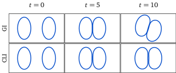
Figure 3: Snapshots of two vesicles in extensional flow using GI and CLI schemes. As the distance between two vesicles decreases the configuration loses symmetry in the GI scheme as shown in the top row. Nevertheless, as shown in the second row, the LI with minimal-separation constraint scheme maintains the desired minimum separation distance and two vesicles also maintain a symmetric configuration. (The viscosity contrast is 500 in this simulation).

In Fig. 4(a), we plot the minimal distance between two vesicles over time. The vesicles continue to get closer in the GI scheme. However, the CLI scheme maintains the desired minimum separation distance between two vesicles. In Fig. 4(b), we show the minimum distance between the vesicles over the course of simulation (with time horizon $T=10$) versus the viscosity contrast. As expected, we observe that the minimum distance between two vesicles decreases as the viscosity contrast is increased. Consequently, for higher viscosity contrast with both GI and LI schemes, either the configuration loses its symmetry or the two vesicles intersect. With minimal-separation constraint, we any desired minimum separation distance between vesicles is maintained, and the simulation is more robust and accurate as shown in Fig. 3 and Table 2.

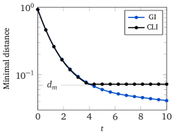
((a)) The minimal distance of two vesicles over time

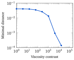
((b)) The minimum distance between two vesicles versus the viscosity contrast

Figure 4: Distance between two vesicles in extensional flow. LABEL:sub@sfg:exten-dis-time The minimum distance between two vesicles over time for both CLI and GI schemes. The CLI scheme easily maintains the prescribed minimal separation of $h$. LABEL:sub@sfg:exten-dis-visc The final distance (at $T=10$) between two vesicles as viscosity contrast is increased in GI scheme.

$\nu$	$\Delta t$	CLI	LI	GI
$1$	$0.4$	$1.17e{-01}$	$1.17e{-01}$	$7.66e{-02}$
$1$	$0.2$	$9.49e{-04}$	$9.49e{-04}$	$1.03e{-03}$
$1$	$0.1$	$4.49e{-04}$	$4.49e{-04}$	$4.69e{-04}$
$1$	$0.05$	$2.23e{-04}$	$2.23e{-04}$	$2.29e{-04}$
$1$	$0.025$	$1.12e{-04}$	$1.12e{-04}$	$1.14e{-04}$
$1$	$0.0125$	$5.65e{-05}$	$5.65e{-05}$	$5.68e{-05}$
$1e2$	$0.4$	$9.42e{-03}$	$-$	$2.54e{-04}$
$1e2$	$0.2$	$1.33e{-04}$	$1.33e{-04}$	$1.22e{-04}$
$1e2$	$0.1$	$6.38e{-05}$	$6.38e{-05}$	$5.96e{-05}$
$1e2$	$0.05$	$3.05e{-05}$	$3.05e{-05}$	$2.95e{-05}$
$1e2$	$0.025$	$1.49e{-05}$	$1.49e{-05}$	$1.47e{-05}$
$1e2$	$0.0125$	$7.39e{-06}$	$7.39e{-05}$	$7.32e{-06}$

$\nu$	$\Delta t$	CLI	LI	GI
$1e3$	$0.4$	$8.88e{-03}^{T=8.8}$	$-$	$1.66e{-05}$
$1e3$	$0.2$	$2.08e{-02}$	$-$	$7.99e{-06}$
$1e3$	$0.1$	$5.85e{-06}$	$-$	$3.93e{-06}$
$1e3$	$0.05$	$2.42e{-06}$	$1.93e{-06}$	$1.95e{-06}$
$1e3$	$0.025$	$1.12e{-06}$	$9.78e{-07}$	$7.33e{-07}$
$1e3$	$0.0125$	$5.89e{-07}$	$4.87e{-07}$	$2.01e{-07}$
$1e4$	$0.4$	$1.45e{-03}^{T=3.6}$	$-$	$-$
$1e4$	$0.2$	$7.23e{-04}^{T=5.4}$	$-$	$-$
$1e4$	$0.1$	$7.75e{-04}^{T=6.8}$	$-$	$-$
$1e4$	$0.05$	$2.41e{-06}$	$-$	$-$
$1e4$	$0.025$	$1.17e{-06}$	$-$	$-$
$1e4$	$0.0125$	$5.58e{-07}$	$-$	$-$

Table 2: Error in the length of vesicles in extensional flow. The error in the final length of two vesicles in extensional flow with respect to viscosity contrast, timestep size, and for different schemes. The experiment’s setup is described in Section 4.1 and snapshots of which are shown in Fig. 3. The cases with a “$-$” indicate that either vesicles have intersected or the GMRES failed to converge due to ill-conditioning of the system; the latter happens in the GI scheme and high viscosity contrast. Cases with superscript indicate that the flow loses its symmetry at that time.

In Table 2, we report the final error in vesicle perimeter for different schemes with respect to viscosity contrast and timestep size. With minimal-separation constraint, we achieve similar or smaller error in length compared to LI or GI methods (when these methods produce a valid result). Moreover, one can use relatively large time step in all flow parameters—most notably when vesicles have high viscosity contrast. In contrast, the LI scheme requires very small, often impractical, time steps to prevent instability or intersection.

4.2 Shear flow

We consider vesicles and rigid bodies in an unbounded shear flow and explore the effects of minimal separation on shear diffusivity. In the first simulation, we consider two vesicles of reduced area $0.98$ (to minimize the effect of vesicles’ relative orientation on the dynamics) placed in a shear flow with shear rate $\chi=2$. Let $\delta_{t}=|y_{t}^{1}-y_{t}^{2}|$ denote the vertical offset between the centroids of vesicles at time $t$. Initially, two vesicles are placed with a relative vertical offset $\delta_{0}$ as show in Fig. 5.

((a)) $t=5$

((b)) $t=7.5$

((c)) $t=10$

((d)) $t=12$

Figure 5: Shear flow experiment setup. The snapshots of two vesicles in shear flow. Initially, one vesicle is placed at $[-8,\delta_{0}]$ and the second vesicle is placed at $[0,0]$.

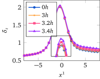
((a)) Centroid trajectory (vesicle)

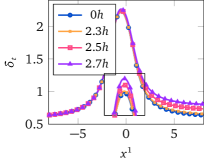
((b)) Centroid trajectory (rigid)

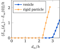
((c)) Final centroid offset

Figure 6: The offset $\delta_{t}(d_{m})$ between the centroids of two vesicles in shear flow. The initial offset is $\delta_{0}=0.64$ and $N=64$ discretization points are used, implying $h=0.0994$, where $h$ is the distance between two discretization points along vesicle boundary. LABEL:sub@sfg:shear-cm and LABEL:sub@sfg:shear-cmrgd show $\delta_{t}(x^{1})$ for the vesicles and circular rigid particles for different minimal separation distance $d_{m}$. LABEL:sub@sfg:shear-sd shows the excess displacement induced by minimal separation. When collision constraint is activate (larger $d_{m}$), the particles are in effect hydrodynamically larger and the excess displacement grows linearly with $d_{m}$.

In Fig. 6, we report $\delta_{t}$ and its value upon termination of the simulation when $x^{1}>8$, denoted by $\delta_{\infty}(d_{m})$. In Figs. 6(a) and 6(b), we plot $\delta_{t}$ with respect to the $x^{1}$ for different minimum separation distances. Based on a high-resolution simulation (with $N=128$ and $8\times$ smaller time step), the minimal distance between two vesicles without contact constraint is about $2.9h$ for vesicles and $2.2h$ for rigid particles. As the minimum separation parameter $d_{m}$ is decreased below this threshold, the simulations with minimal-separation constraint converge to the reference simulation without minimal-separation constraint. In Fig. 6(c), we plot the excess terminal displacement due to contact constraint, $(\delta_{\infty}(d)-\delta_{\infty}(0))/h$, as a function of the minimum separation distance. When collision constraint is activate, the particles are in effect hydrodynamically larger and the excess displacement grows linearly with $d_{m}$.

4.3 Sedimentation

To compare the performance of schemes with and without contact constraints, we first consider a small problem with three vesicles sedimenting in a container. We compare three first-order time stepping schemes: locally implicit (LI), locally implicit with collision handling (CLI), and globally implicit (GI).

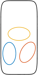
((a)) CLI $t=0$

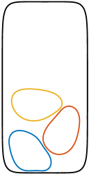
((b)) CLI $t=5$

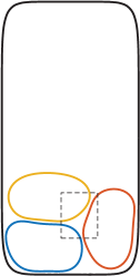
((c)) CLI $t=20$

((d)) CLI $t=20$

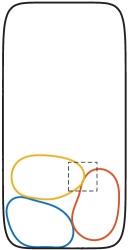
((e)) GI $t=10$

((f)) GI $t=10$

Figure 7: Sedimenting vesicles. Snapshots of three sedimenting vesicles in a container using three time-stepping schemes. The vesicles have reduced area of $0.9$, their viscosity contrast is $100$, and are discretized with $64$ points. The boundary is discretized with $256$ points, the simulation time horizon $T=26$, and the time step is $0.01$. LABEL:sub@sfg:sed3nv-snap1–LABEL:sub@sfg:sed3nv-snap3 The dynamics of three vesicles sedimenting with CLI scheme. LABEL:sub@sfg:sed3nv-snap3z The contact region of LABEL:sub@sfg:sed3nv-snap3. LABEL:sub@sfg:sed3nv-impcol The instance when the vesicles intersect using GI scheme. LABEL:sub@sfg:sed3nv-impcolz The contact region of LABEL:sub@sfg:sed3nv-impcol.

Snapshots of these simulations are shown in Fig. 7. For the LI scheme, the error grows rapidly when the vesicles intersect and a $64\times$ smaller time step is required for resolving the contact and for stability. Similarly, for the GI scheme the vesicle intersect as shown in Figs. 7(e) and 7(f) and a $4\times$ smaller time step is needed for the contact to be resolved. The CLI scheme, maintains the desired minimal separation between vesicles.

Although the current code is not optimized for computational efficiency, it is instructive to consider the relative amount of time spent for a single time step in each scheme. Each time step in LI scheme takes about $1$ second, the time goes up to $1.5$ seconds for the CLI scheme. In contrast, a single time step with the GI scheme takes, on average, $65$ seconds because the solver needs up to 240 GMRES iterations to converge when vesicles are very close. This excessive cost renders this scheme impractical for large problems.

To demonstrate the capabilities of the CLI scheme and to gain a qualitative understanding of the scaling of the cost as the number of intersections increases, we consider the sedimentation of $100$ vesicles. As the sediment progresses the number of contact regions grows to about $70$ per time step. For this simulation, we use a lower viscosity contrast of $10$ and the enclosing boundary is discretized with $512$ points and the total time is $T=30$. Snapshots of the simulation with CLI scheme are shown in Fig. 1.

We observe that with first-order time stepping, both LI and CLI schemes are unstable. Therefore, we run this simulation with second order SDC using LI and CLI schemes. The GI scheme is prohibitively expensive and infeasible in this case, due to ill-conditioning and large number of GMRES iterations per time-step.

The LI scheme requires at least $12000$ thousand time steps to maintain the non-intersection constraint and each time step takes about $700$ seconds to complete. On the other hand, the CLI scheme only need $1500$ time steps to complete the simulation (taking the stable time step) and each time step takes about $830$ seconds. We repeated this experiment with $16$ discretization points on each vesicle using CLI scheme and $1500$ time steps are also sufficient for this case (with final length error about $3.83e{-3}$), each time step takes about $170$ seconds and the simulation takes about $70$ hours to complete. The number of contact resolving iterations in Algorithm 1 is about $10$.

In summary, LI scheme requires $4\times$ more points on each vesicle and $8\times$ smaller time-step size to keep vesicles in a valid configuration compared to CLI scheme.

4.4 Convergence analysis

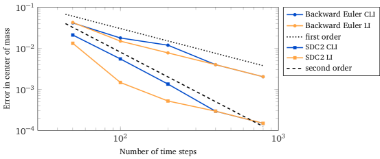
Figure 8: Convergence rate. We compare the final center of mass of three sedimenting vesicles in a container for Backward Euler and SDC2 (second order Spectral Deferred Correction scheme). The time horizon is set to $T=2$. We choose the spatial resolution proportional to the time-step. As a reference, we use the results for the GI scheme with time step $\Delta t=1.25e{-3}$ and $N=256$ discretization points on each vesicle and $512$ discretization points on the boundary.

To investigate the accuracy of the time-stepping schemes, we consider the sedimentation of three vesicles with reduced area $0.9$ in a container as shown in Fig. 7. We test LI and CLI schemes for a range of time steps and spatial resolutions and report the error in the location of the center of mass of the vesicles at the end of simulation. The spatial resolution $h$ is chosen proportional to time-step size and for the CLI scheme the minimal separation $d_{m}$ is proportional to $h$. As a reference, we use a fine-resolution simulation with GI scheme. The error as a function of time step size is shown in Fig. 8.

4.5 Stenosis

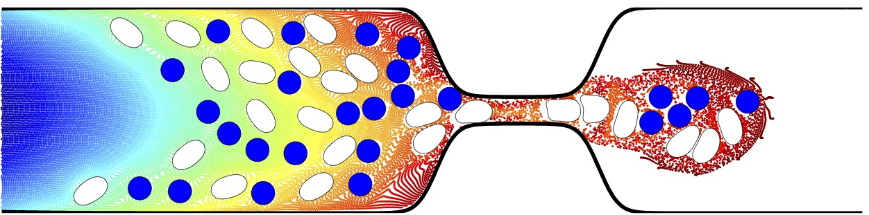
((b)) $t=4.5$

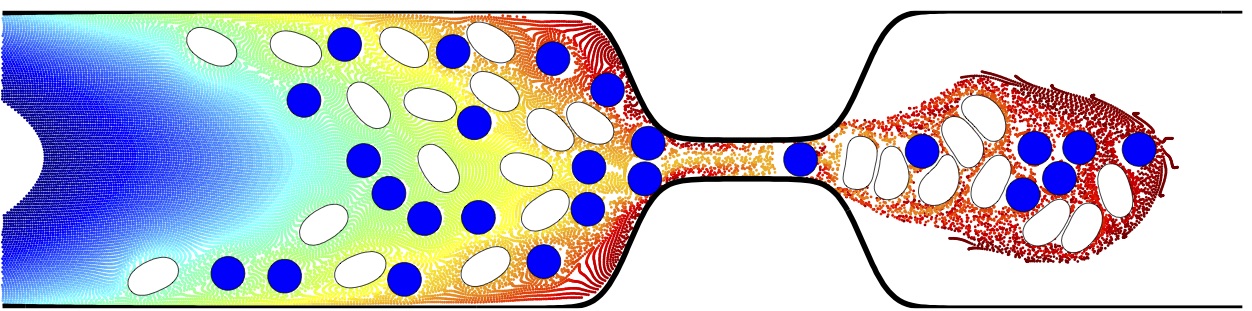
((c)) $t=6.1$

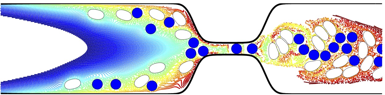
((d)) $t=11.3$

Figure 9: Stenosis with $25$ vesicles and $25$ rigid particles. Snapshots of vesicles and rigid particles passing a constricted tube, the fluid flows from left to right (using proper Dirichlet boundary condition on the wall). The colored tracers are for visualization purposes and do not induce any flow. The simulation time horizon is set to $T=20$, each vesicle or rigid particle is discretized with $32$ points, and the wall is discretized with $1024$ points. LABEL:sub@sfg:choke-snap1 The initial configuration. LABEL:sub@sfg:choke-snap2–LABEL:sub@sfg:choke-snap4 The interaction and collision between vesicles, rigid particles, and the domain boundary at different instances. Without minimal-separation constraint, vesicles and rigid particles easily contact at the entrance of the constricted area.

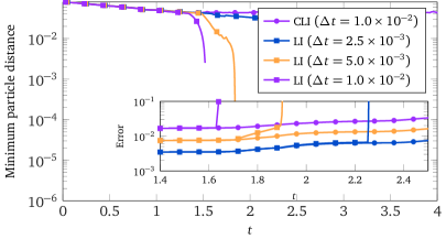
Figure 10: error for stenosis example. The minimal distance and error for different schemes and time step sizes. For the $LI$ scheme, independently of the time step size, vesicles or particles intersect with the domain boundary, resulting in divergence. The CLI scheme is stable and maintains the desired minimal distance.

As a stress test for particle-boundary and vesicle-boundary interaction, we study the flow with $25$ vesicles of reduced area $0.9$, mixed with $25$ circular rigid particles in a constricted tube (Section 1.4). It is well known that rigid bodies can become arbitrarily close in the Stokes flow, e.g. [29], and without proper collision handling, the required temporal/spatial resolution would be very high.

In this example, the vesicles and rigid particles are placed at the right hand side of the constricted tube. We use backward Euler method and search for the stable time step for schemes LI and CLI. Similarly to the sedimentation example, we do not consider the $GI$ scheme due to its excessive computational cost.

The largest stable time step for the CLI scheme is $\Delta t=0.01$. For the LI scheme, we tested the cases with up to $32\times$ smaller time step size, but we were unable to avoid contact and intersection between vesicles and rigid particles.

Figure 10 shows the error and minimal distance between vesicles, particles, and boundary for CLI and LI schemes with different time step sizes. Without the minimal-separation constraint, the solution diverges when the particles cross the domain boundary.

To validate our estimates for the errors due to using a piecewise-linear approximation in the minimal separation constraint instead of high-order shapes, we plot the minimum distance at each step for the piecewise-linear approximation and upsampled shapes in Fig. 11. The target minimal separation distance is set to $d_{m}=h$. We observe that the actual minimal distance for smooth curve is smaller than the minimal distance for piecewise-linear curve, while the difference between two distances is small compared to the target minimum separation distance.

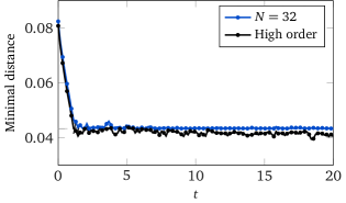
Figure 11: Effective minimal distance. The minimal distance between 32-point piecewise-linear approximations (enforced by the constraint) and the true minimal distance between high-order shapes. We use an upsampled linear approximation with $N=128$ as the surrogate for the high-order curves.

Note that the due to higher shear rate in the constricted area, the stable time step is dictated by the dynamics in that area. For such flows, we expect a combination of adaptive time stepping [49] and the scheme outlined in this paper provide the highest speedup.

5 Conclusion

In this paper we introduced a new scheme for efficient simulation of dense suspensions of deformable and rigid particles immersed in Stokesian fluid. We demonstrated through numerical experiments that this scheme is orders of magnitude faster than the alternatives and can achieve high order temporal accuracy. We are working on extending this approach to three dimensions and using adaptive time stepping.

We extend our thanks to George Biros, David Harmon, Ehssan Nazockdast, Bryan Quaife, Michael Shelley, and Etienne Vouga for stimulating conversations about various aspects of this work.

References

- [1] BH Ahn “Solution of nonsymmetric linear complementarity problems by iterative methods” In Journal of Optimization Theory and Applications 33.2, 1981, pp. 175–185
- [2] Jérémie Allard, François Faure, Hadrien Courtecuisse, Florent Falipou, Christian Duriez and Paul G. Kry “Volume contact constraints at arbitrary resolution” In ACM SIGGRAPH 2010 papers on - SIGGRAPH ’10 C, 2010, pp. 1
- [3] Bradley K Alpert “Hybrid Gauss-trapezoidal quadrature rules” In SIAM Journal on Scientific Computing 20.5, 1999, pp. 1551–1584
- [4] Uri M Ascher, Steven J Ruuth and Brian TR Wetton “Implicit-Explicit methods for time-dependent partial differential equations” In SIAM Journal on Numerical Analysis 32.3 SIAM, 1995, pp. 797–823
- [5] David Baraff and Andrew Witkin “Large steps in cloth simulation” In Proceedings of the 25th annual conference on Computer graphics and interactive techniques - SIGGRAPH ’98, 1998, pp. 43–54
- [6] Himanish Basu, Aditya K. Dharmadhikari, Jayashree A. Dharmadhikari, Shobhona Sharma and Deepak Mathur “Tank treading of optically trapped red blood cells in shear flow” In Biophysical Journal 101.7, 2011, pp. 1604 –1612
- [7] A. R. Bausch and K. Kroy “A bottom-up approach to cell mechanics” In Nature Physics 2.4, 2006, pp. 231–238
- [8] Thierry Biben, Klaus Kassner and Chaouqi Misbah “Phase-field approach to three-dimensional vesicle dynamics” In Physical Review E 72.4, 2005, pp. 041921
- [9] Richard W Cottle, Jong-Shi Pang and Richard E Stone “The linear complementarity problem” SIAM, 2009
- [10] Qiang Du and Jian Zhang “Adaptive finite element method for a phase field bending elasticity model of vesicle membrane deformations” In SIAM Journal on Scientific Computing 30.3, 2008, pp. 1634–1657
- [11] Christian Duriez, Frédéric Dubois, Abderrahmane Kheddar and Claude Andriot “Realistic haptic rendering of interacting deformable objects in virtual environments.” In IEEE transactions on visualization and computer graphics 12.1, 2006, pp. 36–47
- [12] Ch Eck, O Steinbach and WL Wendland “A symmetric boundary element method for contact problems with friction” In Mathematics and Computers in Simulation 50.1, 1999, pp. 43–61
- [13] Kenny Erleben “Numerical methods for linear complementarity problems in physics-based animation” In ACM SIGGRAPH 2013 Courses, 2013
- [14] Alexander Farutin, Thierry Biben and Chaouqi Misbah “3D Numerical simulations of vesicle and inextensible capsule dynamics”, 2013
- [15] François Faure, Sébastien Barbier, Jérémie Allard and Florent Falipou “Image-based collision detection and response between arbitrary volume objects” In Proceedings of the 2008 ACM i, 2008, pp. 155–162
- [16] KA Fischer and P Wriggers “Frictionless 2D contact formulations for finite deformations based on the mortar method” In Computational Mechanics 36.3, 2005, pp. 226–244
- [17] JB Freund “Leukocyte margination in a model microvessel” In Physics of Fluids (1994-present) 19.2, 2007, pp. 023301
- [18] J. M. Frostad, J. Walter and L. G. Leal “A scaling relation for the capillary-pressure driven drainage of thin films” In Physics of Fluids 25.5, 2013, pp. 052108
- [19] G. Ghigliotti, A. Rahimian, G. Biros and C. Misbah “Vesicle migration and spatial organization driven by flow line curvature” In Physical Review Letters 106.2, 2011, pp. 028101
- [20] H Gun “Boundary element analysis of 3-D elasto-plastic contact problems with friction” In Computers & structures 82.7, 2004, pp. 555–566
- [21] David Harmon, Etienne Vouga, Rasmus Tamstorf and Eitan Grinspun “Robust treatment of simultaneous collisions” In ACM SIGGRAPH 2008 papers on - SIGGRAPH ’08, 2008, pp. 1
- [22] David Harmon, Etienne Vouga, Breannan Smith, Rasmus Tamstorf and Eitan Grinspun “Asynchronous contact mechanics” In ACM Transactions on Graphics 28.3, 2009, pp. 1
- [23] David Harmon, Daniele Panozzo, Olga Sorkine and Denis Zorin “Interference-aware geometric modeling” In ACM Transactions on Graphics 30.6, 2011, pp. 1
- [24] Kenneth Langstreth Johnson and Kenneth Langstreth Johnson “Contact mechanics” Cambridge university press, 1987
- [25] Yongsam Kim and Ming-Chih Lai “Simulating the dynamics of inextensible vesicles by the penalty immersed boundary method” In Journal of Computational Physics 229.12, 2010, pp. 4840–4853
- [26] Rolf H Krause and Barbara I Wohlmuth “A Dirichlet–Neumann type algorithm for contact problems with friction” In Computing and visualization in science 5.3, 2002, pp. 139–148
- [27] Aymen Laadhari, Pierre Saramito and Chaouqi Misbah “Computing the dynamics of biomembranes by combining conservative level set and adaptive finite element methods” In Journal of Computational Physics 263, 2014, pp. 328–352
- [28] Carlton E Lemke “Bimatrix equilibrium points and mathematical programming” In Management science 11.7, 1965, pp. 681–689
- [29] M. Loewenberg and EJ J. Hinch “Collision of two deformable drops in shear flow” In Journal of Fluid Mechanics 338, 1997, pp. 299–315
- [30] Michael Loewenberg “Numerical simulation of concentrated emulsion flows” In Journal of Fluids Engineering 120.4, 1998, pp. 824
- [31] OL Mangasarian “Solution of symmetric linear complementarity problems by iterative methods” In Journal of Optimization Theory and Applications 22.4, 1977, pp. 465–485
- [32] Chaouqi Misbah “Vacillating breathing and tumbling of vesicles under shear flow” In Physical Review Letters 96, 2006, pp. 028104
- [33] Ehssan Nazockdast, Abtin Rahimian, Denis Zorin and Michael Shelley “Fast and high-order methods for simulating fiber suspensions applied to cellular mechanics” preprint, 2015
- [34] M. Nemer, X. Chen, D. Papadopoulos, J. Bławzdziewicz and M. Loewenberg “Hindered and enhanced coalescence of drops in stokes flows” In Physical Review Letters 92.11, 2004, pp. 114501
- [35] Jorge Nocedal and Stephen Wright “Numerical optimization” Springer Science & Business Media, 2006
- [36] Hiroshi Noguchi and Gerhard Gompper “Vesicle dynamics in shear and capillary flows” In Journal of Physics: Condensed Matter 17.45, 2005, pp. S3439–S3444
- [37] Rikard Ojala and Anna-Karin Tornberg “An accurate integral equation method for simulating multi-phase Stokes flow”, 2014, pp. 1–22
- [38] Miguel a. Otaduy, Rasmus Tamstorf, Denis Steinemann and Markus Gross “Implicit contact handling for deformable objects” In Computer Graphics Forum 28.2, 2009, pp. 559–568
- [39] H Power “The completed double layer boundary integral equation method for two-dimensional Stokes flow” In IMA Journal of Applied Mathematics, 1993
- [40] Henry Power and Guillermo Miranda “Second kind integral equation formulation of Stokes’ flows past a particle of arbitrary shape” In SIAM Journal on Applied Mathematics 47.4, 1987, pp. 689
- [41] C. Pozrikidis “The axisymmetric deformation of a red blood cell in uniaxial straining Stokes flow” In Journal of Fluid Mechanics 216, 1990, pp. 231–254
- [42] C. Pozrikidis “Boundary integral and singularity methods for linearized viscous flow”, Cambridge Texts in Applied Mathematics Cambridge University Press, Cambridge, 1992
- [43] C Pozrikidis “Dynamic simulation of the flow of suspensions of two-dimensional particles with arbitrary shapes” In Engineering Analysis with Boundary Elements 25.1, 2001, pp. 19–30
- [44] Xavier Provot “Collision and self-collision handling in cloth model dedicated to design garments” In Computer Animation and Simulation’97, 1997
- [45] Michael A Puso “A 3D mortar method for solid mechanics” In International Journal for Numerical Methods in Engineering 59.3, 2004, pp. 315–336
- [46] Michael A Puso, TA Laursen and Jerome Solberg “A segment-to-segment mortar contact method for quadratic elements and large deformations” In Computer Methods in Applied Mechanics and Engineering 197.6, 2008, pp. 555–566
- [47] Bryan Quaife and George Biros “High-volume fraction simulations of two-dimensional vesicle suspensions” In Journal of Computational Physics 274, 2014, pp. 245–267
- [48] Bryan Quaife and George Biros “High-order adaptive time stepping for vesicle suspensions with viscosity contrast” In Procedia IUTAM 16, 2015, pp. 89–98
- [49] Bryan Quaife and George Biros “Adaptive time stepping for vesicle suspensions” In Journal of Computational Physics 306, 2016, pp. 478–499
- [50] Abtin Rahimian, Shravan Kumar Veerapaneni and George Biros “Dynamic simulation of locally inextensible vesicles suspended in an arbitrary two-dimensional domain, a boundary integral method” In Journal of Computational Physics 229.18, 2010, pp. 6466–6484
- [51] Abtin Rahimian, Shravan K. Veerapaneni, Denis Zorin and George Biros “Boundary integral method for the flow of vesicles with viscosity contrast in three dimensions” In Journal of Computational Physics 298, 2015, pp. 766–786
- [52] J.M. Rallison and A. Acrivos “A numerical study of the deformation and burst of a viscous drop in an extensional flow” In Journal of Fluid Mechanics 89, 1978, pp. 191–200
- [53] E. Sackmann “Supported membranes: Scientific and practical applications” In Science 271, 1996, pp. 43–48
- [54] Ashok S Sangani and Guobiao Mo “Inclusion of lubrication forces in dynamic simulations” In Physics of Fluids 6.5, 1994, pp. 1653–1662
- [55] Jin Sun Sohn, Yu-Hau Tseng, Shuwang Li, Axel Voigt and John S Lowengrub “Dynamics of multicomponent vesicles in a viscous fluid” In Journal of Computational Physics 229.1, 2010, pp. 119–144
- [56] S Sukumaran and Udo Seifert “Influence of shear flow on vesicles near a wall: a numerical study” In Physical Review E 64.1, 2001, pp. 011916
- [57] M Tur, FJ Fuenmayor and P Wriggers “A mortar-based frictional contact formulation for large deformations using Lagrange multipliers” In Computer Methods in Applied Mechanics and Engineering 198.37, 2009, pp. 2860–2873
- [58] Shravan K. Veerapaneni, Denis Gueyffier, Denis Zorin and George Biros “A boundary integral method for simulating the dynamics of inextensible vesicles suspended in a viscous fluid in 2D” In Journal of Computational Physics 228.7, 2009, pp. 2334–2353
- [59] Peter Wriggers “Finite element algorithms for contact problems” In Archives of Computational Methods in Engineering 2.4, 1995, pp. 1–49
- [60] Peter Wriggers “Computational contact mechanics” Springer Science & Business Media, 2006
- [61] Alireza Yazdani and Prosenjit Bagchi “Three-dimensional numerical simulation of vesicle dynamics using a front-tracking method” In Physical Review E 85.5, 2012, pp. 056308
- [62] G. K. Youngren and A. Acrivos “Stokes flow past a particle of arbitrary shape: a numerical method of solution” In Journal of Fluid Mechanics 69, 1975, pp. 377–403
- [63] Hong Zhao and Eric S. G. Shaqfeh “The dynamics of a vesicle in simple shear flow” In Journal of Fluid Mechanics 674, 2011, pp. 578–604
- [64] Hong Zhao and Eric S. G. Shaqfeh “The dynamics of a non-dilute vesicle suspension in a simple shear flow” In Journal of Fluid Mechanics 725, 2013, pp. 709–731
- [65] Hong Zhao, Amir H.G. Isfahani, Luke N. Olson and Jonathan B. Freund “A spectral boundary integral method for flowing blood cells” In Journal of Computational Physics 229.10, 2010, pp. 3726–3744
- [66] Hua Zhou and C. Pozrikidis “The flow of ordered and random suspensions of two-dimensional drops in a channel” In Journal of Fluid Mechanics 255, 1993, pp. 103–127
- [67] Alexander Z. Zinchenko and Robert H. Davis “A boundary-integral study of a drop squeezing through interparticle constrictions” In Journal of Fluid Mechanics 564, 2006, pp. 227
- [68] Alexander Z. Zinchenko, MA Michael A. Rother and RH Robert H. Davis “A novel boundary-integral algorithm for viscous interaction of deformable drops” In Physics of Fluids 9.6, 1997, pp. 1493