Non-minimal Coupling of Torsion-matter Satisfying Null Energy Condition for Wormhole Solutions

Abstract

We explore wormhole solutions in a non-minimal torsion-matter coupled gravity by taking an explicit non-minimal coupling between the matter Lagrangian density and an arbitrary function of torsion scalar. This coupling depicts the transfer of energy and momentum between matter and torsion scalar terms. The violation of null energy condition occurred through effective energy-momentum tensor incorporating the torsion-matter non-minimal coupling while normal matter is responsible for supporting the respective wormhole geometries. We consider energy density in the form of non-monotonically decreasing function along with two types of models. First model is analogous to curvature-matter coupling scenario, that is, torsion scalar with $T$-matter coupling while the second one involves a quadratic torsion term. In both cases, we obtain wormhole solutions satisfying null energy condition. Also, we find that the increasing value of coupling constant minimizes or vanishes the violation of null energy condition through matter.

Keywords: Wormhole; Non-minimal coupling; Torsion; $f(T)$ gravity; Energy conditions.
PACS: 04.50.kd; 95.35.+d; 02.40.Gh.

1 Introduction

The topological handles which connect distant regions of the universe as a bridge or tunnel is named as wormhole. The most amazing thing is the two-way travel through wormhole tunnel which happened when throat remains open. That is, to prevent the wormhole from collapse at non-zero minimum value of radial coordinate. In order to keep the throat open, the exotic matter is used which violate the null energy condition and elaborated the wormhole trajectories as hypothetical paths. The violation of null energy condition is the basic ingredient to integrate wormhole solutions. This configuration is firstly studied by Flamm [1] and then leads Einstein and Rosen [2] to contribute into the successive steps for the construction of wormhole solutions. The work of Morris and Thorne [3] evoked the wormhole scenario and leads to the new directions. The usual matter are considered to satisfy the energy conditions, therefore, some exotic type matter is employed for these solutions. There exists some wormhole solutions in semi-classical gravity through quantum effects such as Hawking evaporation and Casimir effects [3, 4] where energy conditions are violated. One may take some such types of matter which acted as exotic matter, for instance, phantom energy [5], tachyon matter [6], generalized Chaplygin gas [7], some non-minimal kinetic coupling, etc.

In order to find some realistic sources that support the wormhole geometry or minimize the usage of exotic matter, different variety of wormhole solutions are explored. This includes thin-shell, dynamical and rotating wormholes [8]. However, the concentration goes towards modified theories of gravity where the effective scenario gives the violation of null energy condition and matter source supports the wormholes. Bronnikov and Starobinsky [9] proved a general no-go theorem which yields no wormholes (static or dynamic) can be constituted in any ghost-free scalar-tensor theory of gravity (which also includes $f(R)$ gravity as a particular case), under some conditions on the non-minimal coupling function. In $f(R)$ gravity, Lobo and Oliveira [10] found that the higher curvature terms in effective energy-momentum tensor are responsible for the necessary violation for the wormhole solutions in ghost-containing scenario. They assumed a particular shape function along with various fluids to check the validity of energy conditions. Jamil et al. [11] discussed several static wormhole solutions in this gravity with a noncommutative geometry background through Gaussian distribution. They considered power-law solution as first and construct wormhole geometry as well as analyzed the validity of energy conditions. Secondly, they explored these solutions with the help of shape function. Taking into account Lorentzian distribution of energy density, Rahaman et al. [12] derived some new exact solutions under same manner and gave some viable wormhole solutions.

In extended teleparallel gravity being the modification of teleparallel gravity [13, 14], static as well as dynamical wormhole solutions are also explored. In this way, Böhmer et al. [15] investigated wormhole solutions in this gravity by taking some specific $f(T)$ forms, shape function as well as redshift functions which are the basic characteristics of these solutions. Assuming different fluids such as baro-tropic, isotropic and anisotropic, Jamil et al. [16] enquired the possibility of some realistic sources for wormhole solutions. Sharif and Rani explored the wormhole solutions in this gravity taking noncommutative background with Gaussian distribution [17], dynamical wormhole solutions [18], for the traceless fluid [19], with the inclusion of charge [20] and galactic halo scenario [21]. They considered some power-law $f(T)$ functions for which effective energy-momentum tensor depending on torsion contributed terms violated the null energy condition. Recently, Jawad and Rani [22] constructed wormhole solutions via Lorentzian distribution in noncommutative background. They concluded that their exist the possibility of some realistic wormhole solutions satisfying energy conditions and stayed in equilibrium. We also studied some higher dimensional wormhole solutions in Einstein Gauss-Bonnet gravity [23].

The modification of theories taking some non-minimal coupling between matter and curvature becomes center of interest now-a-days. There exist such theories involving these coupling as $f(R)=f_{1}(R)+[1+\lambda f_{2}(R)]\mathcal{L}_{m}$ and $f(R,\mathcal{L}_{m})$, [24] etc. Harko et al. [25] introduced the most general conditions in the framework of modified gravity, that is the matter threading the wormhole throat satisfies all of the energy conditions while the gravitational fluid (such as higher order curvature terms) support the nonstandard wormhole geometries. They explicitly showed that wormhole geometries can be theoretically constructed without the presence of exotic matter but are sustained in the context of modified gravity. Taking into account some specific cases of modified theories of gravity, namely, $f(R)$ gravity, the curvature-matter coupling and the $f(R,\mathcal{L}_{m})$ generalization, they showed explicitly that one may choose the parameters of the theory such that the matter threading the wormhole throat satisfies the energy conditions.

Following the same scenario as for $f(R)$ theory, Harko et al. [26] proposed non-minimal torsion-matter coupling as a extension of $f(T)$ gravity. In this gravity, two arbitrary functions $f_{1}(T)$ and $f_{2}(T)$ are introduced such as $f_{1}$ is the extension of geometric part while $f_{2}$ is coupled with matter Lagrangian part through some coupling constant. They discussed this theory for cosmological aspects of evolving universe and deduced that the universe may represent quintessence, phantom or crossing of phantom-divide line, inflationary era, de Sitter accelerating phase, in short, a unified description. In this gravity, Nashed [27], Feng et al. [28] and Carloni et al. [29] studied spherically symmetric solutions, cosmological evolutions and compared their results with observational data and phase space analysis, respectively. Garcia and Lobo [30] explored wormhole solutions by non-minimal curvature-matter coupling taking linear functions, $f_{1}=R,~{}f_{2}=R$. They concluded that the wormhole solutions in realistic manner depends on higher values of coupling parameter.

The paper has following symmetry. In next section 2, we describe the $f(T)$ gravity and non-minimal torsion-matter coupling extension. Section 3 is devoted to the gravitational field equations for wormhole geometry in the coupling scenario. We find the general conditions on matter part for the validity of null energy condition. Also, we examined the effective energy-momentum tensor being the responsible for violation of null energy condition. In section 4, we explore wormhole solutions taking into account two well-known models. These models involving linear torsion scalar coupled with $T$-matter and quadratic torsion term with matter represented wormhole geometry. In the last section, we summarize the results.

2 Non-minimal Torsion-matter Coupling

In this section, we mainly review the torsion based gravitational paradigm. The torsional scenario begins with a spacetime undergoing the absolute parallelism where the parallel vector field ${h_{\beta}}^{a}$ determines

$${\Gamma^{a}}_{bc}={h_{\beta}}^{a}{h^{\beta}}_{b,c},$$ (1)

which is a non-symmetric affine connection with vanishing curvature and $h_{\beta a,b}=\partial_{b}h_{\beta a}$. Here we apply the Latin indices as the notation for tangent spacetime while coordinate spacetime indices are presented with the help of Greek letters. The parallel vector fields (vierbein or tetrad fields) are the basic dynamical variables which deduce an orthonormal basis for the tangent space, i.e., $\textbf{h}_{a}\cdot\textbf{h}_{b}=\eta_{ab}$ where $\eta=\textmd{diag}(1,-1,-1,-1)$. In terms of vierbein components, ${h^{\beta}}_{a}$, the vierbein fields are defined as $\textbf{h}_{a}={h^{\beta}}_{a}\partial_{\beta}$ while the inverse components ${h_{a}}^{\beta}$ meet the following conditions

$${h^{a}}_{\beta}{h_{b}}^{\beta}=\delta^{a}_{b},\quad{h_{a}}^{\beta}{h^{a}}_{\alpha}=\delta^{\beta}_{\alpha}.$$

The metric tensor is obtained through the relation $g_{\beta\alpha}=\eta_{ab}{h^{a}}_{\beta}{h^{b}}_{\alpha}$ which gives the metric determinant as $\sqrt{-g}=e=\textmd{det}({h^{a}}_{\beta})$. Using Eq.(1), the antisymmetric part of Weitzenböck connection yields

$${T^{\beta}}_{\alpha\sigma}={\widetilde{\Gamma}^{\beta}}_{~{}\sigma\alpha}-{\widetilde{\Gamma}^{\beta}}_{~{}\alpha\sigma}={h_{a}}^{\beta}(\partial_{\sigma}{h^{a}}_{\alpha}-\partial_{\alpha}{h^{a}}_{\sigma}),$$ (2)

where ${T^{\beta}}_{\alpha\gamma}=-{T^{\beta}}_{\gamma\alpha}$, i.e., it is antisymmetric in its lower indices. It is noted that the under the parallel transportation of vierbein field, the curvature of the Weitzenböck connection vanishes. Using this tensor, we obtain contorsion tensor as $K^{\alpha\gamma}_{~{}~{}\beta}=-\frac{1}{2}(T^{\alpha\gamma}_{~{}~{}\beta}-T^{\gamma\alpha}_{~{}~{}\beta}-T_{\beta}^{~{}\alpha\gamma})$ and superpotential tensor as ${S_{\beta}}^{\alpha\gamma}=\frac{1}{2}[\delta^{\alpha}_{\beta}{T^{\mu\gamma}}_{\mu}-\delta^{\gamma}_{\beta}{T^{\mu\alpha}}_{\mu}+K^{\alpha\gamma}_{~{}~{}\beta}]$. The torsion scalar takes the form

$$T={S_{\beta}}^{\alpha\gamma}{T^{\beta}}_{\alpha\gamma}.$$ (3)

The action of $f(T)$ gravity is given by [13, 14]

$$\mathcal{S}=\frac{1}{16\pi\mathcal{G}}\int e\{f(T)+\mathcal{L}_{m}\}d^{4}x.$$ (4)

The $\mathcal{G}$ is the gravitational constant and $f$ represents the generic differentiable function of torsion scalar describing extension of the teleparallel gravity. The term $\mathcal{L}_{m}$ describes the matter part of the action such as $\mathcal{L}_{m}=\mathcal{L}_{m}(\rho,~{}p)$ where $\rho,~{}p$ are the energy density and pressure of matter while we neglect the radiation section for the sake of simplicity. By the variation of this action w.r.t vierbein field, the following field equations come out

$${h_{a}}^{\beta}{S_{\beta}}^{\alpha\sigma}\partial_{\alpha}Tf_{{}_{TT}}+[{h_{a}}^{\beta}{T^{\lambda}}_{\alpha\beta}{S_{\lambda}}^{\sigma\alpha}+\frac{1}{e}\partial_{\alpha}(h{h_{a}}^{\beta}{S_{\beta}}^{\alpha\sigma})]f_{{}_{T}}+\frac{1}{4}{h_{a}}^{\sigma}f=4\pi\mathcal{G}{h_{a}}^{\beta}\Theta^{\sigma}_{\beta},$$ (5)

where the subscripts involving $T$ and $TT$ represent first and second order derivatives of $f$ with respect to $T$ respectively. For the sake of simplicity, we assume $8\pi\mathcal{G}=1$ in the following.

The $f(T)$ field equations in terms of Einstein tensor gain a remarkable importance in order to discuss various cosmological and astrophysical scenarios [13, 14]. This type of field equations take place by replacing partial derivatives to covariant derivatives along with compatibility of metric tensor, i.e., $\nabla_{\sigma}g_{\beta\alpha}=0$. Using the relations $T^{\mu(\nu\gamma)}=K^{(\mu\nu)\gamma}=S^{\mu(\nu\gamma)}=0$, the torsion, contorsion and superpotential tensor become

$${T^{\sigma}}_{\beta\alpha}=h^{\sigma}_{a}(\nabla_{\beta}h^{a}_{\alpha}-\nabla_{\alpha}h^{a}_{\beta}),\quad{K^{\sigma}}_{\beta\alpha}=h^{\sigma}_{a}\nabla_{\alpha}h^{a}_{\beta},$$

$${S_{\sigma}}^{\alpha\beta}=\eta^{ab}h^{\beta}_{a}\nabla_{\sigma}h^{\alpha}_{b}+\delta^{\alpha}_{\sigma}\eta^{ab}h^{\tau}_{a}\nabla_{\tau}h^{\beta}_{b}-\delta^{\beta}_{\sigma}\eta^{ab}h^{\tau}_{a}\nabla_{\tau}h^{\alpha}_{b}.$$

The curvature tensor referred to Weitzenböck connection vanishes, while the Riemann tensor related with the Levi-Civita connection ${\Gamma^{\gamma}}_{\mu\nu}$ is given by

$${R^{\sigma}}_{\beta\lambda\alpha}=\nabla_{\alpha}{K^{\sigma}}_{\beta\lambda}-\nabla_{\lambda}{K^{\sigma}}_{\beta\alpha}+{K^{\sigma}}_{\tau\alpha}{K^{\tau}}_{\beta\lambda}-{K^{\sigma}}_{\tau\lambda}{K^{\tau}}_{\beta\alpha}.$$

We obtain the Ricci tensor and scalar as follows

$$R_{\beta\alpha}=-\nabla^{\sigma}S_{\alpha\sigma\beta}-g_{\beta\alpha}\nabla^{\sigma}{T^{\lambda}}_{\sigma\lambda}-{S^{\sigma\lambda}}_{\beta}K_{\lambda\sigma\alpha},\quad R+T=-2\nabla^{\sigma}{T^{\alpha}}_{\sigma\alpha},$$ (6)

where we use ${S^{\alpha}}_{\sigma\alpha}=-2{T^{\alpha}}_{\sigma\alpha}=2{K^{\alpha}}_{\sigma\alpha}$. Substituting Eq.(6) along with Einstein tensor $G_{\beta\alpha}=R_{\beta\alpha}-\frac{1}{2}g_{\beta\alpha}R$, we get

$$G_{\beta\alpha}-\frac{1}{2}g_{\beta\alpha}T=-\nabla^{\sigma}S_{\alpha\sigma\beta}-{S^{\tau\sigma}}_{\beta}K_{\sigma\tau\alpha},$$ (7)

Finally, inserting this equation in Eq.(5), it yields

$$f_{T}G_{\beta\alpha}+\frac{1}{2}g_{\beta\alpha}(f-Tf_{T})+Z_{\beta\alpha}f_{TT}=\Theta_{\beta\alpha},$$ (8)

where $Z_{\beta\alpha}={S_{\alpha\beta}}^{\sigma}\nabla_{\sigma}T$. This equation expresses a similar structure like $f(R)$ gravity at least up to equation level and representing GR for the limit $f(T)=T$. We take trace of the above equation, i.e., $Zf_{TT}-(R+2T)f_{T}+2f=\Theta$, with $Z={Z^{\alpha}}_{\alpha}$ and $\Theta={\Theta^{\alpha}}_{\alpha}$ to simplify the field equations. The $f(T)$ field equations can be rewritten as

$$G_{\beta\alpha}=\frac{1}{f_{{}_{T}}}\big{[}\Theta_{\beta\alpha}^{m}-Z_{\beta\alpha}f_{{}_{TT}}-\frac{1}{2}(f-Tf_{{}_{T}})\big{]},$$ (9)

where $\Theta_{\beta\alpha}^{m}$ is the energy-momentum tensor corresponding to matter Lagrangian.

Taking into account non-minimal coupling between torsion and matter, Harko et al. [26] defined the action as follows

$$\mathcal{S}=\int e\{f_{1}+(1+\omega f_{2})\mathcal{L}_{m}\}d^{4}x,$$ (10)

where $\omega$ is the coupling constant having units of mass^-2 and $f_{1},~{}f_{2}$ are arbitrary differential functions of torsion scalar. Applying the tetrad variation on this action, we obtain the following set of equations

$${h_{a}}^{\beta}{S_{\beta}}^{\alpha\sigma}\partial_{\alpha}T(f^{\prime\prime}_{1}+\omega f^{\prime\prime}_{2}\mathcal{L}_{m})+[{h_{a}}^{\beta}{T^{\lambda}}_{\alpha\beta}{S_{\lambda}}^{\sigma\alpha}+\frac{1}{e}\partial_{\alpha}(h{h_{a}}^{\beta}{S_{\beta}}^{\alpha\sigma})](f^{\prime}_{1}+\omega f^{\prime}_{2}\mathcal{L}_{m})$$

$$+\frac{1}{4}{h_{a}}^{\sigma}f_{1}-\frac{1}{4}\omega\partial_{\alpha}T{h_{a}}^{\beta}{\mathcal{T}^{\sigma\alpha}_{\beta}}f^{\prime}_{2}+\omega f^{\prime}_{2}{h_{a}}^{\beta}{S_{\beta}}^{\sigma\alpha}\partial_{\alpha}\mathcal{L}_{m}=\frac{1}{2}(1+\omega f_{2}){h_{a}}^{\beta}\Theta^{\sigma}_{\beta},$$ (11)

where the number of primes denotes the correspondingly order derivative with respect to torsion scalar and ${\mathcal{T}^{\sigma\alpha}_{a}}=\frac{\partial\mathcal{L}_{m}}{\partial\partial_{\alpha}{h^{a}}_{\sigma}}$. We assume here that the matter Lagrangian $\mathcal{L}_{m}$ is independent of derivatives of tetrad which results the vanishing of ${\mathcal{T}^{\sigma\alpha}_{a}}$. Also, the Bianchi identities of teleparallel gravity express the following relationship

$$\nabla_{\beta}\Theta_{\tau}^{\beta}=\frac{4}{1+\omega f_{2}}{K^{\lambda}}_{\beta\tau}{S_{\lambda}}^{\beta\alpha}\nabla_{\alpha}(f^{\prime}_{1}+\omega f^{\prime}_{2}\mathcal{L}_{m})-\frac{\omega f^{\prime}_{2}}{1+\omega f_{2}}(\Theta^{\beta}_{\tau}-\mathcal{L}_{m}\delta^{\beta}_{\tau})\nabla_{\beta}T.$$ (12)

This equation represents the substitute of energy and momentum between torsion and matter through defined coupling. The $f(T)$ field equations for the torsion-matter coupling in the form of Einstein tensor are given by

$$G_{\beta\alpha}=\frac{1}{f_{{}_{1T}}+\omega f_{{}_{2T}}\mathcal{L}_{m}}\bigg{[}\Theta_{\beta\alpha}^{+}-{S_{\alpha\beta}}^{\lambda}\nabla_{\lambda}(f_{{}_{1TT}}+\omega f_{{}_{2TT}}\mathcal{L}_{m})-\mathcal{J}g_{{}_{\beta\alpha}}\bigg{]},$$ (13)

where

$$\mathcal{J}=\frac{1}{2}\bigg{\{}f_{1}-T(f_{{}_{1T}}+\omega f_{{}_{2T}}\mathcal{L}_{m})\bigg{\}},\quad\Theta_{\beta\alpha}^{+}=(1+\omega f_{2})\Theta_{\beta\alpha}^{m}-\omega f_{{}_{2T}}{S_{\alpha\beta}}^{\lambda}\nabla_{\lambda}\mathcal{L}_{m}.$$

It is noted that the matter Lagrangian density needs to be properly defined in the analysis of torsion-matter coupling. In the literature for curvature-matter coupling, the proposals for this matter Lagrangian density are as follows [30].
(i)  $\mathcal{L}_{m}=p$ which reproduce the equation of state for perfect fluid and proved as not unique.
(ii)  $\mathcal{L}_{m}=-ne$ where $e$ denotes physical free energy defined by $e=-\mathbb{T}s+\frac{\rho}{n},~{}\mathbb{T}$ is the temperature, $s$ being the entropy of one particle and $n$ gives the particle number density.
(iii)  $\mathcal{L}_{m}=-\rho$ representing a natural choice which gives the energy in a local rest frame for the fluid.

3 Gravitational Field Equations for Wormhole Geometry

In order to construct the gravitational field equations in the framework of torsion-matter coupling, we firstly describe the wormhole geometry. Let us assume the wormhole metric as follows [17]-[23]

$$ds^{2}=e^{2\Psi(r)}dt^{2}-\frac{1}{1-\frac{b}{r}}dr^{2}-r^{2}d\phi^{2}-r^{2}\sin^{2}\phi d\psi^{2},$$ (14)

where redshift function $\Psi$ and shape function $b$ are $r$ dependent functions. In order to set geometry of wormhole scenario, some constraints are required on both of these functions. These are describe as follows.

• Shape function: The shape of the wormhole consists of two open mouths (two asymptomatically flat regions) in different regions of the space connected through throat which is minimum non-zero value of radial coordinate. This shape maintains through the shape function $b(r)$ with increasing behavior and having ratio $1$ with $r$. At throat, it must holds $b(r_{0})=r_{0}$ as well as $1-\frac{b(r)}{r}\geq 0$. The flare-out condition being the fundamental property of wormhole geometry is defined as

  $$\frac{1}{b^{2}}(b-b^{\prime}r)>0.$$ (15)

  There is another constraint on the derivative of shape function at throat, i.e., $b^{\prime}(r_{0})<1$ which must be fulfilled.

• Redshift function: The main purpose of wormholes is to give a way to move two-way through its tunnel which basically depends on non-zero minimum value of $r$ at throat. For this purpose, i.e., to keep throat open, the redshift function plays its role by maintaining no-horizon at throat. To hold this condition, $\Psi$ must remains finite throughout the spacetime. This function calculates the gravitational redshift of a light particle. When this particle moves from potential well to escape to infinity, there appears a reduction in its frequency which is called gravitational redshift. At a particular value of $r$, its infinitely negative value expresses an event horizon at throat. To prevent this situation of appearing horizon so that wormhole solution may provide traversable way, the magnitude of its redshift function must be finite. This may be taken as $\Psi=0$ which gives $e^{2\Psi(r)}\rightarrow 1$.

• Exotic matter: The existence of wormhole solutions requires some unusual type of matter, called exotic matter having negative pressure to violate the null energy condition. Thus, it becomes the basic factor for wormhole construction as the known classical forms of matter satisfy this condition. The search for such a source which provides the necessary violation with matter content obeying the null energy condition occupy a vast range of study in astrophysics.

The energy conditions originates through the Raychaudhuri equation in the realm of general relativity for the expansion regarding positivity of the term $R_{\beta\alpha}\mathcal{K}^{\beta}\mathcal{K}^{\alpha}$ where $\mathcal{K}^{\beta}$ denotes the null vector. This positivity guarantees a finite value of the parameter marking points on the geodesics directed by geodesic congruences. In terms of energy-momentum tensor, the above term under positivity condition become $R_{\beta\alpha}\mathcal{K}^{\beta}\mathcal{K}^{\alpha}=\Theta_{\beta\alpha}\mathcal{K}^{\beta}\mathcal{K}^{\alpha}\geq 0$ in the framework of general relativity. However, in modified theories of gravity, we carry effective energy-momentum tensor which is further used in the above expression to study energy conditions. For instance, in the underlying case, Eq.(13) takes the form

$$G_{\beta\alpha}=\Theta^{\textmd{eff}}_{\beta\alpha},\quad\textmd{where}\quad\Theta^{\textmd{eff}}_{\beta\alpha}=\frac{1}{f_{{}_{1T}}+\omega f_{{}_{2T}}\mathcal{L}_{m}}[\Theta_{\beta\alpha}^{+}+\Theta_{\beta\alpha}^{\textmd{TM}}],$$ (16)

where $\Theta_{\beta\alpha}^{\textmd{TM}}=-{S_{\alpha\beta}}^{\lambda}\nabla_{\lambda}(f_{{}_{1TT}}+\omega f_{{}_{2TT}}\mathcal{L}_{m})-\mathcal{J}g_{{}_{\beta\alpha}}$ representing contribution of torsion-matter coupling in the extended teleparallel gravity. The corresponding energy condition becomes $R_{\beta\alpha}\mathcal{K}^{\beta}\mathcal{K}^{\alpha}=\Theta^{\textmd{eff}}_{\beta\alpha}\mathcal{K}^{\beta}\mathcal{K}^{\alpha}\geq 0$ which is called null energy condition. Taking into account perfect fluid with presentation $\Theta_{\beta\alpha}=(\rho^{\textmd{eff}}+p^{\textmd{eff}})\mathcal{U}_{\beta}\mathcal{U}_{\alpha}-p^{\textmd{eff}}g_{\beta\alpha}$, this condition yields $\rho^{\textmd{eff}}+p^{\textmd{eff}}\geq 0$.

At this stage, we may impose a condition on energy-momentum tensor corresponding to matter part such that $\Theta^{m}_{\beta\alpha}\mathcal{K}^{\beta}\mathcal{K}^{\alpha}\geq 0$ to thread the wormhole while $\Theta^{\textmd{eff}}_{\beta\alpha}\mathcal{K}^{\beta}\mathcal{K}^{\alpha}\leq 0$ gives the necessary violation. This condition implies the positivity of energy density in all local frames of references. Thus, it is important to study the constraints on $\Theta^{m}_{\beta\alpha}$ in order to form wormholes. Consider the violation of null energy condition and Eq.(16), we get

$$\frac{1}{f_{{}_{1T}}+\omega f_{{}_{2T}}\mathcal{L}_{m}}\bigg{[}(1+\omega f_{2})\Theta_{\beta\alpha}^{m}-\omega f_{{}_{2T}}{S_{\alpha\beta}}^{\lambda}\nabla_{\lambda}\mathcal{L}_{m}-{S_{\alpha\beta}}^{\lambda}\nabla_{\lambda}(f_{{}_{1TT}}$$

$$+\omega f_{{}_{2TT}}\mathcal{L}_{m})-\mathcal{J}g_{{}_{\beta\alpha}}\bigg{]}\mathcal{K}^{\beta}\mathcal{K}^{\alpha}<0.$$

For the viable wormhole solutions, if $(f_{{}_{1T}}+\omega f_{{}_{2T}}\mathcal{L}_{m})>0$, then we obtain the following constraint

$$0\leq\Theta_{\beta\alpha}^{m}\mathcal{K}^{\beta}\mathcal{K}^{\alpha}<\frac{1}{1+\omega f_{2}}\bigg{[}\omega f_{{}_{2T}}{S_{\alpha\beta}}^{\lambda}\nabla_{\lambda}\mathcal{L}_{m}+{S_{\alpha\beta}}^{\lambda}\nabla_{\lambda}(f_{{}_{1TT}}$$

$$+\omega f_{{}_{2TT}}\mathcal{L}_{m})+\mathcal{J}g_{{}_{\beta\alpha}}\bigg{]}\mathcal{K}^{\beta}\mathcal{K}^{\alpha},$$

where $1+\omega f_{2}>0$ must holds. For the case $(f_{{}_{1T}}+\omega f_{{}_{2T}}\mathcal{L}_{m})<0$, the null energy condition straightforwardly gives

$$\Theta_{\beta\alpha}^{m}\mathcal{K}^{\beta}\mathcal{K}^{\alpha}>\frac{1}{1+\omega f_{2}}\bigg{[}\omega f_{{}_{2T}}{S_{\alpha\beta}}^{\lambda}\nabla_{\lambda}\mathcal{L}_{m}+{S_{\alpha\beta}}^{\lambda}\nabla_{\lambda}(f_{{}_{1TT}}$$

$$+\omega f_{{}_{2TT}}\mathcal{L}_{m})+\mathcal{J}g_{{}_{\beta\alpha}}\bigg{]}\mathcal{K}^{\beta}\mathcal{K}^{\alpha}.$$

We consider the case $\mathcal{L}_{m}=-\rho$ with no horizon condition, that is $\Psi=0$ to construct the background geometry for wormhole solutions in the framework of $f(T)$ gravity having torsion-matter coupling. We take anisotropic distribution of fluid having energy-momentum tensor as

$$\Theta_{\beta\alpha}^{m}=(\rho+p_{r})\mathcal{U}_{\beta}\mathcal{U}_{\alpha}-p_{r}g_{\beta\alpha}+(p_{t}-p_{r})\chi_{\beta}\chi_{\alpha},$$ (17)

where $p_{r}$ is the radial directed pressure component and $p_{t}$ denotes tangential pressure component with $\rho=\rho(r),~{}p=p(r)$ satisfying $\mathcal{U}^{\beta}\mathcal{U}_{\alpha}=-\chi^{\beta}\chi_{\alpha}=1$. Taking into account Eqs.(13) and (14), we obtain a set of field equations as follows

$$\frac{b^{\prime}}{r^{2}} = \frac{1}{f_{{}_{1T}}-\omega f_{{}_{2T}}\rho}\bigg{[}(1+\omega f_{2})\rho+\frac{\omega f_{{}_{2T}}\rho^{\prime}}{r}\bigg{(}1-\frac{b}{r}-\sqrt{1-\frac{b}{r}}\bigg{)}\bigg{]}$$ (18)

$$- \frac{T^{\prime}(f_{{}_{1TT}}-\omega f_{{}_{2TT}}\rho)}{r(f_{{}_{1T}}-\omega f_{{}_{2T}}\rho)}\bigg{(}1-\frac{b}{r}-\sqrt{1-\frac{b}{r}}\bigg{)}-\frac{\mathcal{J}}{f_{{}_{1T}}-\omega f_{{}_{2T}}\rho},$$

$$-\frac{b}{r^{3}} = \frac{(1+\omega f_{2})p_{r}}{f_{{}_{1T}}-\omega f_{{}_{2T}}\rho}+\frac{\mathcal{J}}{f_{{}_{1T}}-\omega f_{{}_{2T}}\rho},$$ (19)

$$-\frac{b^{\prime}r-b}{2r^{3}} = \frac{1}{f_{{}_{1T}}-\omega f_{{}_{2T}}\rho}\bigg{[}(1+\omega f_{2})p_{t}-\frac{\omega f_{{}_{2T}}\rho^{\prime}}{2r}\bigg{(}1-\frac{b}{r}-\sqrt{1-\frac{b}{r}}\bigg{)}\bigg{]}$$ (20)

$$+ \frac{T^{\prime}(f_{{}_{1TT}}-\omega f_{{}_{2TT}}\rho)}{2r(f_{{}_{1T}}-\omega f_{{}_{2T}}\rho)}\bigg{(}1-\frac{b}{r}-\sqrt{1-\frac{b}{r}}\bigg{)}+\frac{\mathcal{J}}{f_{{}_{1T}}-\omega f_{{}_{2T}}\rho},$$

where prime represents derivative with respect to $r$ and

$$T=\frac{2}{r^{2}}\bigg{[}2\bigg{(}1-\sqrt{1-\frac{b}{r}}\bigg{)}-\frac{b}{r}\bigg{]}.$$ (21)

The violation of null energy condition $(\Theta^{\textmd{eff}}_{\beta\alpha}\mathcal{K}^{\beta}\mathcal{K}^{\alpha}<0)$ for field equations (18)-(20) is checked through the consideration of radial null vector which yields

$$\rho^{\textmd{eff}}+p_{r}^{\textmd{eff}} = \frac{1}{f_{{}_{1T}}-\omega f_{{}_{2T}}\rho}\bigg{[}(1+\omega f_{2})(\rho+p_{r})+\frac{1}{r}\bigg{\{}\omega f_{{}_{2T}}\rho^{\prime}$$

$$- T^{\prime}(f_{{}_{1TT}}-\omega f_{{}_{2TT}}\rho)\bigg{\}}\bigg{(}1-\frac{b}{r}-\sqrt{1-\frac{b}{r}}\bigg{)}\bigg{]}$$

$$= \frac{b^{\prime}r-b}{r^{3}}<0,$$

$$\Rightarrow\rho^{\textmd{eff}}+p_{r}^{\textmd{eff}} < 0,$$

where the inequality comes through the flaring out condition of shape function. In order to discuss the above scenario at throat, we obtain the following relationship

$$\rho^{\textmd{eff}}(r_{0})+p_{r}^{\textmd{eff}}(r_{0}) = \frac{1}{f_{{}_{1T_{0}}}-\omega f_{{}_{2T_{0}}}\rho_{0}}\bigg{[}(1+\omega f_{2}(r_{0}))(\rho_{0}+p_{r0})+\frac{1}{r_{0}}\bigg{\{}\omega f_{{}_{2T_{0}}}\rho_{0}^{\prime}$$

$$- T^{\prime}_{0}(f_{{}_{1T_{0}T_{0}}}-\omega f_{{}_{2T_{0}T_{0}}}\rho_{0})\bigg{\}}\bigg{(}1-\frac{b_{0}}{r_{0}}-\sqrt{1-\frac{b_{0}}{r_{0}}}\bigg{)}\bigg{]},$$

which must satisfy the following constraint in order to meet the above inequality, that is

$$(1+\omega f_{2}(r_{0}))(\rho_{0}+p_{r0})+\frac{1}{r_{0}}\omega f_{{}_{2T_{0}}}\rho_{0}^{\prime}\bigg{(}1-\frac{b_{0}}{r_{0}}-\sqrt{1-\frac{b_{0}}{r_{0}}}\bigg{)}<$$

$$\frac{T^{\prime}_{0}}{r_{0}}(f_{{}_{1T_{0}T_{0}}}-\omega f_{{}_{2T_{0}T_{0}}}\rho_{0})\bigg{(}1-\frac{b_{0}}{r_{0}}-\sqrt{1-\frac{b_{0}}{r_{0}}}\bigg{)},$$

where $f_{{}_{1T_{0}}}-\omega f_{{}_{2T_{0}}}\rho_{0}>0$ while the inequality reverses if $f_{{}_{1T_{0}}}-\omega f_{{}_{2T_{0}}}\rho_{0}<0$. In order to write final field equations in terms of matter component, we observe that the last term in all Eqs.(18)-(20) change its sign using signature (-,+,+,+) for wormhole spacetime while remaining terms stay same. This leads to the vanishing of last terms in each equation as energy density is independent of signature. Finally, the field equations can be rewritten as

$$b^{\prime}\big{(}f_{{}_{1T}}-\omega f_{{}_{2T}}\rho\big{)} = r^{2}(1+\omega f_{2})\rho+\omega\bigg{[}\omega f_{{}_{2T}}\rho^{\prime}-T^{\prime}(f_{{}_{1TT}}-\omega f_{{}_{2TT}}\rho)\bigg{]}$$ (22)

$$\times \bigg{(}1-\frac{b}{r}-\sqrt{1-\frac{b}{r}}\bigg{)},$$

$$p_{r} = -\frac{b}{r^{3}}\frac{f_{{}_{1T}}-\omega f_{{}_{2T}}\rho}{1+\omega f_{2}},$$ (23)

$$p_{t} = \frac{1}{2r(1+\omega f_{2})}\bigg{[}\bigg{(}f_{{}_{1T}}-\omega f_{{}_{2T}}\rho\bigg{)}\bigg{(}\frac{b}{r^{2}}-\frac{b^{\prime}}{r}\bigg{)}-\bigg{\{}\omega\rho^{\prime}f_{{}_{2T}}$$ (24)

$$+ T^{\prime}(f_{{}_{1TT}}-\omega f_{{}_{2TT}}\rho)\bigg{\}}\bigg{(}1-\frac{b}{r}-\sqrt{1-\frac{b}{r}}\bigg{)}\bigg{]}.$$

4 Wormhole Solutions

In order to discuss wormhole solutions, we have to deal with un-closed system of equations such that the three equations with $f_{1},~{}f_{2},~{}\rho,~{}p_{r},~{}p_{t}$ and $b$ are unknown functions. Due to non-linear appearance of these equations, the explicit functions are extremely difficult. However, we may adopt some alternative strategies keeping in mind the characteristics of wormhole geometry. To involve the effects of non-minimal torsion-matter coupling to construct the wormhole solutions, we have to choose some viable models $f_{1}$ and $f_{2}$. Now we are remaining with four unknowns for which we may assume some kind of equation of state like equation obeying the traceless fluid, particular value of shape function obeying all corresponding conditions or some type of energy density like density of static spherically symmetric smearing object, etc. We adopt the last approach of considering energy density with particular form [30]

$$\rho=\rho_{0}\bigg{(}\frac{r_{0}}{r}\bigg{)}^{\sigma},$$ (25)

where $\rho_{0}$ and $\sigma$ are positive constants.

In the following, we consider two viable $f(T)$ models and study the different conditions of shape functions as well as null energy condition.

4.1 Model 1

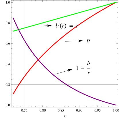
Figure 1: Plots of shape function $b,~{}1-\frac{b}{r},~{}b=r~{}\textmd{versus}~{}r$ for Model 1 using $r_{0}=1,~{}\rho_{0}=0.75,~{}\sigma=3$ and $\omega=0.4$.

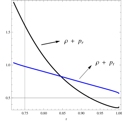
Figure 2: Plots of null energy condition $\rho+p_{r},~{}\rho+p_{t}~{}\textmd{versus}~{}r$ for Model 1 using $r_{0}=1,~{}\rho_{0}=0.75,~{}\sigma=3$ and $\omega=0.4$.

Figure 3: The general relativistic deviation profile versus $\omega$ for Model 1 using $r_{0}=1,~{}\rho_{0}=0.75$ and $\sigma=3$.

As a first model, we consider the models $f_{1}=T$ and $f_{2}=T$ analogous to the case of curvature-matter coupling scenario where these models are taken as $f_{1}=R=f_{2}$ [30]. Substituting these values of models along with Eq.(25) in (22), we obtain the following differential equation for the shape function

$$b^{\prime}-\frac{\omega\sigma\rho_{0}\big{(}\frac{r_{0}}{r}\big{)}^{\sigma}}{1-\omega\rho_{0}\big{(}\frac{r_{0}}{r}\big{)}^{\sigma}}\bigg{(}\frac{b}{r}+\sqrt{1-\frac{b}{r}}\bigg{)}=-\frac{\sigma\rho_{0}\big{(}\frac{r_{0}}{r}\big{)}^{\sigma}}{1-\omega\rho_{0}\big{(}\frac{r_{0}}{r}\big{)}^{\sigma}}[r(1+\omega T)+\omega].$$ (26)

We plot the shape function by numerically in order to study the wormhole geometry as shown in Figure 1 fixing initial condition as $b(1)=1$. We take some particular values of constants as $r_{0}=1,~{}\rho_{0}=0.75,~{}\omega=0.4$ and plot versus $r$. The plot of $b$ represents positively increasing behavior with respect to $r$. The trajectory of $1-\frac{b}{r}$ depicts the positive behavior for $r\leq 1$ which meets the condition $b<r$. Figure 2 shows the null energy condition taking both components of pressure along with chosen energy density. The black curve represents $\rho+p_{r}$ and blue curve describes $\rho+p_{t}$ versus $r$ taking into account Eqs.(23)-(25). We see that the null energy condition holds in this case. Thus the possibility of wormhole solutions for which the normal matter satisfying the null energy condition in the background of torsion-matter coupling exists.

Figure 3 represents the general relativistic deviation profile of null energy condition for radial pressure component which gives the range of coupling parameter. At throat, the null energy condition implies

$$(\rho+p_{r})\mid_{r=r_{0}}=\rho_{0}-\frac{1-\omega\rho_{0}}{r_{0}^{2}+2\omega}.$$

For the chosen values of parameters, we obtain the range of coupling constant as $\omega\geq 0.11$ for which null energy condition holds. This depicts that the increasing value of coupling constant minimizes or vanishes the violation of null energy condition through matter. For the case when there is no coupling, i.e., $\omega=0$, Eq.(22) reduces to $b^{\prime}=-\sigma\rho_{0}r_{0}^{\sigma}r^{1-\sigma}$. The solution of this equation is $b=-\frac{\sigma\rho_{0}r_{0}^{\sigma}}{2-\sigma}r^{2-\sigma}+c$, where $c$ is an integration constant and can be determined by $b(r_{0})=r_{0}$. After applying this condition, finally the shape function becomes

$$b(r)=r_{0}\bigg{(}1+\frac{\sigma\rho_{0}r_{0}}{2-\sigma}\bigg{)}-\frac{\sigma\rho_{0}r_{0}^{\sigma}}{2-\sigma}r^{2-\sigma}.$$

This shape function shows a asymptomatically flat geometry as $\frac{b}{r}\rightarrow 0$ as $r\rightarrow\infty$. Taking same values of parameters, this function gives $b=-1.25+\frac{2.25}{r}$ representing decreasing but positive behavior for $r<1.8$ while $1-\frac{b}{r}$ holds for two sets of ranges $(r>-2.25~{}\textmd{and}~{}r>1)$ or $(r<-2.25~{}\textmd{and}~{}r<1)$. Also, the condition $b^{\prime}(r_{0})<1$ meets as $b^{\prime}=-\sigma\rho_{0}r_{0}<1$. The expression $\rho+p_{r}=\frac{1}{r^{4}}(2r-2.25)$ leads to $r>1.125$ to meet the null energy condition while $\rho+p_{t}=\frac{1}{2r^{4}}(0.25r+4.5)$ which remains positive.

4.2 Model 2

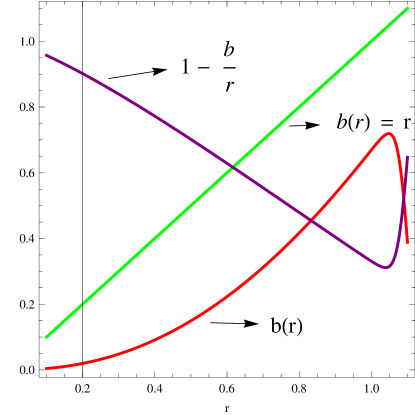
Figure 4: Plots of shape function $b,~{}1-\frac{b}{r},~{}b=r~{}\textmd{versus}~{}r$ for Model 2 using $r_{0}=1,~{}\rho_{0}=0.75,~{}\sigma=3,~{}\mu=0.2,~{}\nu=-2$ and $\omega=0.4$.

As the second choice for the model, we consider the viable model with quadratic torsion term as [26]

$$f_{1}=-\Lambda,~{}\quad f_{2}=\mu T+\nu T^{2},$$ (27)

where $\Lambda>0,~{}\mu$ and $\nu$ are constants. This model describes a well-depicted result in cosmological scenario, i.e., a matter-dominated phase followed by phantom phase of the universe. Substituting Eqs.(25) and (27) in (22), we obtain the following differential equation

$$b^{\prime}+\frac{r}{\mu+2\nu T}\bigg{\{}\frac{\sigma(\mu+2\nu T)}{r}-2\nu T^{\prime}\bigg{\}}\bigg{(}\frac{b}{r} + \sqrt{1-\frac{b}{r}}-1\bigg{)}=-\frac{r^{2}}{1+\omega(\mu+2\nu T)}$$ (28)

$$\times \bigg{(}1+\omega(\mu+\nu T)T\bigg{)}.$$

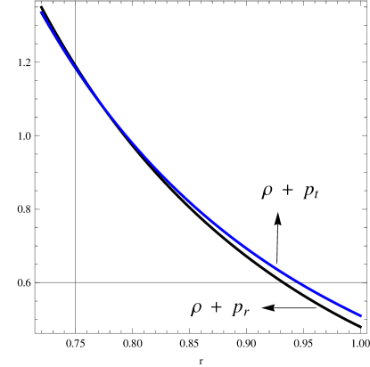
Figure 5: Plots of null energy condition $\rho+p_{r},~{}\rho+p_{t}~{}\textmd{versus}~{}r$ for Model 2 using $r_{0}=1,~{}\rho_{0}=0.75,~{}\sigma=3,~{}\mu=0.2,~{}\nu=-2$ and $\omega=0.4$.

Figure 6: The general relativistic deviation profile versus $\omega$ for Model 2 using $r_{0}=1,~{}\rho_{0}=0.75,~{}\sigma=3,~{}\mu=0.2,~{}\nu=-2$.

Figure 4 represents the plots of shape function under different conditions through numerical computations. The trajectory of $b$ describes positively increasing behavior for $r\geq 1$ and then decreasing behavior. The plot of $1-\frac{b}{r}$ respects positive behavior. Thus, for model 2, we obtain wormhole geometry for torsion-matter coupling. The null energy condition for this model is plotted in Figure 5 which shows the positivity of the condition. In order to check the relativistic deviation profile taking into account null energy condition for radial pressure component at throat, we find the equation as follows

$$(\rho+p_{r})\mid_{r=r_{0}}=\rho_{0}+\frac{\omega(\mu r_{0}^{2}+4\nu)\rho_{0}}{r_{0}^{4}+2\omega(\mu r_{0}^{2}+2\nu)}.$$

Its plot is shown in Figure 6 representing $\omega>0.15$ for the range where null energy condition holds. This depicts that the increasing value of coupling constant minimizes or vanishes the violation of null energy condition through matter. Also, we may discuss the case of zero coupling in the similar way as discussed for Model 1.

5 Concluding Remarks

The search for wormhole solutions satisfying energy conditions becomes the most interesting configuration now-a-days. Wormhole is a tube like shape or tunnel which is assumed to be a source to link distant regions in the universe. The most amazing thing is the two-way travel through wormhole tunnel which happened when throat remains open. That is, to prevent the wormhole from collapse at non-zero minimum value of radial coordinate. In order to keep the throat open, the exotic matter is used which violate the null energy condition and elaborated the wormhole trajectories as hypothetical paths. In order to find some realistic sources which support the wormhole geometry, the concentration is goes towards modified theories of gravity. In these theories, effective scenario gives the violation of null energy condition and matter source supports the wormholes. In this paper, the wormhole geometries are explored taking a non-minimal coupling between torsion and matter part in extended teleparallel gravity. This coupling expresses the exchange of energy and momentum between both parts torsion and matter.

The extension of $f(T)$ gravity appeared in terms of two arbitrary functions $f_{1}(T)$ and $f_{2}(T)$ where $f_{1}$ is the extension of geometric part while $f_{2}$ is coupled with matter Lagrangian part through some coupling constant. At throat, the general conditions imposed by the null energy condition taking energy-momentum tensor of matter Lagrangian are presented in terms of non-minimal torsion-matter coupling. The field equations appeared in non-linear form which are difficult to solve for analytical solutions. Presented various strategies to solve these equations, we have adopted to assume two viable models with a non-monotonically decreasing function of energy density. These models involving linear torsion scalar coupled with $T$-matter and quadratic torsion term with matter represented wormhole geometry. For these solutions, the null energy condition is satisfied. It is concluded that that the null energy condition is satisfied for increasing values of coupling constant. This depicted that, the usage of exotic matter can be reduced or vanished with the higher values of coupling constant. Thus through the torsion-matter coupling, we have obtained some wormhole solutions in realistic way such that matter source satisfied the energy conditions while effective part having torsion-matter coupled terms provided the necessary violation. Finally, we remark here that this work may be a useful contribution for the present theory as well as astrophysical aspects.

References

- [1] Flamm, L.: Phys. Z. 17(1916)448.
- [2] Einstein, A. and Rosen, N.: Phys. Rev. 48(1935)73.
- [3] Morris, M.S. and Thorne, K.S.: Am. J. Phys. 56395(1988).
- [4] Thorne, M.S., Thorne, K.S. and Yurtsever, U.: Phys. Rev. Lett. 61(1988)1446.
- [5] Lobo, F.S.N.: Phys. Rev. D 71(2005)084011; Sushkov, S.V.: Phys. Rev. D 71(2005)043520; Sharif, M. and Jawad, A.: Eur. Phys. J. Plus 129(2014)15.
- [6] Das, A. and Kar, S.: Class. Quantum Gravit. 22(2005)3045.
- [7] Lobo, F.S.N.: Phys. Rev. D 73(2006)064028.
- [8] Garcia, N.M., Lobo, F.S.N. and Visser, M.: Phys. Rev. D 86(2012)044026; Richarte, M.G. and Simeone, C.: Phys. Rev. D 76(2007)087502; Teo, E.: Phys. Rev. D 58(1998)024014; Kashargin, P.E. and Sushkov, S.V.: Phys. Rev. D 78(2008)064071; Kar, S. and Sahdev, D.: Phys. Rev. D 53(1996)722; Arellano, A.V.B. and Lobo, F.S.N.: Class. Quantum Gravit. 23(2006)5811; Sushkov, S.V. and Zhang, Y.-Z.: Phys. Rev. D 77(2008)024042.
- [9] Bronnikov, K.A. and Starobinsky, A.A: JETP Lett. 85(2007)1.
- [10] Lobo, F.S.N. and Oliveira, M.A.: Phys. Rev. D 80(2009)104012.
- [11] Jamil, M. et al.: J. Kor. Phys. Soc. 65(2014)917.
- [12] Rahaman, F., et al.: Int. J. Theor. Phys. 53(2014)1910.
- [13] Linder, E.V.: Phys. Rev. D 81(2010)127301; Chen, S.H., Dent, J.B., Dutta, S. and Saridakis, E.N.: Phys. Rev. D 83(2011)023508; Wu, P. and Yu, H.W.: Phys. Lett. B 693, 415 (2010); Dent, J.B., Dutta, S. and Saridakis, E.N.: J. Cosmol. Astropart. Phys. 01 (2011) 009; Zheng, R. and Huang, Q.G.: J. Cosmol. Astropart. Phys. 03 (2011) 002; Bamba, K., Geng, C.Q., Lee, C.C. and Luo, L. W.: J. Cosmol. Astropart. Phys. 01 (2011) 021; Cai, Y.-F., Chen, S.-H., Dent, J.B. Dutta, S. and Saridakis, E.N.: Classical Quantum Gravity 28, 2150011 (2011); Sharif, M. and Rani, S.: Mod. Phys. Lett. A 26, 1657 (2011); Li, M., Miao, R.X. and Miao, Y.G.: J. High Energy Phys. 07 (2011) 108; Capozziello, S., Cardone, V.F., Farajollahi, H. and Ravanpak, A.: Phys. Rev. D 84, 043527 (2011); Daouda, M.H., Rodrigues, M.E. and Houndjo, M.J.S.: Eur. Phys. J. C 72, 1890 (2012); Wu, Y.P. and Geng, C.Q.: Phys. Rev. D 86, 104058 (2012); Wei, H., Guo, X.J. and Wang, L.F.: Phys. Lett. B 707, 298 (2012); Atazadeh, K. and Darabi, F.: Eur. Phys. J. C 72, 2016 (2012); Karami, K. and Abdolmaleki, A.: J. Cosmol. Astropart. Phys. 04 (2012) 007; Iorio, L. and Saridakis, E.N.: Mon. Not. R. Astron. Soc. 427, 1555 (2012); Amoros, J., de Haro, J. and Odintsov, S.D.: Phys. Rev. D 87, 104037 (2013).
- [14] Bamba, K., Capozziello, S., De Laurentis, M., Nojiri, S. and Sez-Gmez, D.: Phys. Lett. B 727, 194 (2013); Paliathanasis, A., Basilakos, S., Saridakis, E.N., Capozziello, S., Atazadeh, K., Darabi, F. and Tsamparlis, M.: Phys. Rev. D 89, 104042 (2014); Bengochea, G.R.: Phys. Lett. B 695, 405 (2011); Wang, T.: Phys. Rev. D 84, 024042 (2011); Miao, R.-X., Li, M. and Miao, Y.-G.: J. Cosmol. Astropart. Phys. 11 (2011) 033; Boehmer, C.G., Mussa, A. and Tamanini, N.: Classical Quantum Gravity 28, 245020 (2011); Daouda, M.H., Rodrigues, M.E. and Houndjo, M.J.S.: Eur. Phys. J. C 71, 1817 (2011); Ferraro, R. and Fiorini, F.: Phys. Rev. D 84, 083518 (2011); Capozziello, S., Gonzalez, P/A., Saridakis, E.N. and Vasquez, Y.: J. High Energy Phys. 02 (2013) 039; Bamba, K., Nojiri, S. and Odintsov, S.D.: Phys. Lett. B 731(2014)257.
- [15] Böhmer, C.G., Harko, T. nad Lobo, F.S.N.: Phys. Rev. D 85(2012)044033.
- [16] Jamil, M., Momeni, D. and Myrzakulov, R.: Eur. Phys. J. C 73(2013)2267.
- [17] Sharif, M. and Rani, S.: Phys. Rev. D 88(2013)123501.
- [18] Sharif, M. and Rani, S.: Gen. Relativ. Gravit. 45(2013)2389.
- [19] Sharif, M. and Rani, S.: Mod. Phys. Lett. A 29 (2014)1450137.
- [20] Sharif, M. and Rani, S.: Eur. Phys. J. Plus 129(2014)237.
- [21] Sharif, M. and Rani, S.: Adv. High Energ. Phys. 2014(2014)691497.
- [22] Jawad, A. and Rani, S.: Eur. Phys. J. C 75(2015)173.
- [23] Jawad, A. and Rani, S.: Adv. High Energ. Phys. 2016(2016)7815242.
- [24] Bertolami, O., Böhmer, C.G., Harko, T. and Lobo, F.S.N: Phys. Rev. D 75(2007)104016; Harko, T.: Phys. Lett. B 669(2008)376.
- [25] Harko, T., Lobo, F.S.N., Mak, M.K. and Sushkov, S.V.: Phys. Rev. D 87(2013)067504.
- [26] Harko, T., Lobo, F.S.N., Otalora, G. and Saridakis, E.N.: Phys. Rev. D 89(2014)124036.
- [27] Nashed, G.G.L: Astrophys. Space Sci. 357(2015)157.
- [28] Feng, C-j., Ge, F-f., Li, X-z., Lin, R-h. and Zhai, X-h.: Phys. Rev. D 92 (2015) 104038.
- [29] Carloni, S., Lobo, F.S.N., Otalora, G. and Saridakis, E.N.: Phys. Rev. D 93, 024034 (2016).
- [30] Garcia, N.M. and Lobo, F.S.N.: Phys. Rev. D 82(2010)104018.