Stability Analysis of Some Reconstructed Cosmological Models in $f(\mathcal{G},T)$ Gravity

Abstract

The aim of this paper is to reconstruct and analyze the stability of some cosmological models against linear perturbations in $f(\mathcal{G},T)$ gravity ($\mathcal{G}$ and $T$ represent the Gauss-Bonnet invariant and trace of the energy-momentum tensor, respectively). We formulate the field equations for both general as well as particular cases in the context of isotropic and homogeneous universe model. We reproduce the cosmic evolution corresponding to de Sitter universe, power-law solutions and phantom/non-phantom eras in this theory using reconstruction technique. Finally, we study stability analysis of de Sitter as well as power-law solutions through linear perturbations.

Keywords: Reconstruction; Stability analysis; Modified gravity.
PACS: 04.50.Kd; 98.80.-k.

1 Introduction

Modified theories of gravity have attained much attention after the discovery of expanding accelerated universe. The basic ingredient responsible for this tremendous change in cosmic history is some mysterious type force having repulsive nature dubbed as dark energy. The enigmatic nature of this energy has motivated many researchers to unveil its hidden characteristics which are still not known. Modified gravity approach is considered as the promising and optimistic scenario among several other proposals that have been presented to explore the salient features of dark energy. These modified theories are established by adding or replacing curvature invariants and their corresponding generic functions in the Einstein-Hilbert action.

Lovelock theory of gravity is the direct generalization of general relativity (GR) in $n$-dimensions which coincides with GR in $4$-dimensions [1]. The Ricci scalar $(R)$ is known as first Lovelock scalar while Gauss-Bonnet (GB) invariant is the second Lovelock scalar yielding Einstein-Gauss-Bonnet gravity in $5$-dimensions [2]. The GB invariant is a linear combination with an interesting feature that it is free from spin-2 ghost instabilities defined as [3]

$$\mathcal{G}=R^{2}-4R^{\alpha\beta}R_{\alpha\beta}+R^{\alpha\beta\mu\nu}R_{\alpha\beta\mu\nu},$$

where $R_{\alpha\beta}$ and $R_{\alpha\beta\mu\nu}$ are the Ricci and Riemann tensors, respectively. This quadratic curvature invariant is a topological term in 4-dimensions which possesses trivial contribution in the field equations. To discuss the dynamics of GB invariant in 4-dimensions, there are two interesting scenarios either to couple $\mathcal{G}$ with scalar field or to add generic function $f(\mathcal{G})$ in the Einstein-Hilbert action. The first scheme naturally appears in the effective action in string theory which investigates singularity-free cosmological solutions [4]. The second approach known as $f(\mathcal{G})$ gravity is introduced as an alternative for dark energy which successfully discusses the late-time cosmological evolution [5]. This modified theory of gravity is endowed with a quite rich cosmological structure as well as consistent with solar system constraints [6].

The current cosmic accelerated expansion has also been discussed in modified theories of gravity involving the curvature-matter coupling. Harko et al. [7] established $f(R,T)$ gravity to study the curvature-matter coupling. Recently, we introduced the curvature-matter coupling in $f(\mathcal{G})$ gravity named as $f(\mathcal{G},T)$ theory of gravity [8]. This coupling yields non-zero covariant divergence of the energy-momentum tensor and an extra force appears due to which massive test particles follow non-geodesic trajectories while geodesic lines of geometry are followed by the dust particles. Shamir and Ahmad [9] constructed some cosmologically viable models in $f(\mathcal{G},T)$ gravity using Noether symmetry approach. It is mentioned here that cosmic expansion can be obtained from geometric as well as matter components in such coupling.

The reconstruction as well as stability of cosmic evolutionary models in modified theories of gravity are the captivating issues in cosmology. In reconstruction technique, any known cosmic solution is used in the modified field equations to find the corresponding function which reproduces the given evolutionary cosmic history. In stability analysis, the isotropic and homogeneous perturbations are usually considered in which Hubble parameter as well as energy density are perturbed to examine the background stability as time evolves [10]. Nojiri et al. [11] formulated the reconstruction scheme to reproduce some cosmological models in $f(R)$ gravity. Elizalde et al. [12] applied the same scenario for $\Lambda$CDM cosmology ($\Lambda$ denotes cosmological constant while CDM stands for cold dark matter) in $f(R,\mathcal{G})$ gravity as well as in modified GB theories of gravity. The stability of power-law solutions are also discussed in modified gravity theories [13].

Sáez-Gómez [14] explored the cosmological solutions in $f(R)$ Ho$\check{\mathrm{r}}$ava-Lifshitz gravity and analyzed their stability against first order perturbations around FRW universe. Myrzakulov and his collaborators [15] discussed the cosmological models and found that $f(\mathcal{G})$ gravity could successfully explain the cosmic evolutionary history. Jamil et al. [16] reconstructed the cosmological models in $f(R,T)$ gravity and found that numerical analysis for Hubble parameter is in good agreement with observational data for redshift parameter $<2$. The stability of de Sitter, power-law solutions as well as $\Lambda$CDM are analyzed in the context of $f(R,\mathcal{G})$ gravity [17]. Salako et al. [18] studied the cosmological reconstruction, stability as well as thermodynamics including first and second laws for $\Lambda$CDM model in generalized teleparallel theory of gravity. Sharif and Zubair [19] demonstrated that $f(R,T)$ gravity can reproduce $\Lambda$CDM model, phantom or non-phantom eras, de Sitter universe and power-law cosmic history. They also analyzed the stability of reconstructed de Sitter as well as power-law solutions.

In this paper, we reconstruct various cosmological models including de Sitter universe, power-law solutions and phantom/non-phantom eras in $f(\mathcal{G},T)$ theory. We also analyze the stability against linear homogeneous perturbations for de Sitter as well as power-law solutions. The paper has the following format. In section 2, we formulate the modified field equations while section 3 is devoted to reconstruct some known cosmological solutions in this gravity. Section 4 analyzes the stability of specific solutions against linear perturbations around FRW universe model. The results are summarized in the last section.

2 $f(\mathcal{G},T)$ Gravity

The action for $f(\mathcal{G},T)$ gravity is defined as [8]

$$\mathcal{I}=\int\left(\frac{R+f(\mathcal{G},T)}{2\kappa^{2}}+\mathcal{L}_{m}\right)\sqrt{-g}d^{4}x,$$ (1)

where $\kappa^{2},~{}g$ and $\mathcal{L}_{m}$ represent coupling constant, determinant of the metric tensor ($g_{\alpha\beta}$) and Lagrangian associated with matter distribution, respectively. Varying Eq.(1) with respect to $g_{\alpha\beta}$, we obtain the field equations

$$\kappa^{2}T_{\alpha\beta}-R_{\alpha\beta}+\frac{1}{2}g_{\alpha\beta}R+\frac{1}{2}g_{\alpha\beta}f(\mathcal{G},T)-(T_{\alpha\beta}+\Theta_{\alpha\beta})f_{T}(\mathcal{G},T)$$ (2)

$$- [2RR_{\alpha\beta}-4R^{\mu}_{\alpha}R_{\mu\beta}-4R_{\alpha\mu\beta\nu}R^{\mu\nu}+2R_{\alpha}^{\mu\nu\xi}R_{\beta\mu\nu\xi}]f_{\mathcal{G}}(\mathcal{G},T)$$

$$- [2Rg_{\alpha\beta}\Box-4R_{\alpha\beta}\Box-2R\nabla_{\alpha}\nabla_{\beta}+4R^{\mu}_{\beta}\nabla_{\alpha}\nabla_{\mu}+4R^{\mu}_{\alpha}\nabla_{\beta}\nabla_{\mu}$$

$$- 4g_{\alpha\beta}R^{\mu\nu}\nabla_{\mu}\nabla_{\nu}+4R_{\alpha\mu\beta\nu}\nabla^{\mu}\nabla^{\nu}]f_{\mathcal{G}}(\mathcal{G},T)=0,$$

where $f_{T}(\mathcal{G},T)=\partial f(\mathcal{G},T)/\partial T,~{}f_{\mathcal{G}}(\mathcal{G},T)=\partial f(\mathcal{G},T)/\partial\mathcal{G},~{}\Box=\nabla_{\alpha}\nabla^{\alpha}$ ($\nabla_{\alpha}$ denotes a covariant derivative) and $T_{\alpha\beta}$ is the energy-momentum tensor. The expressions for $T_{\alpha\beta}$ and $\Theta_{\alpha\beta}$ are [20]

$$T_{\alpha\beta}=g_{\alpha\beta}\mathcal{L}_{m}-2\frac{\partial\mathcal{L}_{m}}{\partial g^{\alpha\beta}},\quad\Theta_{\alpha\beta}=-2T_{\alpha\beta}+g_{\alpha\beta}\mathcal{L}_{m}-2g^{\mu\nu}\frac{\partial^{2}\mathcal{L}_{m}}{\partial g^{\alpha\beta}\partial g^{\mu\nu}},$$

where we have assumed that $\mathcal{L}_{m}$ depends only on $g_{\alpha\beta}$ rather than its derivatives. The non-zero divergence of $T_{\alpha\beta}$ is given by

$$\nabla^{\alpha}T_{\alpha\beta} = \frac{1}{\kappa^{2}-f_{T}(\mathcal{G},T)}\left[\left(\nabla^{\alpha}\Theta_{\alpha\beta}-\frac{1}{2}g_{\alpha\beta}\nabla^{\alpha}T\right)f_{T}(\mathcal{G},T)+(\Theta_{\alpha\beta}\right.$$ (3)

$$+ \left.T_{\alpha\beta})\nabla^{\alpha}f_{T}(\mathcal{G},T)\right].$$

The above equations indicate that the complete dynamics of $f(\mathcal{G},T)$ gravity is based on the suitable choice of $\mathcal{L}_{m}$.

The energy-momentum tensor for perfect fluid is

$$T_{\alpha\beta}=(\rho+p)u_{\alpha}u_{\beta}-pg_{\alpha\beta},$$ (4)

where $u_{\alpha},\rho$ and $p$ represent the four velocity, energy density and pressure of matter distribution, respectively. In this case, the expression for $\Theta_{\alpha\beta}$ becomes

$$\Theta_{\alpha\beta}=-pg_{\alpha\beta}-2T_{\alpha\beta},$$ (5)

where $\mathcal{L}_{m}=-p$. The line element for FRW universe model is given by

$$ds^{2}=dt^{2}-a^{2}(t)(dx^{2}+dy^{2}+dz^{2}),$$ (6)

where $a(t)$ is the scale factor. Using Eqs.(4)-(6) in (2), we obtain the corresponding field equation as follows

$$3H^{2} = \kappa^{2}\rho+\frac{1}{2}f(\mathcal{G},T)+(\rho+p)f_{T}(\mathcal{G},T)-12H^{2}(H^{2}+\dot{H})f_{\mathcal{G}}(\mathcal{G},T)$$ (7)

$$+ 12H^{3}\dot{f}_{\mathcal{G}}(\mathcal{G},T),$$

where $H=\frac{\dot{a}}{a},~{}T=\rho-3p,~{}\mathcal{G}=24H^{2}(\dot{H}+H^{2})$ and dot represents derivative with respect to time. The non-zero continuity equation (3) takes the form

$$\dot{\rho}+3H(\rho+p)=\frac{-1}{\kappa^{2}+f_{T}(\mathcal{G},T)}\left[\left(\dot{p}+\frac{1}{2}\dot{T}\right)f_{T}(\mathcal{G},T)+(\rho+p)\dot{f}_{T}(\mathcal{G},T)\right].$$ (8)

The standard conservation law holds if right hand side of this equation vanishes. For equation of state $p=\omega\rho$ ($\omega$ is the equation of state parameter), Eq.(8) yields

$$\dot{\rho}=-3H(1+\omega)\rho,$$ (9)

with additional constraint

$$\frac{1}{2}\dot{\rho}(1-\omega)f_{T}+\rho(1+\omega)\left(\dot{\mathcal{G}}f_{\mathcal{G}T}+\dot{T}f_{TT}\right)=0.$$ (10)

We rewrite the above equations in terms of new variable $\mathcal{N}$ known as e-folding instead of $t$ which is also related with redshift parameter $(z)$ as [11]

$$\mathcal{N}=-\ln(1+z)=\ln{(a/a_{0})}.$$

Using the above definition of $\mathcal{N}$, Eqs.(7) and (8) become

$$3H^{2} = \kappa^{2}\rho+\frac{1}{2}f+\rho(1+\omega)f_{T}-12H^{3}(H+H^{\prime})f_{\mathcal{G}}+288H^{6}$$ (11)

$$\times (HH^{\prime\prime}+3H^{\prime 2}+4HH^{\prime})f_{\mathcal{GG}}+12H^{4}T^{\prime}f_{\mathcal{G}T},$$

$$\rho^{\prime}+3(1+\omega)\rho = \frac{-1}{\kappa^{2}+f_{T}}\left[\left(\omega\rho^{\prime}+\frac{1}{2}T^{\prime}\right)f_{T}+\rho(1+\omega)\left(\mathcal{G}^{\prime}f_{\mathcal{G}T}+T^{\prime}f_{TT}\right)\right],$$

where $H=d\mathcal{N}/dt,~{}d/dt=H(d/d\mathcal{N})$ and prime denotes derivative with respect to $\mathcal{N}$. The simplest choice of $f(\mathcal{G},T)$ model is

$$f(\mathcal{G},T)=F(\mathcal{G})+\mathcal{F}(T),$$ (12)

which possesses no direct non-minimally coupling between curvature and matter. For this particular model, the field equation (11) splits into a set of two ordinary differential equations as

$$288H^{6}(HH^{\prime\prime}+3H^{\prime 2}+4HH^{\prime})F_{\mathcal{GG}}-12H^{3}(H+H^{\prime})F_{\mathcal{G}}+\frac{1}{2}F(\mathcal{G})-3H^{2}=0,$$

$$\\ \rho(1+\omega)\mathcal{F}_{T}+\frac{1}{2}\mathcal{F}(T)+\kappa^{2}\rho=0,$$

where $F_{\mathcal{G}}=dF(\mathcal{G})/d\mathcal{G}$ and $\mathcal{F}_{T}=d\mathcal{F}(T)/dT$. The field equations for perfect fluid matter distribution in $f(\mathcal{G})$ gravity is recovered if $\mathcal{F}(T)$ vanishes while GR is achieved for $f(\mathcal{G},T)=0$.

3 Cosmological Reconstruction

In this section, we reproduce different cosmological scenarios including de Sitter universe, power-law solutions and phantom/non-phantom eras in $f(\mathcal{G},T)$ gravity.

3.1 de Sitter Universe

The de Sitter cosmic evolution is interesting and well-known as it elegantly describes current expansion of the universe. This solution is considered as the universe in which the energy density of matter and radiation is negligible as compared to vacuum energy (energy density for DE dominated era) and thus the universe expands forever at a constant rate. The scale factor of this evolutionary model grows exponentially with constant Hubble parameter $H(t)=H_{0}$, defined as [17]

$$a(t)=a_{0}e^{H_{0}t},$$ (13)

where $a_{0}$ is an integration constant. Equation (9) gives energy density of the form

$$\rho=\rho_{0}e^{-3(1+\omega)H_{0}t},$$ (14)

where $\omega\neq-1$ and $\rho_{0}$ is a constant. Using Eqs.(13) and (14) in (7), we obtain

$$\frac{1}{2}f(\mathcal{G}_{0},T)-12H_{0}^{4}f_{\mathcal{G}}(\mathcal{G}_{0},T)+\left(\frac{1+\omega}{1-3\omega}\right)Tf_{T}(\mathcal{G}_{0},T)-36(1+\omega)H_{0}^{4}T$$ (15)

$$\times f_{\mathcal{G}T}(\mathcal{G}_{0},T)+\frac{\kappa^{2}T}{1-3\omega}-3H_{0}^{2}=0,$$

where $\mathcal{G}_{0}=24H_{0}^{4}$ is the GB invariant at $H(t)=H_{0}$. The solution of the above differential equation is

$$f(\mathcal{G},T) = c_{1}c_{2}e^{c_{1}\mathcal{G}}T^{-\frac{1}{2}\left(\frac{(1-24c_{1}H_{0}^{4})(1-3\omega)}{1+\omega-36c_{1}H_{0}^{4}(1-3\omega)}\right)}+c_{1}c_{2}T^{-\frac{1}{2}}\left(\frac{1-3\omega}{1+\omega}\right)$$ (16)

$$- \frac{2\kappa^{2}}{3-\omega}T+6H_{0}^{2},$$

where $c_{i}$’s $(i=1,2)$ are integration constants. Since we have used the continuity equation (9) in Eq.(15), so we must constrain its solution. Using the above equation with Eq.(10), we obtain the following functions

$$f_{1}(\mathcal{G},T) = c_{1}c_{2}\Xi_{1}e^{c_{1}\mathcal{G}}T^{-\frac{1}{2}\left(\frac{(1-24c_{1}H_{0}^{4})(1-3\omega)}{1+\omega-36c_{1}H_{0}^{4}(1-3\omega)}\right)}+\frac{2\kappa^{2}\omega}{1-3\omega}T+6H_{0}^{2},$$ (17)

$$f_{2}(\mathcal{G},T) = c_{1}c_{2}\Xi_{2}T^{-\frac{1}{2}}\left(\frac{1-3\omega}{1+\omega}\right)+\frac{2\kappa^{2}}{3-\omega}\Xi_{3}T+6H_{0}^{2},$$ (18)

where $\Xi_{j}$’s $(j=1,2,3)$ are constants in terms of $\omega$ and $H_{0}$ given in Appendix A. For the model (12), we have

$$3H_{0}^{2}-\frac{1}{2}F+12H_{0}^{4}F_{\mathcal{G}}=0,\quad\kappa^{2}\rho+\frac{1}{2}\mathcal{F}+(1+\omega)\rho\mathcal{F}_{T}=0,$$ (19)

where the first equation corresponds to de Sitter universe in the absence of matter contents in $f(\mathcal{G})$ gravity [6]. Using the constraint (10), the second equation becomes

$$\kappa^{2}(1-\omega)T+\frac{1}{2}(1-3\omega)(1-\omega)\mathcal{F}-2(1+\omega)^{2}T^{2}\mathcal{F}_{TT}=0.$$ (20)

The solution of Eqs.(19) and (20) leads to

$$f(\mathcal{G},T) = \hat{c}_{1}e^{\frac{\mathcal{G}}{24H_{0}^{4}}}+\hat{c}_{2}T^{\frac{1}{2}\left(1+\frac{\sqrt{2(1-\omega+2\omega^{2})}}{1+\omega}\right)}+\hat{c}_{3}T^{\frac{1}{2}\left(1-\frac{\sqrt{2(1-\omega+2\omega^{2})}}{1+\omega}\right)}$$ (21)

$$- \frac{2\kappa^{2}T}{1-3\omega}+6H_{0}^{2},$$

where $\hat{c}_{j}$’s are constants of integration. Equations (16) and (21) indicate that de Sitter expansion can also be described in $f(\mathcal{G},T)$ gravity.

3.2 Power-law Solutions

Power-law solutions have significant importance to discuss different evolutionary phases of the universe in modified theory. These solutions describe the decelerated as well as accelerated cosmic eras which are characterized by the scale factor as [17]

$$a(t)=a_{0}t^{\lambda},\quad H=\frac{\lambda}{t},\quad\lambda>0.$$ (22)

The cosmic decelerated phase is observed for $0<\lambda<1$ including the radiation $(\lambda=\frac{1}{2})$ as well as dust $(\lambda=\frac{2}{3})$ dominated eras while $\lambda>1$ covers the accelerated phase of the universe. For this scale factor, the GB invariant takes the form

$$\mathcal{G}=24\frac{\lambda^{3}}{t^{4}}(\lambda-1).$$ (23)

Using Eqs.(9), (22) and (23), the field equation becomes

$$\frac{1}{2}f-\frac{1}{2}\mathcal{G}f_{\mathcal{G}}+\frac{(1+\omega)T}{1-3\omega}f_{T}-\frac{2}{\lambda-1}\mathcal{G}^{2}f_{\mathcal{GG}}-\frac{2\lambda(1+\omega)\mathcal{G}T}{2(\lambda-1)}f_{\mathcal{G}T}$$ (24)

$$- 3\lambda^{2}\left(\frac{T}{\rho_{0}(1-3\omega)}\right)^{\frac{2}{3\lambda(1+\omega)}}+\frac{\kappa^{2}T}{1-3\omega}=0,$$

whose solution is given by

$$f(\mathcal{G},T)=\tilde{c}_{1}\tilde{c}_{3}T^{\tilde{c}_{2}}\mathcal{G}^{\frac{1}{4}(\gamma_{1}+\gamma_{2})}+\tilde{c}_{2}\tilde{c}_{3}T^{\tilde{c}_{2}}\mathcal{G}^{\frac{1}{4}(\gamma_{1}-\gamma_{2})}+\tilde{c}_{1}\tilde{c}_{2}T^{\gamma_{3}}+\gamma_{4}T+\gamma_{5}T^{\gamma_{6}},$$ (25)

where $\tilde{c}_{j}$’s are integration constants and $\gamma_{\hat{j}}$’s $(\hat{j}=1...6)$ are given in Appendix A. Inserting Eq.(25) in (10), we obtain

$$f_{1}(\mathcal{G},T) = \tilde{c}_{1}\tilde{c}_{3}\Delta_{1}T^{\tilde{c}_{2}}\mathcal{G}^{\frac{1}{4}(\gamma_{1}+\gamma_{2})}+\tilde{c}_{1}\tilde{c}_{2}\Delta_{2}T^{\gamma_{3}}+\Delta_{3}T+\Delta_{4}T^{\gamma_{6}},$$ (26)

$$f_{2}(\mathcal{G},T) = \tilde{c}_{2}\tilde{c}_{3}\Omega_{1}T^{\tilde{c}_{2}}\mathcal{G}^{\frac{1}{4}(\gamma_{1}-\gamma_{2})}+\tilde{c}_{1}\tilde{c}_{2}\Omega_{2}T^{\gamma_{3}}+\Omega_{3}T+\Omega_{4}T^{\gamma_{6}}.$$ (27)

where $\Delta_{k}$’s and $\Omega_{k}$’s $(k=1...4)$ are given in Appendix A.

Now we find the expression of $f(\mathcal{G},T)$ for the choice of model (12). The differential equation (24) yields two ordinary differential equations in variables $\mathcal{G}$ and $T$ given by

$$F-\mathcal{G}F_{\mathcal{G}}-\frac{4}{\lambda-1}\mathcal{G}^{2}F_{\mathcal{GG}}=0,$$

$$\mathcal{F}-\frac{4(1+\omega)^{2}}{(1-\omega)(1-3\omega)}T^{2}\mathcal{F}_{TT}+\frac{2\kappa^{2}T}{1-3\omega}-6\lambda^{2}\left(\frac{T}{\rho_{0}(1-3\omega)}\right)^{\frac{2}{3\lambda(1+\omega)}}=0.$$

The solution of these equations provide $f(\mathcal{G},T)$ model as

$$f(\mathcal{G},T) = \bar{c}_{1}\mathcal{G}+\bar{c}_{2}\mathcal{G}^{\frac{1-\lambda}{4}}+\bar{c}_{3}T^{\frac{1}{2}\left(1+\frac{\sqrt{2(1-\omega+2\omega^{2})}}{1+\omega}\right)}+\bar{c}_{4}T^{\frac{1}{2}\left(1-\frac{\sqrt{2(1-\omega+2\omega^{2})}}{1+\omega}\right)}$$ (28)

$$- \frac{2\kappa^{2}T}{1-3\omega}+\frac{54\lambda^{4}(1-\omega)(1-3\omega)}{9\lambda^{2}(1-\omega)(1-3\omega)-8[2-3\lambda(1+\omega)]}$$

$$\times \left(\frac{T}{\rho_{0}(1-3\omega)}\right)^{\frac{2}{3\lambda(1+\omega)}},$$

where $\bar{c}_{k}$’s are integration constants. Thus, the power-law solutions are reconstructed which may be helpful to explore the expansion history of the universe in this modified theory of gravity.

3.3 Phantom and non-Phantom Matter Fluids

Here, we reconstruct $f(\mathcal{G},T)$ model which can explain the system including both phantom and non-phantom eras. In the Einstein gravity, the Hubble parameter describing the phantom as well as non-phantom matter distribution is given by [11]

$$H^{2}=\frac{\kappa^{2}}{3}(\rho_{p}a^{b}+\rho_{q}a^{-b}),$$ (29)

where $b,~{}\rho_{p}$ and $\rho_{q}$ represent the model parameter, energy densities of phantom and non-phantom matter fluids, respectively. The violation of all four energy conditions leads to phantom phase and the energy density grows while it decreases in a non-phantom regime. The phantom energy density would become infinite in finite time, causing a huge gravitational repulsion that the universe would lose all structure and end in a big-rip singularity [21]. When the scale factor is large, the first term on right hand side dominates which corresponds to the phantom era of the universe with $\omega=-1-b/3<-1$. The non-phantom era in the early universe is observed for $\omega=-1+b/3>-1$ when the scale factor is small and the second term dominates. We rewrite $H(t)$ in terms of a new function $S(\mathcal{N})$ as $H^{2}=S(\mathcal{N})$ so that Eq.(29) becomes

$$S(\mathcal{N})=S_{p}e^{b\mathcal{N}}+S_{q}e^{-b\mathcal{N}},$$ (30)

where $S_{p}=\frac{\kappa^{2}}{3}\rho_{p}a_{0}^{b}$ and $S_{q}=\frac{\kappa^{2}}{3}\rho_{q}a_{0}^{-b}$. The GB invariant takes the form

$$\mathcal{G}=24S^{2}(\mathcal{N})+12S(\mathcal{N})S^{\prime}(\mathcal{N}).$$ (31)

Inserting Eq.(30) in (31), we obtain a quadratic equation in $e^{2b\mathcal{N}}$ whose solution is given by

$$e^{2b\mathcal{N}}=\frac{-(48S_{p}S_{q}-\mathcal{G})\pm\sqrt{(48S_{p}S_{q}-\mathcal{G})^{2}-576(4-b^{2})S_{p}^{2}S_{q}^{2}}}{24(2+b)S_{p}^{2}},\quad b\neq 2.$$

For the sake of simplicity, we consider $b=2$ so that it reduces to

$$e^{2b\mathcal{N}}=\frac{\mathcal{G}-48S_{p}S_{q}}{48S_{p}^{2}}.$$ (32)

Using Eqs.(30) and (32) in (7), we have

$$\frac{1}{2}f-\frac{1}{2}\mathcal{G}f_{\mathcal{G}}+\left(\frac{1+\omega}{1-3\omega}\right)Tf_{T}+\mathcal{G}^{2}f_{\mathcal{GG}}-\frac{3(1+\omega)\mathcal{G}^{2}T}{4(\mathcal{G}-48S_{p}S_{q})}f_{\mathcal{G}T}$$

$$- \frac{1}{4}\sqrt{\frac{3\mathcal{G}^{2}}{\mathcal{G}-48S_{p}S_{q}}}+\frac{\kappa^{2}T}{1-3\omega}=0,$$

which is a complicated partial differential equation whose analytical solution cannot be found.

To find the reconstructed $f(\mathcal{G},T)$ model, we consider its particular form (12) which provides the following set of differential equations

$$\frac{1}{2}F-\frac{1}{2}\mathcal{G}F_{\mathcal{G}}+\mathcal{G}^{2}F_{\mathcal{GG}}-\frac{1}{4}\sqrt{\frac{3\mathcal{G}^{2}}{\mathcal{G}-48S_{p}S_{q}}}=0,$$

$$\mathcal{F}-\frac{4(1+\omega)^{2}}{(1-\omega)(1-3\omega)}T^{2}\mathcal{F}_{TT}+\frac{2\kappa^{2}T}{1-3\omega}=0,$$

where we have used the additional constraint in the second equation. Solving these equations, it follows that

$$f(\mathcal{G},T) = d_{1}\mathcal{G}^{\frac{1}{2}}+d_{2}\mathcal{G}+d_{3}T^{\frac{1}{2}\left(1+\frac{\sqrt{2(1-\omega+2\omega^{2})}}{1+\omega}\right)}+d_{4}T^{\frac{1}{2}\left(1-\frac{\sqrt{2(1-\omega+2\omega^{2})}}{1+\omega}\right)}$$ (33)

$$+ \frac{1}{4\sqrt{S_{p}S_{q}}}\left[\mathcal{G}\tan^{-1}\left(\frac{1}{12}\sqrt{\frac{3(\mathcal{G}-S_{p}S_{q})}{S_{p}S_{q}}}\right)-2\sqrt{3S_{p}S_{q}\mathcal{G}}\right.$$

$$\times \left.\ln{\left(\mathcal{G}-24S_{p}S_{q}+\sqrt{\mathcal{G}(\mathcal{G}-48S_{p}S_{q})}\right)}\right]-\frac{2\kappa^{2}T}{1-3\omega}.$$

where $d_{k}$’s are constants of integration. Thus, phantom and non-phantom cosmic history can be discussed in $f(\mathcal{G},T)$ gravity.

4 Perturbations and Stability of Cosmological Solutions

In this section, we analyze stability of some cosmological evolutionary solutions about linear homogeneous perturbations in this modified gravity. We construct the perturbed field as well as continuity equations using isotropic and homogeneous universe model for both general and particular cases including de Sitter and power-law solutions. We assume a general solution

$$H(t)=H_{*}(t),$$ (34)

which satisfies the basic field equations for FRW universe model in $f(\mathcal{G},T)$ gravity. In terms of the above solution, the expressions for $\mathcal{G}_{*}$ and $T_{*}$ are

$$\mathcal{G}_{*}=24H_{*}^{2}(H_{*}^{2}+\dot{H}_{*})=24H_{*}^{3}(H_{*}+H^{\prime}_{*}),\quad T_{*}=\rho_{*}(t)(1-3\omega).$$

For any particular $f(\mathcal{G},T)$ model that can regenerate the above solution (34), the following equation of motion as well as non-zero divergence of the energy-momentum tensor must be satisfied

$$3H_{*}^{2} = \kappa^{2}\rho_{*}+(1+\omega)\rho_{*}f_{T}^{*}+\frac{1}{2}f^{*}-12H_{*}^{3}(H_{*}+H^{\prime}_{*})f_{\mathcal{G}}^{*}+288$$

$$\times H_{*}^{6}(H_{*}H^{\prime\prime}_{*}+3H_{*}^{{}^{\prime}2}+4H_{*}H^{\prime}_{*})f_{\mathcal{GG}}^{*}+12H_{*}^{4}T^{\prime}_{*}f_{\mathcal{G}T}^{*},$$

$$\rho^{\prime}_{*}+3(1+\omega)\rho_{*} = \frac{-1}{\kappa^{2}+f_{T}^{*}}\left[\frac{1}{2}(T^{\prime}_{*}+2\omega\rho^{\prime}_{*})f_{T}^{*}+(1+\omega)\rho_{*}\left(\mathcal{G}^{\prime}_{*}f_{\mathcal{G}T}^{*}\right.\right.$$

$$+ \left.\left.T^{\prime}_{*}f_{TT}^{*}\right)\right],$$

where superscript $*$ denotes that the function and its corresponding derivatives are calculated at $\mathcal{G}=\mathcal{G}_{*}$ and $T=T_{*}$. If the conservation law holds, we get energy density in terms of $H_{*}(t)$ as

$$\rho_{*}(t)=\rho_{0}e^{-3(1+\omega)\int H_{*}(t)dt}.$$

The first order perturbations in Hubble parameter and energy density are defined as

$$H(t)=H_{*}(t)(1+\delta(t)),\quad\rho(t)=\rho_{*}(t)(1+\delta_{m}(t)),$$ (35)

where $\delta(t)$ and $\delta_{m}(t)$ are the perturbation parameters.

In order to analyze first order perturbations about the solution (34), we apply the series expansion on the function $f(\mathcal{G},T)$ as

$$f(\mathcal{G},T)=f^{*}+f_{\mathcal{G}}^{*}(\mathcal{G}-\mathcal{G}_{*})+f_{T}^{*}(T-T_{*})+\mathcal{O}^{2},$$ (36)

where $\mathcal{O}^{2}$ involves the terms proportional to quadratic or higher powers of $\mathcal{G}$ and $T$ while only the linear terms are considered. Using Eqs.(35) and (36) in (7), we obtain the following perturbed field equation

$$\chi_{1}\ddot{\delta}+\chi_{2}\dot{\delta}+\chi_{3}\delta+\chi_{4}\dot{\delta}_{m}+\chi_{5}\delta_{m}=0,$$ (37)

where $\chi_{h}$’s $(h=1...5)$ are given in Appendix A. Inserting these perturbations in Eq.(8), the perturbed continuity equation is

$$\Upsilon_{1}\delta+\Upsilon_{2}\dot{\delta}+\Upsilon_{3}\ddot{\delta}+\Upsilon_{4}\delta_{m}+\Upsilon_{5}\dot{\delta}_{m}=0,$$ (38)

where $\Upsilon_{h}$’s are provided in Appendix A. If the conversation law holds in this modified gravity, Eq.(38) reduces to

$$\dot{\delta}_{m}+3(1+\omega)H_{*}\delta=0.$$ (39)

The perturbed equations (37) and (38) are helpful to analyze the stability of any specific FRW cosmological evolutionary model in $f(\mathcal{G},T)$ gravity. For the particular model (12), these perturbed equations reduce to

$$\hat{\chi}_{1}\ddot{\delta}+\hat{\chi}_{2}\dot{\delta}+\hat{\chi}_{3}\delta+\hat{\chi}_{5}\delta_{m}=0,$$

$$\hat{\Upsilon}_{1}\delta+\hat{\Upsilon}_{4}\delta_{m}+\hat{\Upsilon}_{5}\dot{\delta}_{m}=0,$$

where the coefficients of $(\delta,~{}\delta_{m})$ and their derivatives are expressed in Appendix A. In the following subsections, we investigate the stability of de Sitter and power-law solutions.

4.1 Stability of de Sitter Solutions

Consider the de Sitter solution $H_{*}(t)=H_{0}$, the perturbed equation (37) takes the form

$$288H_{0}^{6}f_{\mathcal{GG}}^{0}\ddot{\delta}+\left(864H_{0}^{7}f_{\mathcal{GG}}^{0}+24\rho_{*}H_{0}^{3}(1+\omega)f_{\mathcal{G}T}^{0}-864\rho_{*}H_{0}^{7}(1-3\omega)\right.$$ (40)

$$\times \left.(1+\omega)f_{\mathcal{GG}T}^{0}\right)\dot{\delta}+\left(-6H_{0}^{2}-1152H_{0}^{8}f_{\mathcal{GG}}^{0}+12\rho_{*}H_{0}^{2}(1+\omega)[8H_{0}^{2}\right.$$

$$- \left.9H_{0}^{2}(1-3\omega)]f_{\mathcal{G}T}^{0}-3456\rho_{*}H_{0}^{8}(1-3\omega)(1+\omega)f_{\mathcal{GG}T}^{0}\right)\delta+12\rho_{*}H_{0}^{3}$$

$$\times (1-3\omega)f_{\mathcal{G}T}^{0}\dot{\delta}_{m}+\left(\kappa^{2}\rho_{*}+\frac{1}{2}\rho_{*}(3-\omega)f_{T}^{0}+\rho_{*}^{2}(1-3\omega)(1+\omega)f_{TT}^{0}\right.$$

$$- \left.12\rho_{*}H_{0}^{2}(1-3\omega)[H_{0}^{2}+3(1+\omega)H_{0}^{2}]f_{\mathcal{G}T}^{0}-36\rho_{*}^{2}H_{0}^{4}(1-3\omega)^{2}(1+\omega)\right.$$

$$\times \left.f_{\mathcal{G}TT}^{0}\right)\delta_{m}=0,$$

where the superscript $0$ represents that the function and its corresponding derivatives are evaluated at $\mathcal{G}_{0}$ and $T_{0}$. We consider the conserved perturbed equation for stability analysis since the de Sitter solutions are constructed using the constraint (10) in the previous section. The numerical technique is used to solve Eqs.(39) and (40) for the model (17). The evolution of $\delta(t)$ and $\delta_{m}(t)$ are shown in Figure 1. We consider $H_{0}=67.8$ and $\kappa=1$ throughout the stability analysis of de Sitter universe models whereas integration constants are $c_{1}=1\times 10^{-6}$ and $c_{2}=-1\times 10^{-3}$.

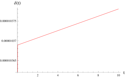
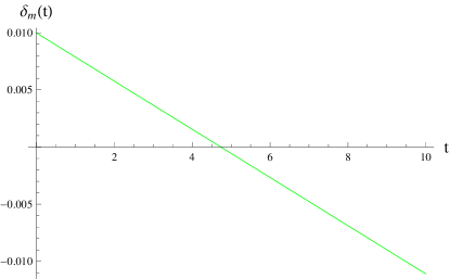
Figure 1: Evolution of perturbations $\delta(t)$ and $\delta_{m}(t)$ for model (17) with $\omega=0$.

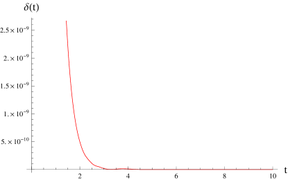
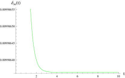
Figure 2: Evolution of perturbations $\delta(t)$ and $\delta_{m}(t)$ for model (18) with $\omega=0$.

Figure 1 shows smooth behavior of $\delta(t)$ (left) and $\delta_{m}(t)$ (right) which do not decay in late times indicating that de Sitter model (17) is unstable. The stability analysis of model (18) with same integration constants is shown in Figure 2. In the left panel, it is observed that small oscillations are produced about $t=4$ while it decays in late times, thus the model (18) shows stable behavior against perturbations. For model (12), Eq.(40) becomes

$$288H_{0}^{6}F_{\mathcal{GG}}^{0}\ddot{\delta}+864H_{0}^{7}F_{\mathcal{GG}}^{0}\dot{\delta}+\left(-6H_{0}^{2}-1152H_{0}^{8}F_{\mathcal{GG}}^{0}\right)\delta$$ (41)

$$+ \left(\kappa^{2}\rho_{*}+\frac{1}{2}\rho_{*}(3-\omega)\mathcal{F}_{T}^{0}+\rho_{*}^{2}(1-3\omega)(1+\omega)\mathcal{F}_{TT}^{0}\right)\delta_{m}=0.$$

Figure 3 represents the behavior of $\delta(t)$ and $\delta_{m}(t)$ for model (21) with integration constants $\hat{c}_{1}=-10,~{}\hat{c}_{2}=0.001$ and $\hat{c}_{3}=1$. It is shown that oscillations in perturbation parameters are produced initially as shown in Figure 3. This oscillating behavior is clearly observed in Figure 4 which decays in future for both $\delta(t)$ as well as $\delta_{m}(t)$ and hence the solution becomes stable.

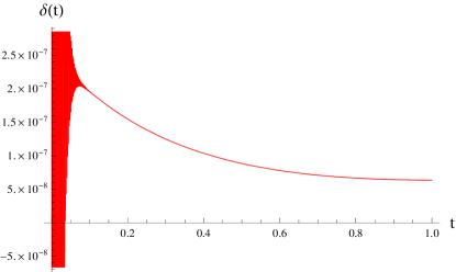
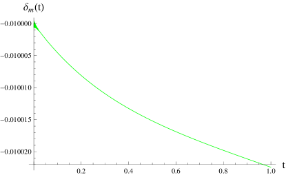
Figure 3: Evolution of perturbations $\delta(t)$ and $\delta_{m}(t)$ for model (21) with $\omega=0$.

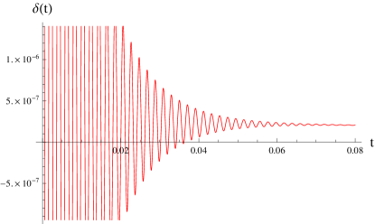
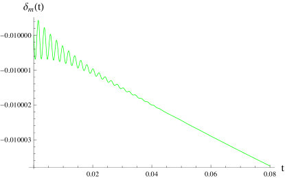
Figure 4: Evolution of perturbations $\delta(t)$ and $\delta_{m}(t)$ for model (21) with $\omega=0$.

4.2 Stability of Power-law Solutions

Here we investigate the stability of power-law solutions. These solutions describe the accelerated as well as decelerated cosmological evolutionary phases in the background of FRW universe. We first consider the reconstructed power-law solution (26) and numerically solve Eqs.(37) and (39). For this model, we choose integration constants $\tilde{c}_{1}=10,~{}\tilde{c}_{2}=-0.5$ and $\tilde{c}_{3}=-1000.$ Figure 5 shows the oscillating behavior of perturbed parameters $(\delta(t),~{}\delta_{m}(t))$ for the cosmic accelerated era with $\omega=-0.5$ and $\lambda=2$. The perturbations around the power-law solutions decay in future leading to stable results. The radiation ($\lambda=1/2$ and $\omega=1/3$) as well as matter ($\lambda=2/3$ and $\omega=0$) dominated eras cannot be discussed for the model (26) because singular as well as complex terms appear which lead to non-physical case.

Secondly, we consider the model (27) and analyze its behavior against linear perturbations. Figure 6 shows the fluctuating behavior of considered perturbations in the cosmic accelerated phase with $\omega=-0.5$ and $\lambda=2$. Here, we choose $\tilde{c}_{1}=0.001,~{}\tilde{c}_{2}=-0.61$ and $\tilde{c}_{3}=-1000.$ It is observed that the oscillating behavior disappears in future while both perturbation parameters will not decay in late times leading to unstable cosmological solutions. The considered model cannot explain the cosmological evolution corresponding to matter and radiation dominated eras like previous model (26).

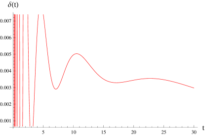
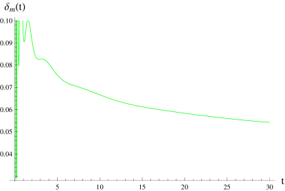
Figure 5: Evolution of perturbations $\delta(t)$ and $\delta_{m}(t)$ for model (26) with $\omega=-0.5$ and $\lambda=2$.

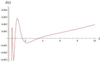
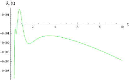
Figure 6: Evolution of perturbations $\delta(t)$ and $\delta_{m}(t)$ for model (27) with $\omega=-0.5$ and $\lambda=2$.

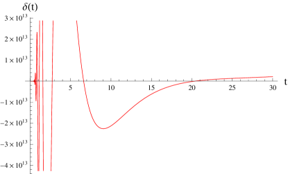
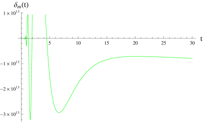
Figure 7: Evolution of perturbations $\delta(t)$ and $\delta_{m}(t)$ for model (28) with $\omega=-0.5$ and $\lambda=1.1$.

Lastly, we explore the stability of model (28) with integration constants $\bar{c}_{1}=-2,~{}\bar{c}_{2}=-0.6,~{}\bar{c}_{3}=1000$ and $\bar{c}_{4}=0.01$. Figure 7 represents the evolution of ($\delta,~{}\delta_{m}$) versus time for $\lambda=1.1$ with $\omega=-0.5$. The left panel shows that the oscillations of $\delta(t)$ decay in late times while fluctuations of $\delta_{m}(t)$ remain present in future. Since a complete perturbation against any cosmological solution includes the matter perturbations therefore, the solutions are unstable.

5 Concluding Remarks

In this paper, we have employed the reconstruction scheme to $f(\mathcal{G},T)$ gravity in the background of isotropic and homogeneous universe model to reproduce some important cosmological models. The basic aspect of this modified gravity is the coupling between curvature and matter components which yields non-zero divergence of the energy-momentum tensor. We have imposed additional constraint to obtain the standard conservation equation which has been used to explain the cosmic evolution in this gravity.

The de Sitter and power-law solutions have been reconstructed for general as well as particular cases which are of great interest and have significant importance in cosmology. We have also reconstructed the $f(\mathcal{G},T)$ model which can explain cosmic history of the phantom as well as non-phantom phases of the universe. Similar reconstruction technique is carried out for $\Lambda$CDM model and found that this gravity fails to reproduce it for both general as well as particular $f(\mathcal{G},T)$ forms. The results are summarized in Table 1. In this table, $\checkmark$ and $\times$ represent that $f(\mathcal{G},T)$ gravity reproduces and fails to reproduce the corresponding cosmological backgrounds, respectively.

Table 1: Cosmological evolution in $f(\mathcal{G},T)$ gravity.

Cosmological Backgrounds	General $f(\mathcal{G},T)$ Model	Particular $f(\mathcal{G},T)$ Model
de Sitter Universe	$\checkmark$	$\checkmark$
Power-law Solutions	$\checkmark$	$\checkmark$
Phantom/non-Phantom Eras	$\times$	$\checkmark$

On physical grounds, the stability analysis of different forms of generic function leads to classify the modified theories of gravity. We have applied the first order perturbations to Hubble parameter and energy density to analyze the stability of models which reproduce de Sitter and power-law cosmic history. We have perturbed the field equation as well as conservation law whose numerical solutions provide the stable/unstable results.

• For the de Sitter universe, the evolution of perturbation has been plotted against time as shown in Figures 1-4. These indicate that models (18) and (21) are stable against linear perturbations.

• For the power-law universe, the stability analysis is given in Figures 5-7. It is found that $f(\mathcal{G},T)$ gravity fails to reproduce matter and radiation dominated eras while stable results are obtained for accelerated phase of the universe for model (26).

We conclude that the cosmological reconstruction and stability analysis might restrict $f(\mathcal{G},T)$ gravity in the background of FRW universe. It would be interesting to discuss ghost instabilities due to the presence of curvature-matter coupling.

Appendix A

The expressions for $\Xi_{i}$’s in Eqs.(17) and (18) are

$$\Xi_{1} = 18c_{1}H_{0}^{4}[8c_{1}H_{0}^{4}\{2(2+59\omega^{2})-11\omega(5-3\omega^{2})\}-(1-11\omega)(1-\omega^{2})]$$

$$\times [1+\omega-36c_{1}H_{0}^{4}(1-3\omega)]^{-2},$$

$$\Xi_{2} = 18c_{1}H_{0}^{4}[(1-11\omega)(1-\omega^{2})-8c_{1}H_{0}^{4}\{2(2+59\omega^{2})-11\omega(5-3\omega^{2})\}]$$

$$\times [(1+\omega)(1-24c_{1}H_{0}^{4})\{1+\omega-6c_{1}H_{0}^{4}(5-4\omega-33\omega^{2})\}]^{-1},$$

$$\Xi_{3} = -[18c_{1}H_{0}^{4}(1-32c_{1}H_{0}^{4})-3\omega\{1-6c_{1}H_{0}^{4}(3-352c_{1}H_{0}^{4})\}$$

$$- 2\omega^{2}\{1-9c_{1}H_{0}^{4}(7-1248c_{1}H_{0}^{4})\}+\omega^{3}\{1-54c_{1}H_{0}^{4}(7-480c_{1}H_{0}^{4})\}]$$

$$\times [(1-3\omega)(1-24c_{1}H_{0}^{4})\{1+\omega-6c_{1}H_{0}^{4}(5-4\omega-33\omega^{2})\}]^{-1}.$$

The values for $\gamma_{\hat{j}}$’s in Eq.(25) are

$$\gamma_{1} = \frac{1}{2}\left[5-\lambda\{1+3\tilde{c}_{2}(1+\omega)\}\right],$$

$$\gamma_{2} = \left[\frac{3}{4}\lambda\tilde{c}_{2}(1+\omega)\{3\tilde{c}_{2}\lambda(1+\omega)+2(\lambda-1)-8\}+\frac{1}{4}(\lambda-1)(\lambda+7)+4\right.$$

$$+ \left.8\tilde{c}_{2}(\lambda-1)\left(\frac{1+\omega}{1-3\omega}\right)\right]^{\frac{1}{2}},\quad\gamma_{3}=-\frac{1}{2}\left(\frac{1-3\omega}{1+\omega}\right),\quad\gamma_{4}=\frac{2\kappa^{2}}{\omega-3},$$

$$\gamma_{5} = \left(\frac{18\lambda^{3}(1-3\omega)^{\frac{3\lambda(1+\omega)-2}{3\lambda(1+\omega)}}}{3\lambda(1-3\omega)+4}\right)\rho_{0}^{\frac{-2}{3\lambda(1+\omega)}},\quad\gamma_{6}=\frac{2}{3\lambda(1+\omega)}.$$

The expressions for $\Delta_{k}$’s and $\Omega_{k}$’s in Eqs.(26) and (27) are

$$\Delta_{1} = 1-\frac{\gamma_{7}}{\gamma_{8}},\quad\Delta_{2}=1-\frac{\gamma_{3}^{2}}{\gamma_{8}},\quad\Delta_{3}=\gamma_{4}\left(1-\frac{1}{\gamma_{8}}\right),\quad\Delta_{4}=\gamma_{5}\left(1-\frac{\gamma_{6}^{2}}{\gamma_{8}}\right),$$

$$\Omega_{1} = 1-\frac{\gamma_{8}}{\gamma_{7}},\quad\Omega_{2}=1-\frac{\gamma_{3}^{2}}{\gamma_{7}},\quad\Omega_{3}=\gamma_{4}\left(1-\frac{1}{\gamma_{7}}\right),\quad\Omega_{4}=\gamma_{5}\left(1-\frac{\gamma_{6}^{2}}{\gamma_{7}}\right),$$

where

$$\gamma_{7} = \frac{\tilde{c}_{2}}{6\lambda}\left[6\tilde{c}_{2}\lambda(1+\omega)^{2}-3\lambda(1+5\omega+2\omega^{2})+2(\gamma_{1}+\gamma_{2})\right],$$

$$\gamma_{8} = \frac{\tilde{c}_{2}}{6\lambda}\left[6\tilde{c}_{2}\lambda(1+\omega)^{2}-3\lambda(1+5\omega+2\omega^{2})+2(\gamma_{1}-\gamma_{2})\right].$$

The values of $\chi_{h}$’s in Eq.(37) are given as follows

$$\chi_{1} = 288H_{*}^{6}f_{\mathcal{GG}}^{*},$$

$$\chi_{2} = 288H_{*}^{5}(3H_{*}^{2}+5\dot{H}_{*})f_{\mathcal{GG}}^{*}+6912H_{*}^{7}(4H_{*}^{2}\dot{H}_{*}+2\dot{H}_{*}^{2}+H_{*}\ddot{H}_{*})f_{\mathcal{GGG}}^{*}$$

$$+ 24(1+\omega)\rho_{*}H_{*}^{3}f_{\mathcal{G}T}^{*}-864(1+\omega)(1-3\omega)H_{*}^{7}\rho_{*}f_{\mathcal{GG}T}^{*},$$

$$\chi_{3} = -6H_{*}^{2}-24H_{*}^{2}\dot{H}_{*}f_{\mathcal{G}}^{*}-288H_{*}^{4}(4H_{*}^{4}-23H_{*}^{2}\dot{H}_{*}-11\dot{H}_{*}^{2}-6H_{*}\ddot{H}_{*})f_{\mathcal{GG}}^{*}$$

$$+ 6912H_{*}^{6}(4H_{*}^{2}+\dot{H}_{*})(4H_{*}^{2}\dot{H}_{*}+2\dot{H}_{*}^{2}+H_{*}\ddot{H}_{*})f_{\mathcal{GGG}}^{*}+12(1+\omega)\rho_{*}H_{*}^{2}$$

$$\times [2(4H_{*}^{2}+\dot{H}_{*})-9(1-3\omega)H_{*}^{2}]f_{\mathcal{G}T}^{*}-864(1+\omega)(1-3\omega)\rho_{*}H_{*}^{6}(4H_{*}^{2}$$

$$+ \dot{H}_{*})f_{\mathcal{GG}T}^{*},$$

$$\chi_{4} = 12(1-3\omega)\rho_{*}H_{*}^{3}f_{\mathcal{G}T}^{*},$$

$$\chi_{5} = \kappa^{2}\rho_{*}-\frac{1}{2}(\omega-3)\rho_{*}f_{T}^{*}+(1-3\omega)(1+\omega)\rho_{*}^{2}f_{TT}^{*}-12(1-3\omega)\rho_{*}H_{*}^{2}$$

$$\times [(4+3\omega)H_{*}^{2}+\dot{H}_{*}]f_{\mathcal{G}T}^{*}+288(1-3\omega)\rho_{*}H_{*}^{4}(4H_{*}^{2}\dot{H}_{*}+2\dot{H}_{*}^{2}+H_{*}\ddot{H}_{*})$$

$$\times f_{\mathcal{GG}T}^{*}-36(1+\omega)(1-3\omega)^{2}\rho_{*}^{2}H_{*}^{4}f_{\mathcal{G}TT}^{*}.$$

The expressions for $\Upsilon_{h}$’s are

$$\Upsilon_{1} = 3(1+\omega)\rho_{*}H_{*}(\kappa^{2}+f_{T})-12(1+\omega)\rho_{*}H_{*}\left[3H_{*}^{2}(1-\omega)(4H_{*}^{2}+\dot{H}_{*})\right.$$

$$- \left.2(16H_{*}^{2}\dot{H}_{*}+6\dot{H}_{*}^{2}+3H_{*}\ddot{H}_{*})\right]f_{\mathcal{G}T}^{*}-72\rho_{*}^{2}H_{*}^{2}(1-3\omega)(1+\omega)^{2}(4H_{*}^{2}$$

$$+ \dot{H}_{*})f_{\mathcal{G}TT}^{*}+576\rho_{*}H_{*}^{3}(1+\omega)(4H_{*}^{2}+\dot{H}_{*})(4H_{*}^{2}\dot{H}_{*}+2\dot{H}_{*}^{2}$$

$$+ 4H_{*}\ddot{H}_{*})f_{\mathcal{GG}T}^{*},$$

$$\Upsilon_{2} = -12\rho_{*}H_{*}^{2}(1+\omega)\left[3H_{*}^{2}(1-\omega)-4(2H_{*}^{2}+3\dot{H}_{*})\right]f_{\mathcal{G}T}^{*}+576\rho_{*}H_{*}^{2}$$

$$\times (1+\omega)(4H_{*}^{2}\dot{H}_{*}+2\dot{H}_{*}^{2}+H_{*}\dot{H}_{*})f_{\mathcal{GG}T}^{*}-72\rho_{*}^{2}H_{*}^{4}(1-3\omega)$$

$$\times (1+\omega^{2})f_{\mathcal{G}TT}^{*},$$

$$\Upsilon_{3} = 24\rho_{*}H_{*}^{3}(1+\omega)f_{\mathcal{G}T}^{*},$$

$$\Upsilon_{4} = -\frac{3}{2}\rho_{*}H_{*}(1+\omega)\left[(1-\omega)f_{T}^{*}+2\rho_{*}^{2}(1+\omega)(1-3\omega)^{2}f_{TTT}^{*}\right]-\frac{15}{2}\rho_{*}^{2}H_{*}$$

$$\times (1-3\omega)(1+\omega)^{2}f_{TT}^{*}+24\rho_{*}H_{*}(1+\omega)(4H_{*}^{2}\dot{H}_{*}+2\dot{H}_{*}^{2}+H_{*}\ddot{H}_{*})$$

$$\times \left[f_{\mathcal{G}T}^{*}+\rho_{*}(1-3\omega)f_{TT\mathcal{G}}^{*}\right],$$

$$\Upsilon_{5} = \rho_{*}\left(\kappa^{2}+\frac{1}{2}(3-\omega)f_{T}^{*}\right)+(1+\omega)(1-3\omega)\rho_{*}^{2}f_{TT}^{*}.$$

For model (12), the coefficients of $(\delta,~{}\delta_{m})$ have the following expressions

$$\hat{\chi}_{1} = 288H_{*}^{6}F_{\mathcal{GG}}^{*},$$

$$\hat{\chi}_{2} = 288H_{*}^{5}(3H_{*}^{2}+5\dot{H}_{*})F_{\mathcal{GG}}^{*}+6912H_{*}^{7}(4H_{*}^{2}\dot{H}_{*}+2\dot{H}_{*}^{2}+H_{*}\ddot{H}_{*})F_{\mathcal{GGG}}^{*},$$

$$\hat{\chi}_{3} = -6H_{*}^{2}-24H_{*}^{2}\dot{H}_{*}F_{\mathcal{G}}^{*}-288H_{*}^{4}(4H_{*}^{4}-23H_{*}^{2}\dot{H}_{*}-11\dot{H}_{*}^{2}-6H_{*}\ddot{H}_{*})$$

$$\times F_{\mathcal{GG}}^{*}+6912H_{*}^{6}(4H_{*}^{2}+\dot{H}_{*})(4H_{*}^{2}\dot{H}_{*}+2\dot{H}_{*}^{2}+H_{*}\ddot{H}_{*})F_{\mathcal{GGG}}^{*},$$

$$\hat{\chi}_{5} = \kappa^{2}\rho_{*}-\frac{1}{2}(\omega-3)\rho_{*}\mathcal{F}_{T}^{*}+(1-3\omega)(1+\omega)\rho_{*}^{2}\mathcal{F}_{TT}^{*},$$

$$\hat{\Upsilon}_{1} = 3(1+\omega)\rho_{*}H_{*}(\kappa^{2}+\mathcal{F}_{T}),$$

$$\hat{\Upsilon}_{4} = -\frac{3}{2}\rho_{*}H_{*}(1+\omega)\left[(1-\omega)\mathcal{F}_{T}^{*}+2\rho_{*}^{2}(1+\omega)(1-3\omega)^{2}\mathcal{F}_{TTT}^{*}\right]-\frac{15}{2}\rho_{*}^{2}H_{*}$$

$$\times (1-3\omega)(1+\omega)^{2}\mathcal{F}_{TT}^{*},$$

$$\hat{\Upsilon}_{5} = \rho_{*}\left(\kappa^{2}+\frac{1}{2}(3-\omega)\mathcal{F}_{T}^{*}\right)+(1+\omega)(1-3\omega)\rho_{*}^{2}\mathcal{F}_{TT}^{*}.$$

References

- [1] Deruelle, N.: Nucl. Phys. B 327(1989)253; Deruelle, N. and Faria-Busto, L.: Phys. Rev. D 41(1990)3696.
- [2] Bhawal, B. and Kar, S.: Phys. Rev. D 46(1992)2464; Deruelle, N. and Doleel, T.: Phys. Rev. D 62(2000)103502.
- [3] De Felice, A. and Tsujikawa, S.: Living Rev. Rel. 13(2010)3.
- [4] Antoniadis, I., Rizos J. and Tamvakis, K.: Nucl. Phys. B 415(1994)497; Nojiri, S., Odintsov, S.D. and Sasaki, M.: Phys. Rev. D 71(2005)123509.
- [5] Nojiri, S. and Odintsov, S.D.: Phys. Lett. B 631(2005)1.
- [6] Cognola, G. et al.: Phys. Rev. D 73(2006)084007; De Felice, A. and Tsujikawa, S.: Phys. Lett. B 675(2009)1; Phys. Rev. D 80(2009)063516.
- [7] Harko, T. et al.: Phys. Rev. D 84(2011)024020.
- [8] Sharif, M. and Ikram, A.: Eur. Phys. J. C 76(2016)640.
- [9] Shamir, M.F. and Ahmad, M.: Eur. Phys. J. C 77(2017)55.
- [10] Dobado, A. and Maroto, A.L.: Phys. Rev. D 52(1995)1895.
- [11] Nojiri, S. and Odintsov, S.D. and Sáez-Gómez, D.: Phys. Lett. B 681(2009)74.
- [12] Elizalde, E. et al.: Class. Quantum Grav. 27(2010)095007.
- [13] Goheer, N. et al.: Phys. Rev. D 79(2009)121301; Goheer, N., Larena, J. and Dunsby, P.K.S.: Phys. Rev. D 80(2009)061301; Sharif, M. and Zubair, M.: J. Phys. Soc. Jpn. 82(2013)014002.
- [14] Sáez-Gómez, D.: Phys. Rev. D 83(2011)064040.
- [15] Myrzakulov, R., Sáez-Gómez, D. and Tureanu, A.: Gen. Relativ. Gravit. 43(2011)1671.
- [16] Jamil, M. et al.: Eur. Phys. J. C 72(2012)1999.
- [17] de la Cruz-Dombriz, Á. and Sáez-Gómez, D.: Class. Quantum Grav. 29(2012)245014.
- [18] Salako, I.G. et al.: J. Cosmol. Astropart. Phys. 11(2013)060.
- [19] Sharif, M. and Zubair, M.: Gen. Relativ. Gravit. 46(2014)1723.
- [20] Landau, L.D. and Lifshitz, E.M.: The Classical Theory of Fields (Pergamon Press, 1971).
- [21] Houndjo, S.J.M.: Europhys. Lett. 94(2011)49001; Astashenok, A.V. et al.: Phys. Lett.B 709(2012)396.