Cross-correlation of galaxies and galaxy clusters in the Sloan Digital Sky Survey and the importance of non-Poissonian shot noise

Abstract

We present measurements of angular cross power spectra between galaxies and optically-selected galaxy clusters in the final photometric sample of the Sloan Digital Sky Survey (SDSS). We measure the auto- and cross-correlations between galaxy and cluster samples, from which we extract the effective biases and study the shot noise properties. We model the non-Poissonian shot noise by introducing an effective number density of tracers and fit for this quantity. We find that we can only describe the cross-correlation of galaxies and galaxy clusters, as well as the auto-correlation of galaxy clusters, on the relevant scales using a non-Poissonian shot noise contribution.

The values of effective bias we finally measure for a volume-limited sample are $b_{cc}=4.09\pm 0.47$ for the cluster auto-correlation and $b_{gc}=2.15\pm 0.09$ for the galaxy-cluster cross-correlation. We find that these results are consistent with expectations from the auto-correlations of galaxies and clusters and are in good agreement with previous studies. The main result is two-fold: firstly we provide a measurement of the cross-correlation of galaxies and clusters, which can be used for further cosmological analysis, and secondly we describe an effective treatment of the shot noise.

1 Introduction

The cosmological distributions of density and temperature perturbations are well approximated over sufficiently large scales by Gaussian random fields, completely described by their two-point statistics. One of the most powerful tools of modern cosmology is therefore the analysis of two-point correlation functions, which can be measured as auto-correlations on one data set or as cross-correlations between two data sets. The strongest current constraints on the cosmological model are indeed derived from the measurement of the auto-correlation of the temperature anisotropy of the cosmic microwave background. Correlations can also be measured from the distribution of tracers of the matter in the Universe: in the last decades multiple surveys have produced large galaxy catalogues, which allowed high-precision measurements of the galaxy auto-correlation, such as the two degree field (2dF) Galaxy Redshift Survey (Cole et al., 2005; Percival et al., 2001) and the SDSS (York et al., 2000; Tegmark et al., 2004; Hayes et al., 2011; Ho et al., 2012; Beutler et al., 2014; Grieb et al., 2016). Likewise, the availability of large optically-selected galaxy cluster catalogues has led to the measurement of the auto-correlation of galaxy clusters, e.g. from the SDSS catalogue (Huetsi, 2009; Estrada et al., 2009; Miyatake et al., 2016; Baxter et al., 2016; Veropalumbo et al., 2016), and from the REFLEX X-ray survey (Collins et al., 2000; Balaguera-Antolínez et al., 2011). These measurements have also been used to obtain cosmological constraints, for both the REFLEX catalogue (Schuecker et al., 2003) and several cluster samples from the SDSS, such as maxBCG (Mana et al., 2013).

Given the success of auto-correlation measurements and the abundance of different cosmological probes of the density field, it is increasingly interesting to combine probes via cross-correlations. Cross-correlations, such as for example between galaxy surveys and the cosmic microwave background (CMB) temperature and lensing (Giannantonio & Percival, 2014; Giannantonio et al., 2016), or between galaxies and cosmic voids (Hamaus et al., 2014, 2016), provide new information without requiring new observations, and can thus lead to improved and complementary cosmological constraints.

Some measurements of cross-correlation between galaxy clusters and galaxies were attempted in the 1970s and 1980s (Peebles, 1974; Seldner & Peebles, 1977a, b; Lilje & Efstathiou, 1988). These studies were performed on relatively small and non-independent catalogues: the cluster catalogues used by all groups were drawn from Abell (1958) and the galaxy catalogues were either the galaxy counts by Shane & Wirtanen (1967) or by Seldner et al. (1977). The better of these two galaxy catalogues had a resolution of 10 arcmin $\times$ 10 arcmin on about $19\deg^{2}$. These early cross-correlation analyses were therefore limited in their possible applications. Some more recent works measuring galaxy and galaxy-cluster cross-correlations are Croft et al. (1999); Sánchez et al. (2005); Zu & Weinberg (2013).

Hütsi & Lahav (2008) proposed the measurement of the correlation between galaxy clusters and galaxies as an additional cosmological probe, which was later extended by Fedeli et al. (2011). They showed that the cross-correlation of clusters and galaxies could lead to better constraints on cosmological parameters, as well as a better determination of the halo model parameters (Cooray & Sheth, 2002).

In this paper, we measure the cross-correlation between galaxies and clusters derived from the final photometric data release of SDSS (Data Release 8, DR8) (Aihara et al., 2011). When using linear theory and cluster bias, as well as Poissonian shot noise, we find a discrepancy between the theoretical expectations and the measured angular power spectra. We show that this tension can be resolved by adopting a modified treatment of the shot noise.

The outline of this paper is as follows: we describe in Section 2 the theoretical modelling of the angular power spectra, the shot noise, and the cluster bias. In Section 3 we introduce the catalogues and mask used in the analysis, and in Section 4 we present the details of the angular power spectra $C_{l}$ estimation. Section 5 presents the results for the auto- and cross-correlations of galaxies and galaxy clusters. Finally, our summary and outlook are given in Section 6.

2 Theoretical Modelling of the Angular Power Spectra

In order to extract cosmological parameters from the measured galaxy and cluster angular power spectra $C^{\rm data}_{l}$, we need theoretical model predictions $C^{\rm model}_{l}$ that account for systematics and measurement effects affecting the observed correlation functions.

2.1 Angular power spectra of biased tracers

We define the density field of the mass density fluctuations at comoving coordinate $\mathbf{r}$ and at any redshift $z$ as

$$\delta_{m}(\mathbf{r})=\frac{\rho_{m}(\mathbf{r})}{\bar{\rho}_{m}}-1\;,$$ (1)

where $\rho_{m}(\mathbf{r})$ is the spatially varying matter density in the Universe with a mean of ${\bar{\rho}_{m}}$. The matter overdensity $\delta_{m}$ can be related to the galaxy (or cluster) overdensity $\delta_{a}$ (where $a$ denotes a galaxy or cluster sample) via the local bias model (Fry & Gaztanaga, 1993),

$$\delta_{a}(\mathbf{r})\simeq b_{1,a}\delta_{m}(\mathbf{r})+\frac{b_{2,a}}{2}\delta_{m}^{2}(\mathbf{r})+O(\delta_{m}^{3})+\varepsilon_{a}\;,$$ (2)

with linear and non-linear bias parameters $b_{1,a}$, $b_{2,a}$, and a shot noise term $\varepsilon_{a}$.

In Fourier space, we can define the matter, galaxy, or cluster power spectra between any pair of samples $(a,b)$ as:

$$(2\pi)^{3}\delta_{\rm D}(k-k^{\prime})P_{ab}(k)\equiv\langle\delta_{a}(\mathbf{k})\,\delta^{\star}_{b}(\mathbf{k^{\prime}})\rangle\;,$$ (3)

where $\mathbf{k}$ denotes a wave vector of amplitude $k$ and angled brackets indicate an average over all Fourier modes within a given spherical shell and $\delta_{\rm D}$ is the Dirac delta function. Up to linear order and assuming Poissonian shot noise, the galaxy (or cluster) power spectrum can be directly related to the matter power spectrum $P(k)$ ,

$$P_{ab}(k)\simeq b_{1,a}b_{1,b}\,P(k)+\delta^{ab}_{K}\,V/N_{a}$$ (4)

where $\delta_{K}$ is the Kronecker delta, and the shot noise contribution is given by the inverse number density of galaxies (or clusters), $V/N_{a}$.

In this analysis we consider the angular power spectrum $C^{ab}_{l}$, a projection of $P_{ab}(k)$ on the sky. We use the publically available code CLASS (Blas et al., 2011) to generate theoretical predictions for the angular cluster power spectrum. CLASS is a differential equation solver for the hierarchy of Boltzmann equations governing the perturbations in the density of dark matter, baryons, photons and any other relevant particle species. The CLASSgal extension (Di Dio et al., 2013) calculates the angular power spectrum, $C^{ab}_{l}$, for any matter tracer as

$$C^{ab}_{l}=4\pi\int\frac{\rm dk}{k}P_{\rm ini}(k)\Delta_{l}^{a}(k)\Delta_{l}^{b}(k)\>,$$ (5)

where $P_{\mathrm{ini}}$ denotes the (dimensionless) primordial power spectrum and the transfer function for the matter component $\Delta^{a}_{l}(k)$ is given by

$$\Delta^{a}_{l}(k)=\int{\rm d}z\>b_{1,a}\frac{{\rm d}N_{a}}{{\rm d}z}j_{l}(kr(z)){\mathcal{D}}(k,z)\>.$$ (6)

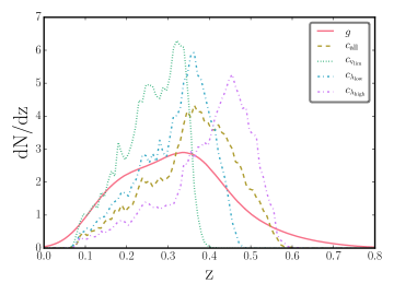
Here $r(z)$ is the comoving distance, ${\mathcal{D}}(k,z)$ the total comoving density fluctuation and we use the galaxy and cluster redshift distributions ${\rm d}N/{\rm d}z$ for the observed sample, which are shown in Figure 2 and introduced in Section 3.

The main goal of this analysis is to measure the auto- and cross-correlation of galaxies and clusters, and to determine the effective bias of these tracers. Therefore we fix the cosmological parameters to their best-fit values as obtained by the Planck collaboration (Planck Collaboration et al., 2014) (Planck2013+WP+highL+BAO), derived by combining their own CMB data with the Wilkinson Microwave Anisotropy Probe (WMAP) polarization data (Bennett et al., 2013), the small-scale CMB measurements from the Atacama Cosmology Telescope (ACT) (Das et al., 2014) and the South Pole Telescope (SPT) (Reichardt et al., 2012), as well as baryonic accoustic oscillations (BAO) data from SDSS (Percival et al., 2010; Padmanabhan et al., 2012; Blake et al., 2011; Anderson et al., 2012; Beutler et al., 2011). The cosmological parameters we use are: $h=0.678$, $\Omega_{\rm b}=0.048$ $\Omega_{\rm c}=0.258$, $\sigma_{8}=0.826$, $z_{\rm re}=11.3$ and $n_{\rm s}=0.96$ (we checked that assuming a Planck 2015 cosmology has no significant impact on the results in our analysis).

For the analysis presented in this paper, we adopt a constant bias model, i.e. we define an effective bias $b_{\rm{eff}}$, such that we can assume for each sample $b_{1,a}(z)=b_{\rm{eff,a}}$. The full redshift evolution of the galaxy and cluster bias could in principle be obtained by subdividing our samples in multiple redshift bins, but this is beyond the scope of the present analysis and the data available.

Note that the CLASS $C^{ab}_{l}$ do not account for a contribution due shot noise. As we demonstrate below, the theoretical power spectra $C^{ab}_{l}$ defined by Equation (5) need a more advanced modelling of the shot noise contribution, which we present in the next Section.

2.2 Accounting for shot noise

Estimating the underlying, continuous dark matter density field via the discrete number density of observed galaxies and clusters, introduces a shot noise contribution which will leave a systematic imprint on the measured angular power spectrum $C^{\rm data}_{l}$. In real space, the Poisson sampling from the true underlying density distribution introduces a contribution to the auto-correlation at zero separation, which translates into the constant contribution in harmonic space shown in Equation (4). Due to the large number of galaxies observed in the SDSS DR8, this contribution to the measured $C_{l}^{\rm data}$ is negligible on the relevant scales for galaxies, but is the leading contribution for the cluster auto-correlation function.

The situation is more complicated for the galaxy-cluster cross-correlation. Galaxies that are part of a cluster contribute to the shot noise, while those that are not part of a cluster do not. Since the majority of the galaxies in our sample are not part of a galaxy cluster, we set the shot noise contribution for the galaxy-cluster cross-correlation to zero for now, but we will revisit this issue in Section 5.2.

Additionally, we have to consider a similar, although smaller, effect for the cross-correlation of clusters in different richness bins. Assuming these clusters occupy halos of different mass, self-pairs are not taken into account in their cross-correlation, resulting in a vanishing Poisson shot noise contribution. We will come back to this issue in Section 5.2 as well.

The Poisson noise contribution to the model power spectra $C_{l}^{ab,\rm model}$ can be approximated by

$${N}_{l}^{ab}=\delta_{K}^{ab}\,f_{\rm sky}\frac{4\pi}{N_{a}}\quad,$$ (7)

where $f_{\rm sky}$ is the fraction of the sky covered and $N_{a}$ is the number of objects observed.

While Equation (7) holds for regular masks, in the case of irregular masks (as the one used in this analysis) a more accurate estimation of the shot noise component is required. In this case, in all generality the shot noise contribution ${\widetilde{N}}_{l}$ can be determined by Poisson sampling different random realisations of a sky map with a constant matter density.

Each random realisation $i$ has a power spectrum $C^{{\rm rand},i}_{l}$, from which an estimate of the shot noise contribution can be obtained by averaging:

$${\widetilde{N}}_{l}=\langle C^{{\rm rand},i}_{l}\rangle\quad,$$ (8)

where the angular bracket $\langle\cdot\rangle$ denotes the average over all random maps $i$. The covariance between different angular wave numbers $l$ and $m$ is given by

$${\rm Cov}[C^{{\rm rand}}_{l},C^{{\rm rand}}_{m}]=\frac{N_{\rm s}}{N_{\rm s}-1}\langle(C^{{\rm rand},i}_{l}-{\widetilde{N}}_{l})(C^{{\rm rand},i}_{m}-{\widetilde{N}}_{m})\rangle$$ (9)

where $N_{\rm s}=100$ is the number of samples used. From this we can determine the covariance of the shot noise, ${\widetilde{N}}$, as

$${\rm Cov}[{\widetilde{N}}_{l},{\widetilde{N}}_{m}]=N^{-1/2}_{s}\,{\rm Cov}[C^{{\rm rand},i}_{l},C^{{\rm rand},i}_{m}]\quad.$$ (10)

We discuss how ${\rm Cov}[{\widetilde{N}}_{l},{\widetilde{N}}_{m}]$ enters the analysis in Section 5.1.

For full sky coverage, we recover the shot noise contribution as given by Equation (7), which remains a good approximation as long as the shape of the mask is regular enough; we expect however to observe signifiant deviations for increasingly irregular masks.

The amplitude of the shot noise contribution ${\widetilde{N}}_{l}$ depends on the number of objects $N_{a}$ distributed over the area of the mask. However, the shape of ${\widetilde{N}}_{l}$ for different $l$ is independent of $N_{a}$, i.e. for a given mask and pixel size, we can determine the shot noise contribution just once then rescale the result according to the actual number of objects observed.

Since we are working with pixellated maps as described in Section 3.2 we will be using the average object per pixel density $\bar{n}$ when determining the shot noise contribution. The shot noise contribution then is determined as

$${\widetilde{N}}_{l}(\bar{n})={\widetilde{N}}_{l}(1)/\bar{n}\quad.$$ (11)

This means that, for a given mask and pixel size, the shot noise contribution can be determined once for a fixed object per pixel density $\bar{n}=1$ and then rescale the result according to the actual object per pixel density of our sample $\bar{n}$. We discuss the actual shot noise contribution for the sky mask used in this analysis in Section 3.2.

2.3 Sub- and super-Poissonian shot noise

We expect deviations from a purely Poissonian shot noise contribution for the power spectra when measured on the galaxy cluster data. $N$-body simulations have provided significant evidence for such deviations in the clustering statistics of dark matter halos (Hamaus et al., 2010). In particular, these deviations have been shown to depend on halo mass: on large scales the shot noise contribution to the power spectrum of low-mass halos exceeds the fiducial value of $V/N_{a}$, while it is suppressed compared to that value at high masses. These effects are commonly referred to as sub- and super-Poissonian shot noise, respectively. In addition, the Poisson expectation is not only found to be violated in auto-correlations of a single tracer, but also in cross-correlations among different tracers. While Poissonian shot noise only affects the auto-correlation of self-pairs, simulations have revealed non-vanishing shot noise contributions in cross-correlations between halos of different mass (Hamaus et al., 2010). These can be either positive or negative, depending on the considered mass ranges.

This phenomenology can be explained with two competing effects: exclusion and non-linear clustering (Baldauf et al., 2013). The former simply specifies the fact that any two tracers, be it halos or galaxies, can never be closer to one another than the sum of their own extents. This violates the Poisson assumption, which states that tracers are randomly sampled at any given point within some volume. Each tracer contributes an exclusion region that effectively diminishes the available sampling volume, and therefore the shot noise contribution. As the exclusion region of halos increases with their mass, high-mass halos are most affected by this. Moreover, the exclusion mechanism also applies for halos of different mass, i.e. it influences cross-correlations of tracers as well.

The first-order contribution from non-linear clustering of halos beyond linear theory is described by the second-order bias parameter $b_{2}$. Besides modifying the scale-dependent linear clustering power spectrum of halos on small scales, it also contributes a scale-independent term that cannot be distinguished from Poisson shot noise (McDonald, 2006). Hence, non-linear clustering effectively increases the Poisson shot noise, and this effect is most important for low-mass halos, where the value of $b_{2}$ is non-zero and exclusion effects are small.

While the above effects mainly apply to dark matter halos, they can be translated to galaxies and clusters by means of the halo model (Seljak, 2000; Smith et al., 2003). Given a Halo Occupation Distribution (HOD), one can assign central and satellite galaxies to each halo of a given mass. While centrals and cluster centers closely obey the effects outlined above, satellites add more complexity as they do not obey halo exclusion. In this case the satellite fraction determines the shot noise as well: a low value ($\sim 5\%$) results in sub-Poissonian, and a high value ($\sim 8.5\%$) in super-Poissonian shot noise (Baldauf et al., 2013).

2.4 Accounting for sub- and super-Poissonian shot noise

We should therefore expect deviations from the Poisson shot noise predictions on all scales, and we expect this correction to be most important for the cluster auto- and cluster-galaxy cross-correlations.

As we have discussed in the previous section, on large scales we expect the shot noise correction to be independent of $l$; we can then model this by introducing an inverse effective (average) number density $\bar{n}_{\rm eff}^{-1}$ free parameter, which we will fit from the data. In this case, we replace $\bar{n}$ in Equation (11) with $\bar{n}_{\rm eff}$ and use the following relation for the effective shot noise:

$${\widetilde{N}}^{\rm eff}_{l}(\bar{n}_{\rm eff})={\widetilde{N}}_{l}(1)\cdot\bar{n}_{\rm eff}^{-1}\quad.$$ (12)

in the case of Poissonian shot noise we should recover $\bar{n}_{\rm eff}\simeq\bar{n}$. We determine $n_{\rm eff}$ for each of the auto- and cross-correlations and marginalise over it to determine the effective bias of each sample.

2.5 Theory predictions for effective bias

We compare the effective bias we extract from the data to theoretical expectations for a volume-limited sample, whose details are described below in Section 5.3. We assume here the halo mass function $n(M,z)$ and halo bias $b(M,z)$ to be given by the fits to $N$-body simulations by Tinker et al. (2008); Tinker et al. (2010). In order to calculate the expected effective bias of a volume-limited cluster sample, we average over the redshift range considered

$$b_{\rm eff} = \left[\int_{\Delta z}\mathrm{d}z\frac{\mathrm{d}V}{\mathrm{d}z\mathrm{d}\Omega}\int\mathrm{d}Mn(M,z)b(M,z)\right.$$

$$\hskip 85.35826pt\left.\int_{\lambda_{\rm min}}\mathrm{d}\lambda P(\lambda|M,z)\right]$$

$$\bigg{/}\left[\int_{\Delta z}\mathrm{d}z\frac{\mathrm{d}V}{\mathrm{d}z\mathrm{d}\Omega}\int\mathrm{d}Mn(M,z)\int_{\lambda_{\rm min}}\mathrm{d}\lambda P(\lambda|M,z)\right]\,,$$

where $\mathrm{d}V/(\mathrm{d}z\mathrm{d}\Omega)$ is the comoving volume element per unit redshift and solid angle, and $P(\lambda|M,z)$ is the probability that a halo of mass $M$ at redshift $z$ is observed with a richness $\lambda$. We model this probability with a log-normal distribution:

$$P(\lambda|M,z)=\frac{1}{\lambda\sqrt{2\pi\sigma_{\ln\lambda}^{2}}}\exp\left[-\frac{\ln\lambda-\langle\ln\lambda(M,z)\rangle}{2\sigma_{\ln\lambda}^{2}}\right]\,,$$ (14)

where we use the parameterisation and parameter values of the scaling relation between mass and richness $\langle\ln\lambda(M,z)\rangle$ as determined by Farahi et al. (2016). The scatter $\sigma_{\ln\lambda}$ is defined as

$$\sigma_{\ln\lambda}^{2}=\frac{\exp\left[\langle\ln\lambda(M,z)\rangle\right]-1}{\left(\exp\left[\langle\ln\lambda(M,z)\rangle\right]\right)^{2}}+\sigma_{\ln\lambda|M}^{2}\,,$$ (15)

where the first term accounts for the richness-dependent Poisson noise and $\sigma_{\ln\lambda|M}$ is the intrinsic scatter in the richness-mass relation. As Farahi et al. (2016) do not specify the value for $\sigma_{\ln\lambda|M}$ or $\sigma_{\ln M|\lambda}$, we determine $\sigma_{\ln\lambda|M}$ using the value for $\sigma_{\ln M|\lambda}=0.25$ from Simet et al. (2016). Using Equations (13) to (15) from Simet et al. (2016), we determine $\sigma_{\ln\lambda|M}$ via the following relation

$$\sigma_{\ln\lambda|M}=\frac{\sigma_{\ln M|\lambda}}{\alpha}\quad,$$ (16)

where $\alpha=1.326$ denotes the power-law slope of mass given the richness, as defined by Simet et al. (2016).

3 Data

3.1 Galaxy and cluster catalogues

We use galaxy and galaxy cluster data drawn from the Sloan Digital Sky Survey (SDSS) (York et al., 2000). The SDSS is conducted with a dedicated 2.5m telescope at the Apache Point Observatory in Southern New Mexico in the United States. This telescope has a wide field of view of $7\deg^{2}$, a large mosaic CCD camera and a pair of double spectrographs (Aihara et al., 2011; Eisenstein et al., 2011). We use the final photometric SDSS data from the eighth data release (DR8) that combines data from the two project phases SDSS-I and SDSS-II.

The full area of SDSS DR8 is $14,555\deg^{2}$ and includes photometric measurements of 208,478,448 galaxies. For the analysis in this paper we use the same galaxy catalogue and selection criteria as in Giannantonio et al. (2012). The catalogue only contains objects with redshift between 0.1 and 0.9 that have a photo-$z$ uncertainty of $\sigma_{z}(z)<0.5\,z$. A completeness cut is applied by only using objects with extinction-corrected $r$-band magnitudes between 18 and 21. After these cuts, the catalogue contains 41,853,880 galaxies.

We use the cluster catalogue constructed from SDSS DR8 with the red-sequence Matched-filter Probabilistic Percolation (redMaPPer) cluster finding algorithm version 5.10 (Rykoff et al., 2014). It contains $\sim 26,350$ galaxy clusters covering a redshift range between 0.1 and 0.6 and contains only clusters with richness $\lambda>20$. Note that we use the richness as defined by redMaPPer throughout this paper. As the richness $\lambda$ is a measure of the number of galaxies within the cluster, this means smaller clusters, which are more strongly affected by systematic errors, are excluded from the analysis.

3.2 Pixellated maps and survey mask

We create pixelized maps for the galaxy and the galaxy cluster catalogues using the pixelization scheme HEALPix (Gorski et al., 2005), in which the resolution is expressed by the parameter $N_{\rm side}$. The pixellation effectively smoothes information on scales smaller than the pixel size, and it can be described by a multiplicative window function $w_{l}$ given by the pixel window function provided by HEALPix.

To construct the (binary) survey mask we follow the method by Giannantonio et al. (2006) to estimate the coverage of pixels that straddle the survey boundaries. If we have a distribution $P(n)$ of the number of galaxies per pixel, this effect causes a deviation from a Poisson distribution $P^{\rm Poiss}(n)$ for low $n$, i.e. we will find an excess of pixels with a small $n$ compared to $P^{\rm Poiss}(n)$. In practice, we create the mask by discarding pixels where $P(n)\not\approx P^{\rm Poiss}(n)$, i.e. pixels with $n<n_{\rm min}$ where $n_{\rm min}$ is a cut-off threshold we choose.

The pixel size we choose is constrained by two factors. On the one hand pixels should be large enough to ensure that the mean of the distribution $P(n)$ is far from zero, i.e. there is only a very small and negligible number of pixels with a small number of galaxies. On the other hand pixels should be small enough so that we can measure the angular power spectra at the scales of interest.

We choose the HEALPix resolution $N_{\rm side}=512$, corresponding to a pixel side of $7^{\prime}$, as this produces an average number of galaxies per pixel of $\bar{n}\simeq 30$ for the SDSS galaxy catalogue, and it also allows access to the scales of interest in this analysis. All catalogues we use here are pixelized at this resolution.

Therefore, to create the mask we first determine the number of galaxies $n_{i}$ in each of the pixels $i$ and discard pixels with zero galaxies. Then we determine the mean and variance of the Poisson distribution by calculating the average number of galaxies per pixel $\bar{n}$ and identify the value of $n$ below which we observe a deviation from the Poisson distribution. We find that $n_{\rm min}=\bar{n}-2\sqrt{\bar{n}}$ (i.e. the equivalent of two standard deviations below the mean number of pixels) is a good value for the cut-off and we mask all pixels where $n_{i}<n_{\rm min}$.

We generate the cluster mask by repeating the above process using the available random redMaPPer cluster catalogues. We choose to only work with the intersection of the galaxy and galaxy cluster masks. We further combine this mask with the dust extinction maps by Schlegel et al. (1998), retaining only pixels with reddening values $E(B-V)<0.2$, and with the SDSS seeing masks by Ross et al. (2011), retaining pixels with seeing values below $1.4^{\prime\prime}$. The final mask footprint covers 6,983 deg². After the application of the complete mask, the data covers a fraction of sky $f_{\rm sky}=0.21$ and contains 671,533 unmasked pixels.

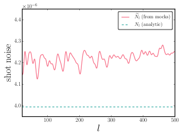
In Section 2.2 we described how we determine the shot noise contribution for a given mask. Figure 1 shows both the analytic shot noise approximation ${N}_{l}$ from Equation (7) and the shot noise ${\widetilde{N}}_{l}$ from Poisson sampling for $\bar{n}=1$ from Equation (8) for the mask used in our analysis. We see that taking into account the effect of the mask increases the shot noise by approximately 5%. Also, there is a mild $l$-dependence of the shot noise for the Poisson sampled shot noise compared to the analytic approximate shot noise caused by the shape of the mask.

Figure 1: Shot noise predictions for an approximate analytic shot noise estimate ${N}_{l}$ (Equation 7) and the Poisson sampled shot noise (mocks) ${\widetilde{N}}_{l}$ (Equation 8) for an average number of objects per pixel density $\bar{n}=1$.

3.3 Subsets of data used

In addition to the full sample described in Section 3.1 above, for our analysis we use different subsets of the cluster catalogue. In the following, we will consider:

• $c_{\rm all}$: the full cluster sample, which is richness-selected and thus not volume-limited;

• $c_{\rm vlim}$: a volume-limited sample that is constructed by using only clusters with $z<0.35$;

• $c_{\lambda_{\rm low}}$ and $c_{\lambda_{\rm high}}$: a low- and high-richness sample, constructed from the full cluster sample (all redshifts) that is split at the median richness of $\lambda_{\rm med}=33.7$.

The different samples are summarised in Table 1. The sample $c_{\rm all}$ containing all the clusters of the redMaPPer catalogue is the starting point of our analysis as it makes use of all the objects available and allows us to investigate the shot noise properties of our measurements, especially for the galaxy and galaxy cluster cross-correlation (Sections 5.1 and 5.2). In a second step we use the $c_{\rm vlim}$ sample in order to be able to compare our best-fit results to the theoretical expectation for the value of the effective bias (Section 5.3). Finally, we use the samples split into two richness bins $c_{\lambda_{\rm low}}$ and $c_{\lambda_{\rm high}}$ to investigate the shot noise properties of cluster clustering (Section 5.4).

Figure 2: Normalized redshift distributions ${\rm d}N/{\rm d}z$ of galaxies and galaxy clusters samples as discussed in Section 3.3.

Table 1: Summary of all samples used in this analysis. $N$ is the total number of objects left after masking and cuts, $\bar{n}$ is the average number of objects per pixel ($N_{\rm side}=512$), $z_{\rm median}$ is the median redshift of the sample and the selection column indicates the additional cuts done beyond masking.

Sample	$N$	object type	$z_{\rm median}$	$\bar{n}$	selection
g	25,959,346	galaxies	0.31	39	see text
$c_{\rm all}$	21,962	clusters	0.37	0.033	none
$c_{\rm vlim}$	9,294	clusters	0.27	0.014	$z<0.35$
$c_{\lambda{\rm low}}$	10,981	clusters	0.34	0.016	$\lambda<33.7$
$c_{\lambda{\rm high}}$	10,981	clusters	0.42	0.016	$\lambda>33.7$

In Figure 2 we show the redshift distribution ${\rm d}N/{\rm d}z$ of galaxies and galaxy clusters, after masking has been applied, for the different samples described above. In order to account for the uncertainties in cluster redshifts when performing the theoretical predictions in Sections 2.1, we randomly sample from the redshifts errors for the respective object type. For galaxies we assume an overall 5% photometric redshift error as the individual redshift errors in the catalogues underestimate the true redshift error. In the case of the galaxy clusters we re-sample the provided redshift according to the error provided by redMaPPer. Therefore the redshift distribution of galaxies does not have a sharp boundary at low redshifts and the distribution of clusters for the $c_{\rm vlim}$ sample does not have a sharp boundary at $z=0.35$.

4 Angular power spectrum estimators

We measure the angular power spectrum $C_{l}$ for all the data products described in Section 3 using the Spatially Inhomogeneous Correlation Estimator for Temperature and Polarisation (PolSpice) (Chon et al., 2004; Szapudi et al., 2000; Challinor & Chon, 2005). The advantage of using PolSpice is that the algorithm corrects for distortions of the measured power spectrum caused by masking and the pixel window function $w_{l}$. The partial sky coverage has more complex effects (see eg Efstathiou, 2004), which we assume here to be corrected by PolSpice.

PolSpice is used to estimate the $C^{\rm data}_{l}$ from pixellated density contrast maps $\delta_{i}$ derived from both the galaxy and galaxy cluster density per pixel $n_{i}$

$$\delta_{i}=\frac{n_{i}}{\bar{n}}-1\,,$$ (17)

where $\bar{n}$ denotes the average over all pixels $i$.

For our analysis we consider multipoles $l$ in the range $20<l<500$. The minimum multipole is limited by the size of the mask and we choose a cautious estimate following La Porta et al. (2008). For the maximum multipole we choose an equally conservative limit by using $l<N_{\rm side}$ instead of $l<2N_{\rm side}$ as reasoned by Gorski et al. (2005).

Following the argument by Pillepich et al. (2012) (and references therein and their Figure 7) we expect the onset of the bias non-linearity at $k>0.2\,h$/Mpc, which corresponds to a multipole $l\approx 200$ at a mean redshift similar to the mean redshift of the cluster samples described in Section 3.3. However, while limiting our analysis to $l<200$ does not change the results significantly, the statistical power of our results is reduced noticeably. Therefore we will use $l<N_{\rm side}$ throughout this paper and perform the cross-check described in Section 5.1 to ensure that the non-linearities do not have a notable effect on our results.

To some extent the non-linearities can be absorbed by the way we treat the shot noise, however this cannot account for the entire mass, scale and redshift dependence of the non-linear bias. Nevertheless, the cross-check discussed in Section 5.1 gives us confidence that any residual non-linearities are sub-dominant, because the scale-dependent bias of tracers with different host halo mass cannot be accounted for in our model and would lead to tensions in the cross-check.

We estimate the covariance of the $C_{l}^{\rm data}$ by using a jack-knife sampling of the maps, which is performed by dividing the map area into $N_{\rm jk}$ regions of equal size. For each sampling $i$ one of the regions is left out and the measurement of the $C^{i}_{l}$ is done on the area constituted by the remaining $N_{\rm jk}-1$ regions. The covariance matrix using jackknife sampling is then given by

$${\rm Cov}^{\rm data}[C_{l},C_{m}]=\frac{N_{\rm jk}-1}{N_{\rm jk}}\sum\limits_{j}{(C^{i}_{l}-\langle C_{l}\rangle)(C^{i}_{m}-\langle C_{m}\rangle)}\,.$$ (18)

The number of jack-knife samples $N_{\rm jk}$ needs to be large enough to determine the covariance matrix with sufficient accuracy for a given number of data bins $N_{\rm bin}$ in $l$-space. Following the reasoning by Taylor et al. (2013), we choose $N_{\rm bin}=$ 20 and $N_{\rm jk}=$ 100 to determine the covariance matrices of the $C_{l}$ measurements. This yields an uncertainty in the error bars of the extracted parameters of 16%.

Note that when calculating the inverse covariance, we need to multiply it by the de-biasing factor introduced by Hartlap et al. (2007) and Taylor et al. (2013):

$$f_{\rm corr}=\frac{N_{\rm jk}-1}{N_{\rm jk}-N_{\rm bin}-2}\quad,$$ (19)

where $N_{\rm bin}$ is the size of the data vector, i.e. the number of $C_{l}$ bins $N_{\rm bin}$. In the following section we will present the results of our analysis.

5 Results

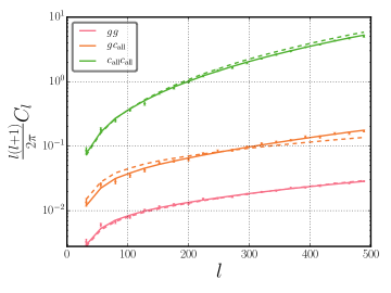
In Figure 3 we present the measured angular power spectra for the galaxy ($gg$), cluster ($c_{\rm all}c_{\rm all}$) and galaxy-cluster ($gc_{\rm all}$) cases using the full cluster sample $c_{\rm all}$ and the analysis method described in Section 4. The best fitting models to these measurements are described in Sections 5.1 and 5.2 below and are shown as lines in Figure 3.

In order to determine the effective bias for the different tracers, we use two different models to account for the shot noise. We first analyse the data using Poissonian shot noise as described in Section 2.2 and discuss the results of those fits. In a second step we account for non-Poissonian shot noise as discussed in 2.4.

5.1 Fitting the angular power spectra with a fixed shot noise contribution

We first fit to the $C^{\rm data}_{l}$ the model given by:

$$C_{l}^{\rm model}(b)=C_{l}^{\rm th}(b)+{\widetilde{N}}_{l}(\bar{n})\quad,$$ (20)

where $C_{l}^{\rm th}$ is the theoretical angular power spectrum as given in Equation (5) for a given value of the effective bias $b$ and ${\widetilde{N}}_{l}(\bar{n})$ is the Poisson noise term given in Equation (7).

For the covariance, there are two contributions: the covariance from the power spectrum measurement given in Equation (18), as well as the covariance from the Poisson noise contribution ${\widetilde{N}}_{l}$ given in Equation (10). The covariance of the shot noise contribution arises from the fact that we determine the shot noise from the PolSpice measurements of random maps as discussed in Section 2.2.

However, ${\rm Cov}[C^{{\rm rand},i}_{l},C^{{\rm rand},i}_{m}]$ is about one order of magnitude smaller than ${\rm Cov}^{\rm data}[C_{l},C_{m}]$ and $N^{-1/2}_{s}=10$, and therefore the covariance originating from the Poisson noise correction ${\rm Cov}[{\widetilde{N}}_{l},{\widetilde{N}}_{m}]$ is about two orders of magnitude smaller than the covariance contribution from the data ${\rm Cov}^{\rm data}[C_{l},C_{m}]$. Hence we neglect the covariance contribution of the shot noise error and use

$${\rm Cov}^{\rm fit}[C_{l},C_{m}]={\rm Cov}^{\rm data}[C_{l},C_{m}]$$ (21)

as the covariance in the Gaussian likelihood ${\mathcal{L}}$ of the effective bias parameters $b$.

We then use this covariance to calculate the Gaussian likelihoods of the effective bias parameters from all spectra we consider, i.e. from galaxy and cluster auto-spectra and from the cross-spectrum; we label these likelihoods ${\mathcal{L}}_{g}$, ${\mathcal{L}}_{gc_{\rm all}}$, and ${\mathcal{L}}_{c_{\rm all}}$ respectively.

Additionally, we can estimate the effective bias likelihood from the cross-correlation given the results from the two corresponding auto-correlations. For example, from the likelihoods of the galaxy and cluster auto-correlations ${\mathcal{L}}_{g}$ and ${\mathcal{L}}_{c}$, we can construct the following likelihood

$${\mathcal{L}}_{\sqrt{b_{g}b_{c}}}(b)=\iint{\rm d}\tilde{b}_{g}{\rm d}\tilde{b}_{c}\,\delta_{\rm D}\left(b-\sqrt{\tilde{b}_{g}\tilde{b}_{c}}\right){\mathcal{L}}_{g}(\tilde{b}_{g}){\mathcal{L}}_{c}(\tilde{b}_{c})\quad.$$ (22)

This likelihood serves as a cross-check for the biases obtained by our analysis and is equivalent to drawing values for $b_{g}$ and $b_{c}$ from the respective auto-correlation distributions and determining a new distribution from the corresponding $\sqrt{b_{g}b_{c}}$. We determine these cross-check likelihoods and bias values for all the cross-correlations we determine in our analysis.

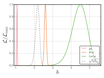
We start by analysing the auto- and cross-correlations for the largest samples available, i.e. the galaxy sample $g$ and the full cluster sample $c_{\rm all}$, as we expect to obtain the most accurate measurements from these samples. The best-fit models as defined in Equation (20) are shown as dashed lines in Figure 3. While the galaxy auto-correlation ($gg$) is accurately described by the model, the galaxy-cluster cross-correlation ($gc_{\rm all}$) as well as the cluster auto-correlation ($cc_{\rm all}$) are poorly described by the fit. Best-fit parameters, as well as $\chi^{2}$, are listed in rows 1 – 3 of Table 2. Note that the $\chi^{2}$ values are too large for the $gc_{\rm all}$ and $c_{\rm all}c_{\rm all}$ correlations, indicating that the model is not a good description of the measurements. The likelihoods for the fits and cross-check are shown in Figure 4 and indicate that also ${\mathcal{L}}_{\sqrt{b_{g}b_{c}}}$ does not agree well with the results for ${\mathcal{L}}_{g}$ and ${\mathcal{L}}_{c}$, i.e. the results of the auto- and cross-correlations are inconsistent with each other.

Table 2: Results for the different parameter fits from the angular power spectra we use. Column 2 indicates the correlator used, column 3 indicates the maximum likelihood value for bias $b$ and the statistical error for the fit, column 4 the $\chi^{2}$ and number of degrees of freedom. If the effective noise contribution is also determined in the fit, the inverse of the maximum likelihood effective pixel density $\bar{n}^{\rm eff,ML}$ is listed in column 5, while column 6 lists the actual inverse pixel density of objects $\bar{n}^{-1}$ (only available for auto-correlations). In case the cross-check can be performed, the corresponding value for bias $b_{\rm cross-check}$ (including error) is listed in column 7.

Row	correlator	$b$ $\pm$ $\sigma_{\rm stat}$	$\chi^{2}$/dof	$1/\bar{n}^{\rm eff}\pm\sigma_{\rm stat}$	$1/\bar{n}$	$b_{\rm cross-check}$
1	$gg$	1.07 $\pm$ 0.02	24.1/19	–	0.026	–
2	$gc_{\rm all}$	2.60 $\pm$ 0.05	216/19	–	–	2.19 $\pm$ 0.10
3	$c_{\rm all}c_{\rm all}$	4.50 $\pm$ 0.42	48.9/19	–	30.3	–
4	$gg$	1.10 $\pm$ 0.03	11.8/18	0.013 $\pm$ 0.011	0.026	–
5	$gc_{\rm all}$	2.29 $\pm$ 0.09	18.3/18	0.405 $\pm$ 0.086	–	2.30 $\pm$ 0.10
6	$c_{\rm all}c_{\rm all}$	4.82 $\pm$ 0.41	14.0/18	27.0 $\pm$ 1.90	30.3	–
7	$gc_{\rm vlim}$	2.15 $\pm$ 0.09	22.0/18	0.610 $\pm$ 0.111	–	2.12 $\pm$ 0.13
8	$c_{\rm vlim}c_{\rm vlim}$	4.09 $\pm$ 0.47	8.0/18	66.3 $\pm$ 0.067	71.4	–
9	$gc_{\lambda_{\text{low}}}$	2.11 $\pm$ 0.10	17.8/18	0.314 $\pm$ 0.107	–	2.09 $\pm$ 0.13
10	$gc_{\lambda_{\text{high}}}$	2.53 $\pm$ 0.13	9.43/18	0.516 $\pm$ 0.119	–	2.50 $\pm$ 0.15
11	$c_{\lambda_{\text{low}}}c_{\lambda_{\text{low}}}$	3.99 $\pm$ 0.48	13.3/18	57.0 $\pm$ 3.64	62.5	–
12	$c_{\lambda_{\text{high}}}c_{\lambda_{\text{high}}}$	5.72 $\pm$ 0.65	9.48/18	57.6 $\pm$ 4.14	62.5	–
13	$c_{\lambda_{\text{low}}}c_{\lambda_{\text{high}}}$	4.98 $\pm$ 0.57	11.0/18	-3.69 $\pm$ 1.60	–	4.71 $\pm$ 0.41

Figure 3: Galaxy ($gg$ – red lines and symbols), cluster ($c_{\rm all}c_{\rm all}$ – green lines and symbols) and galaxy-cluster ($gc_{\rm all}$ – orange lines and symbols) angular power spectra for the data described in Section 3. Lines indicate the best-fit models described in Sections 5.1 and 5.2: dashed lines show the best-fit model specified in Equation (20) using Poissonian shot noise, while solid lines use the best-fit model specified in Equation (23) where $\bar{n}^{\rm eff}$ is added as a fit parameter to adjust the shot noise contribution.

Figure 4: Likelihood functions for the effective bias of the samples we consider, obtained using a fixed shot noise contribution, for galaxies ($gg$ – red lines), clusters ($c_{\rm all}c_{\rm all}$ – green lines) and galaxy-clusters ($gc_{\rm all}$ – brown lines), as well as for the cross-check case ${\mathcal{L}}_{\sqrt{b_{g}b_{c}}}$ ($\sqrt{b_{g}b_{c}}$ - dashed grey line) described in Section 5.1.

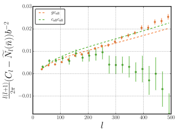
Concentrating on the mismatch between the data and model for the galaxy-cluster ($gc_{\rm all}$) and cluster ($c_{\rm all}c_{\rm all}$) correlation, we remove the shot noise contribution, which is dominant for the $c_{\rm all}c_{\rm all}$ correlation, from both the data and model. In addition, we bring the $C_{l}$ to the same scale by renormalizing them by the best fit bias; the resulting $C_{l}$ are shown in Figure 5.

For the galaxy-cluster cross-correlation, the model (orange symbols and line) clearly overestimates the $C_{l}$ for low $l$ and underestimates them for high $l$. This is not unexpected, because neglecting the shot noise contribution for the galaxies that are part of clusters (as discussed in Section 2.2) is expected to be a poor approximation.

In the case of the cluster auto-correlation, we can now see the mismatch between the data and model more clearly because the extracted signal is dominated by the shot noise. Also in this case, the figure shows a severe mismatch, as the model overestimates the $C_{l}$ on all scales. Above $l\approx 400$ the noise-corrected $C_{l}$ even turn negative, indicating the shot noise is overcorrected using the average object per pixel density $\bar{n}$ for clusters.

Figure 5: Cluster ($c_{\rm all}c_{\rm all}$) and galaxy-cluster ($gc_{\rm all}$) power spectra with Poissonian shot noise ${\widetilde{N}}_{l}$ removed according to Equation (11) and rescaled by the best-fit bias $b$. Dashed lines show the best-fit model specified in Equation (20).

5.2 Accounting for the effective noise contribution

Following the reasoning of Section 2.4, we can effectively account for a modification of the shot noise contribution if we limit ourselves to a regime where the correction is (to a good approximation) independent of $l$. We can then introduce an effective number density of objects per pixel $\bar{n}^{\rm eff}$ as a nuisance parameter. This allows us to account for any sub- and super-Poissonian shot noise contributions where the shape of the shot noise correction is unaffected and only the magnitude of $\widetilde{N}_{l}$ is adjusted, i.e.

$$C_{l}^{\rm model}(b,\bar{n}^{\rm eff})=C_{l}^{\rm th}(b)+{\widetilde{N}}_{l}(\bar{n}^{\rm eff})\quad.$$ (23)

To account for measuring systematics affecting the power spectra, a similar treatment was used by Ho et al. (2012); Zhao et al. (2013); Beutler et al. (2014); Johnson et al. (2016); Grieb et al. (2016) in their analyses.

The results for the fits including the effective shot noise contribution as a free parameter are shown as the solid lines in Figure 3. The $C^{\rm model}_{l}(b,\bar{n}^{\rm eff})$ for the fit describe the data much more accurately. The corresponding constant likelihood contours are shown in Figure 6 where the dashed lines indicate the actual $1/\bar{n}$ for the Poissonian shot noise contribution (not applicable to the cross-correlation $gc_{\rm all}$). Both the galaxy and cluster auto-correlations slightly favour sub-Poissonian noise contributions, though the deviation from the Poissonian noise case is below 1-$\sigma$ for galaxies and about 1.5-$\sigma$ for the clusters. As expected, the noise contribution for the galaxy auto-correlation is small. However, the shot noise for the cluster auto-correlation is a dominant contribution, and therefore we see a much better description of the data compared to the previous fit where we only fitted for the bias. The same holds for the galaxy-cluster cross-correlation for which the data clearly favours a non-zero shot noise contribution.

Figure 6: The 2d-likelihoods for the fits described in Section 5.2 for the parameters bias $b$ and effective number of objects per pixel $\bar{n}^{\rm eff}$. Solid lines indicate the $68\%$, $95\%$ and $99\%$ confidence regions respectively. For the auto-correlation cases the dotted lines indicate the actual inverse number of objects per pixel $\bar{n}^{-1}$.

Figure 7: Likelihoods of the effective bias, marginalised over the amplitude of the shot noise contribution as described in Section 5.2, for the different correlators we consider: galaxies auto- ($gg$ – red lines), clusters auto- ($c_{\rm all}c_{\rm all}$ – green lines) and galaxy-cluster cross-correlation ($gc_{\rm all}$ – brown lines) as well as the consistency check bias ($\sqrt{b_{g}b_{c}}$ – dashed grey line) as described in Section 5.1.

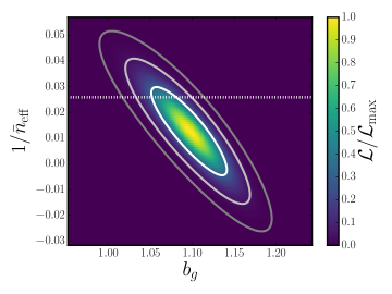
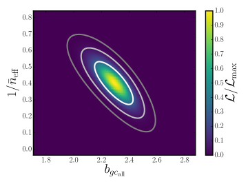
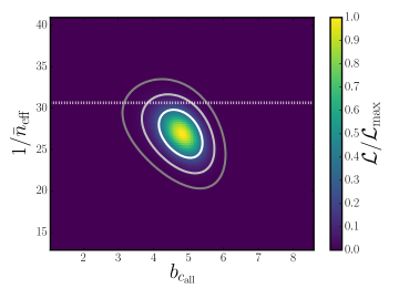
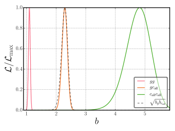
We show in Figure 7 the marginalised likelihoods for the bias parameters; we can see that in this case the cross-check likelihood ${\mathcal{L}}_{\sqrt{b_{g}b_{c}}}$ agrees well with the result obtained from the galaxy-cluster cross-correlation $gc_{\rm all}$. This means that the measurements of auto- and cross-correlation are now in good agreement with each other when introducing $n_{\rm eff}$ as an additional model parameter.

The results of these fits, including maximum likelihood values for ${\mathcal{L}}_{\sqrt{b_{g}b_{c}}}$, are summarised in rows 4-6 of Table 2. Note that the $\chi^{2}$ have improved significantly compared to the bias-only fits.

The fact that we obtain a sub-Poissonian shot noise from the auto-correlation of galaxies argues for a relatively low satellite fraction in the sample, as discussed in Section 2.3. The sub-Poissonian shot noise obtained from the cluster auto-correlation is expected because clusters obey halo exclusion.

5.3 Effective bias for volume-limited cluster sample

The measurement of the cluster auto-correlation for the full sample $c_{\rm all}$ yields a bias value of $b_{c}=4.82\pm 0.41$. However, the $c_{\rm all}$ sample is not volume-limited and we should therefore use the volume-limited sample $c_{\rm vlim}$ when comparing the effective bias to theoretical expectations.

We perform the same analysis of Section 5.2 on the volume-limited sample $c_{\rm vlim}$ as discussed in Section 3 and summarized in Table 1. The fits for the volume-limited cluster sample are qualitatively similar to the $c_{\rm all}$ samples and we therefore do not show plots of the power spectra and best fits. Results for the auto-correlation $c_{\rm vlim}c_{\rm vlim}$ as well as the cross-correlation $gc_{\rm vlim}$ are listed in rows 7 and 8 of Table 2. The bias from the cross-check and the bias for the cross-correlation are again in agreement. From the cluster auto-correlation we find $b_{c_{\rm vlim}}=4.09\pm 0.47$.

From the theoretical modeling of the effective bias in Section 2.5 we expect $b\approx 2.8$ for the volume-limited cluster sample, which is in tension with the value extracted from the data at the 2-3 $\sigma$ level.

5.3.1 Systematics affecting the bias measurement

We explored – and ruled out – the following systematic effects which might explain this discrepancy. The redshift and richness distributions of clusters we expect from the predictions in Section 2.5 are in good agreement with those measured for the volume-limited sample as shown in Figure 2 and cannot be used to explain this discrepancy. Neither are there extremely high mass/bias objects that could explain the difference. We have checked if statistical and systematic uncertainty of the mass-richness relation for galaxy clusters could account for the tension. Even shifting the mass-richness relation by 30% in mass does not alleviate the tension. The effect of the measurement uncertainties of the mass-richness relation parameters is negligible. The measurement error on $\sigma_{8}$ from the Planck2013+WP+highL+BAO measurement also cannot account for the discrepancy, i.e. shifting the value of $\sigma_{8}$ by 1-$\sigma$ does only have a very small effect on our measurement of the effective bias.

In this work we have not explored the effect of assembly bias (Sheth & Tormen, 2004; Gao et al., 2005; Gao & White, 2007; Wechsler et al., 2006; More et al., 2016), i.e. the dependence of halo clustering on assembly history. However, our effective bias measurement is consistent with the results examining this effect as reported in Miyatake et al. (2016) and Baxter et al. (2016) and references therein. Miyatake et al. (2016) split the clusters into two subsamples based on the average member galaxy separation from the cluster center and find significantly different values for the bias for those subsamples: $b=2.17\pm 0.31$ for clusters with a low average member galaxy separation and $b=3.67\pm 0.40$ for large average separation. Baxter et al. (2016) measures the angular correlation function $w(\theta)$ for clusters in different richness and redshift bins and find high (compared to the prediction using the Tinker mass function) bias values between 3 and 5 for the $\lambda>20$ richness bins. It will be very interesting to study this effect in more detail using angular power spectra in harmonic space in a future analysis.

5.4 Results for low and high richness cluster samples

Next, we investigate the shot noise properties in the cross-correlations of clusters in different richness bins and hence different halo mass. Therefore, we divide the $c_{\rm all}$ sample into two halves, splitting it at the median richness $\lambda_{\rm median}=33.7$ with $\lambda_{\rm low}<\lambda_{\rm median}$ and $\lambda_{\rm low}>\lambda_{\rm median}$ with median redshifts 0.315 and 0.42. The redshift distributions for these two sub-samples are shown in Figure 2.

The auto-correlations of the richness-split cluster samples and their relative best-fit bias values are qualitatively similar to the $c_{\rm all}$ sample. We therefore do not show the results for the auto-correlations and will only discuss and show the cross-correlation measurements below. The fit results are summarized in rows 9-13 of Table 2. As expected, for the auto-correlation of the low-richness sample $c_{\lambda_{\rm low}}$ we observe a smaller bias than for the $c_{\rm all}$ sample, while for the high-richness sample $c_{\lambda_{\rm high}}$ the bias is shifted to even higher values (rows 11 and 12). The effective shot noise contribution is larger for these samples as reflected by the smaller values of $\bar{n}_{\rm eff}$, because there are half as many objects in the sub-samples. A similar systematic bias shift can be seen for the galaxy-cluster cross-correlation, which is shown in rows 7-8, while the shot-noise contribution is smaller for the $gc_{\lambda_{\text{low}}}$ and higher for $gc_{\lambda_{\text{high}}}$ cross-correlation.

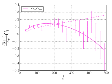
From the cross-correlation between the low- and high-richness samples, we expect a small or vanishing value of the effective objects per pixel density, because there is no overlap of objects between the two samples (except for systematic effects from cluster finding/identification and line of sight effects). However, the actual value of the effective pixel density is negative at the 2-$\sigma$ level. Again, this argues for strong exclusion effects between clusters of different richness (and thus halo mass), as observed in $N$-body simulations (Hamaus et al., 2010; Baldauf et al., 2013).

Figure 8 shows the measured angular power spectrum as well as the best-fit models using a vanishing shot-noise contribution (dashed line) and fitting for the shot-noise contribution (solid line). The measured $C_{l}$ show an unusual behavior as the correlation increases up to $l\approx 200$ and then decreases again. This cannot be described by a model with a vanishing (shown by the dashed line) shot-noise contribution, as a positive shot-noise contribution would worsen this mismatch. However, if allowing for negative non-Poissonian shot noise, the model yields a good description of the data. It will be interesting to see whether this measurement persists for larger sample sizes and other data sets.

Figure 8: Cross-correlation between the low- and high-richness samples described in Section 3. Lines indicate the best-fit models described in Sections 5.1 and 5.2: Dashed line shows the best-fit model specified in Equation (20), using a vanishing shot-noise contribution (as there is no overlap between the two samples), solid line represents the best-fit model specified in Equation (23), where $\bar{n}^{\rm eff}$ is added as a fit parameter to adjust the shot-noise contribution. The best fit $\bar{n}^{\rm eff}$ is negative in this case.

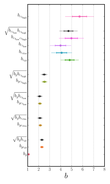
We have summarized the bias fit results for the different catalogue samples in Figure 9, which includes 1- and 2-sigma error bars for all measurements. This figure illustrates that the cross-check values (black symbols) and errors for bias from Equation (22) of the measurements of auto- and cross-correlations are consistent with each other for all measurements, including the volume-limited sample $c_{\rm vlim}$ as well as for the two richness bin samples $c_{\lambda_{\rm low}}$ and $c_{\lambda_{\rm high}}$.

Figure 9: The maximum likelihood galaxy and dark mater halo bias after marginalising over over $\bar{n}^{\rm eff}$, as well as the expectations denoted by $\sqrt{b_{a}b_{b}}$ from the cross-check described in Section 5.2. We also show $68\%$ (solid lines) and $95\%$ (faint solid lines) error bars.

6 Summary and Outlook

We have presented a first measurement of the cross-correlation angular power spectrum of galaxies and galaxy clusters using the SDSS DR8 galaxy and galaxy cluster sample. Further, we measured the auto- and cross-correlations of different sub-samples of the full cluster catalogue: a volume-limited sample as well as two samples of low and high richness.

We argued that in order to get a good theoretical description for the cross-correlation measurements we need to add an effective shot-noise contribution as an additional component to our model. Because there is some overlap of galaxies and galaxy clusters, we expect a non-vanishing shot-noise contribution. We find the measurements are much better described by a model containing sub-Poissonian shot noise and that using a regular Poisson shot noise correction results in an overcorrection. Since we also expect a deviation from Poissonian shot noise for cluster auto-correlations due to halo exclusion and non-linear clustering (Baldauf et al., 2013), we investigated if the cluster auto-correlation shows deviation from Poissonian shot noise as expected from simulations (Hamaus et al., 2010).

We extracted the effective bias for our measurements and used the results for the effective bias from auto-correlation measurements to perform a cross-check on the effective bias from the cross-correlation measurements. These cross-checks were in very good agreement after we allowed for non-Poissonian shot noise contribution. We performed the same cross-checks for measurements involving the subsamples of the cluster data and we find all measurements of effective bias to be consistent.

To compare our measurement of effective bias to theoretical expectations, we constructed a volume-limited cluster sample and found a relatively high value of $4.09\pm 0.47$ compared to our expectation of $b=2.8$. However, this value is consistent with previous measurements and supports the case for a fuller exploration of additional systematic effects, such as halo assembly bias.

Finally, we constructed a low and high richness sample from the full cluster sample and measured the auto- and cross-correlation as well. Again, the values for the effective bias are consistent with each other and are all relatively large for the cluster samples.

Most notably, we found a negative shot noise contribution for the cross-correlation at the 2-$\sigma$ level. This argues for strong exclusion effects between clusters of different richness (and thus halo mass), in agreement with $N$-body simulations. As larger and better data sets will become available, it will be interesting to see if this measurement of negative shot noise persists.

An appropriate treatment of shot noise is important for many other auto- and cross-correlation large scale structure analyses, i.e. different galaxy types and multi-tracer surveys. In the future, it will be essential to account for these effects to derive unbiased cosmology constraints from correlation functions and power spectra analyses.

References

- Abell (1958) Abell G. O., 1958, \hrefhttp://dx.doi.org/10.1086/190036 Astrophys.J.Suppl., \hrefhttp://adsabs.harvard.edu/abs/1958ApJS….3..211A 3, 211
- Aihara et al. (2011) Aihara H., et al., 2011, \hrefhttp://dx.doi.org/10.1088/0067-0049/193/2/29 Astrophys.J.Suppl., 193, 29
- Anderson et al. (2012) Anderson L., et al., 2012, \hrefhttp://dx.doi.org/10.1111/j.1365-2966.2012.22066.x MNRAS, \hrefhttp://adsabs.harvard.edu/abs/2012MNRAS.427.3435A 427, 3435
- Balaguera-Antolínez et al. (2011) Balaguera-Antolínez A., Sánchez A. G., Böhringer H., Collins C., Guzzo L., Phleps S., 2011, \hrefhttp://dx.doi.org/10.1111/j.1365-2966.2010.18143.x MNRAS, \hrefhttp://adsabs.harvard.edu/abs/2011MNRAS.413..386B 413, 386
- Baldauf et al. (2013) Baldauf T., Seljak U., Smith R. E., Hamaus N., Desjacques V., 2013, \hrefhttp://dx.doi.org/10.1103/PhysRevD.88.083507 PRD, \hrefhttp://adsabs.harvard.edu/abs/2013PhRvD..88h3507B 88, 083507
- Baxter et al. (2016) Baxter E. J., Rozo E., Jain B., Rykoff E., Wechsler R. H., 2016, preprint, \hrefhttp://adsabs.harvard.edu/abs/2016arXiv160400048B (\hrefhttp://arxiv.org/abs/1604.00048 arXiv:1604.00048)
- Bennett et al. (2013) Bennett C. L., et al., 2013, \hrefhttp://dx.doi.org/10.1088/0067-0049/208/2/20 ApJS, \hrefhttp://adsabs.harvard.edu/abs/2013ApJS..208…20B 208, 20
- Beutler et al. (2011) Beutler F., et al., 2011, \hrefhttp://dx.doi.org/10.1111/j.1365-2966.2011.19250.x MNRAS, \hrefhttp://adsabs.harvard.edu/abs/2011MNRAS.416.3017B 416, 3017
- Beutler et al. (2014) Beutler F., et al., 2014, \hrefhttp://dx.doi.org/10.1093/mnras/stu1051 MNRAS, \hrefhttp://adsabs.harvard.edu/abs/2014MNRAS.443.1065B 443, 1065
- Blake et al. (2011) Blake C., et al., 2011, \hrefhttp://dx.doi.org/10.1111/j.1365-2966.2011.19592.x MNRAS, \hrefhttp://adsabs.harvard.edu/abs/2011MNRAS.418.1707B 418, 1707
- Blas et al. (2011) Blas D., Lesgourgues J., Tram T., 2011, \hrefhttp://dx.doi.org/10.1088/1475-7516/2011/07/034 JCAP, \hrefhttp://adsabs.harvard.edu/abs/2011JCAP…07..034B 7, 034
- Challinor & Chon (2005) Challinor A., Chon G., 2005, \hrefhttp://dx.doi.org/10.1111/j.1365-2966.2005.09076.x MNRAS, \hrefhttp://adsabs.harvard.edu/abs/2005MNRAS.360..509C 360, 509
- Chon et al. (2004) Chon G., Challinor A., Prunet S., Hivon E., Szapudi I., 2004, \hrefhttp://dx.doi.org/10.1111/j.1365-2966.2004.07737.x Mon.Not.Roy.Astron.Soc., 350, 914
- Cole et al. (2005) Cole S., et al., 2005, \hrefhttp://dx.doi.org/10.1111/j.1365-2966.2005.09318.x Mon.Not.Roy.Astron.Soc., 362, 505
- Collins et al. (2000) Collins C., Guzzo L., Boehringer H., Schuecker P., Chincarini G., et al., 2000, \hrefhttp://dx.doi.org/10.1046/j.1365-8711.2000.03918.x Mon.Not.Roy.Astron.Soc., 319, 939
- Cooray & Sheth (2002) Cooray A., Sheth R., 2002, \hrefhttp://dx.doi.org/10.1016/S0370-1573(02)00276-4 Physics Reports, \hrefhttp://adsabs.harvard.edu/abs/2002PhR…372….1C 372, 1
- Croft et al. (1999) Croft R. A. C., Dalton G. B., Efstathiou G., 1999, \hrefhttp://dx.doi.org/10.1046/j.1365-8711.1999.02381.x MNRAS, \hrefhttp://adsabs.harvard.edu/abs/1999MNRAS.305..547C 305, 547
- Das et al. (2014) Das S., et al., 2014, \hrefhttp://dx.doi.org/10.1088/1475-7516/2014/04/014 JCAP, \hrefhttp://adsabs.harvard.edu/abs/2014JCAP…04..014D 4, 014
- Di Dio et al. (2013) Di Dio E., Montanari F., Lesgourgues J., Durrer R., 2013, \hrefhttp://dx.doi.org/10.1088/1475-7516/2013/11/044 JCAP, \hrefhttp://adsabs.harvard.edu/abs/2013JCAP…11..044D 11, 044
- Efstathiou (2004) Efstathiou G., 2004, \hrefhttp://dx.doi.org/10.1111/j.1365-2966.2004.07530.x MNRAS, \hrefhttp://adsabs.harvard.edu/abs/2004MNRAS.349..603E 349, 603
- Eisenstein et al. (2011) Eisenstein D. J., et al., 2011, \hrefhttp://dx.doi.org/10.1088/0004-6256/142/3/72 Astron.J., 142, 72
- Estrada et al. (2009) Estrada J., Sefusatti E., Frieman J. A., 2009, \hrefhttp://dx.doi.org/10.1088/0004-637X/692/1/265 Astrophys.J., 692, 265
- Farahi et al. (2016) Farahi A., Evrard A. E., Rozo E., Rykoff E. S., Wechsler R. H., 2016, preprint, \hrefhttp://adsabs.harvard.edu/abs/2016arXiv160105773F (\hrefhttp://arxiv.org/abs/1601.05773 arXiv:1601.05773)
- Fedeli et al. (2011) Fedeli C., Carbone C., Moscardini L., Cimatti A., 2011, \hrefhttp://dx.doi.org/10.1111/j.1365-2966.2011.18490.x MNRAS, \hrefhttp://adsabs.harvard.edu/abs/2011MNRAS.414.1545F 414, 1545
- Fry & Gaztanaga (1993) Fry J. N., Gaztanaga E., 1993, \hrefhttp://dx.doi.org/10.1086/173015 ApJ, \hrefhttp://adsabs.harvard.edu/abs/1993ApJ…413..447F 413, 447
- Gao & White (2007) Gao L., White S. D. M., 2007, \hrefhttp://dx.doi.org/10.1111/j.1745-3933.2007.00292.x MNRAS, \hrefhttp://adsabs.harvard.edu/abs/2007MNRAS.377L…5G 377, L5
- Gao et al. (2005) Gao L., Springel V., White S. D. M., 2005, \hrefhttp://dx.doi.org/10.1111/j.1745-3933.2005.00084.x MNRAS, \hrefhttp://adsabs.harvard.edu/abs/2005MNRAS.363L..66G 363, L66
- Giannantonio & Percival (2014) Giannantonio T., Percival W. J., 2014, \hrefhttp://dx.doi.org/10.1093/mnrasl/slu036 MNRAS, \hrefhttp://adsabs.harvard.edu/abs/2014MNRAS.441L..16G 441, L16
- Giannantonio et al. (2006) Giannantonio T., et al., 2006, \hrefhttp://dx.doi.org/10.1103/PhysRevD.74.063520 PRD, \hrefhttp://adsabs.harvard.edu/abs/2006PhRvD..74f3520G 74, 063520
- Giannantonio et al. (2012) Giannantonio T., Crittenden R., Nichol R., Ross A. J., 2012, \hrefhttp://dx.doi.org/10.1111/j.1365-2966.2012.21896.x Mon.Not.Roy.Astron.Soc., 426, 2581
- Giannantonio et al. (2016) Giannantonio T., Fosalba P., Cawthon R., Omori Y., Crocce M., et al., 2016, \hrefhttp://dx.doi.org/10.1093/mnras/stv2678 MNRAS, \hrefhttp://adsabs.harvard.edu/abs/2016MNRAS.456.3213G 456, 3213
- Gorski et al. (2005) Gorski K., Hivon E., Banday A., Wandelt B., Hansen F., et al., 2005, \hrefhttp://dx.doi.org/10.1086/427976 Astrophys.J., 622, 759
- Grieb et al. (2016) Grieb J. N., Sánchez A. G., Salazar-Albornoz S., Scoccimarro R., Crocce M., Dalla Vecchia C., et al. 2016, preprint, \hrefhttp://adsabs.harvard.edu/abs/2016arXiv160703143G (\hrefhttp://arxiv.org/abs/1607.03143 arXiv:1607.03143)
- Hamaus et al. (2010) Hamaus N., Seljak U., Desjacques V., Smith R. E., Baldauf T., 2010, \hrefhttp://dx.doi.org/10.1103/PhysRevD.82.043515 PRD, \hrefhttp://adsabs.harvard.edu/abs/2010PhRvD..82d3515H 82, 043515
- Hamaus et al. (2014) Hamaus N., Wandelt B. D., Sutter P. M., Lavaux G., Warren M. S., 2014, \hrefhttp://dx.doi.org/10.1103/PhysRevLett.112.041304 Physical Review Letters, \hrefhttp://adsabs.harvard.edu/abs/2014PhRvL.112d1304H 112, 041304
- Hamaus et al. (2016) Hamaus N., Pisani A., Sutter P. M., Lavaux G., Escoffier S., Wandelt B. D., Weller J., 2016, \hrefhttp://dx.doi.org/10.1103/PhysRevLett.117.091302 Physical Review Letters, \hrefhttp://adsabs.harvard.edu/abs/2016PhRvL.117i1302H 117, 091302
- Hartlap et al. (2007) Hartlap J., Simon P., Schneider P., 2007, \hrefhttp://dx.doi.org/10.1051/0004-6361:20066170 Astron. & Astrophys., \hrefhttp://adsabs.harvard.edu/abs/2007A
- Hayes et al. (2011) Hayes B., Brunner R., Ross A., 2011, preprint, \hrefhttp://adsabs.harvard.edu/abs/2011arXiv1112.5723H (\hrefhttp://arxiv.org/abs/1112.5723 arXiv:1112.5723)
- Ho et al. (2012) Ho S., Cuesta A., Seo H.-J., et al., 2012, \hrefhttp://dx.doi.org/10.1088/0004-637X/761/1/14 ApJ, \hrefhttp://adsabs.harvard.edu/abs/2012ApJ…761…14H 761, 14
- Huetsi (2009) Huetsi G., 2009
- Hütsi & Lahav (2008) Hütsi G., Lahav O., 2008, \hrefhttp://dx.doi.org/10.1051/0004-6361:200810250 Astron. & Astrophys., \hrefhttp://adsabs.harvard.edu/abs/2008A
- Johnson et al. (2016) Johnson A., Blake C., Dossett J., Koda J., Parkinson D., Joudaki S., 2016, \hrefhttp://dx.doi.org/10.1093/mnras/stw447 MNRAS, \hrefhttp://adsabs.harvard.edu/abs/2016MNRAS.458.2725J 458, 2725
- La Porta et al. (2008) La Porta L., Burigana C., Reich W., Reich P., 2008, \hrefhttp://dx.doi.org/10.1051/0004-6361:20078435 Astron. & Astrophys., \hrefhttp://adsabs.harvard.edu/abs/2008A
- Lilje & Efstathiou (1988) Lilje P. B., Efstathiou G., 1988, Mon.Not.Roy.Astron.Soc., \hrefhttp://adsabs.harvard.edu/abs/1988MNRAS.231..635L 231, 635
- Mana et al. (2013) Mana A., Giannantonio T., Weller J., Hoyle B., Huetsi G., et al., 2013, \hrefhttp://dx.doi.org/10.1093/mnras/stt1062 Mon.Not.Roy.Astron.Soc., 434, 684
- McDonald (2006) McDonald P., 2006, \hrefhttp://dx.doi.org/10.1103/PhysRevD.74.103512 PRD, \hrefhttp://adsabs.harvard.edu/abs/2006PhRvD..74j3512M 74, 103512
- Miyatake et al. (2016) Miyatake H., More S., Takada M., Spergel D. N., Mandelbaum R., Rykoff E. S., Rozo E., 2016, \hrefhttp://dx.doi.org/10.1103/PhysRevLett.116.041301 Physical Review Letters, \hrefhttp://adsabs.harvard.edu/abs/2016PhRvL.116d1301M 116, 041301
- More et al. (2016) More S., et al., 2016, \hrefhttp://dx.doi.org/10.3847/0004-637X/825/1/39 ApJ, \hrefhttp://adsabs.harvard.edu/abs/2016ApJ…825…39M 825, 39
- Padmanabhan et al. (2012) Padmanabhan N., Xu X., Eisenstein D. J., Scalzo R., Cuesta A. J., Mehta K. T., Kazin E., 2012, \hrefhttp://dx.doi.org/10.1111/j.1365-2966.2012.21888.x MNRAS, \hrefhttp://adsabs.harvard.edu/abs/2012MNRAS.427.2132P 427, 2132
- Peebles (1974) Peebles P. J. E., 1974, \hrefhttp://dx.doi.org/10.1086/190309 Astrophys.J.Suppl., \hrefhttp://adsabs.harvard.edu/abs/1974ApJS…28…37P 28, 37
- Percival et al. (2001) Percival W. J., et al., 2001, \hrefhttp://dx.doi.org/10.1046/j.1365-8711.2001.04827.x Mon.Not.Roy.Astron.Soc., 327, 1297
- Percival et al. (2010) Percival W. J., et al., 2010, \hrefhttp://dx.doi.org/10.1111/j.1365-2966.2009.15812.x MNRAS, \hrefhttp://adsabs.harvard.edu/abs/2010MNRAS.401.2148P 401, 2148
- Pillepich et al. (2012) Pillepich A., Porciani C., Reiprich T. H., 2012, \hrefhttp://dx.doi.org/10.1111/j.1365-2966.2012.20443.x MNRAS, \hrefhttp://adsabs.harvard.edu/abs/2012MNRAS.422…44P 422, 44
- Planck Collaboration et al. (2014) Planck Collaboration et al., 2014, \hrefhttp://dx.doi.org/10.1051/0004-6361/201321591 Astron. & Astrophys., \hrefhttp://adsabs.harvard.edu/abs/2014A
- Reichardt et al. (2012) Reichardt C. L., et al., 2012, \hrefhttp://dx.doi.org/10.1088/0004-637X/755/1/70 ApJ, \hrefhttp://adsabs.harvard.edu/abs/2012ApJ…755…70R 755, 70
- Ross et al. (2011) Ross A. J., Ho S., Cuesta A. J., Tojeiro R., Percival W. J., Wake D., Masters 2011, \hrefhttp://dx.doi.org/10.1111/j.1365-2966.2011.19351.x MNRAS, \hrefhttp://adsabs.harvard.edu/abs/2011MNRAS.417.1350R 417, 1350
- Rykoff et al. (2014) Rykoff E., et al., 2014, \hrefhttp://dx.doi.org/10.1088/0004-637X/785/2/104 Astrophys.J., 785, 104
- Sánchez et al. (2005) Sánchez A. G., Lambas D. G., Böhringer H., Schuecker P., 2005, \hrefhttp://dx.doi.org/10.1111/j.1365-2966.2005.09377.x MNRAS, \hrefhttp://adsabs.harvard.edu/abs/2005MNRAS.362.1225S 362, 1225
- Schlegel et al. (1998) Schlegel D. J., Finkbeiner D. P., Davis M., 1998, \hrefhttp://dx.doi.org/10.1086/305772 ApJ, \hrefhttp://adsabs.harvard.edu/abs/1998ApJ…500..525S 500, 525
- Schuecker et al. (2003) Schuecker P., Böhringer H., Collins C. A., Guzzo L., 2003, \hrefhttp://dx.doi.org/10.1051/0004-6361:20021715 Astron. & Astrophys., \hrefhttp://adsabs.harvard.edu/abs/2003A
- Seldner & Peebles (1977a) Seldner M., Peebles P. J. E., 1977a, \hrefhttp://dx.doi.org/10.1086/182428 Astrophys.J.Letters, \hrefhttp://adsabs.harvard.edu/abs/1977ApJ…214L…1S 214, L1
- Seldner & Peebles (1977b) Seldner M., Peebles P. J. E., 1977b, \hrefhttp://dx.doi.org/10.1086/155404 Astrophys.J., \hrefhttp://adsabs.harvard.edu/abs/1977ApJ…215..703S 215, 703
- Seldner et al. (1977) Seldner M., Siebers B., Groth E. J., Peebles P. J. E., 1977, \hrefhttp://dx.doi.org/10.1086/112039 Astronomical Journal, \hrefhttp://adsabs.harvard.edu/abs/1977AJ…..82..249S 82, 249
- Seljak (2000) Seljak U., 2000, \hrefhttp://dx.doi.org/10.1046/j.1365-8711.2000.03715.x MNRAS, \hrefhttp://adsabs.harvard.edu/abs/2000MNRAS.318..203S 318, 203
- Shane & Wirtanen (1967) Shane C. D., Wirtanen C. A., 1967, Publications of the Lick Observatory, 22, part 1
- Sheth & Tormen (2004) Sheth R. K., Tormen G., 2004, \hrefhttp://dx.doi.org/10.1111/j.1365-2966.2004.07733.x MNRAS, \hrefhttp://adsabs.harvard.edu/abs/2004MNRAS.350.1385S 350, 1385
- Simet et al. (2016) Simet M., McClintock T., Mandelbaum R., Rozo E., Rykoff E., Sheldon E., Wechsler R. H., 2016, preprint, \hrefhttp://adsabs.harvard.edu/abs/2016arXiv160306953S (\hrefhttp://arxiv.org/abs/1603.06953 arXiv:1603.06953)
- Smith et al. (2003) Smith R. E., et al., 2003, \hrefhttp://dx.doi.org/10.1046/j.1365-8711.2003.06503.x MNRAS, \hrefhttp://adsabs.harvard.edu/abs/2003MNRAS.341.1311S 341, 1311
- Szapudi et al. (2000) Szapudi I., Prunet S., Pogosyan D., Szalay A. S., Bond J. R., 2000
- Taylor et al. (2013) Taylor A., Joachimi B., Kitching T., 2013, \hrefhttp://dx.doi.org/10.1093/mnras/stt270 MNRAS, \hrefhttp://adsabs.harvard.edu/abs/2013MNRAS.432.1928T 432, 1928
- Tegmark et al. (2004) Tegmark M., et al., 2004, \hrefhttp://dx.doi.org/10.1103/PhysRevD.69.103501 Phys.Rev., D69, 103501
- Tinker et al. (2008) Tinker J., Kravtsov A. V., Klypin A., Abazajian K., Warren M., Yepes G., Gottlöber S., Holz D. E., 2008, \hrefhttp://dx.doi.org/10.1086/591439 ApJ, \hrefhttp://adsabs.harvard.edu/abs/2008ApJ…688..709T 688, 709
- Tinker et al. (2010) Tinker J. L., Robertson B. E., Kravtsov A. V., Klypin A., Warren M. S., Yepes G., Gottlöber S., 2010, \hrefhttp://dx.doi.org/10.1088/0004-637X/724/2/878 ApJ, \hrefhttp://adsabs.harvard.edu/abs/2010ApJ…724..878T 724, 878
- Veropalumbo et al. (2016) Veropalumbo A., Marulli F., Moscardini L., Moresco M., Cimatti A., 2016, \hrefhttp://dx.doi.org/10.1093/mnras/stw306 MNRAS, \hrefhttp://adsabs.harvard.edu/abs/2016MNRAS.458.1909V 458, 1909
- Wechsler et al. (2006) Wechsler R. H., Zentner A. R., Bullock J. S., Kravtsov A. V., Allgood B., 2006, \hrefhttp://dx.doi.org/10.1086/507120 ApJ, \hrefhttp://adsabs.harvard.edu/abs/2006ApJ…652…71W 652, 71
- York et al. (2000) York D. G., et al., 2000, \hrefhttp://dx.doi.org/10.1086/301513 AJ, \hrefhttp://adsabs.harvard.edu/abs/2000AJ….120.1579Y 120, 1579
- Zhao et al. (2013) Zhao G.-B., Saito S., Percival W. J., et al., 2013, \hrefhttp://dx.doi.org/10.1093/mnras/stt1710 MNRAS, \hrefhttp://adsabs.harvard.edu/abs/2013MNRAS.436.2038Z 436, 2038
- Zu & Weinberg (2013) Zu Y., Weinberg D. H., 2013, \hrefhttp://dx.doi.org/10.1093/mnras/stt411 MNRAS, \hrefhttp://adsabs.harvard.edu/abs/2013MNRAS.431.3319Z 431, 3319