Bergman et al.

On the Minimum Chordal Completion Polytope

On the Minimum Chordal Completion Polytope

David Bergman Operations and Information Management, University of Connecticut, Storrs, Connecticut 06260
david.bergman@business.uconn.edu

Carlos H. Cardonha IBM Research, Brazil, São Paulo 04007-900
carloscardonha@br.ibm.com

Andre A. Cire Department of Management, University of Toronto Scarborough, Toronto, Ontario M1C-1A4, Canada,
acire@utsc.utoronto.ca

Arvind U. Raghunathan Mitsubishi Electric Research Labs, 201 Broadway, Cambridge,
raghunathan@merl.com

A graph is chordal if every cycle of length at least four contains a chord, that is, an edge connecting two nonconsecutive vertices of the cycle. Several classical applications in sparse linear systems, database management, computer vision, and semidefinite programming can be reduced to finding the minimum number of edges to add to a graph so that it becomes chordal, known as the minimum chordal completion problem (MCCP). In this article we propose a new formulation for the MCCP which does not rely on finding perfect elimination orderings of the graph, as has been considered in previous work. We introduce several families of facet-defining inequalities for cycle subgraphs and investigate the underlying separation problems, showing that some key inequalities are NP-Hard to separate. We also show general properties of the proposed polyhedra, indicating certain conditions and methods through which facets and inequalities associated with the polytope of a certain graph can be adapted in order to become valid and eventually facet-defining for some of its subgraphs or supergraphs. Numerical studies combining heuristic separation methods based on a threshold rounding and lazy-constraint generation indicate that our approach substantially outperforms existing methods for the MCCP, solving many benchmark graphs to optimality for the first time.

Networks/graphs; Applications: Networks/graphs ; Programming: Integer: Algorithms: Cutting plane/facet

1 Introduction

Given a simple undirected graph $G=(V,E)$, the minimum chordal completion problem (MCCP) asks for the minimum number of edges to add to $E$ so that the graph becomes chordal; that is, every cycle of length at least four in $G$ has an edge connecting two non-consecutive vertices (i.e., a chord). Figure 1(b) depicts an example of a minimum chordal completion of the graph in Figure 1(a), where a chord $\{v_{1},v_{3}\}$ is added because of the chordless cycle $(v_{0},v_{1},v_{4},v_{3})$. The problem is also referred to as the minimum triangulation problem or the minimum fill-in problem.

The MCCP is a classical combinatorial optimization problem with a variety of applications spanning both the computer science and the operations research literature. Initial algorithmic aspects for directed graphs were investigated by Rose et al. (1976) and Rose and Tarjan (1978), motivated by problems arising in Gaussian elimination of sparse linear equality systems. The most general version of the MCCP was only proven NP-Hard later by Yannakakis (1981), and since then minimum graph chordalization methods have been applied in database management (Beeri et al. 1983, Tarjan and Yannakakis 1984), sparse matrix computation (Grone et al. 1984, Fomin et al. 2013), artificial intelligence (Lauritzen and Spiegelhalter 1990), computer vision (Chung and Mumford 1994), and in several other contexts; see, e.g., the survey by Heggernes (2006). Most recently, solution methods for the MCCP have gained a central role in semidefinite and nonlinear optimization, in particular for exploiting sparsity of linear and nonlinear constraint matrices (Nakata et al. 2003, Kim et al. 2011, Vandenberghe and Andersen 2015).

Figure 1: (a) An example graph by Heggernes (2006). (b) A minimum chordal completion of the graph. (c) A minimal, non-optimal chordal completion of the graph.

The literature on exact computational approaches for the MCCP is, however, surprisingly scarce. A large stream of research in the computer science community has focused on the identification of polynomial-time algorithms for structured classes of graphs, such as the works by Chang (1996), Broersma et al. (1997), Kloks et al. (1998), and Bodlaender et al. (1998). For general graphs, Kaplan et al. (1999) proposed the first exact fixed-parameter tractable algorithm for the MCCP, and recently Fomin and Villanger (2012) presented a substantially faster procedure with sub-exponential parameterized time complexity. Such algorithms are typically extremely challenging to implement and have not been used in computational experiments involving existing datasets.

In regards to practical optimization approaches, the primary focus has been on heuristic methodologies with no optimality guarantees, including techniques by Mezzini and Moscarini (2010), Rollon and Larrosa (2011), and Berry et al. (2006, 2003). The state-of-the-art heuristic, proposed by George and Liu (1989), is a simple and efficient algorithm based on ordering the vertices by their degree. Previous articles have also developed methodologies for finding a minimal chordal completion. Note that a minimal chordal completion is not necessarily minimum, as depicted in Figure 1(c), but does provide a heuristic solution to the MCCP.

To the best of our knowledge, the first mathematical programming model for the MCCP is derived from a simple modification of the formulation by Feremans et al. (2002) for determining the tree-widths of graphs. The model is based on a result by Fulkerson and Gross (1965), which states that a graph is chordal if and only it has a perfect elimination ordering, to be detailed further in this paper. Yüceoğlu (2015) has recently provided a first polyhedral analysis and computational testing of this formulation, deriving facets and other valid inequalities for specific classes of graphs. Alternatively, Bergman and Raghunathan (2015) introduced a Benders approach to the MCCP that relies on a simple class of valid inequalities, outperforming a simple constraint programming backtracking search algorithm.

Our Contributions

In this paper we investigate a novel computational approach to the MCCP that extends the preliminary work of Bergman and Raghunathan (2015). Our technique is based on a mathematical programming model composed of exponentially many constraints – the chordal inequalities – that are defined directly on the edge space of the graph and do not depend on the perfect elimination ordering property, as opposed to earlier formulations. We investigate the polyhedral structure of our model, which reveals that the proposed inequalities are part of a special class of constraints that induce exponentially many facets for cycle subgraphs. This technique can be generalized to lift other inequalities and greatly strengthen the corresponding linear programming relaxation.

Building on these theoretical results, we propose a hybrid solution method that alternates a lazy-constraint generation with a heuristic separation procedure. The resulting approach is compared to the current state-of-the-art models in the literature, and it is empirically shown to improve solution times and known optimality gaps for standard graph benchmarks, often by orders of magnitude.

Organization of the Paper.

After introducing our notation in §2, in §3 we describe a new integer programming (IP) formulation for the MCCP and characterize its polytope in §4, also proving dimensionality results and simple upper bound facets. §5 provides an in-depth analysis of the polyhedral structure of cycle graphs, introducing four classes of facet-defining inequalities. In §6 we prove general properties of the polytope, including some results relating to the lifting of facets. Finally, in §7 we propose a hybrid solution technique that considers both a lazy-constraint generation and a heuristic separation method based on a threshold rounding procedure, and also present a simple primal heuristic for the problem. We provide a numerical study in §8, indicating that our approach substantially outperforms existing methods, in particular solving many benchmark graphs to optimality for the first time.

2 Notation and Terminology

For the remainder of the paper, we assume that each graph $G=(V,E)$ is connected, undirected, and does not contain self-loops or multi-edges. For any set $S$, ${{S}\choose{2}}$ denotes the family of two-element subsets of $S$. Each edge $e\in E\subseteq{V\choose 2}$ is a two-element subset of vertices in $V$. The complement edge set (or fill edges) $E^{c}$ of $G$ is the set of edges missing from $G$, that is, $E^{c}={V\choose 2}\backslash E$. We denote by $m$ and $m^{c}$ the cardinality of the edge set and of the complement edge set of $G$, respectively (i.e., $m=|E|$ and $m^{c}=|E^{c}|$). The graph induced by a set $V^{\prime}\subseteq V$ is the graph $G[V^{\prime}]=\left(V^{\prime},E^{\prime}\right)$ whose edge set is such that $E^{\prime}=E\cap{V^{\prime}\choose 2}$. If multiple graphs are being considered in a context, we include “$(G)$” in the notation to avoid ambiguity; i.e., $V(G^{\prime})$ and $E(G^{\prime})$ represent the vertex and edge set of a graph $G^{\prime}$, respectively. Moreover, for every integer $k\geq 0$, we let $[k]:=\{1,2,\ldots,k\}$.

For any ordered list $C=(v_{0},v_{1},\ldots,v_{k-1})$ of $k$ distinct vertices of $V$, let $V(C)=\{v_{0},v_{1},\ldots,v_{k-1}\}$ be the set of vertices composing $C$ and let $|V(C)|$ be the size $|C|$ of $C$. The exterior of $C$ is the family

$$\textnormal{ext}(C)=\{\{v_{k-1},v_{0}\}\}\cup\bigcup_{i\in[k-1]}\{\{v_{i-1},v_{i}\}\},$$

and the interior of $C$ is the family of two-element subsets of $V(C)$ that do not belong to $\textnormal{ext}(C)$, that is,

$$\textnormal{int}(C)={V(C)\choose 2}\setminus\textnormal{ext}(C).$$

We call $C$ a cycle if $\textnormal{ext}(C)\subseteq E$. If $C$ is a cycle, any element of $\textnormal{int}(C)$ is referred to as a chord. A cycle $C$ for which the induced graph $G[V(C)]$ contains no chords is a chordless cycle. $G$ is said to be chordal if the maximum size of any chordless cycle is three. A chordless cycle with $k$ vertices is called a $k$-chordless cycle.

Let $G=(V,E)$. Every subset of fill edges $F\subseteq E^{c}$ is a completion of $G$, and $G+F$ represents the graph that results from the addition of edges in $F$ to $E$; that is, $G+F:=(V,E\cup F)$. A chordal completion of $G$ is any subset of fill edges $F\subseteq E^{c}$ for which the completion $G+F$ is chordal. A minimal chordal completion $F$ is a chordal completion such that, for any proper subset $F^{\prime}\subset F$, $F^{\prime}$ is not a chordal completion for $G$. A minimum chordal completion is a minimal chordal completion of minimum cardinality, and the minimum chordal completion problem (MCCP) is about the identification of such a subset of $E^{c}$.

Example 2.1

Consider the graph in Figure 1(a). This graph has three chordless cycles, $C_{1}=(v_{0},v_{1},v_{2},v_{3})$, $C_{2}=(v_{1},v_{2},v_{3},v_{4})$ and $C_{3}=(v_{0},v_{1},v_{4},v_{3})$. Figure 1(c) shows a chordal completion consisting of edges $\{v_{0},v_{2}\},\{v_{2},v_{4}\}$, and $\{v_{0},v_{4}\}$. Removing any of these edges will result in a graph that is not chordal, so this chordal completion is minimal. Figure 1(b) shows a smaller minimal chordal completion, a minimum chordal completion consisting only of edge $\{v_{1},v_{3}\}$.

3 IP Formulation for the MCCP

We now describe the basic IP formulation investigated in this paper. Given a graph $G=(V,E)$, each binary variable $x_{f}$ in our model indicates whether the fill edge $f\in E^{c}$ is part of a chordal completion for $G$. That is, if we define the set $E(x):=\left\{f\in E^{c}:x_{f}=1\right\}$ for each vector $x\in[0,1]^{m^{c}}$, the set of feasible solutions to our model is given by

$$X(G):=\left\{x\in\{0,1\}^{m^{c}}:G+E(x)\;\;\textnormal{is chordal}\right\}.$$

Thus, each $x\in X(G)$ equivalently represents the characteristic vector of a chordal completion of $G$. We use $G(x)$ to denote $G+E(x)$, i.e., $G(X)=(V,E\cup E(x))$, and $x(F)$ to represent the characteristic vector of completion $F\subseteq E^{c}$, i.e., $x(F)_{f}=1$ if $f\in F$ and $x(F)_{f}=0$ otherwise.

Let $\mathcal{C}$ be the family of all possible ordered lists composed of distinct vertices of $V$, i.e., every $C\in\mathcal{C}$ can be written as a sequence $C=(v_{0},v_{1},\dots,v_{k-1})$ for some $k\leq|V|$. Also, let $F_{G}(C)=F(C)\subseteq E^{c}$ be the set of fill edges that are missing in $\textnormal{ext}(C)$ for $C$ to induce a cycle in $G$, that is,

$$F(C):=\textnormal{ext}(C)\setminus E.$$

We propose the following model for the MCCP:

minimize $$\sum_{f\in E^{c}}x_{f}$$ (IPC)

s.t. $$\sum_{f\in\textnormal{int}(C)}x_{f}-(|C|-3)\left(\sum_{f\in F(C)}x_{f}-|F(C)|+1\right)\geq 0,\;\;\textnormal{for all $C\in\mathcal{C}$},$$ (I1)

with $$\textnormal{int}(C)\cap E=\emptyset$$

$$x\in\{0,1\}^{m^{c}}.$$

The set of inequalities (I1) will be denoted by chordal inequalities henceforth. Note that every sequence $C$ such that $F(C)=\emptyset$ and $\textnormal{int}(C)\cap E=\emptyset$ describes a cycle in $G$, and its associated inequality (I1) simplifies to

$$\sum_{f\in\textnormal{int}(C)}x_{f}\geq|C|-3.$$

Lemma 3.1 shows that inequalities (I1) are valid in this special case.

Lemma 3.1

If $C$ is a chordless cycle of $G$ such that $|C|\geq 4$, then any chordal completion of $G$ contains at least $|C|-3$ edges that belong to $\textnormal{int}(C)$.

Proof 3.2

Proof. We proceed by induction on $k$, the cardinality of sequence $C=(v_{0},v_{1},\ldots,v_{k-1})$. For $k=4$, if fewer than $4-3=1$ edges (i.e., 0 edges) belonging to $\textnormal{int}(C)$ are added to $G$, the graph trivially remains not chordal. Assume now $k\geq 5$. By definition, any chordless completion of $G$ must contain at least one edge in $\textnormal{int}(C)$, so let us suppose without loss of generality that a chord $\left\{v_{0},v_{p}\right\}$ is added to $G$ for some $1<p<k-1$.

If $p=2$ (or $p=k-2$), then $C^{\prime}=(v_{0},v_{2},\ldots,v_{k-1})$ is a chordless cycle of length $k-1$. By the inductive hypothesis, any chordal completion requires at least $(k-1)-3=k-4$ edges in $\textnormal{int}(C^{\prime})$ (which are also in $\textnormal{int}(C)$). By symmetry, the same analysis and result hold if $p=k-2$. Therefore any chordal completion of $G$ employing chord $\left\{v_{0},v_{p}\right\}$ for $p=2$ (or $p=k-2$) requires at least $1+k-4=k-3$ edges in $\textnormal{int}(C)$.

Finally, let $3\leq p\leq k-3$. In this case, chord $\left\{v_{0},v_{p}\right\}$ cuts $C$ and creates two chordless cycles: $C^{1}=(v_{0},v_{1},\ldots,v_{p})$ and $C^{2}=(v_{0},v_{p},v_{p+1},\ldots,v_{k-1})$. By the inductive hypothesis, any chordless completion of $G$ requires at least $p-3$ edges in $\textnormal{int}(C^{1})$ and at least $k-p+2-3=k-p-1$ edges in $\textnormal{int}(C^{2})$; as $\textnormal{int}(C^{1})\cap\textnormal{int}(C^{2})=\emptyset$ and $\textnormal{int}(C^{1})\cup\textnormal{int}(C^{2})\subset\textnormal{int}(C)$, any chordal completion of $G$ employing chord $\left\{1,v_{p}\right\}$ for $3\leq p\leq k-3$ also requires at least $(1)+(p-3)+(k-p-1)=k-3$ edges in $\textnormal{int}(C)$, as desired.

Based on the previous lemma, we show below that the set of inequalities (I1) is valid for all sequences in $\mathcal{C}$ and, as a consequence, that (IPC) is a valid formulation for the MCCP.

Proposition 3.3

The model (IPC) is a valid formulation for the MCCP.

Proof 3.4

Proof. We first show that there is an one-to-one correspondence between $X(G)$ and solutions to (IPC). Let $x^{*}$ be a feasible solution to (IPC) and suppose that the graph $G+E(x^{*})$ contains a chordless cycle $C$ with more than 3 vertices. By definition, $\sum_{f\in\textnormal{int}(C)}x^{*}_{f}=0<|C|-3$, thus contradicting the feasibility of $x^{*}$. Conversely, let $E^{*}\subseteq E^{c}$ be such that $G+E^{*}$ is chordal, and suppose $x^{*}=\{x\in\{0,1\}^{m^{c}}:x_{f}=1\Leftrightarrow f\in E^{*}\}$ is infeasible to (IPC). Assume that one of the violated inequalities is associated with sequence $C^{*}$; note that $\sum_{f\in F(C^{*})}x_{f}=|F(C^{*})|$, as the associated inequality would be trivially satisfied otherwise. Therefore, $C^{*}$ is a cycle in $G+E^{*}$ and we must have $\sum_{f\in\textnormal{int}(C^{*})}x_{f}<|C|-3$, which, by Lemma 3.1, contradicts the fact that $G+E^{*}$ is chordal. Finally, since the one-to-one correspondence holds and the objective function of (IPC) minimizes the number of added edges, the result follows.

4 MCCP Polytope Dimension and Simple Upper Bound Facets

This section begins our investigation of the convex hull of the feasible set of chordal completions $X(G)$, which will lead to special properties that can be exploited by computational methods for the MCCP. We identify the dimension of the polytope and provide a proof that the simple upper bound inequalities $x_{f}\leq 1$ are facet-defining.

Theorem 4.1

If $G=(V,E)$ is not a complete graph (and hence not trivially chordal),

    a. $\textnormal{conv}(X(G))$ is full-dimensional;

    b. $x_{f}\leq 1$ is facet-defining for all $f\in E^{c}$.

Proof 4.2

Proof. We first show (a). Let $e\in\{0,1\}^{m^{c}}$ be the vector consisting only of ones and $e^{j}\in\{0,1\}^{m^{c}}$ be the unit vector for coordinate $j$. By definition, $G+E(e)$ is the complete graph (which is trivially chordal), whereas $G+E(e-e^{j})$ is the complete graph with only the edge associated with coordinate $j$ missing. Graphs $G+E(e-e^{j})$ are chordal for every $e^{j}$; this follows because the graph induced by the set of vertices in any cycle $C$ of cardinality $k\geq 4$ contains at least ${k\choose 2}-1$ edges and, consequently, $|\textnormal{int}(C)|\geq{k\choose 2}-1-k=\frac{k^{2}-3k-2}{2}$, which is greater than or equal to 1 for $k\geq 4$. The set of $m^{c}+1$ vectors $\{e\}\cup\{e-e^{1},e-e^{2},\ldots,e-e^{m^{c}}\}$ is affinely independent and contained in the set $X(G)$, and so it follows that $\textnormal{conv}(X(G))$ is a full-dimensional polytope.

For $(b)$, let $f\in E^{c}$ and notice that the set of $m^{c}$ vectors $\{e\}\cup\{e-e^{f^{\prime}}:f^{\prime}\in E^{c}\setminus\{f\}\}$ is affinely independent and satisfy $x_{f}=1$.

5 Cycle Graph Facets

We restrict our attention now to cycle graphs, i.e., graphs consisting of a single cycle. Cycle graphs are the building blocks of computational methodologies for the MCCP, since finding a chordal completion of a graph naturally concerns identifying chordless cycles and eliminating them by adding chords. We present four classes of facet-defining inequalities for cycle graphs in this section.

Let $G=(V,E)$ be a cycle graph associated with a $k$-vertex chordless cycle $C=(v_{0},\dots,v_{k-1})$, i.e., $V=V(C)$ and $E=\textnormal{ext}(C)$. Assume all additions and subtractions involving indices of vertices are modulo-$k$. The proofs presented in this section show only the validity of the inequalities; arguments proving that they are facet-defining for cycle graphs are presented in Section 10.

Proposition 5.1

Let $G=(V,E)$ be a cycle graph associated with cycle $C=(v_{0},\dots,v_{k-1})$, $k\geq 4$. The chordal inequality (I1) associated with $C$, which in this case simplifies to

$$\sum_{f\in\textnormal{int}(C)}x_{f}\geq|C|-3,$$

is facet-defining for $\textnormal{conv}(X(G))$.

The proof of the validity of the inequality in Proposition 5.1 follows directly from Lemma 3.1.

Proposition 5.2

If $k\geq 4$, the inequality

$$x_{\{v_{i-1},v_{i+1}\}}+\sum_{f:v_{i}\in f,\{v_{i-1},v_{i+1}\}\cap f=\emptyset}x_{f}\geq\>1,\quad\;\textnormal{for all $i\in\{1,\dots,k\}$}$$ (I2)

is valid and facet-defining for $\textnormal{conv}(X(G))$.

Proof 5.3

Proof. Suppose that (I2) is violated by some $x\in\textnormal{conv}(X(G))$, i.e., that for some $\{v_{i-1},v_{i},v_{i+1}\}\subset V$, $x_{\{v_{i-1},v_{i+1}\}}+\sum_{f:v_{i}\in f,\{v_{i-1},v_{i+1}\}\cap f=\emptyset}x_{f}=0$. As $k\geq 4$, a shortest path $P$ from $v_{i-1}$ to $v_{i+1}$ in $G(x)$ that does not include $v_{i}$ traverses at least two edges. The sequence defined by the concatenation of $P$ with $(v_{i-1},v_{i},v_{i+1})$ defines thus a $k^{\prime}$-chordless cycle of $G(x)$ for $k^{\prime}\geq 4$, a contradiction.

For the next proposition, some additional notation is in order. For any two vertices $v_{i}$ and $v_{j}$ with $i<j$, let $d_{C}(v_{i},v_{j}):=\min\{j-i,k-j+i\}$ be the “distance” between $v_{i}$ and $v_{j}$ in $C$, and assume $d_{C}(v_{i},v_{j}):=d_{C}(v_{j},v_{i})$ if $i>j$.

Proposition 5.4

If $k\geq 5$, the inequality

$$\sum_{f\in\left\{\{v_{i},v_{j}\}\in E^{c}\,:\,d_{C}(v_{i},v_{j})=2\right\}}x_{f}\geq\>2$$ (I3)

is valid and facet-defining for $\textnormal{conv}(X(G))$.

Proof 5.5

Proof.

Inequality (I3) states that at least two out of the $|C|$ pairs of vertices of distance 2 must appear in any chordal completion of $G$. Without loss of generality, let $f^{\prime}=\{v_{0},v_{j_{1}}\}$ be the edge of $\textnormal{int}(C)$ composing some completion $F$ of $G$ that connects the “closest” vertices with respect to $d_{C}$. If $j_{1}\geq 3$, then $C^{\prime}=(v_{0},v_{1},\ldots,v_{j_{1}})$ is a chordless cycle in $G+F$, a contradiction; therefore, $j_{1}=2$.

As $k\geq 5$, $C^{\prime}=(v_{0},v_{2},v_{3},\ldots,v_{k-1})$ is a chordless cycle in $G+F$ with at least 4 vertices, so at least one edge of $\mathrm{int}(C^{\prime})$ must be present in $G+F$. Let $f^{\prime\prime}=\{v^{\prime}_{i},v^{\prime}_{j_{2}}\}$ be the edge of $\textnormal{int}(C^{\prime})$ that connects the “closest” vertices with respect to $d_{C^{\prime}}$. An argument similar to the one used above shows that $f^{\prime\prime}$ connects two vertices of distance 2 in $C^{\prime}$, so we have two cases to analyse. First, if $f^{\prime\prime}\neq\{v_{0},v_{2}\}$, the result follows directly. Otherwise, we either have $|C^{\prime}|=4$, in which case $d_{C^{\prime}}(v_{0},v_{2})=d_{C}(v_{0},v_{2})=2$, as desired, or we have a chordless cycle $C^{\prime\prime}=(v_{0},v_{3},\ldots,v_{k-1})$ in $G+F$ with at least 4 vertices, on which we can apply the same arguments; as an eventual sequence of cycles emerging from this construction will eventually lead to a cycle of length $4$, the result holds.

Proposition 5.6

If $k\geq 5$, the inequality

$$\sum_{f\in\textnormal{int}(C)\>\backslash\>\left\{\left\{v_{j-1},v_{j+1}\right\},\left\{v_{j},v_{i}\right\}\right\}}x_{f}\geq|C|-4,\quad\textnormal{for all}\;i,j\in\{1,\dots,k\},d_{C}(\{v_{j},v_{i}\})\geq 2$$ (I4)

is valid and facet defining for $\textnormal{conv}(X(G))$.

Proof 5.7

Proof. Given vertices $v_{i}$ and $v_{j}$ such that $d_{C}(\{v_{j},v_{i}\})\geq 2$, inequality (I4) enforces the inclusion of at least $|C|-4$ edges of $\textnormal{int}(C)\setminus\{\{v_{j-1},v_{j+1}\},\{v_{j},v_{i}\}\}$ in any chordal completion of $G$. Without loss of generality, let $j=0$ and let $i$ be any value in $[2,k-3]$. Suppose by contradiction that there exists $x^{0}\in X(G)$ such that

$$\sum_{f\in\textnormal{int}(C)\>\backslash\>\left\{\left\{v_{k-1},v_{1}\right\},\left\{v_{0},v_{i}\right\}\right\}}x^{0}_{f}<|C|-4.$$ (1)

By Lemma 3.1, we have that

$$\sum_{f\in\textnormal{int}(C)}x^{0}_{f}\geq|C|-3.$$

This implies that $x^{0}_{v_{k-1},v_{1}}=x^{0}_{v_{0},v_{i}}=1$, for otherwise inequality 1 would be violated. Thus, the sequences $C^{1}=\left(v_{0},v_{1},\ldots,v_{i}\right)$ and $C^{2}=\left(v_{0},v_{i},v_{i+1},\ldots,v_{k-1}\right)$ are cycles in $G(x^{0})$. Again, by Lemma 3.1, at least $\left|C^{\ell}\right|-3$ fill edges must be present in $\textnormal{int}(C^{\ell})$, $\ell=1,2$. This is only possible if at least $i-2$ edges of $\textnormal{int}(C^{1})$ and at least $|C|-i-2$ edges of $\textnormal{int}(C^{2})$ belong to the set of fill edges described by $x^{0}$. As $\textnormal{int}(C^{1})\cap\textnormal{int}(C^{2})=\emptyset$ and $\textnormal{int}(C^{1})\cup\textnormal{int}(C^{2})\subseteq\textnormal{int}(C)$, we have that

$$\sum_{f\in\textnormal{int}(C)\>\backslash\>\left\{\left\{v_{i-1},v_{i+1}\right\},\left\{v_{0},v_{i}\right\}\right\}}x^{0}_{f}\geq\sum_{f\in\mathrm{int}(C^{1})}x^{0}_{f}+\sum_{f\in\mathrm{int}(C^{2})}x^{0}_{f}\geq|C|-4,$$

contradicting thus inequality (1).

Example 5.8

Let $G$ be a cycle graph associated with 6-cycle $C=(v_{0},v_{1},v_{2},v_{3},v_{4},v_{5})$. An example of inequality (I2) with $i=1$ is

$$x_{\{v_{0},v_{2}\}}+\left(x_{\{v_{1},v_{3}\}}+x_{\{v_{1},v_{4}\}}+x_{\{v_{1},v_{5}\}}\right)\geq 1,$$

which enforces the inclusion of at least one edge $f=\{v_{1},v_{k}\}$, $k\in\{3,4,5\}$, for every chordal completion of $G$ that does not contain edge $(v_{0},v_{2})$.

Inequality (I3) translates to

$$x_{\{v_{5},v_{1}\}}+x_{\{v_{0},v_{2}\}}+x_{\{v_{1},v_{3}\}}+x_{\{v_{2},v_{4}\}}+x_{\{v_{3},v_{5}\}}+x_{\{v_{4},v_{0}\}}\geq 2,$$

which enforces that at least 2 of the 6 pairs of vertices that are separated by one vertex must appear in any chordal completion of $G$.

Finally, inequality (I4) for $i=4$ and $j=1$ is given by

$$x_{\{v_{0},v_{3}\}}+x_{\{v_{0},v_{4}\}}+x_{\{v_{1},v_{3}\}}+x_{\{v_{1},v_{5}\}}+x_{\{v_{2},v_{4}\}}+x_{\{v_{2},v_{5}\}}+x_{\{v_{3},v_{5}\}}\geq 2,$$

which enforces that at least 2 of the edges in $\textnormal{int}(C)\setminus\{\{v_{0},v_{2}\},\{v_{1},v_{4}\}\}$ must be included in any chordal completion of $G$.

6 General Polyhedral Properties

This section provides theoretical insights into the polyhedral structure of the MCCP polytope. In particular, the first result, provided in Theorem 6.3, shows that any inequality proven to be valid on an induced subgraph can be extended into a valid inequality for the original graph. This result is important for the development of practical solution methodology because it shows that finding valid inequalities/facets on particular substructures, such as cycles, can help in the generation of valid inequalities for larger graphs containing these substructures. Theorem 6.5 shows how facets for cycles can be lifted to facets of graphs that are subgraphs of cycles, leading to the result in Corollary 6.6 relating to when the inequalities (I1) in their general form in model (IPC) are facet-defining. The final result of the section, Theorem 6.8, proves and describes how facets for small cycles can be lifted to facets of larger cycles.

First, we show a lemma that will be used in the proof of Theorem 6.3.

Lemma 6.1

If $G=(V,E)$ is chordal, then $G[W]$ is chordal for any $W\subseteq V$.

Proof 6.2

Proof. A chordless cycle $C$ in $G[W]$ must be a chordless cycle in $G$. Thus, if $G[W]$ is not chordal, then $G$ cannot be as well. $\Halmos$

Theorem 6.3

Let $G=(V,E)$ be an arbitrary graph and $W\subseteq V$ be any subset of vertices. If $a^{\prime}x^{\prime}\geq b$ is a valid inequality for $X(G[W])$, then $ax\geq b$ is a valid inequality for $X(G)$, where $a_{f}=a^{\prime}_{f}$ if $f\in E^{C}(G[W])$ and $a_{f}=0$ otherwise.

Proof 6.4

Proof. By way of contradiction, suppose that $a^{\prime}x^{\prime}\geq b$ is valid for $X(G[W])$ and let $F$ be a chordal completion of $G$ such that $ax(F)<b$. From the construction of $a$, we have $ax(F)=a^{\prime}x(F\cap E(G[W]))<b$, and by Lemma 6.1, $G[W]+F\cap E(G[W])$ must be chordal and, consequently, we must have $a^{\prime}x(F\cap E(G[W]))\geq b$, establishing thus a contradiction. $\Halmos$

We now present a result that goes in the opposite direction of Theorem 6.3. Namely, it shows how facet-defining inequalities for a cycle graph $G$ can be transformed into facet-defining inequalities for subgraphs of $G$; note that subgraphs of cycle graphs consist of collections of paths. This result allows us to show that inequality (I1) is facet-defining for subgraphs of cycle graphs.

Theorem 6.5

Let $G^{\prime}=(V,E^{\prime})$ be a cycle graph associated with the cycle $C=(v_{0},v_{1},\ldots,v_{k-1})\in\mathcal{C}$ and $G=(V,E)$ be a subgraph of $G^{\prime}$ such that $G^{\prime}=G+F_{G}(C),$ $F_{G}(C)=E^{\prime}\setminus E$. If $ax\geq b$ is facet-defining for $\textnormal{conv}(X(G^{\prime}))$, $a\geq\textbf{0}$, and $a^{\prime}\in\mathbb{R}^{|E^{C}|}$, with $a^{\prime}_{f}=a_{f}$ if $f\in E^{C}\setminus F_{G}(C)$ and $a^{\prime}_{f}=0$ otherwise, the inequality

$$a^{\prime}x\geq b\left(\sum_{f\in F_{G}(C)}x_{f}-|F_{G}(C)|+1\right)$$

is facet-defining for $\textnormal{conv}(X(G))$.

Figure 2: (a) A graph $G$ with $V=\{v_{0},v_{1},v_{2},v_{3},v_{4}\}$ and $E=\left\{\{v_{0},v_{1}\},\{v_{3},v_{4}\}\right\}$. Solid lines represent graph edges and dashed lines are fill edges whose addition to $G$ makes a chordal cycle of length 5. (b) Cycle graph with 5 vertices.

Theorem 6.5 (proved in Section LABEL:ec:generalProperties) immediately leads to the following result:

Corollary 6.6

For any graph $G=(V,E)$ and for any sequence $C\in\mathcal{C}$ such that $\textnormal{int}(C)\cap E=\emptyset$, the chordal inequality (I1) is facet-defining for the MCCP polytope of $G[V(C)]$.

Example 6.7

Consider the graph $G$ in Figure 2(a); solid lines represent graph edges in this example. As in the statement of Theorem 6.5, we have

$$C=\left(v_{0},v_{1},v_{2},v_{3},v_{4}\right),\;E(G)=\left\{\{v_{0},v_{1}\},\{v_{3},v_{4}\}\right\},\;\textnormal{and}\;F_{G}(C)=\left\{\{v_{1},v_{2}\},\{v_{2},v_{3}\},\{v_{4},v_{0}\}\right\}.$$

Graph $G+F(C)$ is 5-chordless cycle. One facet-defining inequality for this cycle, according to Proposition 5.1, is the simplified version of the chordal inequality, given by

$$x_{\{v_{0},v_{2}\}}+x_{\{v_{0},v_{3}\}}+x_{\{v_{1},v_{3}\}}+x_{\{v_{1},v_{4}\}}+x_{\{v_{2},v_{4}\}}\geq 2.$$

Corollary 6.6 stipulates that the inequality below is facet defining for $G$:

$$x_{\{v_{0},v_{2}\}}+x_{\{v_{0},v_{3}\}}+x_{\{v_{1},v_{3}\}}+x_{\{v_{1},v_{4}\}}+x_{\{v_{2},v_{4}\}}\geq 2\cdot\left(x_{\{v_{1},v_{2}\}}+x_{\{v_{2},v_{3}\}}+x_{\{v_{4},v_{0}\}}-3+1\right).$$

By Theorem 6.3, these inequalities will also be valid even if $G$ is a subgraph of a larger graph.

We now define a method for lifting facet-defining inequalities defined on smaller cycles into facet-defining inequalities for large cycles. This is done by considering the inclusion of chords into the inequalities, which reveals a lifting property of MCCPs that can be used to strengthen known inequalities. We present this result in Theorem 6.8, which is proved in Section LABEL:ec:generalProperties.

Theorem 6.8

Let $G=(V,E)$ be a cycle graph associated with the cycle $C=(v_{0},v_{1},\ldots,v_{k-1})$ and let $f^{*}=\{v_{s},v_{t}\}\in E^{c}$, $0\leq s<t\leq k-1$, be any chord of $C$. If the inequality $ax\geq b$, $a\geq 0$, is facet-defining for the MCCP polytope of cycle graph $G^{\prime}=(V^{\prime},E^{\prime})$ associated with the cycle $C^{\prime}=(v_{s},v_{s+1},\ldots,v_{t})$ (i.e., $G^{\prime}=G[V(C^{\prime})]+\{f^{*}\}$), then

$$a^{\prime}x\geq b\cdot x_{f^{*}}$$

is facet-defining for $\textnormal{conv}(X(G))$, where $a^{\prime}_{f}=a_{f}$ if $f\in\textnormal{int}(C^{\prime})$ and $a^{\prime}_{f}=0$ otherwise. $\Halmos$

Figure 3: Depiction of inequality lifting from Theorem 6.8.

Figure 3 provides a depiction of Theorem 6.8. If $ax\geq b$ is facet-defining for any induced subcycle obtained by adding edge $f^{*}$, then $ax\geq b\cdot x_{f^{*}}$ will be facet-defining for the original cycle graph.

Example 6.9

Consider the graph in Figure 2(b), and let $G^{\prime}=G[\{v_{1},v_{2},v_{3},v_{4}\}]+\{\{v_{1},v_{4}\}\}$ be a cycle graph associated with cycle $C^{\prime}=(v_{1},v_{2},v_{3},v_{4})$. From Proposition 5.1, we have that the following chordal inequality is facet-defining for $\textnormal{conv}(X(G^{\prime}))$:

$$\sum\limits_{f\in\textnormal{int}(C^{\prime})}x_{f}=x_{\{v_{1},v_{3}\}}+x_{\{v_{2},v_{4}\}}\geq|C^{\prime}|-3=1.$$

This inequality can be modified in order to become facet-defining for $\textnormal{conv}(X(G))$ through Theorem 6.8, yielding

$$x_{\{v_{1},v_{3}\}}+x_{\{v_{2},v_{4}\}}\geq x_{\{v_{1},v_{4}\}}\implies x_{\{v_{1},v_{3}\}}+x_{\{v_{2},v_{4}\}}-x_{\{v_{1},v_{4}\}}\geq 0.$$

7 Solution Method for the MCCP

We now describe a procedure to solve formulation (IPC) for general graphs based on the structural results showed in the previous sections. Since the model has exponentially many constraints, our solution technique is based on a hybrid branch-and-bound procedure that applies separation, lazy-constraint generation, and a primal heuristic to the problem.

7.1 Separation complexity

Given a graph $G=(V,E)$, we first consider the problem of identifying inequalities violated by a completion of $G$. Recall that, for a vector $x\in\{0,1\}^{m^{c}}$, we define $E(x):=\left\{f\in E^{c}:x_{f}=1\right\}$.

Proposition 7.1

Let $x^{*}\in\{0,1\}^{m^{c}}$ be a solution vector and $G^{\prime}=(V,E^{\prime})=G+E(x^{*})$. If $G^{\prime}$ is not chordal, then at least one inequality of each family (I1)-(I3) (and possibly one of family (I4)) violated by $x^{*}$ can be found in $O(|V|^{3}(|E^{\prime}|+|V|\log|V|))$.

Proof 7.2

Proof. An immediate consequence of Proposition 3.3 is that some inequality (I1) is violated if and only if $G^{\prime}$ has a chordless cycle. Such a cycle can be identified according to the following procedure: For each triple of vertices $(v,w,u)$ in $V$ such that $\{\{v,w\},\{w,u\}\}\subseteq E^{\prime}$ and $\{v,u\}\not\in E^{\prime}$, find the shortest path $p$ between $v$ and $u$ that does not traverse $w$. If such a path exists, cycle $C:=(p,w)$ is chordless and has length at least 4. Given such a chordless cycle $C$, one violated inequality of each type (I1)-(I3) (and type (I4) as well if $|C|\geq 5$) can be derived in linear time in $|C|$. Since there are $|V|^{3}$ triples and the shortest path between $u$ and $v$ (that does not include $w$) can be found using Dijkstra’s algorithm in time $O(|E^{\prime}|+|V|\log|V|)$ (Cormen et al. 2009), the result follows.

The separation problem of (I1)-(I4) over fractional points is, however, much more challenging. We state the results below concerning this question.

Theorem 7.3

Given a fractional point $x^{*}\in[0,1]^{m^{c}}$:

    a. The separation problem of (I1) is NP-Complete.

    b. Inequalities (I2) can be separated in $O(|V|^{5})$.

    c. Inequalities (I3) can be separated in $O(|V|^{8})$.

    d. The separation problem of (I4) is NP-Complete.

Proof 7.4

Proof. Due to space limitations, we present below only proof sketches for these results. The full version of each proof is presented in Section LABEL:ec:separationProofsAlgorithms of the online supplement.

    a. The proof reduces the quadratic assignment problem (QSCP), a classical and well-studied NP-hard problem, to the $\alpha$-quadratic shortest cycle problem ($\alpha$-QSCP), introduced in this paper. In the QSCP, we are given a graph $G=(V,E)$ and a quadratic cost function $q:V\times V\rightarrow[0,1]$, with $q(u,v)=0$ if $(u,v)\in E$. A feasible solution of QSCP is a simple chordless cycle $C=(v_{1},v_{2},\ldots,v_{|C|})$ whose cost is $p(C)=\sum_{\{u,v\}\in E(G[C])^{C}}q(u,v)-|C|$. The $\alpha$-QSCP is the decision version of QSCP in which the goal is to decide whether $G$ has a simple chordless cycle $C$ such that $p(C)<\alpha$. We employ a reduction of the quadratic assignment problem to $(-3)$-QSCP that resembles the ones used by Rostami et al. (2015) for the quadratic shortest path problem. Finally, the $-3$-QSCP is reduced to the problem of separating the inequality (I1), completing the proof.

    b. An auxiliary graph $G^{\prime}$, a complete digraph on $|V(G)|$ nodes, is constructed for which the separation problem is reduced to finding, for every triple of vertices $(v_{1},v_{2},v_{3})$, the shortest path from $v_{1}$ to $v_{3}$ that does not include $v_{2}$. The number of sequences for which this verification needs to be performed is $O(|V(G)|^{3})$, and the identification of such a path can be made in time $O(|V(G)|)^{2}$.

    c. As in b, An auxiliary graph $G^{\prime}$, specifically a complete digraph on $|V(G)|^{2}$ nodes, is constructed for which the separation problem is reduced to finding at most  $O(|V(G)|^{4})$ shortest paths, each of which can be performed in polynomial time.

    d. The proof is similar to that of a, except that we use a reduction from $-4$-QSCP*, a slight variant of $-3$-QSCP. $\Halmos$

7.2 Heuristic separation algorithms

In view of Proposition 7.1 and Theorem 7.3, we tackle model (IPC) by applying a typical branch-and-bound procedure that alternates between heuristic separation and lazy-constraint generation.

For the lazy generation part, at every integer node of the branching tree we apply the procedure presented in the proof of Proposition 7.1 to separate at least one violated inequality (I1)-(I4), similar to a combinatorial Benders methodology (Codato and Fischetti 2006). Propositions 3.3 and 7.1 ensures that this approach yields an (feasible and) optimal solution to (IPC), since a violated inequality is not found if and only if the resulting graph is chordal.

Nonetheless, adding violated inequalities only at integer points typically yield weak bounds at intermediate nodes of the branching tree. Since a complete separation of fractional points is not viable due to Theorem 7.3, we consider a heuristic threshold procedure. Namely, given a point $x^{*}\in[0,1]^{m^{c}}$ and a threshold $\delta\in(0,1)$, let

$$E^{\delta}(x):=\left\{f\in E^{c}:x_{f}\geq\delta\right\}.$$

We can use the procedure from Proposition 7.1 to find violating inequalities for the graph $G+E^{\delta}(x^{*})$. Such inequalities may not be necessarily violated by $x^{*}$, and require thus a (simple) extra verification testing step. Even though the threshold policy does not guarantee that at least one violated inequality is found, it can be performed efficiently and, as our numerical experiments indicate, it is a fundamental component for the good performance of the proposed solution technique.

7.3 Primal Heuristic

We have also incorporated a primal heuristic to be applied at infeasible integer nodes of the branching tree. The method is based on the state-of-the-art heuristic for the problem, designed by George and Liu (1989). Specifically, the vertices of the graph are sorted in ascending order according to their degree, thereby defining a sequence $S=(v_{1},v_{2},\dots,v_{|V|})$. The vertices are then picked one at a time, in the order indicated by $S$. For each vertex $v_{i}$, edges are added to $G$ so that $S$ defines a perfect elimination ordering, i.e., $v_{i}$ and its neighbours on set $\{v_{i+1},v_{i+2},\dots,v_{|V|}\}$ induce a clique, which makes $G$ chordal. This procedure has complexity $O(|V|^{2}\,|E|)$.

For any integer point $x\in\{0,1\}^{m^{c}}$ found during the branch-and-bound procedure, if $G^{\prime}:=G+E(x)$ is not chordal, we can apply George and Liu (1989)’s heuristic in order to chordalize $G^{\prime}$ and obtain a feasible solution to the problem. The application of this procedure at the root node ensures we can identify solutions which are at least as good as those provided by the heuristic.

8 Numerical Experiments

In this section we present an experimental evaluation of the solution methods introduced in this paper. The experiments ran on an Intel(R) Xeon(R) CPU E5-2640 v3 at 2.60GHz with 128 GB RAM. We used the integer programming solver IBM ILOG CPLEX 12.6.3 (IBM ILOG 2016) in all experiments, with a time-limit of 3,600 seconds and one thread.

8.1 Instances

Four family of instances were used for the experimental evaluation: relaxed caveman graphs, grid graphs, queen graphs, and DIMACS graphs. They are described as follows.

Relaxed caveman graphs (Judd et al. 2011) represent typical social networks, where small pockets of individuals are tightly connected and have sporadic connections to other groups. This family of instances has been employed previously in the evaluation of algorithms for combinatorial optimization problems (Bergman and Cire 2016). Each instance is generated randomly based on three parameters, $\alpha,\beta\in\mathbb{Z}^{+}$ and $\gamma\in(0,1)$. Starting from a set of $\beta$ disjoint cliques of size $\alpha$, each edge is examined and, with probability $\gamma$, one of its endpoints is switched to a vertex belonging to another clique; all operations are made uniformly at random. An example of a relaxed caveman graph is depicted in Figure 4, where $\alpha=\beta=6$ and $\gamma=0.2$.

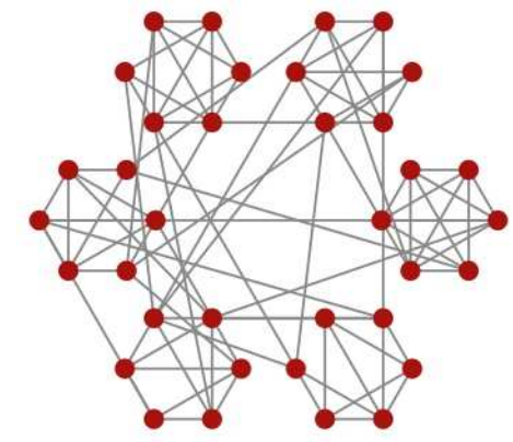
Figure 4: Relaxed caveman graph. Picture from Judd et al Judd et al. (2011).

The structure of relaxed caveman graphs is particularly useful for evaluating algorithms for chordal completions. Namely, the modifications in the edges lead to large chordless cycles, enforcing thus the inclusion of several edges in chordal completions. For our experiments, ten instances of each possible configuration involving $\alpha,\beta\in\{4,5,6,7,8\}$ and $\gamma=0.30$ were generated. This set of graphs will be henceforth denoted simply by caveman instances.

The next set of instances, grid graphs, correspond to graphs whose node set can be partitioned into a set of $r$ rows $R_{1},\dots,R_{r}$ and $c$ columns $C_{1},\dots,C_{c}$. Each vertex is denoted by $v_{r,c}$ if $v_{r,c}\in R_{r}\cap C_{c}$. Vertices $v_{i,j}$ and $v_{k,l}$ are adjacent if and only if either $i=k$ and $|j-l|=1$, or $j=l$ and $|i-k|=1$. Note that grid graphs also contain large chordless cycles.

We also used queen graphs for our experiments. The queen graphs are extensions of grid graphs with additional edges representing longer hops as well as diagonal movements. More precisely, there exists an edge connecting $v_{i,j}$ to $v_{i^{\prime},j^{\prime}}$ if and only if one of the three following conditions is satisfied for some $k$: (1) $i=i^{\prime}\pm k$ and $j=j^{\prime}\pm k$, (2) $i=i^{\prime}$ and $j=j^{\prime}\pm k$, or (3) $i=i^{\prime}\pm k$ and $j=j^{\prime}$. The configurations of grid graphs and of queen graphs used in our experiments are equivalent to those used by Yüceoğlu (2015).

The final set of instances consists of the classical DIMACS graph coloring instances, which can be downloaded from http://dimacs.rutgers.edu/Challenges/. These instances are frequently used in computational evaluations of graph algorithms.

8.2 Other Approaches

The state-of-the-art approaches to the MCCP reported in the literature are a branch-and-cut approach by Yüceoğlu (2015) and a Benders decomposition approach by Bergman and Raghunathan (2015), henceforth denoted by YUC and BEN, respectively.

YUC is based on a perfect elimination ordering (PEO) model of the MCCP. The model finds a PEO that minimizes the number of fill-in edges, and can be written as follows.

$$\min\quad \sum_{(i,j)\in{E^{c}}}y_{ij}+y_{ji}$$

s.t. $$x_{ij}+x_{ji}=1,\quad \{i,j\}\in{E}$$ for all (2)

$$x_{ij}+x_{ji}\leq 1,\quad \{i,j\}\in{E^{c}}$$ for all (3)

$$x_{ij}+x_{jk}-x_{ik}\leq 1,\quad i,j,k\in V,i\neq j,j\neq k,i\neq k$$ for all (4)

$$y_{ij}\leq x_{ij},y_{ji}\leq x_{ji},\quad i,j\in V,i\neq j$$ for all (5)

$$y_{ij}=x_{ij},y_{ji}=x_{ji},\quad \{i,j\}\in E$$ for all (6)

$$x_{jk}+y_{ij}+y_{ik}-y_{jk}\leq 2,\quad i,j,k\in V,i\neq j,j\neq k,i\neq k$$ for all (7)

$$y_{ij},x_{ij}\in\{0,1\},\quad i,j\in V,i\neq j$$ for all (8)

In the model above, denoted by PEO, a binary variable $y_{ij}$ indicates whether edge $\{i,j\}$ is added to $G$ and binary variable $x_{ij}$ indicates whether vertex $i$ precedes $j$ in the resulting ordering. Constraints (2) enforce the existence of a precedence relation between vertices $i$ and $j$ if $\{i,j\}\in E$, whereas constraints (3) prevent $i$ and $j$ from preceding each other simultaneously in an elimination ordering. Constraints (4) ensure the transitive closure of precedence relations is satisfied. Constraints (5) and (6) indicate that a precedence relation between edges $i$ and $j$ can exist if and only if $\{i,j\}\in E$. Finally, constraints (7) impose that the final ordering must be a perfect elimination ordering.

YUC employs a branch-and-cut approach that is based on a polyhedral analysis of the convex hull of solutions to PEO. Additionally, the algorithm also considers valid inequalities for special structured graphs, such as grid and queen graphs.

The other approach tested against is BEN, the precursor of the approach described in the present work. In Bergman and Raghunathan (2015), a formulation consisting only of inequalities (I1) is used in a pure Benders decomposition approach. That is, BEN solves to optimality an IP using the current set of inequalities (I1) (i.e., the Benders cuts) found up to the current iteration. If the solution contains no chordless cycles, its optimality is proven and the procedure stops. Otherwise, a collection of chordless cycles is found and new Benders cuts (i.e., inequalities (I1) violated by the current solution) are added to the model, and the procedure repeats.

Also of interest is to compare our approach with state-of-the-art heuristics in terms of solution quality, assessing thus how significant the differences between exact and heuristic solutions are. We consider the state-of-the-art heuristic developed by George and Liu (1989) (described in Section 7.3), which will be henceforth denoted by MDO.

The methodology proposed in this paper will be henceforth denoted by BC, as it can also be classified as a branch-and-cut algorithm.

8.3 Algorithmic Enhancements

In the first set of experiments, we test the following algorithmic enhancements to BC: (1) using only inequalities (I1) versus using all inequalities (I1)-(I4); (2) separating the inequalities only at integer solutions or at each search-tree node; and (3) invoking MDO as a primal heuristic. In particular, BC-Base is an implementation of BC where only inequality (I1) is considered, the separation algorithm is invoked only at integer search-tree nodes, and no primal heuristic is applied. BC-Enh is an implementation of BC where all enhancements are applied. The caveman graphs are used for this evaluation.

In order to verify whether an individual enhancement leads to a statistically significant reduction in the solution times, a two-sample paired t-test was employed. Specifically, the null hypothesis indicates whether the solutions times are equivalent with or without the enhancements. Solution times can differ by orders of magnitude across the 250 instances of caveman graphs (e.g., 0.001 seconds versus nearly 3,600 seconds), so all comparisons were made in logarithmic scale, i.e., we applied $\log(1+t)$ transformations to run times $t$ (given in seconds).

For enhancement (1), (2), and (3) taken individually, the tests resulted in a p-value of 0.070, 0.00057, and 0.0013, respectively. This shows that each enhancement provides considerable reductions in run time, with the heuristic being perhaps the most effective among them. When comparing BC-Base versus BC-Enh, the test yields a p-value 0.0000067, showing strong statistical significance of the results indicating reductions on run times caused by the enhancements.

A plot comparing the solution times of BC-Base and BC-Enh is provided in Figure 5. Each point in the scatter plot of Figure 5(a) corresponds to one instance, with the radii indicating the sizes of the cliques and the color representing the number of cliques (dark red/blue corresponding to instances with smallest/largest number of cliques, respectively). The $x$-axis is the run time in seconds in log-scale for BC-Base and the $y$-axis contains the respective values for BC-Enh. Figure 5(b) presents the cumulative distribution plot of performance of both algorithms, indicating in the $y$-axis how many instances were solved within the amount of time indicated in the $x$-axis. Both figures shows that BC-Enh typically outperforms BC-Base, which becomes more prominent with harder instances.

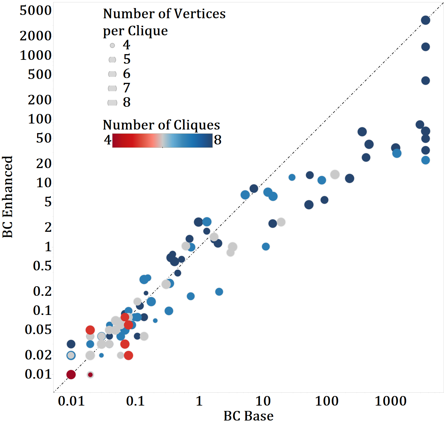
(a) Scatter plot

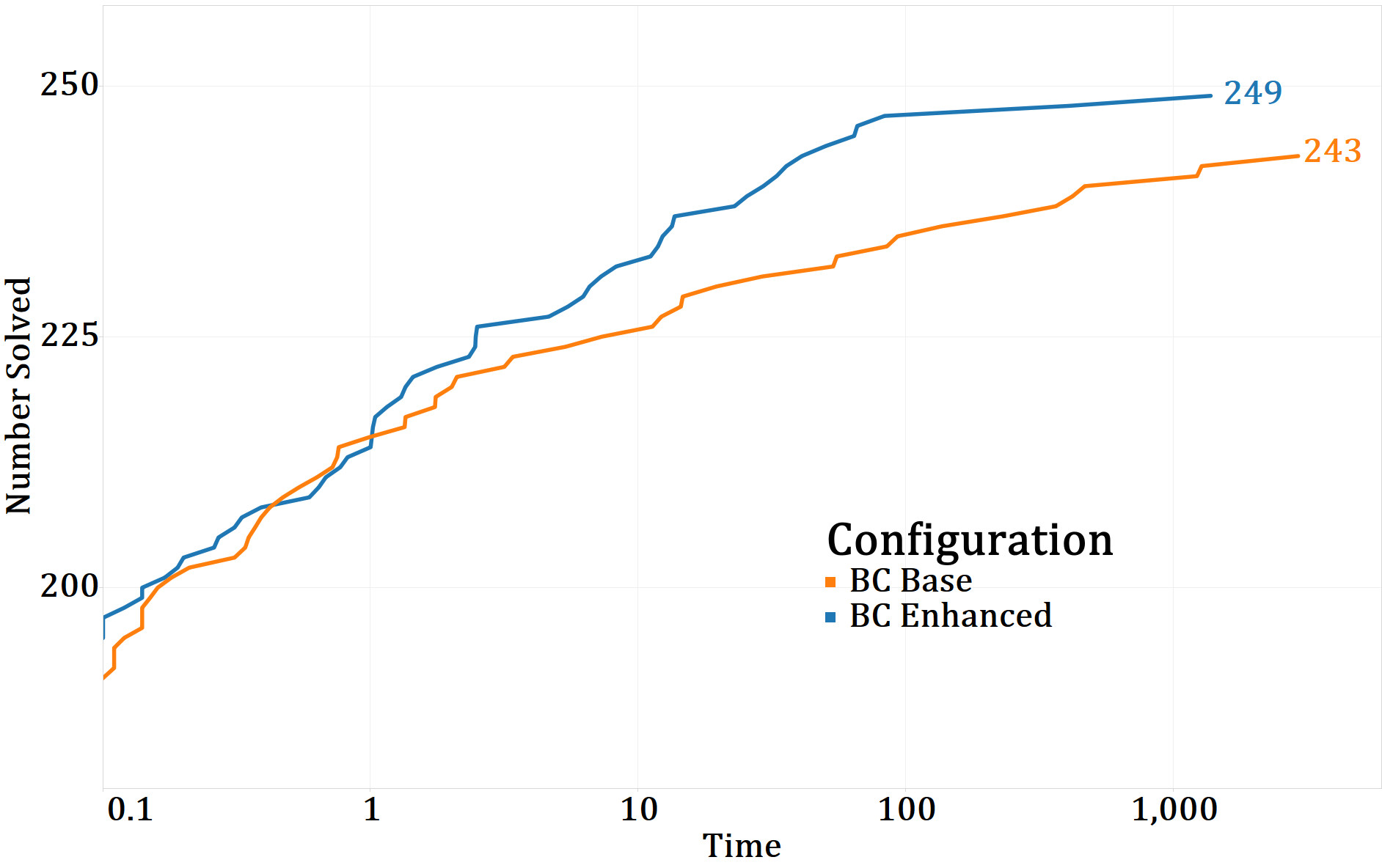
(b) Cumulative distribution plots of performance

Figure 5: Comparing BC with and without algorithmic enhancements on caveman graphs. (a) Scatter plot comparing solution times, with the size of the dot corresponding to the number of vertices in each clique and the color (red to blue) the relative number of cliques. (b) Cumulative distribution plot of performance showing number of instances solved by a certain time limit.

The algorithmic enhancements provide clear computational advantages, and so we use them for the remaining experiments, referring to BC-Enh simply as BC.

8.4 Comparison with Heuristics

In the second set of experiments, we investigate the improvements brought by BC upon the solutions obtained alone by MDO. Note that, since BC uses MDO at the root and throughout search, the solutions will always be at least as good as those achieved by MDO.

Our first comparison, involving the relaxed caveman graphs, is presented in Table 1. For each configuration, the averages of the upper bounds provided by both BC and MDO are presented, as well as the average percentage decreases in the upper bound from MDO to BC and the average times to compute the chordal completion. As MDO achieves solutions in under a hundredth of a second in all cases, its running times are not reported. These results readily show the advantage of seeking optimal solutions. The heuristic can be far from the optimal solution (eventually by up to 70%) and, on the relaxed caveman graphs, the running time of BC is almost always small (only one instance is not proven optimal within 3,600 seconds).

Table 1: Comparison between MDO and BC on caveman graphs.

$\alpha$	$\beta$	BC UB	MDO UB	% Dec	BC Time
4	4	0.9	1.4	15	0
4	5	1.7	2.8	35.1	0
4	6	5.3	7.4	42.8	0
4	7	13.2	17.3	25.1	0
4	8	19	26.3	29.3	0
5	4	1.6	1.8	6.3	0
5	5	1.7	4.4	51.8	0
5	6	7.7	10.3	40.3	0
5	7	15.5	21.7	35.7	1.3
5	8	25.1	37.1	34.8	0.5
6	4	0.6	1.7	32.1	0
6	5	4.1	8.4	54.9	0
6	6	12.2	16.9	35.4	0.1
6	7	18.1	24.2	25.3	0.1
6	8	28.9	43	35.8	2.0
7	4	1.1	2.5	50.8	0
7	5	3.6	6.5	42.9	0
7	6	17.1	23.6	35.8	0.5
7	7	24.8	35.4	37.6	3.5
7	8	55.9	74.1	27.6	198.9
8	4	0.3	3.3	70.8	0
8	5	5.5	9.9	58.7	0
8	6	14.6	23.3	39.9	1.5
8	7	29.7	45	37.6	5.2
8	8	52.4	69.8	26.2	382.2

The same data for grid graphs, queen graphs, and DIMACS graphs are presented in Tables 2, 3, and 4, respectively. These tables first report the graph characteristics, including number of vertices and number of edges, and for all algorithms the resulting lower bounds, upper bounds, and solution times (in seconds if solved to optimality in 3,600s, or a mark ”-” otherwise), respectively. Bold face for the upper bound indicates that the algorithm found the best-known solution for the instance. In general, BC can deliver better solutions than MDO but requires much more time in harder instances, showing therefore the trade-off in computational time and solution quality.

8.5 Comparison with Other Techniques

This section provides a comparison of BC with YUC and BEN. For these evaluations, we employed all instances reported upon in Yüceoğlu (2015) and Bergman and Raghunathan (2015) and compared the solution times and objective function bounds obtained by all solution methods. The reported numbers for YUC were obtained directly from Yüceoğlu (2015), who uses IBM ILOG CPLEX 12.2 and a processor with similar clock (2.53 GHz), but runs the parallel version of the solver with 4 cores, and not with 1 core, as we do in this work.

First, we report on grid graphs, which were used in the computational results of Yüceoğlu (2015) for YUC. This approach enhances the PEO formulation with cuts tailored for graphs containing grid structures, so these instances are particularly well-suited for YUC. The results are presented in Table 2. BC typically finds the best-known solutions, and only in 4 cases out of 22 the relaxation bound for YUC outperforms that of BC.

Table 2: Results for grid graphs. Note: Graph grid5_5 was not included in the results reported on in Yüceoğlu (2015).

	Instance				YUC				BC			MDO
name	$|V|$	$|E|$		$LB$	$UB$	$t$		$LB$	$UB$	$t$		$UB$
grid3_3	9	12		5	5	0.01		5	5	0		5
grid3_4	12	17		9	9	0		9	9	0.01		9
grid3_5	15	22		13	13	0.02		13	13	0.07		13
grid3_6	18	27		17	17	0.02		17	17	0.17		17
grid3_7	21	32		21	21	0.01		21	21	0.22		21
grid3_8	24	37		25	25	0.02		25	25	1.39		25
grid3_9	27	42		29	29	0.02		29	29	9.13		33
grid3_10	30	47		33	33	0.03		33	33	20.39		37
grid4_4	16	24		18	18	1.23		18	18	2.33		18
grid4_5	20	31		25	25	18.11		25	25	8.35		25
grid4_6	24	38		32.2	34	-		34	34	216.71		34
grid4_7	28	45		39	41	-		41	41	304.85		41
grid4_8	32	52		45.5	52	-		48.2	50	-		50
grid4_9	36	59		52.5	58	-		54.2	57	-		57
grid4_10	40	66		59.3	66	-		59.1	66	-		66
grid5_5	25	40		*	*	*		37	37	115.98		37
grid5_6	30	49		46.2	53	-		48.7	50	-		52
grid5_7	35	58		56.9	65	-		56.5	62	-		68
grid5_8	40	67		67.5	77	-		65.2	75	-		80
grid5_9	45	76		33.3	90	-		73.2	89	-		93
grid6_6	36	60		60.9	77	-		59.2	69	-		71
grid6_7	42	71		31	94	-		69.1	88	-		92
grid7_7	49	84		37	125	-		80.3	112	-		119

Table 3: Results for queen graphs.

	Instance				YUC				BC			MDO
name	$|V|$	$|E|$		$LB$	$UB$	$t$		$LB$	$UB$	$t$		$UB$
queen3_3	9	28		5	5	0		5	5	0		5
queen3_4	12	46		12	12	0.01		12	12	0.01		12
queen3_5	15	67		22	22	0.31		22	22	0.03		22
queen3_6	18	91		36	36	1.03		36	36	0.25		36
queen3_7	21	118		53	53	2.17		53	53	0.91		53
queen3_8	24	148		74	74	8.49		74	74	2.27		74
queen3_9	27	181		98	98	15.77		98	98	4.97		98
queen3_10	30	217		126	126	65.91		126	126	22.29		126
queen4_4	16	76		26	26	0.19		26	26	0.03		28
queen4_5	20	110		51	51	4.54		51	51	0.75		53
queen4_6	24	148		83	83	16.54		83	83	6.68		83
queen4_7	28	190		119	119	68.22		119	119	34.5		121
queen4_8	32	236		164	164	636.28		164	164	445.78		167
queen4_9	36	286		209.8	217	-		211.4	217	-		222
queen4_10	40	340		255.5	278	-		259.7	278	-		286
queen5_5	25	160		93	93	41.03		93	93	14.02		94
queen5_6	30	215		144	144	185.81		144	144	186.93		154
queen5_7	35	275		203.1	214	-		204.2	214	-		223
queen5_8	40	340		265.8	293	-		265.5	293	-		306
queen5_9	45	410		339.8	393	-		338.8	386	-		398
queen5_10	50	485		424.9	501	-		424	492	-		503
queen6_6	36	290		214.9	232	-		218.1	231	-		244
queen6_7	42	371		299.2	351	-		296.4	338	-		352
queen6_8	48	458		400.7	481	-		396.5	461	-		482
queen6_9	54	551		521.4	622	-		514.3	619	-		633
queen6_10	60	650		656.7	786	-		646.6	787	-		826
queen7_7	49	476		423.7	520	-		422.3	495	-		515
queen7_8	56	588		577.6	710	-		567.2	680	-		687
queen7_9	63	707		751.8	935	-		736.8	897	-		919
queen7_10	70	833		948.5	1177	-		926.6	1141	-		1149
queen8_8	64	728		782.1	965	-		766.9	939	-		970

Next, Table 3 reports on queen graphs. As previously mentioned, these instances are also well-suited to YUC because of their grid-like structures. Nonetheless, the results show that BC typically outperforms YUC both in terms of optimality gap and solution time. In particular, for almost all instances, the obtained solution is at least as good as the one found by YUC. In the only exception, the solution obtained by BC contains only one fill edge more than YUC.

Finally, Table 4 reports on DIMACS graphs. The 12 instances above the double horizontal line are those reported on in Yüceoğlu (2015), whereas the others are the remaining graphs in the benchmark set with fewer than 150 vertices. Our results show that instances of the first group are solved orders of magnitude faster by BC and, for those in which YUC was not able to prove optimality, better objective function bounds are obtained. In particular, BC was able to close entirely the optimality gap of four instances of this dataset that were still open: david, miles250, miles750, and myciel5. These results can be explained by the fact that DIMACS graphs do not necessarily have grid-like structures, which makes them more challenging for YUC. For the remaining instances, 9 are solved to optimality and for many of the other instances, the best solutions obtained by BC employed substantially fewer fill edges than those obtained by the traditional heuristic MDO.

Table 4: Results for dimacs graphs.

	Instance				YUC				BC			MDO
name	$|V|$	$|E|$		$LB$	$UB$	$t$		$LB$	$UB$	$t$		$UB$
anna	138	493		47	47	1386.04		47	47	1.02		47
david	87	406		59.5	65	-		64	64	0.4		66
games120	120	638		496.4	1626	-		886.7	1503	-		1513
huck	74	301		5	5	2.92		5	5	0.04		9
jean	80	254		16	16	6.13		16	16	0.09		19
miles250	128	387		45.7	61	-		53	53	0.4		61
miles500	128	1170		196.4	447	-		327.487	376	-		446
miles750	128	2113		352.1	954	-		471	471	537.65		723
myciel3	11	20		10	10	0		10	10	0		10
myciel4	23	71		46	46	0.06		46	46	0.03		46
myciel5	47	236		189.7	197	-		196	196	28.93		197
1-FullIns_3	30	100						80	80	2.42		80
1-FullIns_4	93	593						657.9	785	-		839
1-Insertions_4	67	232						303.6	365	-		394
2-FullIns_3	52	201						230.4	248	-		273
2-Insertions_3	37	72						85.1	99	-		103
2-Insertions_4	149	541						659.3	1585	-		1588
3-FullIns_3	80	346						407.1	577	-		661
3-Insertions_3	56	110						118.4	192	-		198
4-FullIns_3	114	541						691.8	1094	-		1274
4-Insertions_3	79	156						155.8	330	-		331
DSJC125.1	125	736						1752.3	2618	-		2618
DSJC125.5	125	3891						2381.7	3240	-		3240
DSJC125.9	125	6961						600.6	734	-		734
miles1000	128	3216						535	535	331.2		700
miles1500	128	5198						218	218	1.65		308
mug100_1	100	166						64	64	0.3		91
mug100_25	100	166						64	64	0.51		93
mug88_1	88	146						56	56	0.22		82
mug88_25	88	146						56	56	0.49		84
myciel6	95	755						741.3	753	-		753
r125.1	125	209						11	11	0.17		15
r125.1c	125	7501						207	207	26.83		207
r125.5	125	3838						895.4	1231	-		1231

We conclude this section by comparing our results with those presented in Bergman and Raghunathan (2015). With the exception of some queen instances, BC always provides better solutions and objective bounds than BEN. In the exceptional cases, the bounds provided by BEN were slightly better. Note also that BEN does not provide any feasible solution until the algorithm terminates.

8.6 Cuts Found

This section provides an analysis of the types of cuts found by BC during the solution process across all experiments. Figure 6 (a) shows an area plot depicting the distribution of the number of inequalities of each type that was identified and added to the model in BC. We present only the 88 instances for which at least 10,000 cuts were added, where all graph classes were considered, and the instances are ordered by total number of cuts found. This plot readily shows that most of the cuts added were of type (I2) and (I4).

Figure 6 (b) shows an area plot depicting a similar comparison, but between those cuts added at integer nodes and those added by the threshold separation procedure from §7. For the majority of instances, the cuts are predominantely found through threshold cuts. The far right portion of the plot corresponds to relatively large instances, hence only a few branching nodes were explored.

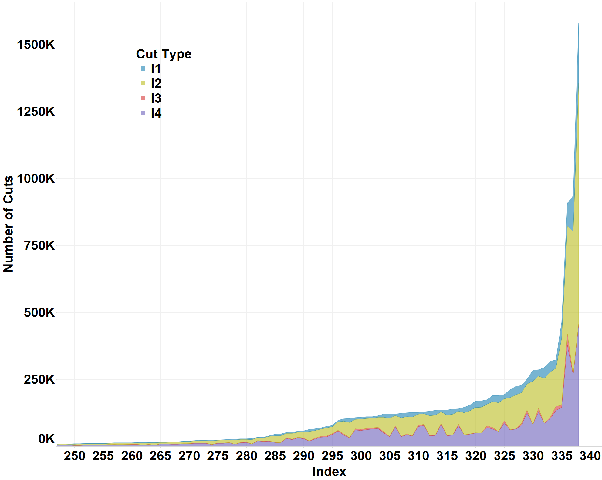
(a) Comparing counts of inequalities

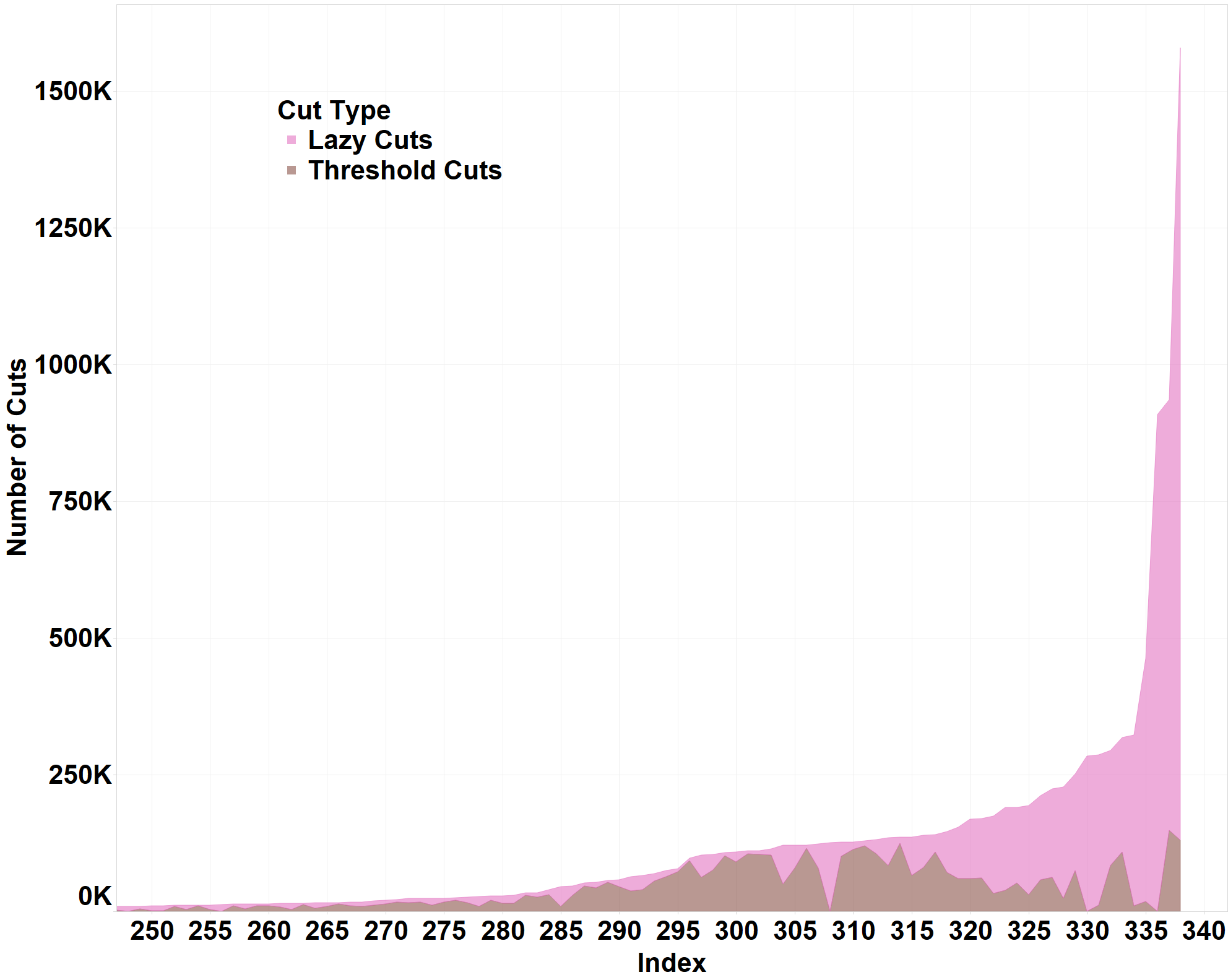
(b) Comparing mode of cut identification

Figure 6: Area plots displaying types of cuts found and added by BC across all instances.

9 Conclusion

In this paper we described a new mathematical programming formulation for the MCCP and investigated some key properties of its polytope. The constraints employed in our model correspond to lifted inequalities of induced cycle graphs, and our theoretical results show that this lifting procedure can be generalized to derive other facets of the MCCP polytope of cycle graphs. Finally, we proposed a hybrid solution technique that considers both a lazy-constraint generation and a heuristic separation method based on a threshold rounding, and also presented a simple primal heuristic for the problem. A numerical study indicates that our approach substantially outperforms existing methods, often by orders of magnitude, and, in particular, solves many benchmark graphs to optimality for the first time.

Online Supplement - Proofs of Statements

10 Additional Proofs for Section 5

Proof 10.1

Facet-defining proof of Proposition 5.1. Let $F^{I}=\left\{x\in X(G):\sum_{f\>\in\>\textnormal{int}(C)}x_{f}=|C|-3\right\}$ and $\mu x\geq\mu_{0}$ be a valid inequality for $\mathrm{conv}(X(G))$ which is satisfied at equality by each $x\in F^{I}$. It suffices to show that there exists some $\lambda$ for which $\mu_{f}=\lambda$ and $\mu_{0}=(|C|-3)\lambda$.

Let $x^{\prime}\in\{0,1\}^{m^{c}}$ be defined by

$$x^{\prime}_{f}=\left\{\begin{array}[]{ll}1,&\quad f=\{v_{0},v_{j}\},j=2,\ldots,k-2;\\ 0,&\quad\mbox{otherwise}.\end{array}\right.$$

Claim 1

$x^{\prime}\in X(G)$, i.e., $G(x^{\prime})$ is chordal, and $x^{\prime}\in F^{I}$.

References

- Beeri et al. (1983) Beeri C, Fagin R, Maier D, Yannakakis M (1983) On the desirability of acyclic database schemes. J. ACM 30(3):479–513, ISSN 0004-5411, URL http://dx.doi.org/10.1145/2402.322389.
- Bergman and Cire (2016) Bergman D, Cire A (2016) Decompositions based on decision diagrams. CPAIOR 2016, to appear .
- Bergman and Raghunathan (2015) Bergman D, Raghunathan AU (2015) A benders approach to the minimum chordal completion problem. Principles and Practice of Constraint Programming – CP 2015, volume 6308 of Lecture Notes in Computer Science, 47–64 (Springer Berlin Heidelberg).
- Berry et al. (2006) Berry A, Bordat JP, Heggernes P, Simonet G, Villanger Y (2006) A wide-range algorithm for minimal triangulation from an arbitrary ordering. Journal of Algorithms 58(1):33 – 66, ISSN 0196-6774, URL http://dx.doi.org/http://dx.doi.org/10.1016/j.jalgor.2004.07.001.
- Berry et al. (2003) Berry A, Heggernes P, Simonet G (2003) The minimum degree heuristic and the minimal triangulation process. Bodlaender H, ed., Graph-Theoretic Concepts in Computer Science, volume 2880 of Lecture Notes in Computer Science, 58–70 (Springer Berlin Heidelberg), ISBN 978-3-540-20452-7, URL http://dx.doi.org/10.1007/978-3-540-39890-5_6.
- Bodlaender et al. (1998) Bodlaender HL, Kloks T, Kratsch D, Mueller H (1998) Treewidth and minimum fill-in on d-trapezoid graphs.
- Broersma et al. (1997) Broersma H, Dahlhaus E, Kloks T (1997) Algorithms for the treewidth and minimum fill-in of HHD-free graphs. Möhring R, ed., Graph-Theoretic Concepts in Computer Science, volume 1335 of Lecture Notes in Computer Science, 109–117 (Springer Berlin Heidelberg), ISBN 978-3-540-63757-8, URL http://dx.doi.org/10.1007/BFb0024492.
- Chang (1996) Chang MS (1996) Algorithms for maximum matching and minimum fill-in on chordal bipartite graphs. Asano T, Igarashi Y, Nagamochi H, Miyano S, Suri S, eds., Algorithms and Computation, volume 1178 of Lecture Notes in Computer Science, 146–155 (Springer Berlin Heidelberg), ISBN 978-3-540-62048-8, URL http://dx.doi.org/10.1007/BFb0009490.
- Chung and Mumford (1994) Chung F, Mumford D (1994) Chordal completions of planar graphs. Journal of Combinatorial Theory, Series B 62(1):96 – 106, ISSN 0095-8956, URL http://dx.doi.org/http://dx.doi.org/10.1006/jctb.1994.1056.
- Codato and Fischetti (2006) Codato G, Fischetti M (2006) Combinatorial benders’ cuts for mixed-integer linear programming. Operations Research 54(4):756–766, URL http://dx.doi.org/10.1287/opre.1060.0286.
- Cormen et al. (2009) Cormen TH, Leiserson CE, Rivest RL, Stein C (2009) Introduction to Algorithms, Third Edition (The MIT Press), 3rd edition, ISBN 0262033844, 9780262033848.
- Feremans et al. (2002) Feremans C, Oswald M, Reinelt G (2002) A y-formulation for the treewidth. Technical report, Heidelberg University.
- Fomin et al. (2013) Fomin FV, Philip G, Villanger Y (2013) Minimum fill-in of sparse graphs: Kernelization and approximation. Algorithmica 71(1):1–20, ISSN 1432-0541, URL http://dx.doi.org/10.1007/s00453-013-9776-1.
- Fomin and Villanger (2012) Fomin FV, Villanger Y (2012) Subexponential parameterized algorithm for minimum fill-in. Proceedings of the Twenty-third Annual ACM-SIAM Symposium on Discrete Algorithms, 1737–1746, SODA ’12 (SIAM), URL http://dl.acm.org/citation.cfm?id=2095116.2095254.
- Fulkerson and Gross (1965) Fulkerson DR, Gross OA (1965) Incidence matrices and interval graphs. Pacific J. Math. 15(3):835–855, URL http://projecteuclid.org/euclid.pjm/1102995572.
- Garey and Johnson (1979) Garey MR, Johnson DS (1979) Computers and Intractability: A Guide to the Theory of NP-Completeness (New York, NY, USA: W. H. Freeman & Co.), ISBN 0716710447.
- George and Liu (1989) George A, Liu WH (1989) The evolution of the minimum degree ordering algorithm. SIAM Rev. 31(1):1–19, ISSN 0036-1445, URL http://dx.doi.org/10.1137/1031001.
- Grone et al. (1984) Grone R, Johnson CR, Sá EM, Wolkowicz H (1984) Positive definite completions of partial hermitian matrices. Linear Algebra and its Applications 58(0):109 – 124, ISSN 0024-3795, URL http://dx.doi.org/http://dx.doi.org/10.1016/0024-3795(84)90207-6.
- Heggernes (2006) Heggernes P (2006) Minimal triangulations of graphs: A survey. Discrete Mathematics 306(3):297 – 317, ISSN 0012-365X, URL http://dx.doi.org/http://dx.doi.org/10.1016/j.disc.2005.12.003, minimal Separation and Minimal Triangulation.
- IBM ILOG (2016) IBM ILOG (2016) Cplex optimization studio 12.6.3 user manual.
- Judd et al. (2011) Judd S, Kearns M, Vorobeychik Y (2011) Behavioral conflict and fairness in social networks. Chen N, Elkind E, Koutsoupias E, eds., Internet and Network Economics, volume 7090 of Lecture Notes in Computer Science, 242–253 (Springer Berlin Heidelberg), ISBN 978-3-642-25509-0, URL http://dx.doi.org/10.1007/978-3-642-25510-6_21.
- Kaplan et al. (1999) Kaplan H, Shamir R, Tarjan RE (1999) Tractability of parameterized completion problems on chordal, strongly chordal, and proper interval graphs. SIAM Journal on Computing 28(5):1906–1922, URL http://dx.doi.org/10.1137/S0097539796303044.
- Kim et al. (2011) Kim S, Kojima M, Mevissen M, Yamashita M (2011) Exploiting sparsity in linear and nonlinear matrix inequalities via positive semidefinite matrix completion. Mathematical Programming 129(1):33–68, ISSN 0025-5610, URL http://dx.doi.org/10.1007/s10107-010-0402-6.
- Kloks et al. (1998) Kloks T, Kratsch D, Wong C (1998) Minimum fill-in on circle and circular-arc graphs. Journal of Algorithms 28(2):272 – 289, ISSN 0196-6774, URL http://dx.doi.org/http://dx.doi.org/10.1006/jagm.1998.0936.
- Lauritzen and Spiegelhalter (1990) Lauritzen SL, Spiegelhalter DJ (1990) Local computations with probabilities on graphical structures and their application to expert systems. Shafer G, Pearl J, eds., Readings in Uncertain Reasoning, 415–448 (San Francisco, CA, USA: Morgan Kaufmann Publishers Inc.), ISBN 1-55860-125-2, URL http://dl.acm.org/citation.cfm?id=84628.85343.
- Mezzini and Moscarini (2010) Mezzini M, Moscarini M (2010) Simple algorithms for minimal triangulation of a graph and backward selection of a decomposable Markov network. Theoretical Computer Science 411(7–9):958 – 966, ISSN 0304-3975, URL http://dx.doi.org/http://dx.doi.org/10.1016/j.tcs.2009.10.004.
- Nakata et al. (2003) Nakata K, Fujisawa K, Fukuda M, Kojima M, Murota K (2003) Exploiting sparsity in semidefinite programming via matrix completion II: implementation and numerical results. Mathematical Programming 95(2):303–327, ISSN 0025-5610, URL http://dx.doi.org/10.1007/s10107-002-0351-9.
- Rollon and Larrosa (2011) Rollon E, Larrosa J (2011) Principles and Practice of Constraint Programming – CP 2011: 17th International Conference, CP 2011, Perugia, Italy, September 12-16, 2011. Proceedings, chapter On Mini-Buckets and the Min-fill Elimination Ordering, 759–773 (Berlin, Heidelberg: Springer Berlin Heidelberg), ISBN 978-3-642-23786-7, URL http://dx.doi.org/10.1007/978-3-642-23786-7_57.
- Rose and Tarjan (1978) Rose DJ, Tarjan RE (1978) Algorithmic aspects of vertex elimination on directed graphs. SIAM Journal on Applied Mathematics 34(1):176–197, URL http://dx.doi.org/10.1137/0134014.
- Rose et al. (1976) Rose DJ, Tarjan RE, Lueker GS (1976) Algorithmic aspects of vertex elimination on graphs. SIAM Journal on Computing 5(2):266–283, URL http://dx.doi.org/10.1137/0205021.
- Rostami et al. (2015) Rostami B, Malucelli F, Frey D, Buchheim C (2015) On the quadratic shortest path problem. International Symposium on Experimental Algorithms, 379–390 (Springer).
- Tarjan and Yannakakis (1984) Tarjan RE, Yannakakis M (1984) Simple linear-time algorithms to test chordality of graphs, test acyclicity of hypergraphs, and selectively reduce acyclic hypergraphs. SIAM J. Comput. 13(3):566–579, ISSN 0097-5397, URL http://dx.doi.org/10.1137/0213035.
- Vandenberghe and Andersen (2015) Vandenberghe L, Andersen MS (2015) Chordal graphs and semidefinite optimization. Foundations and Trends in Optimization 1(4):241–433, ISSN 2167-3888, URL http://dx.doi.org/10.1561/2400000006.
- Yannakakis (1981) Yannakakis M (1981) Computing the minimum fill-in is NP-Complete. SIAM Journal on Algebraic Discrete Methods 2(1):77–79, URL http://dx.doi.org/10.1137/0602010.
- Yüceoğlu (2015) Yüceoğlu B (2015) Branch-and-cut algorithms for graph problems. Ph.D. thesis, Maastricht University, URL http://digitalarchive.maastrichtuniversity.nl/fedora/get/guid:bde57abf-9652-45bc-8590-667e7e085074/ASSET1.