Dynamic Network Reconstruction from
Heterogeneous Datasets
(Supplementary Version)

Abstract

Performing multiple experiments is common when learning internal mechanisms of complex systems. These experiments can include perturbations to parameters or external disturbances. A challenging problem is to efficiently incorporate all collected data simultaneously to infer the underlying dynamic network. This paper addresses the reconstruction of dynamic networks from heterogeneous datasets under the assumption that underlying networks share the same Boolean structure across all experiments. Parametric models for dynamical structure functions are derived to describe causal interactions between measured variables. Multiple datasets are integrated into one regression problem with additional demands of group sparsity to assure network sparsity and structure consistency. To acquire structured group sparsity, we propose a sampling-based method, together with extended versions of $l_{1}$ methods and sparse Bayesian learning. The performance of the proposed methods is benchmarked in numerical simulation. In summary, this paper presents efficient methods on network reconstruction from multiple experiments, and reveals practical experience that could guide applications.

, , , ,

1 Introduction

Network reconstruction has been widely applied in different fields to learn interaction structures or dynamic behaviours, including systems biology, computer vision, econometrics, social networks, etc. With increasingly easy access to time-series data, it is expected that networks can help to explain dynamics, causal interactions and internal mechanisms of complex systems. For instance, biologists use causal network inference to determine critical genes that are responsible for diseases in pathology, e.g. [1].

Boolean networks are introduced in [2, 3] to approximate the dynamics of an underlying processes by Markov chain models with binary state-transition matrices. However, it may fail to capture complex dynamics. Another popular model is Bayesian networks, e.g. [4]. Although it delivers causality information, Bayesian networks are defined as a type of directed acyclic graphs (see [5, p. 127] for domains of probabilistic models). Feedback loops are particularly important in applications. Even though dynamic Bayesian network is able to handle loops in digraphs [6], it requires huge amounts of data (repetitive measurements of each time point), which may not be practical in biology. Regarding causality, Granger causality (GC) is originally proposed in [7] and defined in general based on conditional independence (see e.g. [8]). However, as mentioned in [7], this approach may be “problematic in deterministic settings, especially in dynamic systems with weak to moderate coupling” [9]. With minor conditions on spectral density, GC can be inferred by estimating vector autoregression models [10]. A recent work [11] proposes a kernel-based system identification method with sparsity constraints to infer GC graphs.

There have been many applications of network reconstruction by identifying simplified dynamical models, e.g. [12], [13] and [14]. However, identifiability remains untouched in these study, which is essential to guarantee reliability of results. To study network identifiability, the work in [15] proposed dynamical structure functions (DSFs) for linear time-invariant (LTI) systems as a general network representation. Similar network models appeared in [16, 17], and their differences are discussed in [18]. Theoretical results on network identifiability were firstly presented in [15]. Successive work in [19, 20] studies network identifiability from intrinsic noise and [21] presents identifiability results for sparse networks. Moreover, there is a structural point of view for topological identification of networks from data, e.g., [22, 23].

Many biological applications have replica to remove effects of noise. However, only a handful of or less replica are typically available in practice, meaning that averages may not be statistically significant. The work in [24] proposes an idea to integrate replica data as a whole, which will be adopted in this paper. It considers a particular reconstruction problem for nonlinear systems, which assumes full-state measurements (no hidden states), basis functions known a priori and linearity in parameters. Our work will focus on general network reconstruction problems of LTI systems, with existence of hidden states. In practice, system parameters in multiple experiments can be fairly different due to high variability of biological processes [25]. On the other hand, for identical organisms, the interconnection structure, e.g. genetic regulation, should be identical over experimental repetitions. Using DSFs as a general network model class, the method proposed in the paper allows system parameters to be fairly different, while keeping the network topology consistent across replica.

The paper is organised in modules, illustrated by Fig. 1: 1) derivation of regression problems for network reconstruction (Section 3); 2) dealing with heterogeneity data (Section 4); 3) solvers to the target optimisation problem (Section 5). The paper is closed by benchmark studies on random sparse network reconstruction. A supplement to technical details and other illustrative examples are provided as appendices in [26]. Codes in MATLAB and benchmark data are available at https://github.com/oracleyue/{dynet_dt-mat,datasets}.

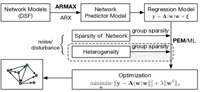
Figure 1: An overview of the network reconstruction method.

2 Problem Description

Let $Y\triangleq\{y(t),t\in\mathbb{Z}\}$, $U\triangleq\{u(t),t\in\mathbb{Z}\}$ be multivariate time series of dimension $p$ and $m$, respectively, where the elements could be deterministic ($y(t)\in\mathbb{R}^{p}$, $u(t)\in\mathbb{R}^{m}$) or be real-valued random vectors defined on probability spaces $(\Omega,\mathscr{F},\mathbb{P})$. We usually assume that $u(t)$ is deterministic in practice, which is interpreted as controlled input signals.

2.1 Linear dynamic networks

Consider the network model for LTI systems, called dynamical structure function (DSF) [15, 27],

$$y(t)=Q(q)y(t)+P(q)u(t)+H(q)e(t),$$ (1)

where $y(t)=[y_{1}(t),\dots,y_{p}(t)]^{T}$, $u(t)=[u_{1}(t),\dots,u_{m}(t)]^{T}$, a $p$-variate i.i.d. $e(t)=[e_{1}(t),\dots,e_{p}(t)]^{T}$ with zero mean and identity covariance matrix,

$$Q(q) =[Q_{ij}(q)]_{p\times p},\quad\quad Q_{ii}(q)=0,\ \forall i,$$

$$P(q) =[P_{ij}(q)]_{p\times m},\quad\quad H(q)=[H_{ij}(q)]_{p\times p}$$

$Q_{ij}(q),P_{ij}(q),H_{ij}(q)$ are single-input-single-output (SISO) real-rational transfer functions, and $q$ is the forward-shift operator, i.e. $qy(t)=y(t+1)$, $q^{-1}y(t)=y(t-1)$. Here $Q_{ij}(q)$ ($i\neq j$) are strictly proper, and $P_{ij},H_{ii}(q)$ are proper. See Appendix A in [26] for more on DSFs. The networks represented by DSFs can be defined by extending the capacity functions of standard networks in the graph theory. Let $\mathcal{G}=(V,E)$ be a digraph, where the vertex set $V=\{y_{1},\dots,y_{p},u_{1},\dots,u_{m},e_{1},\dots,e_{p}\}$, and the directed edge set $E$ is defined by

$$\begin{array}[]{@{}ll@{\;}l@{\;\,}l@{\;\,}l@{\;}l}\text{ $\centerdot$}&(y_{j},y_{i})&\in E&\Leftrightarrow&Q_{ij}(q)&\neq 0,\\ \text{ $\centerdot$}&(u_{k},y_{i})&\in E&\Leftrightarrow&P_{ik}(q)&\neq 0,\\ \text{ $\centerdot$}&(e_{l},y_{i})&\in E&\Leftrightarrow&H_{il}(q)&\neq 0,\\ \text{ $\centerdot$}&(y_{i},u_{k})&\notin E,&\,\lx@intercol(y_{i},e_{l})\notin E,\hfil\lx@intercol\end{array}$$

for all $i,j,k$ and $l$. And let the capacity function $f$ be a map defined as

$$\begin{array}[]{rr@{\;\,}c@{\;\,}l}f:&E&\rightarrow&{S}_{\text{TF}}\\ &(y_{j},y_{i})&\mapsto&Q_{ij}(q)\;\;\text{or}\;\;(u_{k},y_{i})\mapsto P_{ik}(q)\;\;\text{or}\\ &(e_{l},y_{i})&\mapsto&H_{il}(q),\end{array}$$

where ${S}_{\text{TF}}$ is a subset of single-input-single-output (SISO) proper rational transfer functions. We call the tuple $\mathcal{N}\coloneqq(\mathcal{G},f)$ a (linear) dynamic network, and $\mathcal{G}$ the underlying digraph of $\mathcal{N}$, which is also called (linear) Boolean dynamic network.

To guarantee network identifiability, i.e. unique determination of DSFs from input-output transfer functions, we need to assume either $H(q)$ or $P(q)$ being square and diagonal, e.g. see [15, 28]. Here we take the diagonal $H$ as an example, and we further assume all assumptions in [28] are satisfied.

Assumption 1.

The matrix $H$ is square, diagonal and full rank.

Alternatively, we could use general $H$ but restrict $P$ to be square and diagonal, and the forthcoming method can be easily modified correspondingly. A square and diagonal $P$ presents a practical way in experiments to guarantee network identifiability, i.e. perturbing each measured variable. Indeed, the DSF with square diagonal $H$ is fairly special, which can be equivalently rewritten such that reconstruction can be treated as identification of input-output transfer functions with sparse input selection. However, this paper uses a flexible framework that is valid for diagonal $P$ or $H$, or even other network identifiability conditions.

2.2 Network reconstruction from multiple experiments

Consider multiple experiments, where $\{Y^{[l]},U^{[l]}\}_{l=1,\dots,L}$ denote measurements from $L$ experiments. Let $\mathcal{N}((Q,P,H))$ be the dynamic network $\mathcal{N}$ determined by $(Q,P,H)$, and $\mathcal{G}((Q,P,H))$ be the corresponding Boolean dynamic network. The governing model (1) could be different in each experiment, denoted by $(Q,P,H)^{[l]},l=1,\dots,L$. In addition, $\mathcal{N}^{0}$ denotes a fixed dynamic network, and $\mathcal{G}^{0}$ a fixed Boolean dynamic network. The datasets $\{Y^{[l]},U^{[l]}\}_{l=1,\dots,L}$ are called homogeneous, if $\mathcal{N}((Q,P,H)^{[l]})\equiv\mathcal{N}^{0},\forall l$, i.e. the measurements in multiple experiments are from the same dynamic network. And the datasets $\{Y^{[l]},U^{[l]}\}_{l=1,\dots,L}$ are said to be heterogeneous, if $\mathcal{G}((Q,P,H)^{[l]})\equiv\mathcal{G}_{0},\forall l$ but $\mathcal{N}((Q,P,H)^{[l]})$ are different between certain $l\in\{1,\dots,L\}$. The constraint $\mathcal{G}((Q,P,H)^{[l]})\equiv\mathcal{G}_{0}$ presents the common feature shared by systems in multiple experiments. For example, even though biological individuals are different in nature, if they are all healthy or subject to the same gene-level operations, it is fair to assume they have the same genetic regularisation.

Assumption 2.

The underlying systems in multiple experiments, which provide $\{Y^{[l]},U^{[l]}\}_{l=1,\dots,L}$, satisfy that $\mathcal{G}((Q,P,H)^{[l]})\equiv\mathcal{G}_{0}$ for any $l=1,\dots,L$.

The problem is to develop methods to infer the common Boolean network using the datasets from multiple experiments satisfying Assumption 2. In particular, we focus on the heterogeneous case. To help to understand the problem and the operations in Section 3 and 4, we construct a specific example in Appendix F of [26].

3 Network model structures

This section shows a standard procedure to parametrize network models and derive corresponding regression problems. It can be applied to other types of parametric models, such FIR, ARARX, ARARMAX, etc. We use ARMAX as an example in this paper.

3.1 Element-wise ARMAX parametrisation

Consider the network model description of (1) for system identification

$$y(t)=Q(q,\theta)y(t)+P(q,\theta)u(t)+H(q,\theta)e(t),$$ (2)

where $\theta$ is the model parameter. Its element-wise form is

$$\begin{array}[]{@{}l@{\:}l}y_{i}(t)=\hfil\>&\sum_{j=1}^{p}Q_{ij}(q,\theta)y_{j}(t)+\sum_{k=1}^{m}P_{ik}(q,\theta)u_{k}(t)\\ \hfil\>&+H_{ii}(q,\theta)e_{i}(t).\end{array}$$ (3)

This is an MISO (multiple-input-single-output) transfer function in system identification. We use the ARMAX model to parametrise (3), yielding that

$$\begin{array}[]{@{}l@{\:}l}A_{i}(q)y_{i}(t)=\hfil\>&\sum_{j=1,j\neq i}^{p}B^{y}_{ij}(q)y_{j}(t)+\\ \hfil\>&\sum_{k=1}^{m}B^{u}_{ik}(q)u_{k}(t)+C_{ii}(q)e_{i}(t)\end{array}\quad\text{with}$$

$$\begin{array}[]{rcr@{\!}r@{\,}rr@{\,}l}A_{i}(q)&=&1+&a_{i1}&q^{-1}+\cdots+&a_{in_{i}^{a}}&q^{-n_{i}^{a}},\\ B^{y}_{ij}(q)&=&&b^{y}_{ij1}&q^{-1}+\cdots+&b^{y}_{ijn_{ij}^{by}}&q^{-n_{ij}^{by}},\\ B^{u}_{ij}(q)&=&&b^{u}_{ij1}&q^{-1}+\cdots+&b^{u}_{ijn_{ij}^{bu}}&q^{-n_{ij}^{bu}},\\ C_{i}(q)&=&1+&c_{i1}&q^{-1}+\cdots+&c_{in_{i}^{c}}&q^{-n_{i}^{c}}.\end{array}$$

Hence the ARMAX model for (2) is

$$A(q)y(t)=B^{y}(q)y(t)+B^{u}(q)u(t)+C(q)e(t),$$ (4)

where $A=\operatorname{{diag}}(A_{1},\dots,A_{p})$, $C=\operatorname{{diag}}(C_{1},\dots,C_{p})$, $B^{y}=\big{[}B_{ij}^{y}\big{]}_{p\times p}$ with zero diagonal, and $B^{u}=\big{[}B_{ij}^{u}\big{]}_{p\times p}$. It is easy to see the following relations

$$Q(q,\theta)=A^{-1}B^{y},\;P(q,\theta)=A^{-1}B^{u},\;H(q,\theta)=A^{-1}C.$$ (5)

3.2 Predictor model and regression forms

Considering network model (1) and noticing that $[I-Q(q)]$ is invertible, we have $y(t)=(I-Q)^{-1}Pu(t)+(I-Q)^{-1}He(t)\triangleq G_{u}u(t)+G_{e}e(t).$ We refer to [29, pp. 70] for the one-step-ahead prediction of $y$, $\hat{y}(t|t-1)=G_{e}^{-1}G_{u}u(t)+(I-G_{e}^{-1})y(t),$ and thus the network predictor model of (2) is given by $\hat{y}(t|t-1)=H^{-1}Pu(t)+\,H^{-1}(Q+H-I)y(t).$ The one-step-ahead predictor of the ARMAX model follows by substituting (5)

$$\hat{y}(t|\theta)=C^{-1}B^{u}u(t)+(C^{-1}B^{y}+I-C^{-1}A)y(t),$$ (6)

where $\hat{y}(t|t-1)\triangleq\hat{y}(t|\theta)$ to emphasize the dependency on model parameter $\theta$.

Rewriting (6) and adding $[I-C(q)]\hat{y}(t|\theta)$ on both sides, it yields that

$$\begin{array}[]{ll}\hat{y}(t|\theta)=&B^{u}(q)u(t)+\big{[}B^{y}(q)-\big{(}A(q)-I\big{)}\big{]}y(t)\\ &+\big{(}C(q)-I\big{)}\big{[}y(t)-\hat{y}(t|\theta)\big{]}.\end{array}$$ (7)

To formulate a regression form, let us introduce the prediction error $\varepsilon(t|\theta)\coloneqq y(t)-\hat{y}(t|\theta),$ and consider the prediction of the $i$-th output $y_{i}(t)$

$$\begin{array}[]{ll}\hat{y}_{i}(t|\theta)=&\bar{B}^{u}_{i}(q)u(t)+\big{[}\bar{B}^{y}_{i}(q)-\big{(}\bar{A}_{i}(q)-\bar{I}_{i}\big{)}\big{]}y(t)\\ &+\big{(}{C}_{i}(q)-\bar{I}_{i}\big{)}\big{[}y_{i}(t)-\hat{y}_{i}(t|\theta)\big{]},\end{array}$$ (8)

where $\bar{A}_{i},\bar{B}^{y}_{i},\bar{B}^{u}_{i}$, $\bar{I}_{i}$ are the corresponding $i$-th rows of $A,B^{y},B^{u}$ and $I$. Using notations

$$\begin{array}[]{l@{\,}r@{\;\,}l@{\,}r@{}l@{\:}l@{\:}l@{}l@{\,}l}\varphi(t,\theta_{i})\triangleq\big{[}&y_{1}(t-1)&\dots&y_{1}&(t\hfil\>&-\hfil\>&n_{i1}^{by}&)&\dots\\ &-y_{i}(t-1)&\dots&-y_{i}&(t\hfil\>&-\hfil\>&n_{i}^{a}&)&\dots\\ &y_{p}(t-1)&\dots&y_{p}&(t\hfil\>&-\hfil\>&n_{ip}^{by}&)\\ &u_{1}(t-1)&\dots&u_{1}&(t\hfil\>&-\hfil\>&n_{i1}^{bu}&)&\dots\\ &u_{i}(t-1)&\dots&u_{i}&(t\hfil\>&-\hfil\>&n_{ii}^{bu}&)&\dots\\ &u_{m}(t-1)&\dots&u_{m}&(t\hfil\>&-\hfil\>&n_{im}^{bu}&)\\ &\varepsilon_{i}(t-1)&\dots&\varepsilon_{i}&(t\hfil\>&-\hfil\>&n_{i}^{c}&)\phantom{,}&\big{]}^{T},\end{array}$$ (9)

$$\begin{array}[]{@{\!}r@{\:}lc@{\,}rllc@{\,}rclc@{\,}rl}\cdashline{2-4}\cdashline{6-8}\theta_{i}\triangleq\big{[}\>&\lx@intercol b^{y}_{i11}\hfil\,&\cdots&\lx@intercol\hfil b^{y}_{i1n_{i1}^{by}}\,&\;\cdots&\lx@intercol a_{i1}\hfil\,&\cdots&\lx@intercol\hfil a_{in_{i}^{a}}\,&\;\cdots\\ \cdashline{2-4}\cdashline{6-8}\>\\ \cdashline{2-4}\>&\lx@intercol b^{y}_{ip1}\hfil\,&\cdots&\lx@intercol\hfil b^{y}_{ipn_{ip}^{by}}\,&\\ \cdashline{2-4}\>\\ \cdashline{2-4}\cdashline{6-8}\>&\lx@intercol b^{u}_{i11}\hfil\,&\cdots&\lx@intercol\hfil b^{u}_{i1n_{i1}^{bu}}\,&\;\cdots&\lx@intercol b^{u}_{ii1}\hfil\,&\cdots&\lx@intercol\hfil b^{u}_{iin_{ii}^{bu}}\,&\;\cdots\\ \cdashline{2-4}\cdashline{6-8}\>\\ \cdashline{2-4}\>&\lx@intercol b^{u}_{im1}\hfil\,&\cdots&\lx@intercol\hfil b^{u}_{imn_{im}^{bu}}\,&\\ \cdashline{2-4}\>\\ \cdashline{2-4}\>&\lx@intercol c_{i1}\hfil\,&\cdots&\lx@intercol\hfil c_{in_{i}^{c}}\,&\lx@intercol\big{]}^{T},\hfil\!&\lx@intercol\text{($M$ blocks)}\hfil\lx@intercol&&&&&\\ \cdashline{2-4}\>\\ \end{array}$$ (10)

where $M=p+m+1$ (if ARX, $M=p+m$), we obtain a pseudo-linear regression form

$$\hat{y}_{i}(t|\theta_{i})=\varphi^{T}(t,\theta_{i})\theta_{i},\quad i=1,\dots,p.$$ (11)

Remark 3.

Note that there is an important relation between the framed parameter blocks in (10) and the network structure. Each arc in the digraph corresponds to a transfer function from input $u_{j}$ or $y_{j}$ to output $y_{i}$. The parameters of the transfer function are given in the block with parameters $b^{u}_{ij\cdot}$ or $b^{y}_{ij\cdot}$ together with $a_{i\cdot}$. This relation will be used in Section 4 and be illustrated by Fig. 2.

4 Heterogeneous datasets

This section starts dealing with heterogeneous datasets, which will be integrated with additional constraints to guarantee Assumption 2.

4.1 Regression forms of multiple datasets

Consider the regression problems (11) in network reconstruction, where the $p$ problems can be treated independently. Therefore, without loss of generality, it is assumed in later sections that we are dealing with (11) for the $i$-th output variable $y_{i}$ by default. To avoid the lengthy index notations in (9) and (10), which are unnecessary in later discussions, we encapsulate them by introducing the following notations

$$\begin{array}[]{r@{\:}l}{\mathbf{y}}^{[l]}\>&\triangleq\big{[}\>{y}_{i}(t_{1}|\theta_{i})\;\cdots\;{y}_{i}(t_{N_{l}}|\theta_{i})\>\big{]}^{T},\\ \mathbf{A}^{[l]}(\mathbf{w}^{[l]})\>&\triangleq\big{[}\>\varphi(t_{1},\theta_{i})\;\cdots\;\varphi(t_{N_{l}},\theta_{i})\>\big{]}^{T},\end{array}$$ (12)

where $\mathbf{w}^{[l]}\triangleq\theta_{i}$; $y_{i},\varphi$ and $\theta_{i}$ correspond to the $l$-th experiment; and (11) is evaluated at $\{t_{1},\dots,t_{N_{l}}\}$. We then have the following expression

$$\mathbf{y}^{[l]}=\mathbf{A}^{[l]}(\mathbf{w}^{[l]})\,\mathbf{w}^{[l]}+\boldsymbol{\xi}^{[l]},\quad l=1,\dots,L,$$ (13)

where

$$\mathbf{A}^{[l]} \triangleq\begin{bmatrix}\mathbf{A}_{:,1}^{[l]}\;\;&\mathbf{A}_{:,2}^{[l]}\;\;&\cdots\;\;&\mathbf{A}_{:,M}^{[l]}\end{bmatrix},$$ (14)

$$\mathbf{w}^{[l]} \hskip 0.6pt\begin{array}[t]{l@{}lllll}\triangleq\Big{[}&\big{(}\mathbf{w}_{1}^{[l]}\big{)}^{T}&\cdots&\big{(}\mathbf{w}_{i}^{[l]}\big{)}^{T}&\cdots&\big{(}\mathbf{w}_{p}^{[l]}\big{)}^{T},\\ &\big{(}\mathbf{w}_{p+1}^{[l]}\big{)}^{T}&\cdots&\big{(}\mathbf{w}_{p+i}^{[l]}\big{)}^{T}&\cdots&\big{(}\mathbf{w}_{p+m}^{[l]}\big{)}^{T},\\ &\big{(}\mathbf{w}_{M}^{[l]}\big{)}^{T}\Big{]}^{T}\end{array}$$

$$\boldsymbol{\xi}^{[l]} \triangleq\begin{bmatrix}\xi^{[l]}(t_{1})\;\;&\xi^{[l]}(t_{2})\;\;&\cdots\;\;&\xi^{[l]}(t_{N_{l}})\end{bmatrix},$$

$\mathbf{w}^{[l]}$ is partitioned into $M$ blocks as illustrated in (10), $\mathbf{A}^{[l]}_{:,j}$ ($j=1,\dots,M$) denotes the blocks of $\mathbf{A}^{[l]}$ that is partitioned correspondingly as $\mathbf{w}^{[l]}$, and $\boldsymbol{\xi}^{[l]}$ denotes the prediction error, which represents the part of the output $\mathbf{y}^{[l]}$ that cannot be predicted from past data using the chosen model classes. Letting

$$\begin{array}[]{l@{\:}l}\mathbf{w}_{k}\hfil\>&\triangleq\left[\begin{array}[]{ccccc}\big{(}\mathbf{w}_{k}^{[1]}\big{)}^{T}&\big{|}&\cdots&\big{|}&\big{(}\mathbf{w}_{k}^{[L]}\big{)}^{T}\end{array}\right]^{T},\\[5.0pt] \mathbf{w}\hfil\>&=\left[\begin{array}[]{ccccc}\mathbf{w}_{1}^{T}&\big{|}&\cdots&\big{|}&\mathbf{w}_{M}^{T}\end{array}\right]^{T},\end{array}$$ (15)

we integrate all datasets by stacking (13) for each dataset and rearranging blocks of matrices, yielding (16), and, for simplicity, use $\mathbf{y}=\mathbf{A}(\mathbf{w})\mathbf{w}+\boldsymbol{\xi}$ to denote (16w). One may see a specific example in Appendix F of [26] to help to understand how the arrangement is made.

$$\left[\begin{array}[]{c}\mathbf{y}^{[1]}\\ \vdots\\ \mathbf{y}^{[L]}\end{array}\right] =\underbrace{\left[\begin{array}[]{ccc|c|ccc}\mathbf{A}^{[1]}_{:,1}(\mathbf{w}^{[1]})&\ldots&\mathbf{A}^{[1]}_{:,M}(\mathbf{w}^{[1]})&&&&\\ &&&\ddots&&&\\ &&&&\mathbf{A}^{[L]}_{:,1}(\mathbf{w}^{[L]})&\ldots&\mathbf{A}^{[L]}_{:,M}(\mathbf{w}^{[L]})\end{array}\right]}_{C~{}\textbf{Blocks}}\left[\begin{array}[]{c}\mathbf{w}^{[1]}\\ \hline\cr\vdots\\ \hline\cr\mathbf{w}^{[L]}\end{array}\right]+\left[\begin{array}[]{c}\boldsymbol{\xi}^{[1]}\\ \hline\cr\vdots\\ \hline\cr\boldsymbol{\xi}^{[L]}\end{array}\right]$$ (16m)

$$=\underbrace{\left[\begin{array}[]{ccc|c|ccc}\mathbf{A}^{[1]}_{:,1}(\mathbf{w}^{[1]})&&&&\mathbf{A}^{[1]}_{:,M}(\mathbf{w}^{[1]})&&\\ &\ddots&&\cdots&&\ddots&\\ &&\mathbf{A}^{[L]}_{:,1}(\mathbf{w}^{[L]})&&&&\mathbf{A}^{[L]}_{:,M}(\mathbf{w}^{[L]})\end{array}\right]}_{M~{}\textbf{Blocks}}\left[\begin{array}[]{c}\mathbf{w}_{1}\\ \hline\cr\vdots\\ \hline\cr\mathbf{w}_{M}\end{array}\right]+\left[\begin{array}[]{c}\boldsymbol{\xi}^{[1]}\\ \hline\cr\vdots\\ \hline\cr\boldsymbol{\xi}^{[L]}\end{array}\right]$$ (16w)

4.2 Simultaneous sparsity regularization

Now we consider the two essential requirements for network reconstruction from heterogeneous datasets: 1) sparse networks is acquired in the presence of noise; 2) $\mathbf{w}^{[l]}$ is required to give the same network topology for all $l$, i.e. the inference results $(\hat{Q},\hat{P},\hat{H})^{[l]}$ satisfy $\mathcal{G}((\hat{Q},\hat{P},\hat{H})^{[l]})\equiv\mathcal{G}^{0}$ for any $l$ (see Section 2.2).

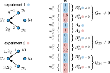
Figure 2: An example of $\mathbf{w}$ in the setup of multiple experiments.

Let us introduce a term of group sparsity based on $\mathbf{w}$,

$$\mathbf{w}^{S}\coloneqq\big{[}\|\mathbf{w}_{1}\|_{2},\;\cdots,\;\|\mathbf{w}_{M}\|_{2}\big{]}^{T},$$ (17)

where $\|\cdot\|_{2}$ denotes the $l_{2}$-norm of vectors and $M$ is the number of groups/blocks in (14). The dimensions of each block $\mathbf{w}_{k}^{[l]}$ and $\mathbf{w}_{k}$ in (15) are saved in two vectors $\rho^{E}$ and $\rho^{S}$, respectively

$$\begin{array}[]{ll}&\rho\triangleq\big{[}n_{i1}^{by},\dots,n_{i}^{a},\dots,n_{ip}^{by},n_{i1}^{bu},\dots,n_{ip}^{bu},n_{i}^{c}\big{]}^{T},\\ &\rho^{E}\coloneqq\rho\otimes\mathbf{1}_{L},\qquad\rho^{S}\coloneqq L\rho,\end{array}$$ (18)

where the elements of $\rho$ are defined with respect to (10), $\mathbf{1}_{L}$ is a $L$-dimensional column vector of $1$’s, and the index $i$ in $\rho$ indicates the regression problem for $y_{i}$, as assumed by default.

Group sparsity is demanded to guarantee networks sparsity and that the network structure is consistent over replica (i.e. the interconnection structure determined by the $\mathbf{w}^{[l]}$’s are identical for all $l$). The sparsity is imposed on each large group $\mathbf{w}_{k}$, $k=1,\dots,M$, and the penalty term is $\lambda\|\mathbf{w}^{S}\|_{0}$, where $\lambda\in\mathbb{R}^{+}$. The mechanism on how group sparsity functions is described as follows.

Recall that the setup (16) allows the system parameters to be different in values for different $l$’s. Note that each small block $\mathbf{w}_{k}^{[l]}$ corresponds to an arc in the underlying digraph of the dynamical system in the $l$-th experiment (e.g., see Fig. 2). The $\|\mathbf{w}_{k}\|_{2}$ chosen to be zero yields that all $\mathbf{w}_{k}^{[l]},l=1,\dots,L$ are equal to zeros. It implies that the arc corresponding to $\mathbf{w}_{k}^{[l]}$ does not exist in dynamic networks for any $l$. In addition, thanks to the effect of noise, it is nearly guaranteed that $\mathbf{w}_{k}^{[l]}$ is not identical to zero for almost all $l$ if $\|\mathbf{w}_{k}\|_{2}\neq 0$. This is how the group sparsity (defined via $\mathbf{w}^{S}$) guarantees that the resultant networks of different datasets share the same topology. Moreover, when a classical least squares objective is augmented with a penalty term of $\lambda\|\mathbf{w}^{S}\|_{0}$, the optimal solution favors zeros of $\mathbf{w}_{k},k=1,\dots,M$, which guarantees the sparsity of network structures. In summary, to perform network reconstruction from heterogeneous datasets, we solve the following optimization problem

$$\underset{\mathbf{w}}{\operatorname{minimize}\;}\|\mathbf{y}-\mathbf{A}(\mathbf{w})\mathbf{w}\|^{2}+\lambda\|\mathbf{w}^{S}\|_{0},$$ (19)

where the norm $\|\cdot\|$ can be simply the $l_{2}$-norm in the classic $l_{1}$ methods (see Section 5.1), or the $l_{2}$-norm weighted by inverse noise covariance $\Sigma^{-1}$ of $\boldsymbol{\xi}$ in (16), as specified in details later in Section 5.2 and 5.3.

5 Methods for structured group sparsity

The problem of network reconstruction from heterogeneous data has been tackled in Section 3 and 4, which results in an regularised optimisation problem. The onus is to solve the group sparsity problem (19) provided with the fixed partition given in (15). However, subject to the progress of regularised optimisation, this section focuses on handling the ARX, or any other parametrization that results in (19) being a regularised linear least square problem. Indeed, there could be heuristic methods to solve the general (19), due to lack of rigorousness in mathematics, which will not be covered in this paper. We organise this section as a separate module such that any solver that readers trust could be integrated with Section 3 and 4 to solve reconstruction problems from multiple experiments.

5.1 Classic $l_{1}$ methods

Two well-known methods are firstly introduced and extended to solve the “linear case” of (19), specifically, classic $l_{1}$ heuristic methods and sparse Bayesian learning (SBL). The classic $l_{1}$ methods refer to the family of methods that use best convex approximation of (19). Due to the general sparsity structure of $\mathbf{w}^{S}$, the resultant problem will have a more general form than the standard group LASSO in [30]. The extended formulations of $l_{1}$ methods for structured group sparsity will be presented, together with an ADMM algorithm for large-scale problems.

5.1.1 Convex approximation

As addressed in Section 3.2, choosing ARX to parametrize network models results in a linear regression, in which $\mathbf{A}$ does not depend on $\mathbf{w}$ in (16). The treatment of classical group LASSO yields

$$\underset{\mathbf{w}}{\operatorname{minimize}\;}\|\mathbf{y}-\mathbf{A}\mathbf{w}\|_{2}^{2}+\lambda\|\mathbf{w}^{S}\|_{1},$$ (20)

where

$$\|\mathbf{w}^{S}\|_{1}=\sum_{i=1}^{M}\sqrt{\rho_{i}^{S}}\|\mathbf{w}_{i}\|_{2},$$ (21)

and $\lambda\in\mathbb{N}_{+}$. This is a convex optimization and has been soundly studied (e.g., [31]). To achieve a better approximation of the $l_{0}$-norm, alternatively one may use iterative reweighted $l_{1}/l_{2}$ methods (e.g. see [32, 33]). Applying to group sparsity, both methods turn to a similar scheme (differing in the usage of $\|\cdot\|_{2}$ or $\|\cdot\|^{2}_{2}$ for blocks of $\mathbf{w}$ in (22) and (23)). Here we present the solution using the $l_{1}$ method,

$$\mathbf{w}^{(k+1)}=\operatorname{arg}\,\!\underset{\mathbf{w}}{\operatorname{min}}\;\|\mathbf{y}-\mathbf{Aw}\|_{2}^{2}+\lambda\sum_{i=1}^{M}\nu_{i}^{(k)}\sqrt{\rho_{i}^{S}}\|\mathbf{w}_{i}\|_{2},$$ (22)

where

$$\nu_{i}^{(k)}=\Big{[}\|\mathbf{w}_{i}^{(k)}\|_{2}+\epsilon^{(k)}\Big{]}^{-1}$$ (23)

and $k$ is the index of iterations. In regard to the selection of $\epsilon$, $\{\epsilon^{(k)}\}_{k=1,2,\dots}$ should be a sequence converging to zero, as addressed in [33] based on the Unique Representation Property. It suggests in [33] a fairly simple update rule of $\epsilon$, i.e. $\epsilon^{(k)}\in(0,1)$ is reduced by a factor of 10 until reaching a minimum of $10^{-8}$ (the factor and lower bound could be tuned specifically). One may also adopt an adaptive rule of $\epsilon$ given in [32].

5.1.2 ADMM for large-scale problems

To solve the convex optimization in Section 5.1.1, for example, CVX for MATLAB could be an easy solution. However, the computation time could be enormous for large-dimension problems. This section presents algorithms using proximal methods and ADMM ([34]) to handle large-dimension network reconstruction.

Let us first consider (20), which is rewritten as

$$\underset{\mathbf{w}}{\operatorname{minimize}\;}f(\mathbf{w})+g(\mathbf{w}),$$ (24)

where $f(\mathbf{w})\triangleq(1/2)\|\mathbf{y}-\mathbf{A}\mathbf{w}\|_{2}^{2}$, $g(\mathbf{w})\triangleq\lambda\|\mathbf{w}^{S}\|_{1}$, $\lambda$ is twice larger than the value in (21). Given $\nabla f(\mathbf{w})=\mathbf{A}^{T}(\mathbf{A}\mathbf{w}-\mathbf{y})$, the proximal gradient method is to update $\mathbf{w}$ by $\mathbf{w}^{(k+1)}=\mathbf{prox}_{\gamma g}(\mathbf{w}^{(k)}-\gamma\nabla f(\mathbf{w}^{(k)})),\,\gamma\in\mathbb{R}_{+}$, where $k$ is the iteration index and $\mathbf{prox}_{f}(\cdot)$ denotes the standard proximal operator of function $f$ (see [34, 35]). It is easy to see that $g(\mathbf{w})=\sum_{i=1}^{N}g_{i}(\mathbf{w}_{i})$, where $g_{i}(\mathbf{w}_{i})\triangleq\lambda\sqrt{\rho_{i}^{S}}\|\mathbf{w}_{i}\|_{2}$. Firstly we partition the variable $\mathbf{v}$ of $\mathbf{prox}_{\gamma g}(\mathbf{v})$ in the same way as $\mathbf{w}$ in terms of $\mathbf{w}_{i},i=1,\dots,M$, i.e. $\mathbf{v}=[\mathbf{v}_{1}^{T},\dots,\mathbf{v}_{M}^{T}]^{T}$. Then we calculate the proximal operator $\mathbf{prox}_{\gamma g_{i}}(\mathbf{v}_{i})$, which equals

$$\mathbf{prox}_{\gamma g_{i}}(\mathbf{v}_{i})=\Big{(}1-\gamma\lambda\sqrt{\rho_{i}^{S}}/\|\mathbf{v}_{i}\|_{2}\Big{)}_{+}\mathbf{v}_{i},$$ (25)

where $(\cdot)_{+}$ replaces each negative elements with 0. It follows that

$$\mathbf{prox}_{\gamma g}(\mathbf{v})=\begin{bmatrix}\left(\mathbf{prox}_{\gamma g_{1}}(\mathbf{v}_{1})\right)^{T}&\cdots&\left(\mathbf{prox}_{\gamma g_{M}}(\mathbf{v}_{M})\right)^{T}\end{bmatrix}^{T}.$$ (26)

The value of $\gamma$ needs to be selected appropriately so as to guarantee the convergence. One simple solution is using line search methods, e.g., see Section 4.2 in [34].

Provided with the above calculations, it is straightforward to implement the (accelerated) proximal gradient method (see [34, chap. 4.3]). To implement ADMM, the proximal operator of $f(\mathbf{w})$ needs to be calculated,

$$\mathbf{prox}_{\gamma f}(\mathbf{v})=(I+\gamma\mathbf{A}^{T}\mathbf{A})^{-1}(\gamma\mathbf{A}^{T}\mathbf{y}+\mathbf{v}).$$ (27)

Given $\mathbf{prox}_{\gamma g}(\mathbf{v})$ as (25) and (26), the ADMM method is presented in Algorithm 1.

Algorithm 1 ADMM method

1:Precompute $\mathbf{A}^{T}\mathbf{A}$ and $\mathbf{A}^{T}\mathbf{y}$

2:given an initial value $\mathbf{w}^{0},\mathbf{z}^{0},\mathbf{u}^{0}$, $\gamma^{0}=1$, and $\beta=1/2$

3:repeat

4:     $\gamma\leftarrow\gamma^{(k)}$

5:     repeat

6:         $\hat{\mathbf{w}}\leftarrow\mathbf{prox}_{\gamma f}(\mathbf{z}^{(k)}-\mathbf{u}^{(k)})$ using (27)

7:         break if $f(\hat{\mathbf{w}})\leq f(\mathbf{w}^{(k)})+\nabla f(\mathbf{w}^{(k)})^{T}(\hat{\mathbf{w}}-\mathbf{w}^{(k)})+(1/2\gamma)\|\hat{\mathbf{w}}-\mathbf{w}^{(k)}\|_{2}^{2}$

8:         $\gamma\leftarrow\beta\gamma$

9:     until ;

10:     $\mathbf{w}^{(k+1)}\leftarrow\hat{\mathbf{w}}$, $\gamma^{(k+1)}\leftarrow\gamma$

11:     Compute $\mathbf{prox}_{\gamma g_{i}}(\mathbf{w}^{(k+1)}_{i}+\mathbf{u}^{(k)}_{i})$ by (25) for $i=1,...,M$

12:     $\mathbf{z}^{(k+1)}\leftarrow\mathbf{prox}_{\gamma g}(\mathbf{w}^{(k+1)}+\mathbf{u}^{(k)})$ using (26)

13:     $\mathbf{u}^{(k+1)}\leftarrow\mathbf{u}^{(k)}+\mathbf{w}^{(k+1)}-\mathbf{z}^{(k+1)}$

14:until any standard stopping criteria

To use this algorithm for the iterative reweighted $l_{1}$ method (22), we only need to modify (25), which now should be

$$\mathbf{prox}_{\gamma g_{i}}(\mathbf{v}_{i})=\Big{(}1-\gamma\lambda\nu_{i}\sqrt{\rho_{i}^{S}}/\|\mathbf{v}_{i}\|_{2}\Big{)}_{+}\mathbf{v}_{i}.$$ (28)

In each “outer” loop indicated by (22), we update $\nu_{i}$ by (23) and implement ADMM as Algorithm 1 to solve (22).

5.2 Sparse Bayesian learning

Another method is sparse Bayesian learning, which was originally proposed in [36] to heuristically acquire sparsity. Its effectiveness and performance are further analysed in [37] and compared to the iterative reweighted $l_{1}/l_{2}$ methods in theory in [38]. Our problem demands a more general form of group sparsity and noise covariance structures than that specified in [39]. It includes how to structure priors to match the specification of $\mathbf{w}^{S}$ and an extended EM algorithm for generalised noise covariance structures.

Consider

$$\mathbf{y}=\mathbf{A}\mathbf{w}+\boldsymbol{\xi},\quad\boldsymbol{\xi}\sim\mathcal{N}(0,\Sigma),$$ (29)

where $\Sigma=\operatorname{{diag}}(\sigma_{1}^{2}I_{1},\dots,\sigma_{L}^{2}I_{L})$ with $\sigma_{l}\in\mathbb{R}_{+}$; identity matrix $I_{l}$ is of dimension $N_{l}$ (that denotes the length of time series from the $l$-th experiment); $\mathbf{y}$ is of dimension $M_{\mathbf{y}}$; and $\mathbf{w}$ is of dimension $M_{\mathbf{w}}$ (it is easy to see $M_{\mathbf{y}}=\sum_{l=1}^{L}N_{l}$ and $N_{\mathbf{w}}=\|\rho^{S}\|_{1}$ from (13) and (17)). Most SBL papers (e.g., [36, 38, 39, 37]) consider a simple form of noise variance $\Sigma=\sigma^{2}I$, which may fail to be a fair approximation in our study if noise variances in different experiments are significantly different. This section will extend SBL to handle different group sizes and diagonal noise variance matrices.

5.2.1 Model prior formulation

Suppose the automatic relevance determination (ARD) prior [36, 37] in SBL is given as

$$p(\mathbf{w};\Gamma)=\frac{1}{(2\pi)^{M_{\mathbf{w}}/2}|\Gamma|^{1/2}}\exp\left(-\frac{1}{2}\mathbf{w}^{T}\Gamma^{-1}\mathbf{w}\right).$$ (30)

In regard to hyperparameter $\Gamma$, we will enforce a specific structure empirically to impose group sparsity. For each $\mathbf{w}_{j}$, $j=1,\dots,M$,

$$p(\mathbf{w}_{j};\gamma_{j})=\mathcal{N}(0,\gamma_{j}I_{j}),\;\;p(\mathbf{w};\boldsymbol{\gamma})=\prod_{j=1}^{M}p(\mathbf{w}_{j};\gamma_{j}),$$ (31)

where $\gamma_{j}\in\mathbb{R}_{+}$, $I_{j}$ is a $LM_{j}\!\times\!LM_{j}$ identity matrix,

$$M_{j}=\begin{cases}n_{ij}^{by}&\text{if }1\leq j\leq p\text{ and }j\neq i,\\ n_{i}^{a}&\text{if }j=i,\\ n_{ij}^{bu}&\text{if }p+1\leq j\leq p+m=M,\\ \end{cases}$$ (32)

the index $i$ in (32) indicates that we are dealing with the $i$-th output (see (10), (12)), and $\boldsymbol{\gamma}\triangleq[\gamma_{1},\dots,\gamma_{M}]^{T}$. Therefore, $\Gamma$ is constructed as

$$\Gamma=\operatorname{{diag}}\big{(}\gamma_{1}I_{1},\cdots,\gamma_{M}I_{M}\big{)}.$$ (33)

For simplicity, we will interchangeably use two notations for the prior $p(\mathbf{w};\Gamma)\triangleq p(\mathbf{w};\boldsymbol{\gamma}).$

5.2.2 Parameter estimation

The likelihood function of (29) is Gaussian,

$$p(\mathbf{y}\mid\mathbf{w};\Sigma)=\left(2\pi\right)^{-\frac{M_{\mathbf{y}}}{2}}|\Sigma|^{-\frac{1}{2}}\exp\left(\|\mathbf{y}-\mathbf{A}\mathbf{w}\|_{\Sigma^{-1}}^{2}\right).$$ (34)

The hyperparameters $\boldsymbol{\gamma}$, along with the error variance $\Sigma$ can be estimated from data by evidence maximisation (or called type-II maximum likelihood), i.e. marginalising over the weights $\mathbf{w}$ and then perform maximum likelihood. The marginalised probabilistic density function can be analytically calculated

$$\begin{array}[]{ll}p(\mathbf{y};\boldsymbol{\gamma},\Sigma)&\displaystyle=\int p(\mathbf{y}\mid\mathbf{w};\Sigma)p(\mathbf{w};\boldsymbol{\gamma})\mathrm{d}\mathbf{w}\\ &\displaystyle=\frac{1}{(2\pi)^{M_{\mathbf{y}}/2}|\Sigma_{\mathbf{y}}|^{1/2}}\exp\left(-\frac{1}{2}\mathbf{y}^{T}\Sigma_{\mathbf{y}}^{-1}\mathbf{y}\right),\end{array}$$ (35)

where $\Sigma_{\mathbf{y}}\triangleq\Sigma+\mathbf{A}\Gamma\mathbf{A}^{T}$. With fixed values of the hyperparameters, the posterior density is Gaussian, i.e.

$$p(\mathbf{w}\mid\mathbf{y};\boldsymbol{\gamma},\Sigma)=\mathcal{N}(\boldsymbol{\mu},\Sigma_{\mathbf{w}})$$ (36)

with $\boldsymbol{\mu}=\Sigma_{\mathbf{w}}\mathbf{A}^{T}\Sigma^{-1}\mathbf{y}$ and $\Sigma_{\mathbf{w}}=\left(\mathbf{A}^{T}\Sigma^{-1}\mathbf{A}+\Gamma^{-1}\right)^{-1}$. Once we have $\boldsymbol{\gamma}$ and $\Sigma$ estimated via type-II maximum likelihood, we can choose our weights $\hat{\mathbf{w}}$ via

$$\hat{\mathbf{w}}=\boldsymbol{\mu}=\left(\mathbf{A}^{T}\Sigma_{\mathrm{ML}}^{-1}\mathbf{A}+\Gamma_{\mathrm{ML}}^{-1}\right)^{-1}\mathbf{A}^{T}\Sigma^{-1}_{\mathrm{ML}}\mathbf{y}.$$ (37)

5.2.3 Algorithms

There are several ways to compute ${\Gamma}_{\mathrm{ML}}$ and $\Sigma_{\mathrm{ML}}$: expectation maximization (EM) in [37], fixed-point methods in [36], and difference of convex program (DCP) in [24]. Here we introduce the EM approach and the others can be similarly derived.

The EM method proceeds by treating the weights $\mathbf{w}$ as hidden variables and then maximizing

$$\mathbb{E}_{\mathbf{w}|\mathbf{y};\boldsymbol{\gamma},\Sigma}\,\big{[}p(\mathbf{y},\mathbf{w};\boldsymbol{\gamma},\Sigma)\big{]},$$

where $p(\mathbf{y},\mathbf{w};\boldsymbol{\gamma},\Sigma)=p(\mathbf{y}|\mathbf{w};\Sigma)p(\mathbf{w};\boldsymbol{\gamma})$ is the likelihood of the complete data $\{\mathbf{w},\mathbf{y}\}$. The whole EM algorithm for the extended SBL is summarized as follows: given the estimates $\boldsymbol{\gamma}^{(k)}$ and $\Sigma^{(k)}$, at the ($k\!+\!1$)-th iterate,

• E-step: $\mathbb{E}_{\mathbf{w}|\mathbf{y};\boldsymbol{\gamma}^{(k)},\Sigma^{(k)}}(\mathbf{w}_{i}^{2})=\left(\Sigma_{\mathbf{w}}\right)_{i,i}+\boldsymbol{\mu}_{i}^{2}.$

• M-step:

  $$\begin{array}[t]{@{}lrll}&\boldsymbol{\gamma}^{(k+1)}&=&\underset{\boldsymbol{\gamma}\geq 0}{\operatorname{arg\,\!max}\;}\mathbb{E}_{\mathbf{w}|\mathbf{y};\boldsymbol{\gamma}^{(k)},\Sigma^{(k)}}\big{[}p(\mathbf{y},\mathbf{w};\boldsymbol{\gamma},\Sigma^{(k)}\big{]}\\ \Rightarrow&\gamma_{j}^{(k+1)}&=&\frac{1}{LM_{j}}\sum_{i\in\Lambda_{j}}\left[\boldsymbol{\mu}_{i}^{2}+(\Sigma_{\mathbf{w}})_{i,i}\right],\\[5.0pt] &\Sigma^{(k+1)}&=&\operatorname{arg}\,\!\underset{\Sigma>0}{\operatorname{max}}\;\mathbb{E}_{\mathbf{w}|\mathbf{y};\boldsymbol{\gamma}^{(k)},\Sigma^{(k)}}\big{[}p(\mathbf{y},\mathbf{w};\boldsymbol{\gamma}^{(k)},\Sigma)\big{]}\\ \Rightarrow&(\sigma_{l}^{2})^{(k+1)}&=&\frac{1}{N_{\mathbf{y}}}\big{\{}\|\mathbf{y}^{[l]}-\mathbf{A}^{[l]}\boldsymbol{\mu}\|^{2}+\\ &&&(\sigma_{l}^{2})^{(k)}\sum_{i=1}^{M_{\mathbf{w}}}\big{[}1-\big{(}\boldsymbol{\gamma}_{i}^{(k)}\big{)}^{-1}(\Sigma_{\mathbf{w}})_{i,i}\big{]}\big{\}},\end{array}$$

for $j=1,\dots,M$; $i=1,\dots,M_{\mathbf{w}}$; $l=1,\dots,L$ and $\Sigma^{(k+1)}=\operatorname{{diag}}((\sigma_{1}^{2})^{(k+1)}I_{1},\dots,(\sigma_{L}^{2})^{(k+1)}I_{L})$, where $\boldsymbol{\mu}$ and $\Sigma_{\mathbf{w}}$ are calculated via (36) provided with $\boldsymbol{\gamma}^{(k)}$ and $\Sigma^{(k)}$, $M_{j}$ is given in (32) and $\Lambda_{j}$ denotes the row (column) indexes associated with $\gamma_{j}$ in $\Gamma$.

5.3 Sparse estimation via sampling

This section will propose an approach based on sampling methods for sparse estimation, which is powerful to handle small data and has more flexibility to be extended. This idea is inspired by the work in Monte Carlo strategies for binary variables, e.g., [40] for model selection, or sampling methods for Ising and Potts models in statistical physics (e.g., see [41]). The sampling methods will be used in this section to estimate the underlying sparse structures. Note that this approach does not heuristically enforce sparsity as the $l_{1}$ methods or SBL does.

Consider

$$\mathbf{y}=\mathbf{A}\mathbf{w}+\boldsymbol{\xi},\quad\boldsymbol{\xi}\sim\mathcal{N}(0,\Sigma),$$ (38)

where $\Sigma=\operatorname{{diag}}(\sigma_{1}^{2}I_{1},\dots,\sigma_{L}^{2}I_{L})$ with $\sigma_{l}\in\mathbb{R}_{+}$; identity matrix $I_{l}$ is of dimension $N_{l}$ (that denotes the length of time series from the $l$-th experiment); $\mathbf{y}$ is of dimension $M_{\mathbf{y}}$; and $\mathbf{w}$ is of dimension $M_{\mathbf{w}}$ (it is easy to see $M_{\mathbf{y}}=\sum_{l=1}^{L}N_{l}$ and $N_{\mathbf{w}}=\|\rho^{S}\|_{1}$ from (13) and (17)). Hence, the likelihood of (38) is Gaussian, given as

$$p(\mathbf{y}\mid\mathbf{w};\Sigma)=\left(2\pi\right)^{-\frac{M_{\mathbf{y}}}{2}}|\Sigma|^{-\frac{1}{2}}\exp\left(-\frac{1}{2}\|\mathbf{y}-\mathbf{A}\mathbf{w}\|_{\Sigma^{-1}}^{2}\right).$$ (39)

The key that allows sparse estimation via sampling is to introduce a “virtual” variable $\mathbf{s}\triangleq[s_{1},\dots,s_{M}]$ to describe the underlying sparse structure of $\mathbf{w}$, defined by

$$\mathbf{w}=\operatorname{{diag}}(s_{1}I_{1},\dots,s_{M}I_{M})\boldsymbol{\vartheta}\triangleq S\boldsymbol{\vartheta},$$ (40)

where indicator variables $s_{i}\in\{0,1\}$, each identity matrix $I_{i}$ ($i=1,\dots,M$) is of dimension specified by $\rho^{S}$ in (18) correspondingly, and $\boldsymbol{\vartheta}\in\mathbb{R}^{M_{\mathbf{w}}}$. Now the idea becomes clear that, as sampling the atomic spins in the Ising model, sampling $\mathbf{s}$ from any posterior distribution tells the sparsity structure of $\mathbf{w}$. There could be multiple choices of priors for $\mathbf{s}$. Here we suggest the Bernoulli distribution, given as $\mathbf{s}\sim\prod_{i=1}^{M}\mathcal{B}(1,p_{i})$ ($p_{i}\in(0,1)$, e.g., $p_{i}=1/2$). And the prior for $\boldsymbol{\vartheta}$ is chosen to be Gaussian,

$$p(\boldsymbol{\vartheta};\Gamma)=(2\pi)^{-\frac{M_{\mathbf{w}}}{2}}|\Gamma|^{-\frac{1}{2}}\exp\left(-\frac{1}{2}\boldsymbol{\vartheta}^{T}\Gamma^{-1}\boldsymbol{\vartheta}\right).$$ (41)

The covariance structure of $\Gamma$ could either be simply $\Gamma=\gamma I$ or be diagonal $\Gamma=\operatorname{{diag}}(\gamma_{1}I_{1},\dots,\gamma_{M}I_{M})$, in which $I_{i}$ ($i=1,\dots,M$) is the same as (40). Letting $\boldsymbol{\gamma}\triangleq(\gamma_{1},\dots,\gamma_{M})$, for brevity, we will use $\Gamma$ and $\boldsymbol{\gamma}$ interchangeably. Furthermore, we use the inverse Gamma distribution as the hyperprior independently for each $\sigma^{2}_{l}$ ($l=1,\dots,L$) or ${\gamma_{i}}$ ($i=1,\dots,M$) (e.g., see [42]), denoted by $\sigma^{2}_{l}\sim\mathcal{G}^{-1}(a,b)$ and ${\gamma_{i}}\sim\mathcal{G}^{-1}(c,d)$, where $a,b,c,d$ choose small values (e.g., $10^{-4}$) to make these hyperprior non-informative.

Since $\boldsymbol{\vartheta}$ is a multivariate continuous variable, sampling $\boldsymbol{\vartheta}$ could be particularly costly for large dimensions. Instead, we perform a “collapse” operation on the posterior distribution [43], and sample $\mathbf{s}$ from the marginalised posterior to determine the sparse structure. The estimation of $\mathbf{w}$ could be performed at the end by running a linear regression with its sparsity structure specified. The posterior $p(\mathbf{s},\boldsymbol{\vartheta},\boldsymbol{\gamma},\Sigma\mid\mathbf{y})$ is marginalised over $\boldsymbol{\vartheta}$,

$$\begin{array}[]{l@{\:}l}p(\mathbf{s},\boldsymbol{\gamma},\Sigma\mid\mathbf{y})\hfil\>&\propto\displaystyle p(\mathbf{s})p(\boldsymbol{\gamma})p(\Sigma)p(\mathbf{y}\mid\mathbf{s},\Sigma,\boldsymbol{\gamma}),\\ \hfil\>&\propto\displaystyle p(\mathbf{s})p(\boldsymbol{\gamma})p(\Sigma)\int p(\mathbf{y}\mid\mathbf{w},\Sigma)p(\boldsymbol{\vartheta}\mid\boldsymbol{\gamma})\mathrm{d}\boldsymbol{\vartheta}.\end{array}$$ (42)

Substituting the priors and completing squares, it yields

$$p(\mathbf{y}\mid\mathbf{s},\Sigma,\boldsymbol{\gamma})=(2\pi)^{-\frac{M_{\mathbf{y}}}{2}}\left|\Sigma_{\mathbf{y}}\right|^{-\frac{1}{2}}\exp\left(-\frac{1}{2}\|\mathbf{y}\|_{\Sigma_{\mathbf{y}}^{-1}}^{2}\right),$$ (43)

where

$$\Sigma_{\mathbf{y}}=\Sigma+\mathbf{A}S\Gamma S\mathbf{A}^{T}.$$ (44)

The onus is to sample $\mathbf{s},\Sigma$ and $\boldsymbol{\gamma}$ from $p(\mathbf{s},\boldsymbol{\gamma},\Sigma\mid\mathbf{y})$. The Metropolis-Hastings algorithm within the systematic-scan Gibbs sampler (e.g., see [41]) will be used to draw samples. Suppose that the $k$-th samples $\mathbf{s}^{(k)},\boldsymbol{\gamma}^{(k)}$ and $\Sigma^{(k)}$ have been available. At the $k+1$ iteration,

• draw $\mathbf{s}^{(k+1)}$ from the conditional distribution
  $p(\mathbf{s}\mid\mathbf{y},\boldsymbol{\gamma}^{(k)},\Sigma^{(k)})$,

• draw $\boldsymbol{\gamma}^{(k+1)}$ from $p(\boldsymbol{\gamma}\mid\mathbf{y},\mathbf{s}^{(k+1)},\Sigma^{(k)})$, and

• draw $\Sigma^{(k+1)}$ from $p(\Sigma\mid\mathbf{y},\mathbf{s}^{(k+1)},\boldsymbol{\gamma}^{(k+1)})$.

In each sampling step, we use the Metropolis-Hastings algorithm. Consider drawing samples from $p(\mathbf{s}\mid\mathbf{y},\boldsymbol{\gamma},\Sigma)$, in which the key is to choose a proposal distribution $T(\mathbf{s}^{(k)},\hat{\mathbf{s}})$, where $\mathbf{s}^{(k)}$ is a given sample and $\hat{\mathbf{s}}$ is a new configuration. Here we use a simple scheme that gives a symmetric proposal distribution (i.e. $T(\mathbf{s}^{(k)},\hat{\mathbf{s}})=T(\hat{\mathbf{s}},\mathbf{s}^{(k)})$). We randomly pick an element of $\mathbf{s}^{(k)}$ and flip it, i.e. draw $\hat{i}$ from the uniform distribution on $\{1,\dots,M\}$ and set $\hat{s}_{i}$ to be equal to $s_{i}^{(k)}$ if $i\neq\hat{i}$ and $1-s_{i}^{(k)}$ otherwise. The Metropolis-Hastings algorithm for $p(\mathbf{s}\mid\mathbf{y},\boldsymbol{\gamma},\Sigma)$ is given as below: given $\boldsymbol{\gamma}^{(k)},\Sigma^{(k)}$ and $\mathbf{s}^{(k)}$,

• draw $\hat{\mathbf{s}}$ from the proposal distribution $T(\mathbf{s}^{(k)},\hat{\mathbf{s}})$ using the above scheme;

• draw $U\sim\text{Uniform}[0,1]$ and update

  $$\begin{array}[]{r@{\:}l}\>&\mathbf{s}^{(k+1)}=\begin{cases}\hat{\mathbf{s}},&\text{if }U\leq r(\mathbf{s}^{(k)},\hat{\mathbf{s}})\\ \mathbf{s}^{(k)},&\text{otherwise}\end{cases},\;\;\text{with}\\[10.0pt] \>&r(\mathbf{s}^{(k)},\hat{\mathbf{s}})=\min\displaystyle\left\{1,\frac{p(\hat{\mathbf{s}},\boldsymbol{\gamma}^{(k)},\Sigma^{(k)}\mid\mathbf{y})T(\hat{\mathbf{s}},\mathbf{s}^{(k)})}{p(\mathbf{s}^{(k)},\boldsymbol{\gamma}^{(k)},\Sigma^{(k)}\mid\mathbf{y})T(\mathbf{s}^{(k)},\hat{\mathbf{s}})}\right\}.\end{array}$$

In regard to the Metropolis-Hastings algorithms for $\boldsymbol{\gamma}$ and $\Sigma$, we use random walk sampling $\hat{\boldsymbol{\gamma}}=\boldsymbol{\gamma}^{(k)}+\mathbf{u},\hat{\Sigma}=\Sigma^{(k)}+\operatorname{{diag}}(v_{1}I_{1},\dots,v_{L}I_{L})$, where $\mathbf{u}$ and ${v_{i}}$ are normally distributed with mean zero and fixed variances (which may need to be tuned to have sound convergence speeds and acceptance ratios), and the acceptance probabilities are given as, respectively,

$$r(\boldsymbol{\gamma}^{(k)},\hat{\boldsymbol{\gamma}}) =\min\left\{1,\frac{p(\mathbf{s}^{(k+1)},\hat{\boldsymbol{\gamma}},\Sigma^{(k)}\mid\mathbf{y})}{p(\mathbf{s}^{(k+1)},\boldsymbol{\gamma}^{(k)},\Sigma^{(k)}\mid\mathbf{y})}\right\},$$

$$r({\Sigma}^{(k)},\hat{\Sigma}) =\min\left\{1,\frac{p(\mathbf{s}^{(k+1)},\boldsymbol{\gamma}^{(k+1)},\hat{\Sigma}\mid\mathbf{y})}{p(\mathbf{s}^{(k+1)},\boldsymbol{\gamma}^{(k+1)},\Sigma^{(k)}\mid\mathbf{y})}\right\}.$$

6 Numerical examples

This section presents several Monte Carlo studies to show inference performance from multiple experiments. It first applies three sparsity techniques in the proposed method for multiple experiments, presented in Section 3 & 4. To further show the superiority of simultaneous processing of multiple-experiment data, we provide two more studies that compare the proposed method with the “naive” treatment (i.e. inferring networks separately from each dataset, and then choosing the edges in common) widely used in applications.

ARX networks refer to such a class of discrete-time DSF models (2) that each MISO transfer function (3) can be exactly rewritten as an ARX model. To randomly generate proper signals for benchmarking, it is further required that these random ARX networks should be stable (see [44] or [45]; or only demanding BIBO stability) and have sparse network structures that should not be oversimplified (e.g., trees or acyclic digraphs may not be satisfactory). This is particularly challenging due to the demands on both sparse structures (with loops) and stability. Here we propose a simplified strategy for random model generation, whose details are provided in the supplement [26, app. C] for interested readers. The basic idea is to repetitively apply the small gain theorem in sequence so as to stabilise the whole ARX network. Moreover, to generate its replica models for multiple experiments (i.e. models with $L>1$), we randomly perturb its nonzero model parameters and/or noise covariance. Due to technical issues in model generation, the perturbation remains relatively minor to avoid triggering network instability.

The performance indexes for benchmarks use the precision (Prec) and the true positive rate (TPR), defined as $\text{Prec}={\text{TP}}/{(\text{TP}+\text{FP})}$ and $\text{TPR}={\text{TP}}/{(\text{TP}+\text{FN})}$, where TP (true positive), FP (false positive) and FN (false negative) are the standard concepts in the Receiver Operating Characteristic (ROC) curve or the Precision Recall curve (e.g. see [46]). One may understand Prec as the percentage of correct arcs in the inferred network, and TPR as the percentage of correctly inferred arcs in the ground truth. The ideal is to achieve both high values, while, if not possible, Prec has higher priority since its low value results in completely useless inference.

The benchmark study, as shown in Fig. 3 (and Table 1 in the supplement [26]), performs the proposed reconstruction method for randomly generated data, equipped with iterative reweighted $l_{1}$ method (labeled as “GIRL1”), sparse Bayesian learning (labeled as “GSBL”) and the sampling method (labeled as “GSMC” ) for group sparsity. There are two test scenarios: 1) models with $p=10$ (i.e. $\#\text{nodes}=10$) and different SNRs ($\text{SNR}=0,10,20,40$ dB); 2) models with $\text{SNR}=10$ dB and different number of nodes $p=5,10,15,20$. Each test (with given $p$ and SNR) generates $50$ random stable ARX networks and simulates time series of length $1000$. All models are set to the same sparsity density $0.2$, i.e. the total number of nonzero entries in $Q$ is $0.2p^{2}$. The input signals are independently and identically distributed Gaussian noise with zero mean and unit variance. In the test of GIRL1, the regularization parameter $\lambda$ is set to as follows: $\lambda=0.1,0.1,0.01,0.001$ for $\text{SNR}=0,10,20,40\text{dB}$, respectively; and $\lambda=0.05,0.1,0.1,0.1$ for $p=5,10,15,20$. The parameter $\lambda$ is chosen roughly among values in logarithmic scales for one model by reviewing the sparsity density of the inference results (assuming we roughly know how sparse the network should be), and then is used for all 50 models. One certainly can apply cross-validation or bootstrap methods to choose and tailor $\lambda$ for every model for better performance.

The comparative results in Fig. 3 tell that GSMC overall outperform in terms of balance between Prec and TPR. And the users are free from tuning regularisation parameters as required in GIRL1 or other regularisation methods. Moreover, GSMC turns to be impressively powerful when time series of limited lengths are available, whereas GIRL1 and GSBL could fail completely. However, the computational cost might increase dramatically when the problem scale increases. We strongly suggest GSMC when problem scales are not too large or the length of time series is particularly limited. The superiority of GIRL1 (or group LASSO) could be the freedom of tuning regularisation parameters, which allows us to heuristically handle large model certainties or non-Gaussian noises in practice. And when the Prec and TPR cannot be both satisfactory, a conservative choice of $\lambda$ helps to improve Prec at the expense of TPR in order to ensure inferred edges being reliable. This explains, in Fig. 3, GIRL1 has better performance on Prec (larger means and smaller variances) than GSBL over different SNRs or #nodes; while the performance on TPR shows slighter weaker than GSBL. This comparison for GSBL shows a slight increase of Prec or TPR when the SNR increases, which, however, is not as significant as our intuition might tell. The reason is that both GSBL and GSMC in theory can handle data with a reasonably large range of SNRs by estimating noise variances reliably.

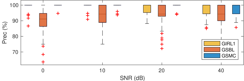
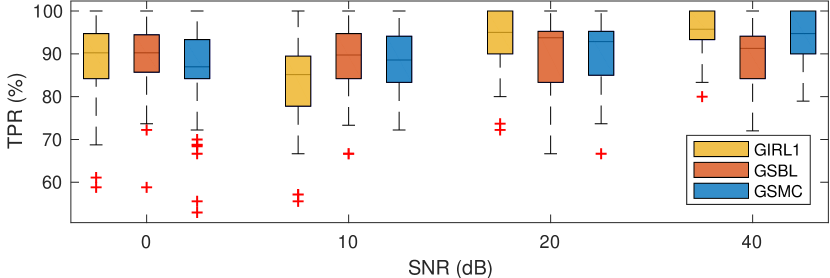
(a) multiple SNRs

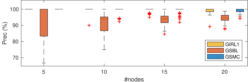
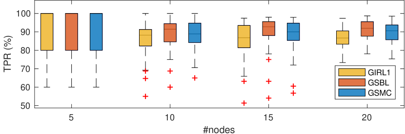
(b) multiple #nodes

Figure 3: Comparative performance of network reconstruction using GIRL1, GSBL and GSMC in scenarios with different SNRs or #nodes.

To further show the superiority of the treatment of heterogeneous data presented in Section 4, we perform two more Monte Carlo studies, in which GSMC is adopted for sparsity. One sets $\text{SNR}=0\text{ dB}$, $L=2$ and prepares time series of length $1000$ for inference. The comparative result in Fig. 4 applies two ways to infer networks for multiple experiments, where one use the proposed method, and the other infers $2$ networks separately from each replica data and then takes intersection of their edge sets. The result shown in Fig. 4 is easy to understand in theory. The intersection gains confidence on the inferred edges, i.e. higher Prec, while sacrificing TPR (its TPR is always equal to or smaller than any TPR of inference from a single replica). In practice, if the diversity between replica data is significant or the number of replica is large, this “naive” treatment becomes very inefficient in the sense that it may miss a large amount of edges that could be explored from data. This is due to approximate methods for sparsity, and thus the heterogeneity of datasets could lead to different topology if processing datasets separately. Another Monte Carlo study manifests that the proposed method could improve both Prec and TPR, as shown in Fig. 5, when single dataset is deficient. It restricts the length of time series to $50$ and sets $L=3$. Fig. 5 shows, by processing three replica data together in the proposed way, we manage to push Prec close to $100\%$ while not affecting TPR or even slightly improving TPR.

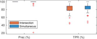
Figure 4: Comparative study of the proposed method (labelled “Simultaneous”) and the “naive” treatment (“Intersection”) to heterogeneous datasets with $L=2$.

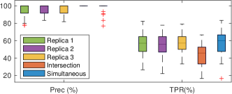
Figure 5: Comparative study to show the superiority of the proposed method to the separate processing of datasets, where $L=3$ and the length of time series is restricted to $50$.

7 Conclusions

This paper discusses dynamic network reconstruction from heterogeneous datasets in the framework of dynamical structure functions (DSFs). It has been addressed that dynamic network reconstruction for linear systems can be formulated as identification of DSFs with sparse structures. To take advantage of heterogeneous datasets from multiple experiments, the proposed method integrates all datasets in one regression form and resorts to group sparsity to guarantee network topology being consistent over replica. To solve the optimisation problem, the treatments using classical convex approximation, SBL and sampling methods have been introduced and extended. The numerical examples manifest the performance of reconstruction from heterogeneous data and reveal practical experience that could guide applications.

This work was supported by Fonds National de la Recherche Luxembourg (Ref. AFR-9247977 and Ref. C14/BM/8231540), and partly supported by the 111 Project on Computational Intelligence and Intelligent Control under Grant B18024.

Appendix A Dynamical structure functions

Consider a dynamical system given by the discrete-time state-space representation in the innovations form

$$\begin{array}[]{l@{\;}l}x(t_{k+1})&=Ax(t_{k})+Bu(t_{k})+Ke(t_{k}),\\ y(t_{k})&=Cx(t_{k})+Du(t_{k})+e(t_{k}),\end{array}$$ (45)

where $x(t_{k})$ and $y(t_{k})$ are real-valued $n$ and $p$-dimensional random variables, respectively; $u(t_{k})\in\mathbb{R}^{m}$, $A,B,C,D,K$ are of appropriate dimensions; and $\{e(t_{k})\}_{k\in\mathbb{N}}$ is a sequence of i.i.d. $p$-dimensional random variables with $e(t_{k})\sim\mathcal{N}(0,R)$. The initial state $x(t_{0})$ is assumed to be a Gaussian random variable with unknown mean $m_{0}$ and variance $R_{0}$. Without loss of generality, we assume $n\geq p$ and $C$ is of full row rank. The procedure to define the DSFs from (45) mainly refers to [15, 27]. Without loss of generality, suppose that $C$ is full row rank (see [27] for a general $C$). Create the $n\!\times\!n$ state transformation $T=\begin{bmatrix}C^{T}&E\end{bmatrix}^{T}$, where $E\in\mathbb{R}^{n\times(n-p)}$ is any basis of the null space of $C$ with $T^{-1}=\begin{bmatrix}\bar{E}&E\end{bmatrix}$ and $\bar{E}=C^{T}(CC^{T})^{-1}$. Now we change the basis such that $z=Tx$, yielding $\hat{A}=TAT^{-1}$, $\hat{B}=TB$, $\hat{C}=CT^{-1}$, $\hat{D}=D$, $K=TK$, and partitioned commensurate with the block partitioning of $T$ and $T^{-1}$ to give

$$\begin{array}[]{r@{\:}c@{\:}l}\begin{bmatrix}z_{1}(t_{k+1})\\ z_{2}(t_{k+1})\end{bmatrix}\>&=\hfil\>&\begin{bmatrix}\hat{A}_{11}&\hat{A}_{12}\\ \hat{A}_{21}&\hat{A}_{22}\end{bmatrix}\begin{bmatrix}z_{1}(t_{k})\\ z_{2}(t_{k})\end{bmatrix}+\begin{bmatrix}\hat{B}_{1}\\ \hat{B}_{2}\end{bmatrix}u(t_{k})+\begin{bmatrix}\hat{K}_{1}\\ \hat{K}_{2}\end{bmatrix}e(t_{k}),\\ y(t_{k})\>&=\hfil\>&\begin{bmatrix}I&0\end{bmatrix}\begin{bmatrix}z_{1}(t_{k})\\ z_{2}(t_{k})\end{bmatrix}+Du(t_{k})+e(t_{k}).\end{array}$$

Introduce the shift operator $q$ and solve for $z_{2}$, yielding $qz_{1}(t_{k})=W(q)z_{1}(t_{k})+V(q)u(t_{k})+L(q)e(t_{k})$, where $W(q)=\hat{A}_{11}+\hat{A}_{12}(qI-\hat{A}_{22})^{-1}\hat{A}_{21}$, $V(q)=\hat{B}_{1}+\hat{A}_{12}(qI-\hat{A}_{22})^{-1}\hat{B}_{2}$, and $L(q)=\hat{H}_{1}+\hat{A}_{12}(qI-\hat{A}_{22})^{-1}\hat{H}_{2}$. Let $D_{W}(q)=\operatorname{{diag}}(W(q))$ be a diagonal matrix function composed of the diagonal entries of $W(q)$. Define $\hat{Q}(q)=(qI-D_{W})^{-1}(W-D_{W})$, $\hat{P}(q)=(qI-D_{W})^{-1}V$, and $\hat{H}(q)=(qI-D_{W})^{-1}L$, yielding $z_{1}(t_{k})=\hat{Q}(q)z_{1}(t_{k})+\hat{P}(q)u(t_{k})+\hat{H}(q)e(t_{k})$. Noting that $z_{1}(t_{k})=y(t_{k})-Du(t_{k})-e(t_{k})$, the DSF of (45) with respect to $y$ is then given by

$$\begin{array}[]{l@{\:}l}Q(q)\hfil\>&=\hat{Q}(q),\\ P(q)\hfil\>&=\hat{P}(q)+(I-\hat{Q}(q))D,\\ H(q)\hfil\>&=\hat{H}(q)+(I-\hat{Q}(q)).\end{array}$$ (46)

Noting that the elements of $\hat{Q},\hat{P},\hat{H}$ (except zeros in the diagonal of $\hat{Q}$) are all strictly proper, it is easy to see that $Q$ is strictly proper and $P,H$ are proper. It has been proven in [27] that the DSF defined by this procedure is invariant to the class of block diagonal transformations used above, which implies it is a feasible extension of the definition of DSFs given in [15] for the particular class of state-space models with $C=\begin{bmatrix}I&0\end{bmatrix},D=0$.

Appendix B Indexing in parametrization

To implement the (extended) group LASSO, one may need to find all elements of $\mathbf{w}$ that correspond to the $k^{E}$-th small group of $\mathbf{w}$ (i.e. the $k^{E}$-th vector $\mathbf{w}_{k}^{[l]}$ in $\mathbf{w}$) or the $k^{S}$-th large group of $\mathbf{w}$ (i.e. the vector $\mathbf{w}_{k^{S}}$). Here are the formulas:

• $k=(C\sum_{j=1}^{\lceil k^{E}/C\rceil-1}\rho_{j})\cdot\mathbf{1}+\big{[}\big{(}(k^{E}-1)\!\!\mod\!C\big{)}\rho_{\lceil k^{E}/C\rceil}+1\big{]}\!:\!1\!:\!\big{(}(k^{E}-1)\!\!\mod\!C+1\big{)}\rho_{\lceil k^{E}/C\rceil}$

• $k=\Big{(}C\sum_{j=1}^{k^{S}-1}\rho_{j}\Big{)}\cdot\mathbf{1}+1\!:\!1\!:\!C\rho_{k^{S}}$

where $\rho$ is given in (18), $\mathbf{1}$ is a row vector of 1’s of the matched dimension, $m\!:\!1\!:\!n\ (m,n\in\mathbb{N}_{+})$ denotes a row vector $[m,m+1,\dots,n]$, and $\lceil x\rceil$ denotes the smallest natural number that is larger than $x$.

Appendix C Random generation of ARX networks

Model generation of ARX networks is not straightforward due to the requirements of stability and sparsity. First we need to clarify these three words that quantifies or specifies the ARX networks our study: “random”, “sparse” and “stable”. The word “random” demands that both network structures and model parameters are randomly generated. The sparsity demands the network structures of ARX models being sparse; meanwhile we avoid such sparse structures that the network degenerates into a family of separate small networks, or the network has oversimplified structures, e.g. a tree with depth 2 (models generated by drmodel.m in MATLAB). Our simulation ensures that the generated networks are not acyclic, since the feedback loops are essential in physical systems but challenging to deal with in network reconstruction. The stability of ARX networks derives from the definition of network stability for DSFs (see [44, chap. 2.3]), which requests that each polynomial in $A(q)$ (our simulation also includes $B^{y}(q)$ and $B^{u}(q)$) is stable (i.e. all roots stay inside of the unit circle on the complex plane), and the resultant MIMO transfer function (from $u$ to $y$) is stable. The difficulty on model generation is due to the latter requirement, since the DSF model with random sparse network topology may not be BIBO stable even if each entry (SISO transfer function) in $Q$ and $P$ has been chosen to be stable and even minimal-phase.

The idea to guarantee stable ARX networks is to repetitively apply the small gain theorem (e.g., see [47, p. 137]). First we generate a random sparse Boolean matrix $Q^{o}$, which specifies the network structure (to ease later discussions, we use the transpose of adjacency matrices), with zero diagonal and nonzero values of $Q^{o}_{k,k-1}$, e.g., Fig. 6.

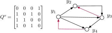
Figure 6: An example of the Boolean matrix and its digraph.

The lower triangular part of $Q^{o}$ specifies a block diagram (with unknown transfer functions) with only feedforward paths, and the upper triangular part adds feedback loops (marked in red in Fig. 6). The key is to use the small gain theorem to tune the added feedback transfer functions one by one to guarantee BIBO stability. The transfer matrix $Q(q)$ with structure $Q^{o}$ is created by generating random stable polynomials for nonzero entries in $A,B^{y}$ and $B^{u}$, where nonzero entries of $B^{y}$ are specified by $Q^{o}$, and then using (5). The last step is to tune the gain of each feedback transfer function, as specified by $Q^{o}_{U}$, using the small gain theorem sequentially. Here we will present an example to show the whole procedure. Suppose that the random structure for the 4-node network is specified by $Q^{o}$ and $P^{o}=[1\ 0\ 0\ 0]^{T}$ (the Boolean matrix of $P$), and the block diagram is shown in Fig. 7, where SISO transfer functions ($G_{1}(q),\dots,G_{8}(q)\in\mathcal{RH}_{\infty}$) are generated as aforementioned,

$$Q=\begin{bmatrix}0&0&0&\beta G_{7}(q)\\ G_{1}(q)&0&\alpha G_{6}(q)&0\\ G_{4}(q)&G_{2}(q)&0&0\\ G_{5}(q)&0&G_{3}(q)&0\end{bmatrix},P=\begin{bmatrix}G_{8}(q)\\ 0\\ 0\\ 0\end{bmatrix},$$ (47)

and $\alpha,\beta$ are positive real numbers that need to be tuned to guarantee stability, $\tilde{G}_{6}\triangleq\alpha G_{6}$, $\tilde{G}_{7}\triangleq\beta G_{7}$. We start with the inner loop (labeled as “loop 1” in Fig. 7) that is formed by the feedback item $\tilde{G}_{6}$, and applied the small gain theorem to the interconnected system shown in Fig. 8(a), which tells to choose $\alpha<1/(\|G_{2}\|_{\infty}\|G_{6}\|_{\infty})$. We then redraw Fig. 7 to remove the feedback path of $\tilde{G}_{6}$, as shown in Fig. 8(b), and the resultant whole block diagram turns to be Fig. 8(c), where $T_{1}=\frac{G_{1}+G_{4}G_{6}}{1-G_{2}\tilde{G}_{6}}$. Next we compute the lump-sum transfer function of all feedforward paths from $y_{1}$ to $y_{4}$ and present the following interconnected system in Fig. 8(d), where $T_{2}=(T_{1}G_{2}+G_{4})G_{3}+G_{5}$. By applying the small gain theorem, we choose $\beta<1/(\|T_{2}\|_{\infty}\|G_{7}\|_{\infty})$. As demonstrated by this example, the idea is to tune the feedback component sequentially, from inner loops (e.g., “loop 1” in Fig. 7) to outer loops (e.g., “loop 2”), using the small gain theorem to guarantee the internal stability.

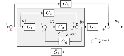
Figure 7: Block diagram of example (47) (neglecting inputs).

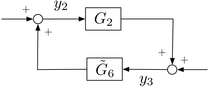
(a) lump-sum system

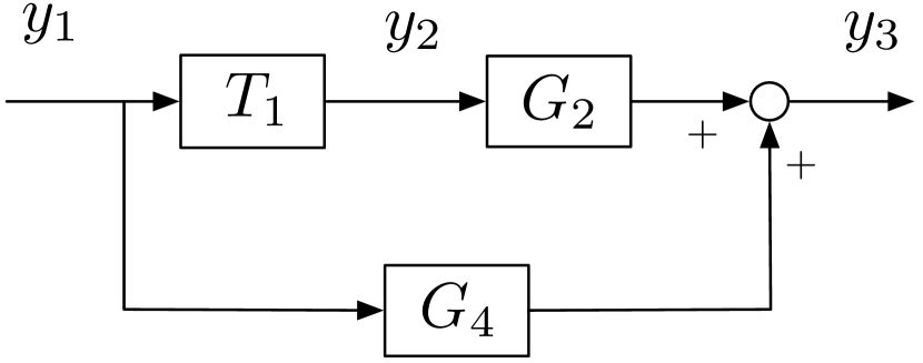
(b) intermediate subsystem

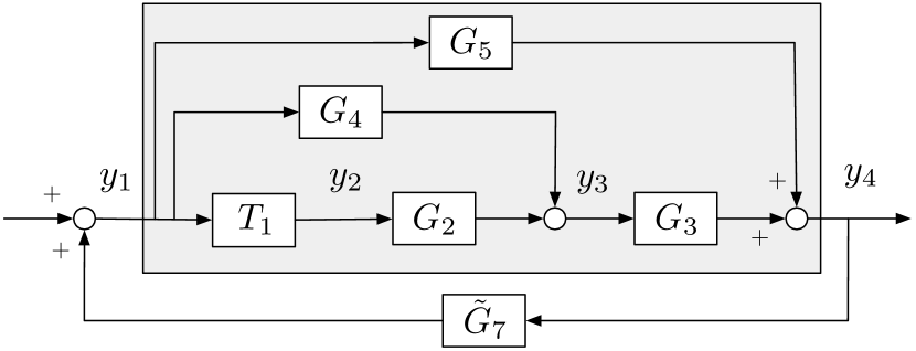
(c) intermediate system

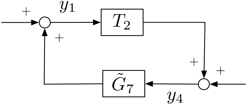
(d) lump-sum system

Figure 8: List of intermediate systems that assist the description of the whole procedure of stabilizing ARX networks in model generation.

This example uses the block diagrams to explain the procedure to apply the small gain theorem. In practice, the signal-flow graph is a better choice to represent complicated interconnections and helps to apply Mason’s gain formula to automate the computation of interconnected transfer functions. In our simulation, to ease the computation, up to networks of 20 nodes (see experiments for Fig. 3(b)), we add at most 3 feedback paths (since the path/loop finding is an NP problem and cost considerable time). Moreover, to simply computation, these feedback loops are either non-touching (no common nodes) or one is “contained” by the other (i.e., all the nodes in loop 1 appear in loop 2). Due to page limits, the general algorithms will be present in another paper to handle arbitrary feedback and feasibility of network stabilization. Before moving to the inference part, there is one implementation detail in MATLAB deserving to be shared. When you use control system toolbox in MATLAB and deal with many (e.g., $p>=10$) interconnections (connect in series or parallel, feedback), it may not be a good idea to compute the lump-sum transfer functions first, e.g., $T_{2}$ in Fig. 8(d), and then compute their infinity norms to apply the small gain theorem. The reason is that, even if at each step you guarantee the subsystems are correctly stabilized, the numeric errors in model interconnection using control system toolbox may lead to the resultant system being unstable (in theory it should be stable) and you are no longer able to continuing applying the small gain theorem. The solution used in our simulation is that, instead of computing the lump-sum transfer function, we compute the infinity norm of each transfer function (e.g., $T_{1},G_{2},G_{3},G_{4},G_{5}$ for $T_{2}$) first and then use Mason’s gain formula to compute an upper bound of $\|T_{2}\|_{\infty}$.

Appendix D Random generation of DSFs and benchmark

This section considers a Monte Carlo study of 50 runs of inference of random stable sparse networks (DSFs) with 40 nodes. In regard to the adjectives for DSFs, here are further explanations:

• random: the DSF model in each run is randomly chosen (both network topology and model parameters);

• stable: the DSF model is stable, i.e. all poles of $Q,P$ and $H$ have negative real parts, and all transmission zeros of $(I-Q)$ have negative real parts; (see [44, chap. 2.3])

• sparse: the number of arcs of the network is much less than that of a complete digraph.

The numerical example emulates the applications in practice, where the underlying systems evolves continuously in time and the proposed method uses parametric approaches to estimate network structures. Hence, we simulate the continuous-time DSF models and then sample the simulated signals with a chosen sampling frequency to acquire measurements for later network reconstruction. More details on the procedure is presented as below:

1. The DSF model will be simulated via its state space realization (both in continuous time). We randomly generate highly sparse stable $A$ matrices (of dimension $80\!\times\!80$) for state space models, and $B=[0,\dots,1,\dots,0]^{T}$, $C=[I_{40\times 40}\;0]$, $D=0$. The systems in replica are obtained by perturbing nonzero entries in the $A$ matrix.

2. The ground truth networks are calculated by the definition of DSF using $(A,B,C,D)$ (see [15]).

3. A step signal is chosen to be the input, and each state variable is perturbed by a Gaussian i.i.d. (i.e. process noises). The replica data is acquired by randomly perturbing non-zero elements in $A$ and performing simulation. The stochastic differential equation is numerically solved by using sim.m (choosing the Euler-Maruyama method) from system identification toolbox in MATLAB. The sampling frequency is chosen to be 40 times of the critical frequency of system aliasing (see [48]).

The setup of DSF models makes network inference particularly challenging. There may exist many loops due to feedback, whose sizes are fairly random. Moreover, we fill nonzero values in the position $A_{i,i+1}$ of the $A$-matrix to ensure each network will not degenerate into a family of separate small ones.

We apply the iterative reweighted $l_{1}$ method for group sparsity. The SBL and the sampling method fail mostly in the benchmark of random DSFs due to large modelling uncertainty using ARX parametrization. There is a “trade-off” between Prec and TPR when selecting regularization parameters $\lambda$. In theory, there could be an optimal value of $\lambda$ that gives large values of both Prec and TPR. However, in practice, the Prec is more critical in the sense that it has to be large enough to keep results useful. Otherwise, even if the TPR is large, the result will predicate too many wrong arcs to be useful in applications. As a rule implied from Fig. 9, in practice, we may choose a conservative value of $\lambda$ to make sure that we could have most predictions of arcs correctly; then, if more links need to be explored, we could decrease $\lambda$ to get more connections covered.

As known in biological data analysis, time series are usually of low sampling frequencies and have limited numbers of samples. To address the importance of these factors, we run the proposed method over a range of values, shown in Fig. 9. The sampling frequency is critical for applying discrete-time approaches for network inference (see [49]), which can be shown by Fig. 9. The simulation also tells that the length of time series that is at least four times larger than the number of unknown parameters could be a fair choice in practice for network reconstruction.

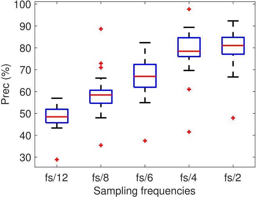
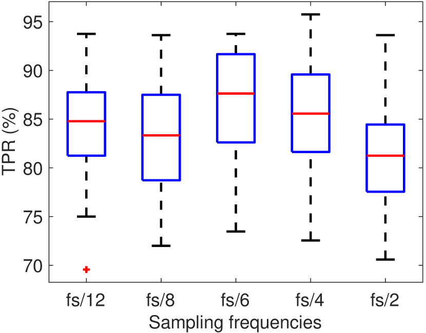
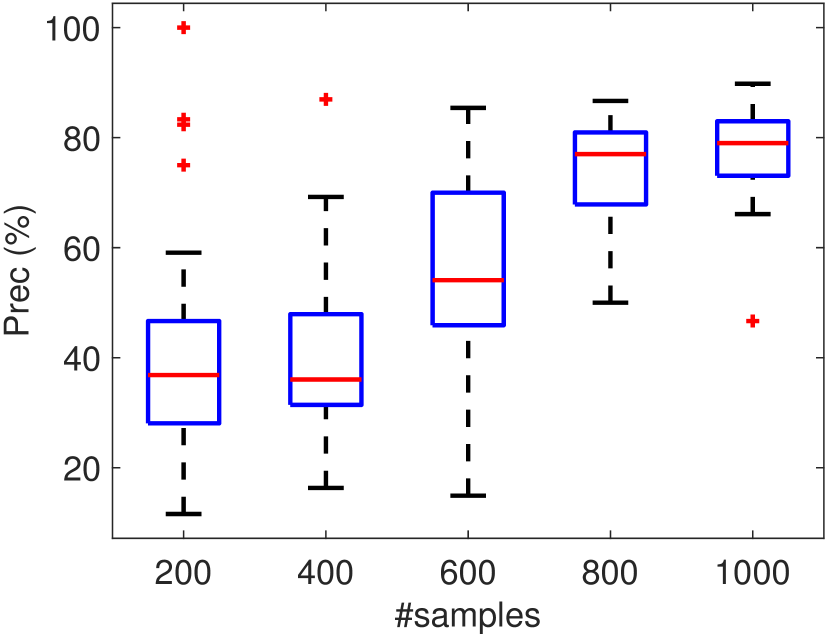
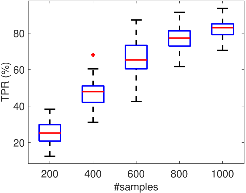
Figure 9: Performance of the proposed method on 50 random networks. The value of $\lambda$ is chosen by performing cross-validation on one network. The sampling frequency $f_{s}$ is the base value used in system simulations. The data used in reconstruction are sampled from the simulated signals. Here we use 2 replica datasets, e.g. “#samples = 800” implies each dataset has 400 samples.

Appendix E Supplementary benchmark results

The detailed result of the benchmark Fig. 3 in Section 6 is presented in Table 1. It summarises the means and standard deviations (SD) of performance indexes of the inference results, whose box plots shown in Figure 3.

Table 1: Summary of inference results for ARX dynamic networks. Each statistic is computed from inference results of 50 random models. The label “GIRL1” refers to the iterative reweighted $l_{1}$ method for group sparsity, “GSBL” refers to Sparse Bayesian Learning and “GSM” refers to sampling methods. In each test, all methods use the same data set, except that “GSM” only uses 100 points. In the simulation of multiple SNRs, the number of nodes is set to 10 (i.e. $p=10$); and in the case of multiple #nodes, the SNR is set to $10$ dB. The lambdas for “GIRL1” are set to $\lambda=0.1,0.1,0.01,0.001$ for $\text{SNR}=0,10,20,40\text{dB}$, respectively; and $\lambda=0.05,0.1,0.1,0.1$ for $p=5,10,15,20$.

(mean$\pm$SD)		SNRs (dB)
		0	10	20	40
Prec (%)	GIRL1	$98.96\pm 2.77$	$99.58\pm 1.73$	$97.94\pm 3.25$	$97.34\pm 4.25$
	GSBL	$89.92\pm 8.16$	$93.05\pm 6.95$	$93.31\pm 7.25$	$93.35\pm 6.64$
	GSMC	$99.89\pm 0.74$	$99.56\pm 1.53$	$99.65\pm 1.39$	$97.53\pm 3.80$
TPR (%)	GIRL1	$88.05\pm 9.51$	$83.06\pm 10.40$	$92.95\pm 7.24$	$95.52\pm 5.32$
	GSBL	$89.29\pm 8.25$	$89.14\pm 8.45$	$89.92\pm 8.81$	$88.79\pm 8.36$
	GSMC	$84.84\pm 10.37$	$87.80\pm 7.50$	$90.55\pm 7.49$	$94.01\pm 6.35$
(mean$\pm$SD)		#nodes
		5	10	15	20
Prec (%)	GIRL1	$100.00\pm 0.00$	$99.80\pm 1.41$	$99.45\pm 1.23$	$99.17\pm 1.74$
	GSBL	$94.47\pm 9.31$	$91.55\pm 6.87$	$93.66\pm 3.57$	$93.86\pm 4.45$
	GSMC	$100.00\pm 0.00$	$99.25\pm 2.07$	$99.01\pm 1.97$	$98.80\pm 3.02$
TPR (%)	GIRL1	$93.60\pm 10.25$	$86.23\pm 8.85$	$85.22\pm 9.85$	$86.82\pm 5.41$
	GSBL	$92.40\pm 11.35$	$89.05\pm 8.39$	$90.51\pm 8.59$	$90.89\pm 5.22$
	GSMC	$93.20\pm 10.39$	$88.68\pm 8.17$	$88.35\pm 8.78$	$89.67\pm 5.05$

One practical detail on implementing GSBL deserves our attention. A threshold in GSBL actually needs to be tuned to have better performance, which prunes the elements of $\boldsymbol{\gamma}$ (labeled as “pGamma” in Fig. 10) in the EM iterations. It determines whether the parameters that specific $\lambda$ corresponds to should be zero confidently. When dealing noisy data, a larger value of “pGamma” works better. The performance of different “pGamma” shows in Fig. 10, where the results with ill-selected “pGamma” comply with our intuition, that is a larger SNR gives obviously better performance.

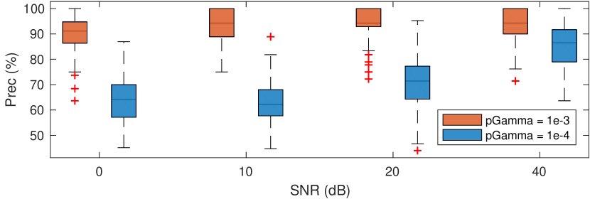
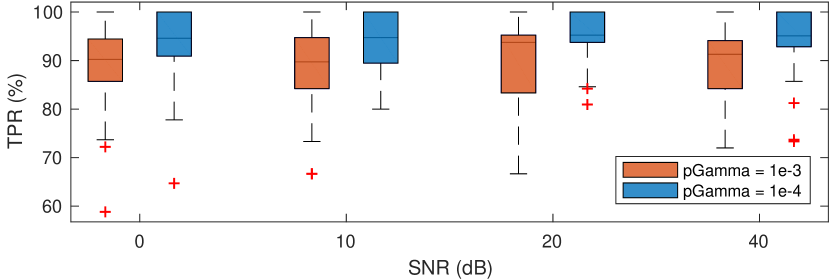
Figure 10: Performance of network inference using GSBL when setting different values to prune $\gamma$’s during the EM iterations.

Appendix F An illustrative example

This appendix presents a demo example to illustrate the whole idea/setup from Section 2- 4. In this demo project, we perform two experiments to collect data to infer the regulation relations between three variables $y_{1},y_{2}$ and $y_{3}$. Due to intrinsic difference of individuals or uncontrolled disturbance in experiments, the underlying system keeps the same mechanism (i.e. the regulation relations) but might differs in certain model parameters in two experiments, as shown in Fig. 11.

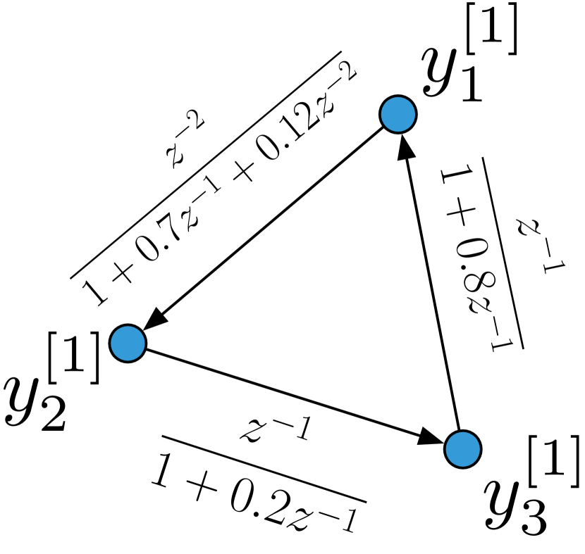
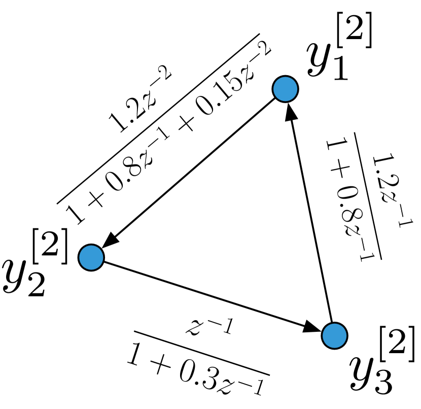
Figure 11: Models of the underlying system in two experiments, which share the same network structure but differ in parameters. Each variable is subject to a Gaussian white noise, which is omitted in the figure.

The network models in Fig. 11 can be expressed by DSFs,

$$\begin{array}[]{ll}y^{[1]}(t)&=Q^{[1]}(z)y^{[1]}(t)+H^{[1]}(z)e^{[1]}(t),\\ y^{[2]}(t)&=Q^{[2]}(z)y^{[2]}(t)+H^{[2]}(z)e^{[2]}(t),\end{array}$$ (48)

where

$$\begin{array}[]{ll}Q^{[1]}&=\begin{bmatrix}0&0&\frac{z^{-1}}{1+0.8z^{-1}}\\ \frac{z^{-2}}{1+0.7z^{-1}+0.12z^{-2}}&0&0\\ 0&\frac{z^{-1}}{1+0.2z^{-1}}&0\end{bmatrix}\\ Q^{[2]}&=\begin{bmatrix}0&0&\frac{1.2z^{-1}}{1+0.8z^{-1}}\\ \frac{1.2z^{-2}}{1+0.8z^{-1}+0.15z^{-2}}&0&0\\ 0&\frac{z^{-1}}{1+0.3z^{-1}}&0\end{bmatrix}\end{array}$$ (49)

and $H$ will be specified for convenience later on. Now consider $y_{2}$ as the example to show parametrization and the setup of multiple experiment data, where the object is to infer that $y_{1}$ regulates $y_{2}$ but $y_{3}$ does not. The whole network can then be reconstructed by independently repeating the same procedure on $y_{1}$ and $y_{3}$.

For simplicity, let this demo DSF be perfectly parametrized by ARX, and $H$ therefore is specified correspondingly,

$$\begin{array}[]{lll}&0.12y_{2}^{[1]}(t-2)+&0.7y_{2}^{[1]}(t-1)+y_{2}^{[1]}(t)=\\ &&y_{1}^{[1]}(t-2)+e_{2}^{[1]}(t),\\ &0.15y_{2}^{[2]}(t-2)+&0.8y_{2}^{[2]}(t-1)+y_{2}^{[2]}(t)=\\ &&1.2y_{1}^{[2]}(t-2)+e_{2}^{[2]}(t).\\ \end{array}$$ (50)

Assuming we set all orders of polynomials in ARX to be $2$, the regression model (11) is then be expressed as following

$$\begin{array}[]{lll}\hat{y}_{2}^{[1]}(t)&=&\begin{array}[t]{llllll}[&y_{1}^{[1]}(t-1)&y_{1}^{[1]}(t-2)&y_{2}^{[1]}(t-1)&y_{2}^{[1]}(t-2)&\\ &y_{3}^{[1]}(t-1)&y_{3}^{[1]}(t-2)&]\end{array}\\ &&\big{[}\begin{array}[]{cc:cc:cc}0&1&-0.7&-0.12&0&0\end{array}\big{]}^{T},\\ \hat{y}_{2}^{[2]}(t)&=&\begin{array}[t]{llllll}[&y_{1}^{[2]}(t-1)&y_{1}^{[2]}(t-2)&y_{2}^{[2]}(t-1)&y_{2}^{[2]}(t-2)&\\ &y_{3}^{[2]}(t-1)&y_{3}^{[2]}(t-2)&]\end{array}\\ &&\big{[}\begin{array}[]{cc:cc:cc}0&1.2&-0.8&-0.15&0&0\end{array}\big{]}^{T}.\\ \end{array}$$ (51)

Consider time points $t_{1},t_{2},t_{3}$ and set up the measurements from two experiments as (16w) in Section 4, yielding (52). Now we investigate the grouping patterns in the vector of parameters, which are marked in different colours in Fig. 12.

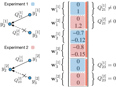
Figure 12: Illustration of parameter grouping and corresponding functions.

The parameters marked by blue boxes are ones of the model in Experiment 1 and ones marked by red boxes are of Experiment 2. Considering the consistency of network structures over experiments, we are obliged to guarantee the blue and red subgroups in one group indicated by orange boxes are both zero or nonzero. With the rearrangement of regressors as (16), the first and third groups determine which links exist in all experiment. To be specific, the arc from $y_{1}$ to $y_{2}$ should exist since both $Q_{21}^{[1]}$ and $Q_{21}^{[2]}$ are nonzero, while there is no arc from $y_{3}$ to $y_{2}$ since both $Q_{23}^{[1]}$ and $Q_{23}^{[2]}$ are identical to zero. Hence, in identification, we perform group sparsity with respect to groups indicated by orange boxes, which meanwhile also guarantees sparsity of network structures.

$$\begin{array}[]{lll}\left[\begin{array}[]{c}y_{2}^{[1]}(t_{1})\\ y_{2}^{[1]}(t_{2})\\ y_{2}^{[1]}(t_{3})\\ \hdashline y_{2}^{[2]}(t_{1})\\ y_{2}^{[2]}(t_{2})\\ y_{2}^{[2]}(t_{3})\end{array}\right]&=&\left[\begin{array}[]{cccc|cccc|cccc}y_{1}^{[1]}(t_{1}-1)&y_{1}^{[1]}(t_{1}-2)&0&0&y_{2}^{[1]}(t_{1}-1)&y_{2}^{[1]}(t_{1}-2)&0&0&y_{3}^{[1]}(t_{1}-1)&y_{3}^{[1]}(t_{1}-2)&0&0\\ y_{1}^{[1]}(t_{2}-1)&y_{1}^{[1]}(t_{2}-2)&0&0&y_{2}^{[1]}(t_{2}-1)&y_{2}^{[1]}(t_{2}-2)&0&0&y_{3}^{[1]}(t_{2}-1)&y_{3}^{[1]}(t_{2}-2)&0&0\\ y_{1}^{[1]}(t_{3}-1)&y_{1}^{[1]}(t_{3}-2)&0&0&y_{2}^{[1]}(t_{3}-1)&y_{2}^{[1]}(t_{3}-2)&0&0&y_{3}^{[1]}(t_{3}-1)&y_{3}^{[1]}(t_{3}-2)&0&0\\ \hdashline 0&0&y_{1}^{[2]}(t_{1}-1)&y_{1}^{[2]}(t_{1}-2)&0&0&y_{2}^{[2]}(t_{1}-1)&y_{2}^{[2]}(t_{1}-2)&0&0&y_{3}^{[2]}(t_{1}-1)&y_{3}^{[2]}(t_{1}-2)\\ 0&0&y_{1}^{[2]}(t_{2}-1)&y_{1}^{[2]}(t_{2}-2)&0&0&y_{2}^{[2]}(t_{2}-1)&y_{2}^{[2]}(t_{2}-2)&0&0&y_{3}^{[2]}(t_{2}-1)&y_{3}^{[2]}(t_{2}-2)\\ 0&0&y_{1}^{[2]}(t_{3}-1)&y_{1}^{[2]}(t_{3}-2)&0&0&y_{2}^{[2]}(t_{3}-1)&y_{2}^{[2]}(t_{3}-2)&0&0&y_{3}^{[2]}(t_{3}-1)&y_{3}^{[2]}(t_{3}-2)\end{array}\right]\\ &&\left[\begin{array}[]{c}0\\ 1\\ \hdashline 0\\ 1.2\\ \hline\cr-0.7\\ -0.12\\ \hdashline-0.8\\ -0.15\\ \hline\cr 0\\ 0\\ \hdashline 0\\ 0\end{array}\right]+\left[\begin{array}[]{c}e_{2}^{[1]}(t_{1})\\ e_{2}^{[1]}(t_{2})\\ e_{2}^{[1]}(t_{3})\\ \hdashline e_{2}^{[2]}(t_{1})\\ e_{2}^{[2]}(t_{2})\\ e_{2}^{[2]}(t_{3})\end{array}\right]\end{array}$$ (52)

References

- [1] Ziv Bar-Joseph, Anthony Gitter, and Itamar Simon. Studying and modelling dynamic biological processes using time-series gene expression data. Nature Reviews Genetics, 13(8):552–564, 2012.
- [2] Tatsuya Akutsu, Satoru Miyano, and Satoru Kuhara. Identification of genetic networks from a small number of gene expression patterns under the Boolean network model. In Pacific symposium on biocomputing, volume 4, pages 17–28. Citeseer, 1999.
- [3] Ilya Shmulevich, Edward R Dougherty, Seungchan Kim, and Wei Zhang. Probabilistic Boolean networks: a rule-based uncertainty model for gene regulatory networks. Bioinformatics, 18(2):261–274, 2002.
- [4] Kevin Murphy and Saira Mian. Modelling gene expression data using dynamic Bayesian networks. Technical report, 1999.
- [5] Judea Pearl. Probabilistic Reasoning in Intelligent Systems: Networks of Plausible Inference (Morgan Kaufmann Series in Representation and Reasoning). Morgan Kaufmann, 1988.
- [6] Kevin Patrick Murphy and Stuart Russell. Dynamic bayesian networks: representation, inference and learning. 2002.
- [7] Clive W J Granger. Investigating causal relations by econometric models and cross-spectral methods. Econometrica: Journal of the Econometric Society, pages 424–438, 1969.
- [8] Michael Eichler. Granger causality and path diagrams for multivariate time series. Journal of Econometrics, 137:334–353, 2007.
- [9] George Sugihara, Robert May, Hao Ye, Chih-hao Hsieh, Ethan Deyle, Michael Fogarty, and Stephan Munch. Detecting causality in complex ecosystems. science, 338(6106):496–500, 2012.
- [10] Cheng Hsiao. Autoregressive modeling and causal ordering of economic variables. Journal of Economic Dynamics and Control, 4:243–259, 1982.
- [11] Alessandro Chiuso and Gianluigi Pillonetto. A Bayesian approach to sparse dynamic network identification. Automatica, 48(8):1553–1565, 2012.
- [12] Eugene P van Someren, Lodewyk F A Wessels, and Marcel J T Reinders. Linear modeling of genetic networks from experimental data. In Ismb, pages 355–366, 2000.
- [13] Karl J Friston, Lee Harrison, and Will Penny. Dynamic causal modelling. Neuroimage, 19(4):1273–1302, 2003.
- [14] Matthew J Beal, Francesco Falciani, Zoubin Ghahramani, Claudia Rangel, and David L Wild. A Bayesian approach to reconstructing genetic regulatory networks with hidden factors. Bioinformatics, 21(3):349–356, 2005.
- [15] Jorge Goncalves and Sean Warnick. Necessary and Sufficient Conditions for Dynamical Structure Reconstruction of LTI Networks. Automatic Control, IEEE Transactions on, 53(7):1670–1674, 2008.
- [16] Paul M J Van den Hof, Arne Dankers, Peter S C Heuberger, and Xavier Bombois. Identification of dynamic models in complex networks with prediction error methods-Basic methods for consistent module estimates. Automatica, 49(10):2994–3006, 2013.
- [17] Harm H M Weerts, Arne G Dankers, and Paul M J Van den Hof. Identifiability in dynamic network identification. IFAC-PapersOnLine, 48(28):1409–1414, 2015.
- [18] Sean Warnick. Shared Hidden State and Network Representations of Interconnected Dynamical Systems. In 53rd Annual Allerton Conference on Communications, Control, and Computing, Monticello, IL, 2015.
- [19] D Hayden, Ye Yuan, and J Goncalves. Network reconstruction from intrinsic noise: Minimum-phase systems. In American Control Conference (ACC), 2014, pages 4391–4396, 2014.
- [20] David Hayden, Ye Yuan, and Jorge Goncalves. Network Reconstruction from Intrinsic Noise: Non-Minimum-Phase Systems. In Proceedings of the 19th IFAC World Congress, 2014.
- [21] David Hayden, Young Hwan Chang, Jorge Goncalves, and Claire J Tomlin. Sparse network identifiability via Compressed Sensing. Automatica, 68:9–17, 2016.
- [22] Donatello Materassi and Giacomo Innocenti. Topological identification in networks of dynamical systems. Automatic Control, IEEE Transactions on, 55(8):1860–1871, 2010.
- [23] Donatello Materassi and Murti V Salapaka. On the problem of reconstructing an unknown topology via locality properties of the Wiener filter. IEEE transactions on automatic control, 57(7):1765–1777, 2012.
- [24] Wei Pan, Ye Yuan, Lennart Ljung, Jorge Gon, and Guy-Bart Stan. Identifying biochemical reaction networks from heterogeneous datasets. In 2015 54th IEEE Conference on Decision and Control (CDC), pages 2525–2530. IEEE, 2015.
- [25] Feng He, Hairong Chen, Michael Probst-Kepper, Robert Geffers, Serge Eifes, Antonio del Sol, Klaus Schughart, An-Ping Zeng, and Rudi Balling. PLAU inferred from a correlation network is critical for suppressor function of regulatory T cells. Molecular Systems Biology, 8(1), nov 2012.
- [26] Zuogong Yue, Johan Thunberg, Wei Pan, Lennart Ljung, and Jorge Goncalves. Dynamic Network Reconstruction from Heterogeneous Datasets. arXiv:1612.01963, 2018.
- [27] Vasu Chetty and Sean Warnick. Network semantics of dynamical systems. In 2015 54th IEEE Conference on Decision and Control (CDC), pages 1557–1562. IEEE, 2015.
- [28] David Hayden, Ye Yuan, and Jorge Goncalves. Network Identifiability from Intrinsic Noise. IEEE Transactions on Automatic Control, PP(99):1, 2016.
- [29] L Ljung. System Identification: Theory for the User. Prentice-Hall information and system sciences series. Prentice Hall PTR, 1999.
- [30] Noah Simon and Robert Tibshirani. Standardization and the group lasso penalty. Statistica Sinica, 22(3):983, 2012.
- [31] Ming Yuan and Yi Lin. Model selection and estimation in regression with grouped variables. Journal of the Royal Statistical Society: Series B (Statistical Methodology), 68(1):49–67, 2006.
- [32] Emmanuel J Candes, Michael B Wakin, and Stephen P Boyd. Enhancing sparsity by reweighted l1 minimization. Journal of Fourier analysis and applications, 14(5-6):877–905, 2008.
- [33] Rick Chartrand and Wotao Yin. Iteratively reweighted algorithms for compressive sensing. In Acoustics, speech and signal processing, 2008. ICASSP 2008. IEEE international conference on, pages 3869–3872. IEEE, 2008.
- [34] Neal Parikh and Stephen Boyd. Proximal algorithms. Foundations and Trends in optimization, 1(3):123–231, 2013.
- [35] Stephen Boyd, Neal Parikh, Eric Chu, Borja Peleato, and Jonathan Eckstein. Distributed optimization and statistical learning via the alternating direction method of multipliers. Foundations and Trends in Machine Learning, 3(1):1–122, 2011.
- [36] Michael E Tipping. Sparse Bayesian learning and the relevance vector machine. The journal of machine learning research, 1:211–244, 2001.
- [37] David P Wipf and Bhaskar D Rao. Sparse Bayesian learning for basis selection. Signal Processing, IEEE Transactions on, 52(8):2153–2164, 2004.
- [38] David Wipf and Srikantan Nagarajan. Iterative reweighted l1 and l2 methods for finding sparse solutions. Selected Topics in Signal Processing, IEEE Journal of, 4(2):317–329, 2010.
- [39] David P Wipf and Bhaskar D Rao. An empirical Bayesian strategy for solving the simultaneous sparse approximation problem. Signal Processing, IEEE Transactions on, 55(7):3704–3716, 2007.
- [40] Lynn Kuo and Bani Mallick. Variable selection for regression models. Sankhya: The Indian Journal of Statistics, Series B, pages 65–81, 1998.
- [41] Jun S Liu. Monte Carlo strategies in scientific computing. Springer Science & Business Media, 2008.
- [42] James O Berger. Statistical Decision Theory and Bayesian Analysis (Springer Series in Statistics). Springer, 1993.
- [43] David A Van Dyk and Xiyun Jiao. Metropolis-Hastings within partially collapsed Gibbs samplers. Journal of Computational and Graphical Statistics, 24(2):301–327, 2015.
- [44] Zuogong Yue. Dynamic Network Reconstruction in Systems Biology: Methods and Algorithms. Ph.d. dissertation, University of Luxembourg, 2018.
- [45] Zuogong Yue, Johan Thunberg, and Jorge Goncalves. Network Stability, Realisation and Random Model Generation. In 2019 IEEE 58th Annual Conference on Decision and Control (CDC), pages 4539–4544, Nice, France, 2019.
- [46] Berkman Sahiner, Weijie Chen, Aria Pezeshk, and Nicholas Petrick. Comparison of two classifiers when the data sets are imbalanced: the power of the area under the precision-recall curve as the figure of merit versus the area under the ROC curve. In SPIE Medical Imaging, pages 101360G–101360G. International Society for Optics and Photonics, 2017.
- [47] Kemin Zhou and John Comstock Doyle. Essentials of robust control. Prentice Hall, Upper Saddle River, N.J., 1998.
- [48] Zuogong Yue, Johan Thunberg, and Jorge Goncalves. Inverse Problems for Matrix Exponential in System Identification: System Aliasing. In 2016 22nd Proceedings of International Symposium on Machematical Theory of Networks and Systems, 2016.
- [49] Zuogong Yue, Johan Thunberg, Lennart Ljung, Ye Yuan, and Jorge Goncalves. Systems Aliasing in Dynamic Network Reconstruction: Issues on Low Sampling Frequencies. arXiv 1605.08590, 2018.