Untangling galaxy components: full spectral bulge–disc decomposition

Abstract

To ascertain whether photometric decompositions of galaxies into bulges and disks are astrophysically meaningful, we have developed a new technique to decompose spectral data cubes into separate bulge and disk components, subject only to the constraint that they reproduce the conventional photometric decomposition. These decompositions allow us to study the kinematic and stellar population properties of the individual components and how they vary with position, in order to assess their plausibility as discrete elements, and to start to reconstruct their distinct formation histories. An initial application of this method to CALIFA integral field unit observations of three isolated S0 galaxies confirms that in regions where both bulge and disc contribute significantly to the flux they can be physically and robustly decomposed into a rotating dispersion-dominated bulge component, and a rotating low-dispersion disc component. Analysis of the resulting stellar populations shows that the bulges of these galaxies have a range of ages relative to their discs, indicating that a variety of processes are necessary to describe their evolution. This simple test case indicates the broad potential for extracting from spectral data cubes the full spectral data of a wide variety of individual galaxy components, and for using such decompositions to understand the interplay between these various structures, and hence how such systems formed.

1 Introduction

Almost since the study of galaxy evolution first began, bulge–disc decompositions have been used to try and understand the separate formation and evolution histories of each component. Originally, many galaxies were thought to comprise a central spheroidal bulge with a de Vaucouleurs law surface brightness profile (de Vaucouleurs, 1948) combined with a more extended exponential disc (Freeman, 1970). This division fits nicely with a dynamical picture in which part of the system consists of stars on largely random orbits, resulting in a spheroidal component with little net rotation, while the remainder is made up of stars in well-ordered rotation, producing a highly-flattened disc. Thus, bulge–disc decomposition offered a neat and convenient way of separating the different parts of a galaxy, and hence exploring the formation histories of these dynamically-distinct features. To this end, increasingly sophisticated software such as GALFIT (Peng et al., 2002), GIM2D (Simard, 1998) and BUDDA (de Souza et al., 2004) has been developed to formalise and automate the process of fitting such multiple components.

However, as the level of detail in observations has increased, evidence has appeared indicating that bulges and discs are not as simple and distinct as was first thought. With the high image resolution made possible with HST, it was found that many bulges display disc-like features such as spiral structure, inner discs and bars, and often follow shallower surface brightness profiles than originally thought, with Sérsic indices as low as the value of unity that is characteristic of an exponential disc (Sérsic, 1963; Andredakis & Sanders, 1994; Andredakis et al., 1995; Courteau et al., 1996; Carollo, 1998; MacArthur et al., 2004). In addition, work on the structure of bulges with boxier shapes has found that these components are actually thickened bars, an element that had originally been associated with galactic discs (Kuijken & Merrifield, 1995; Bureau & Freeman, 1999). Such developments have blurred the distinction between discs and bulges, and thus raised the question of whether the components obtained by decomposing a galaxy photometrically really represent individual stellar populations with distinct kinematics, or whether these decompositions are just a convenient way of parameterising galaxy light distributions.

The key to addressing this question is provided by spectra: since their absorption lines contain information on both stellar kinematics and populations, analysis of spectral data can in principle be used to test whether the individual bulge and disc components form coherent distinct entities in terms of their dynamics and stellar properties, and hence whether the decomposition makes any intrinsic physical sense.

Historically, spectral observations were obtained using long-slit spectrographs, which provided a one-dimensional cut through the light distribution of a galaxy. Johnston et al. (2012) developed a technique to decompose these profiles into bulge and disc components at each wavelength provided by the spectrograph, thus producing a direct measure of the amount of bulge and disc light as a function of wavelength; in other words, it extracted separate bulge and disc spectra, which would allow the stellar populations in these components to be compared. More recently, they have generalised the technique to analyse integral-field unit (IFU) data, which produce spectra right across the face of a galaxy, and hence generate a three-dimensional data cube comprising a spectrum at each location on the sky. By applying GALFITM (Häußler et al., 2013), a modified version of GALFIT, to an “image slice” through the data cube at each wavelength, it is possible to calculate the relative contributions of bulge and disc at that wavelength, and hence calculate a separate spectrum for each component as before, but now based on a more reliable two-dimensional image rather than just a one-dimensional cut (Johnston et al., in prep).

Although this approach has yielded new insights into the formation sequence of bulges and discs in S0 galaxies (Johnston et al., 2014), it is not well suited to addressing the question of the distinctness of the components. Because it reduces each component to a single spectrum, it loses most of the information relating to variations with position in the galaxy, which would tell us how homogeneous each component is. In addition, it throws away all the kinematic information in the spectra, even though some of the clearest defining features of bulges and discs are related to their distinct dynamical properties [see Cappellari 2016 for a review].

The presence of multiple galaxy components has also been previously explored through a purely kinematic approach. Bender (1990) found that the asymmetric shape of the line-of-sight velocity distribution along the major axis of discy elliptical galaxy NGC 4621 was best explained by the presence of two gaussians with different mean velocities and velocity dispersions, i.e. a bulge and a disc component. Subsequent studies such as Scorza & Bender (1995) used this effect to explore the kinematics of bulge and disc components for a wider sample of discy ellipticals. However, this approach is limited in terms of the spatial information, looking only at the behaviour along major axis of the galaxy, and does not provide information on the stellar populations of the components, which is also a key element in determining whether the components are truly distinct.

In this paper, we therefore attempt a new approach to decomposing galaxies into bulge and disc components, which retains both the kinematic and stellar population information, and allows freedom for the properties of each component to vary with position, subject only to the global constraint that the relative fluxes of bulge and disc component at each location match those produced by image decomposition. Thus these models, by construction, reproduce the bulge and disc components of the conventional image fitting technique, but also fit the full spectral data cube for the galaxy. By investigating the stellar kinematics and populations of the resulting fitted components, and how they vary with position, it will be possible to test whether the imposed image decomposition produces coherent underlying physical sub-systems.

2 Test data

To develop this approach, we need a few representative galaxy observations to test that the method is viable with the quality of data currently being obtained. There are an expanding number of IFU galaxy surveys from which such a test case could be drawn, including SAURON (de Zeeuw et al., 2002), ATLAS^3D (Cappellari et al., 2011), SAMI (Bryant et al., 2015) and MaNGA (Bundy et al., 2015). For this analysis, we have chosen to use data from the recently-completed Calar Alto Integral Field Area (CALIFA) survey (Sánchez et al., 2012), which obtained spatially-resolved spectroscopy of 600 nearby ($0.005\leq z\leq 0.03$) galaxies over a wide range of morphologies. We analyse an observation in the V1200 setup, which yielded spectra with a wavelength range of 3650–4840Å, and a spectral resolution of 2.3Å FWHM, corresponding to a velocity resolution of $\sim 80$ km s^-1 at the blue end and $\sim 60$ km s^-1 at the red end of the spectrum. A full description of the data can be be found in García-Benito et al. (2015).

From the CALIFA sample, we have selected three field S0 galaxies: NGC 528, NGC 7671 and NGC 6427. The SDSS colour images of these galaxies are shown in Figure 1, and the galaxies properties are summarised in Table 1. With their simple structure, all containing clear bulge and disc components and no visible dust, spiral structure or bar, they make good first test examples of such a bulge–disc decomposition method. Selecting this Hubble type and environment also allows us to compare and contrast the result with the previous analysis by Johnston et al. (2014) in their study of cluster S0s.

In order to fully determine the strengths and limitations of the method, we have chosen to explore the decomposition of one galaxy, NGC 528, in particular detail. At an inclination of $\sim 70$ degrees, it clearly displays both bulge and disc, while still ensuring that enough of any rotational motion is projected into the line of sight to be detected. It was also chosen for its brightness: it has a K-band absolute magnitude of $M_{K}\approx-24.36$ (Skrutskie et al., 2006); using eq.(2) of Cappellari (2013) this luminosity can be converted into a large stellar mass of $M_{\ast}\approx 1.5\times 10^{11}M_{\odot}$, ensuring that any kinematic structure will be well resolved with the CALIFA spectral resolution. The following sections will outline the method as applied to this galaxy.

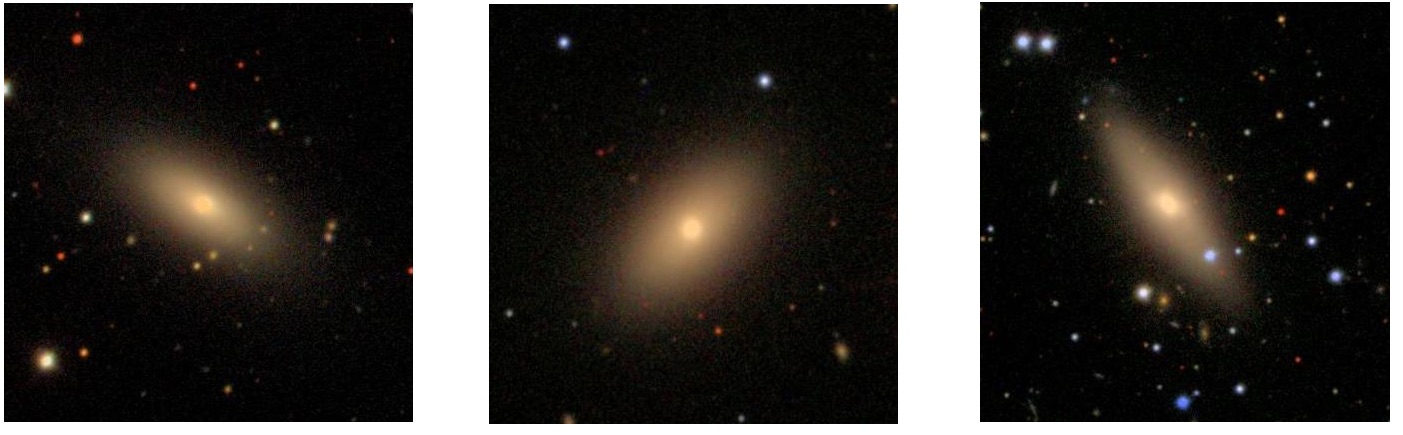
Figure 1: SDSS images of the three test galaxies over the CALIFA field of view; from left to right NGC 528, NGC 7671 and NGC 6427.

Galaxy	Kmag	$M/M_{\odot}$	I(∘)	Distance modulus
NGC 528	$-24.36$	$1.5\times 10^{11}$	70	$34.24$
NGC 7671	$-24.05$	$5.9\times 10^{10}$	75	$33.49$
NGC 6427	$-23.43$	$4.0\times 10^{10}$	90	$33.91$

Table 1: Absolute magnitude, stellar mass (converted from K-band magnitude using eq.(2) of Cappellari 2013), inclination and redshift distance modulus (Makarov et al., 2014) of galaxy sample.

3 Photometric bulge–disc decomposition

To perform the initial bulge–disc decomposition that tells us how much light to ascribe to each component at each point in the galaxy, we have first collapsed the data cube in the spectral direction to produce a fairly crude image of the galaxy at the appropriate spatial resolution. We applied GALFIT to this image to fit an exponential disc plus a spheroidal component with a Sérsic profile for which the index was left as a free parameter. We also left the position angle and flattening of each component as free parameters.

The specific point-spread function (PSF) for this observation is not part of the currently-released CALIFA data, so we modelled it as a narrow Moffat profile plus a broad low-intensity Gaussian as described in García-Benito et al. (2015), and varied its Moffat parameters to minimise the residuals between model and image data. The best fit was found to result from a PSF with a FWHM of $2.2\,{\rm arcsec}$, although the subsequent results do not depend sensitively on the exact value adopted.

The parameters of the derived best-fit galaxy models for the three sample galaxies are listed in Table 2, and an indication of the quality of the fit is provided in Figure 2, which shows data, model and residuals for NGC 528. The fit is generally very good, although the central asymmetric residual indicates that the galaxy seems to have a slightly off-centre nucleus, but this phenomenon has no effect on what follows. It is also interesting to note from Table 2 that this galaxy clearly favours an almost exponential bulge with a Sérsic index near unity, and is therefore an example of the non-classical bulge behaviour mentioned above.

	NGC 528		NGC 7671		NGC 6427
Parameter	Bulge	Disc	Bulge	Disc	Bulge	Disc
Half light radius/Scale length	$2.21^{\prime\prime}\pm 0.09^{\prime\prime}$	$9.17^{\prime\prime}\pm 0.11^{\prime\prime}$	$1.6^{\prime\prime}\pm 0.002$”	$8.68^{\prime\prime}\pm 0.05^{\prime\prime}$	$2.90^{\prime\prime}\pm 0.04^{\prime\prime}$	$9.88^{\prime\prime}\pm 0.11^{\prime\prime}$
Axis ratio	$0.78\pm 0.01$	$0.52\pm 0.01$	$0.93\pm 0.01$	$0.67\pm 0.002$	$0.797\pm 0.003$	$0.474\pm 0.003$
Sérsic Index	$1.07\pm 0.04$	$1.0$ (fixed)	0.99$\pm$0.04	1.0 (fixed)	0.93$\pm$0.03	1.0 (fixed)
Position Angle	$-89.8\pm 2.57$	$59.02\pm 0.15$	18.6$\pm$7.6	$-43.6\pm 0.3$	$64.8\pm 2.6$	$34.7\pm 0.3$
Flux Fraction	$0.275\pm 0.005$	$0.725\pm 0.005$	$0.277\pm 0.002$	$0.723\pm 0.002$	$0.320\pm 0.002$	$0.680\pm 0.002$

Table 2: Parameters of GALFIT photometric decomposition of collapsed data cube image of NGC 528, NGC 7671 and NGC 6427. Note the errors shown are statistical estimates directly from GALFIT, which underestimate the true uncertainties.

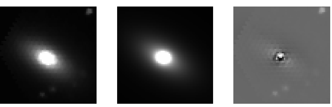
Figure 2: The collapsed CALIFA data cube for NGC 528, the GALFIT best fit model, and the residuals (galaxy minus model)

4 Spectroscopic bulge–disc decomposition

4.1 Method

In order to carry out the spectral decomposition, we need to fit bulge and disc components, weighted by their relative contribution at each spatial coordinate of the data cube, to the spectrum at that point. To this end, we have used the Python version of the penalised pixel-fitting code (Cappellari & Emsellem, 2004), updated as described in Cappellari (2017) which, from version 5.1, allows multiple components with different populations and kinematics to be fitted to spectra simultaneously (see Johnston et al. 2013).

For a given set of nonlinear parameters, pPXF solves a linear system for the weights of the spectral templates and additive polynomials, with the extra constraint that the weights of the spectral templates must be non-negative [eq. 3 in Cappellari & Emsellem (2004)]. This linear least-squares problem is solved by pPFX as a Bounded Variables Least Squares problem, with the specific BVLS method by Lawson & Hanson (1995).

Here we want to enforce an additional constraint to the problem: we require the template spectra describing the bulge component to contribute a prescribed fraction $f_{\rm bulge}$ of the total flux in the fitted spectrum

$$f_{\rm bulge}=\frac{\sum w_{\rm bulge}}{\sum w_{\rm bulge}+\sum w_{\rm disk}},$$ (1)

where $w_{\rm bulge}$ and $w_{\rm disk}$ are the weights assigned to the set of spectral templates used to fit the bulge and disk respectively.

This constraint could be implemented by using a generic quadratic programming algorithm to solve the linear least-squares sub-problem, while including equation (1) as an exact linear equality constraint. Instead, we chose a simpler route, which requires minimal changes to the pPXF algorithm. It consists of enforcing the equality constraint by adding the following single extra equation to the linear least-squares sub-problem

$$\frac{1}{\Delta}\left[(f_{\rm bulge}-1)\sum w_{\rm bulge}+f_{\rm bulge}\sum w_{\rm disk}\right]=0,$$ (2)

with the parameter $\Delta$ set to a very small number (e.g. $10^{-9}$), which specifies the relative accuracy at which this equation needs to be satisfied. When both the spectral templates and the galaxy spectrum are normalized to have a mean flux of order unity, the best fitting weights $w_{\rm bulge}$ and $w_{\rm disk}$ are generally smaller than unity and equation (2) is satisfied to numerical accuracy. This new option is activated by setting the keyword fraction from the Python pPXF version 5.2. Activating this option results in a negligible execution time penalty of the pPXF fit, when compared to an unconstrained fit.

4.2 Tests

The pPXF code requires that one specifies the base set of stellar populations from which the model is constructed. For this analysis, we have adopted the single stellar population templates of Vazdekis et al. (2010), providing high-resolution spectra for stellar populations with 7 different metallicities ranging from $-2.32$ to $0.22$ and 42 ages from $0.06\,{\rm~{}Gyr}$ to $17.8\,{\rm~{}Gyr}$, resulting in a total catalogue of 350 spectra. An age range that extends beyond the age of the Universe is required to account for uncertainties in the stellar population models. Linear combinations of this extensive library should provide a reasonable match to most stellar populations that we are likely to encounter, and offer at least an initial estimate of their ages and metallicities.

In general, the signal-to-noise ratio of the individual spectra in the data cube is not sufficient to fit simultaneously for kinematics and populations of multiple components. In order to determine at what signal-to-noise level this fit becomes possible, we have tested the method by decomposing a simulated galaxy spectrum composed of two stellar populations of different ages of 1 and 12 Gyrs, and with kinematics typical of a bulge and disc. To explore the full capabilities of the method we have looked at models with a galaxy bulge-to-total ratio of 0.3 and 0.5, and for each we vary the simulated signal-to-noise ratio from 10 to 35. To ensure the model is actually converging on the proper solution and does not simply return values close to the initial estimates, we have performed ten realisations at each signal-to-noise ratio, each time setting the initial kinematic estimates of both velocity and sigma to be a random value within 50 km s^-1 of the actual value. The best-fit kinematics and stellar populations at each signal-to-noise ratio are shown in Figure 3.

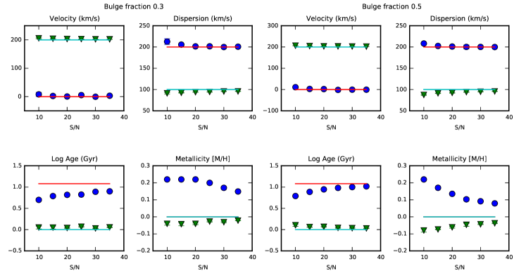
Figure 3: Best-fit kinematics and stellar populations for a simulated galaxy spectrum with bulge fractions of 0.3 and 0.5. Blue circles represent the median values of 10 realisations with varying initial estimates for the bulge, and green triangles represent the same for the disc. The error bars show the standard deviation of the 10 realisations. The solid line shows the actual values given to the components.

This test demonstrates the effectiveness of the method, showing that when both components contribute a significant amount to the flux their kinematics can be accurately determined and are not heavily dependant on the initial kinematic estimates. To retain as much spatial information as possible while avoiding significant biases, particularly in the derived metallicity, a signal-to-noise ratio of 25 was adopted for the decompostition. In order to obtain spectra of this quality from the CALIFA data cube, we co-added the data spatially using the Python version of the Voronoi binning code of Cappellari & Copin (2003).

We performed an additional test on the real CALIFA data cube, taking a sample of bins along the major axis of the galaxy and performing the decomposition for each bin over a grid of bulge and disk velocities, from $-400\,$ km s^-1 to $400\,$ km s^-1. pPXF uses a local non-linear optimization algorithm to fit the kinematics, starting from an initial guess for the parameters. However, with multiple kinematic components, the $\chi^{2}$ will generally present multiple local minima and there is no guarantee pPXF will converge to the global one. A simple brute-force way of finding the global minimum consists of sampling a regular grid of starting guesses with pPXF. By constraining the velocities of the fit to be within the pixel of the velocity grid, while letting the velocity dispersions vary freely, pPXF is forced to cover the full range of velocities, and we can therefore make sure we find the global rather than a possible local minimum for the $\chi^{2}$.

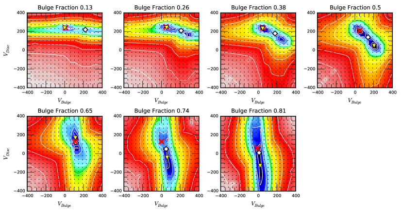
Figure 4: Chi-squared maps for a sample of bins along the major axis of the galaxy. One sigma contours are also plotted. Red crosses show the velocities found when pPXF is left free to vary, white diamonds show the velocity of a one component fit, and yellow triangles show the velocities for the lowest chi-squared grid pixels. When the yellow triangles and red crosses coincide, pPXF is effectively finding the global minimum from the estimated starting conditions.

The chi-squared map over this grid is shown in Figure 4 including one sigma contours, with the minimum chi-squared locations indicated by the yellow triangles. In order to evaluate how well pPXF finds this global minimum, the best-fit velocities found by pPXF when it is left free to vary are plotted as red crosses. As starting conditions for this free fit we took the velocity of a single component fit for the disc velocity, and the average velocity dispersion in the disc dominated region of the galaxy, here $144\,$ km s^-1 for the disc dispersion. For the bulge we estimated zero rotational velocity, and a velocity dispersion value of $200\,$ km s^-1.

This test gives us an insight both into how well pPXF finds the true best fit to the data when left free, and how accurately the kinematics of the components can really be determined overall for this quality of data.

As is to be expected, when a component dominates the flux pPXF effectively finds the best fit to the kinematics for this component when left free, and the velocity of this component is very well constrained, with the one-sigma contours covering a small range of velocities. However, the kinematics of the component with less flux are less likely to be found by pPXF and tend to show some degeneracy. This is especially apparent in bulge-dominated regions of the galaxy, with the one sigma contours stretching over a wide range of disc velocities. This is not surprising considering that in the very central regions of the galaxy there will be little difference in velocity between the two components, making it almost impossible to separate the LOSVDs effectively.

The tests also demonstrate that in the central regions of the galaxy, when pPXF is left free it does not always find the true chi-squared minima. Though the difference here is generally less than 3 sigma, for data of lower signal-to-noise and lower resolution this may not be the case. Therefore, we decided that to ensure that the true chi-squared minimum is found each time, when performing the decomposition on the full galaxy a simple 5x5 grid of velocities should be used for every voronoi bin.

Also important to note is that when both components contribute comparable fluxes two clear minima in chi-squared are visible, which have significantly lower chi-squared than the single component fit. This shows that the spectrum is better fit by two Gaussian components with different velocities and velocity dispersions, rather than one single Gaussian component. This is a first indication that two kinematically-distinct components do appear to be present in this galaxy.

It is worth noting that in conducting these tests we have built the machinery necessary to check the reliability of the decomposition process for any additional parameters, be it signal-to-noise ratio, initial kinematic estimates, component flux contribution etc. which will become useful when exploring new data and more complex systems.

4.3 NGC 528

In order to determine the kinematics of the bulge and disk implied by the assumed bulge-disk photometric decomposition, we have fitted each Voronoi bin with a kinematic model comprising two components with Gaussian line-of-sight velocity distributions. As demonstrated above (Section 4.2), in order to be certain that the true best fit to the spectra is being found, it is safest to force pPXF to cover a wide range of velocities for each component. For each Voronoi bin we therefore take the best fit to the spectrum across a 5x5 grid of velocities ranging from $-350\,$ km s^-1 to $350\,$ km s^-1. By constraining the resulting velocities of each fit to be within the pixel size of the grid, pPXF is forced to cover the whole velocity range and therefore find the true chi-squared minimum. The only additional constraint on the decomposition is that one component must reproduce the flux of the bulge derived in the photometric decomposition, while the other component must reproduce the disc flux. Both velocity dispersions and the stellar populations of the two components were left as free parameters. Since a change in kinematics can be slightly offset by altering the template spectra selected for the fit, it was deemed safest to continue to use the whole catalogue of 350 spectra to fit each component.

The resulting kinematic maps are presented in Figure 5. To avoid plotting noise and to give a clear indication where each component dominates, we have only reproduced the kinematic maps in regions where a component contributes at least 30% of the total flux. We found that below this level pPXF struggled to effectively distinguish the LOSVD of the lower flux component. The outer limit of the disc is determined by a minimum signal-to-noise threshold required for the Voronoi binning process, discarding pixels in the collapsed data-cube where the signal-to-noise ratio is too low.

It is apparent from this figure that this process decomposes the galaxy into remarkably coherent individual components, with a well-behaved symmetrically-rotating disc that has a low dispersion at all radii, and a symmetric high-dispersion rotating bulge with a dispersion profile that decreases in an orderly manner with radius. Note that the symmetric appearance of the kinematics is in no way imposed on the results: each spatial bin is decomposed independently, so the coherence of the map is a direct indicator of the consistency and reproducibility of the results, even down to the level where the component is only a 30% contributor to the total light.

The derived velocity dispersion of the bulge is high, but quite consistent with the central dispersion of $264\,$ km s^-1 found by Scodeggio et al. (1998), and the expected properties of such a massive galaxy (see Section 2). The mass of the galaxy is also reflected in the rotation speed of the disc, which, after correcting for inclination, implies a value of a little over $300\,$ km s^-1. Astrophysically, the rapid rotation of a low-Sérsic-index bulge is not surprising and agrees with multiple studies finding that these flatter bulges tend to display disc-like characteristics (see Kormendy & Kennicutt 2004 and references therein). The bulge rotation is also consistent with the finding that bulges and disks in fast rotator ETGs are best described by constant anisotropy (see Cappellari 2016 for a review).

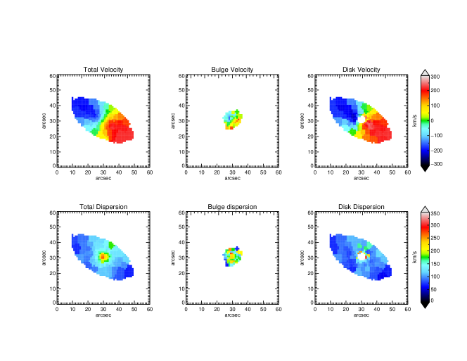
Figure 5: Kinematic maps for a one component fit (left) and two component fit (centre and right) for NGC 528

4.4 NGC 7671 and NGC 6427

Two other galaxies in this initial test, NGC 7671 and NGC 6427, were analysed in the same way. The galaxy magnitudes, masses and inclinations are shown in Table 1 and the parameters of the GALFIT photometric decomposition are shown in Table 2. Similar to NGC 528, both galaxies also possess low-Sérsic-index bulges, allowing us to gain further insight into these systems.

Figure 6 and Figure 7 show the resulting decomposed kinematic components. Again, the decompositions result in two very coherent components which match the photometric decomposition very well, and, as for NGC 528, both show cold rotating discs and hot rotating bulges. Comparing Figures 5, 6 and 7 there is a clear similarity in the kinematic components of these three galaxies as well as the photometric components. This suggests that not only do photometric decompositions represent individual stellar components, but the underlying kinematics of these components may potentially be deduced from their photometric parameters. Of course a much larger, more varied sample of galaxies will be required to determine if this relation holds in general.

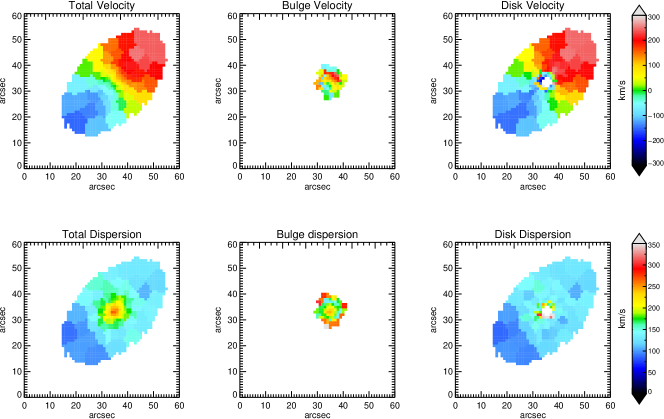
Figure 6: Kinematic maps for a one component fit (left) and two component fit (centre and right) for NGC 7671.

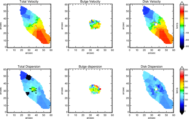
Figure 7: Kinematic maps for a one component fit (left) and two component fit (centre and right) for NGC 6427.

4.5 Stellar Populations

Since our fits also left the choice of stellar population completely free, as well as the weight assigned to each stellar population, they provide a measure of the age and metallicity of each component in each spatial bin, which yields further information on a galaxy’s past history. In particular, we can go beyond the analysis undertaken by Johnston et al. (2014) to look for spatial variations in the properties of the population within a single component. To illustrate the potential in such data, Figures 8, 9 and 10 show luminosity-weighted log age and metallicity of the single stellar population spectra selected by pPXF for the bulge and disc

$$<\textnormal{log age}>_{\rm component}=\frac{\sum(w_{\rm component}\times\textnormal{log age})}{\sum w_{\rm component}},$$ (3)

$$<[\textnormal{M/H}]>_{\rm component}=\frac{\sum(w_{\rm component}\times\textnormal{[M/H]})}{\sum w_{\rm component}},$$ (4)

where $w_{\rm component}$ are the weights assigned to the set of spectral templates used to fit each component.

Though the age and metellicity maps are more noisy than those of the kinematics, structure in the populations is clearly visible. The maps display an intriguing variation in populations across the components, with the three bulge components appearing younger, older, and of a similar age relative to their discs, while all three bulges are systematically more metal rich than their surrounding disc components.

It is interesting to compare this to ages and metallicities found for S0s in the Virgo cluster by Johnston et al. (2014), who showed that all the bulge components appeared to be younger than the discs. This suggests a difference in the evolutionary processes of cluster S0 galaxies and the field S0s studied here. Intriguingly, at larger radii there are also the first indications of structure in the metallicity and ages of the individual components that might allow us to go beyond a monolithic view of the formation of bulge and disc.

However, we must await the analysis of a larger sample to see how prevalent such features seen here may be and what implications they hold for the bigger picture of galaxy evolution. We also emphasise that this method thus far is primarily designed for decomposing the kinematics of the components, and exploring the most effective method for extracting accurate ages and metallicities is something that we intend look at in more detail in the future.

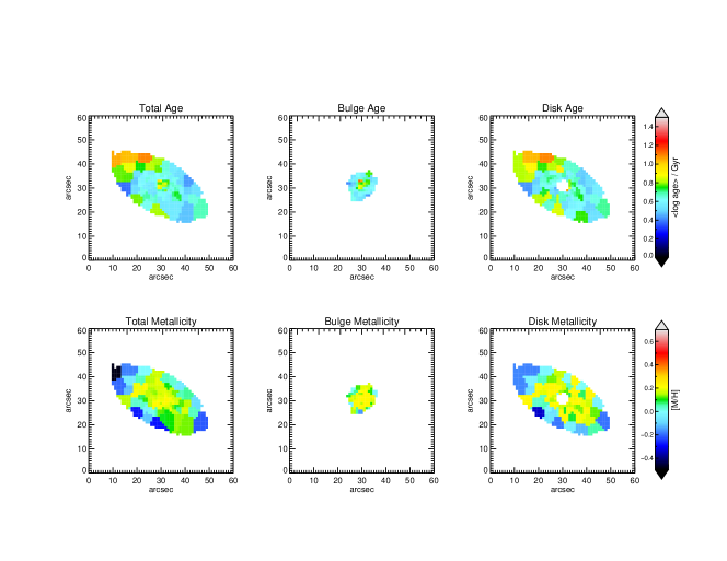
Figure 8: NGC 528: maps for the luminosity weighted ages and metallicities of the single stellar population spectra selected by pPXF for the one component kinematic model (left) and the two component kinematic model (centre and right). Bins where the flux of the component contributes less than 30% of the total flux are not included.

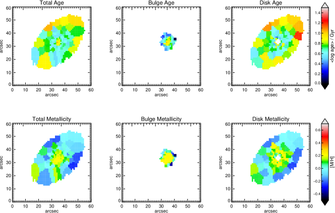
Figure 9: NGC 7671: maps for the luminosity weighted ages and metallicities of the single stellar population spectra selected by pPXF for the one component kinematic model (left) and the two component kinematic model (centre and right). Bins where the flux of the component contributes less than 30% of the total flux are not included.

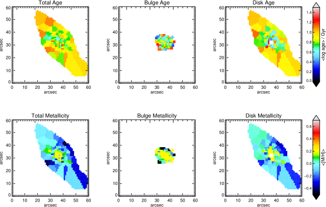
Figure 10: NGC 6427: maps for the luminosity weighted ages and metallicities of the single stellar population spectra selected by pPXF for the one component kinematic model (left) and the two component kinematic model (centre and right). Bins where the flux of the component contributes less than 30% of the total flux are not included.

5 Conclusions

In this paper, we have developed a method to find the kinematics and stellar populations of the bulge and disk components, when their relative surface brightness is constrained to be the one provided by a previous photometric decomposition.

An initial application of this technique to data cubes for three CALIFA S0 galaxies produces a remarkably coherent picture: these galaxies really can be separated into a cold rotating disc component and a hot rotating bulge component that match the expectations very well. Thus, at least for this test sample, the bulge and the disc do seem to represent plausible distinct components.

For this decomposition to be effective we have shown that the data ideally needs to be voronoi-binned to at least a signal-to-noise ratio of 25. To ensure that the true best fit to the data is found, it is best to run over a grid of component velocities for each voronoi bin. This allows the kinematics to be extracted effectively in this case down to a component flux contribution of  30% of the total flux; a level easily low enough to get detailed information on kinematics and stellar populations for each component.

In terms of the kinematics themselves, it appears that all three bulges are rotating; a finding which, given the low Sérsic-indices found for the bulges in the GALFIT photometric decomposition, agrees with previous literature on the disc-like characteristics often displayed by flatter bulges. With the ability to separate the kinematics of the bulge from those of the disc provided by this method, we can go beyond previous studies and look at the kinematics purely of the bulge component to see in what way they relate to the photometric parameters of the galaxy. Obtaining the kinematics of the components individually also provides useful raw material in modelling each component dynamically, presenting interesting opportunities to explore how the mass is distributed in the galaxy, and how this compares to the luminosity distribution.

We have also shown that there is information in the model stellar populations that produce the best fit. Previous studies into population gradients in S0 galaxies have produced a wide range of results, finding older bulge components than discs (Caldwell, 1983; Bothun & Gregg, 1990; Norris et al., 2006; González Delgado et al., 2015), similar ages in both components (Peletier & Balcells, 1996; Mehlert et al., 2003; Chamberlain et al., 2011), and older discs than bulges (Fisher et al., 1996; Bell & de Jong, 2000; Kuntschner, 2000; MacArthur et al., 2004). Studies specifically into S0 galaxies residing in clusters tend to find predominantly younger bulges than discs (Bedregal et al., 2011; Johnston et al., 2012), indicating that these S0s are most likely the evolutionary result of gas stripping from spiral galaxies, in which the “last gasp” of star formation occurred in their central regions, enhancing the bulge light.

The galaxies in this sample are found in the field and reflect this variation in populations gradients found in the studies mentioned above, suggesting that these galaxies, in contrast to S0s located in clusters, are not the result of one single evolution scenario.

In addition to these broad population differences, there are intriguing indications of structure within the metallicity and age maps of the decomposed bulges and discs, showing the potential of the method in revealing more detailed galaxy features. Not much should be inferred for such a small sample, but a systematic analysis of a larger number of galaxies could tell us a great deal about the channels through which these systems form and evolve. Fortunately, there is now no shortage of IFU observations of galaxies on which this technique could be used.

Finally, note that although we have concentrated on applying this method to the decomposition of galaxies into discs and bulges, it could equally well be applied to any other attempt to separate galaxies into components, such as multiple nuclei in giant ellipticals, cores and halos in cD galaxies, and even just line-of-sight blended images. It is also worth noting that any residuals to a fit, whether photometric or spectroscopic, are essentially just another component that can be treated in the same way, so one could, for example, look at the kinematics and stellar populations of spiral arms that might be left after the fitting of a smooth disc component to a spiral galaxy. As a general method, kinematic spectral decomposition constrained by photometric decomposition has many applications.

References

- Andredakis & Sanders (1994) Andredakis Y. C., Sanders R., 1994, MNRAS, pp 283–296
- Andredakis et al. (1995) Andredakis Y. C., Peletier R. F., Balcells M., 1995, MNRAS, 275, 874
- Bedregal et al. (2011) Bedregal A. G., Cardiel N., Aragón-Salamanca A., Merrifield M. R., 2011, MNRAS, 415, 2063
- Bell & de Jong (2000) Bell E. F., de Jong R. S., 2000, MNRAS, 312, 497
- Bender (1990) Bender R., 1990, A&A, 229, 441
- Bothun & Gregg (1990) Bothun G. D., Gregg M. D., 1990, ApJ, 350, 73
- Bryant et al. (2015) Bryant J. J., et al., 2015, MNRAS, 447, 2857
- Bundy et al. (2015) Bundy K., et al., 2015, ApJ, 798, 7
- Bureau & Freeman (1999) Bureau M., Freeman K. C., 1999, AJ, 118, 126
- Caldwell (1983) Caldwell N., 1983, ApJ, 268, 90
- Cappellari (2013) Cappellari M., 2013, ApJ, 778, L2
- Cappellari (2016) Cappellari M., 2016, ARA&A, 54, 597
- Cappellari (2017) Cappellari M., 2017, preprint (arXiv:1607.08538)
- Cappellari & Copin (2003) Cappellari M., Copin Y., 2003, MNRAS, 342, 345
- Cappellari & Emsellem (2004) Cappellari M., Emsellem E., 2004, Publications of the Astronomical Society of the Pacific, 116, 138
- Cappellari et al. (2011) Cappellari M., et al., 2011, MNRAS, 413, 813
- Carollo (1998) Carollo C., 1998, ApJ, 523, 566
- Chamberlain et al. (2011) Chamberlain L. C. P., Courteau S., McDonald M., Rose J. A., 2011, MNRAS, 412, 423
- Courteau et al. (1996) Courteau S., de Jong R. S., Broeils A. H., 1996, ApJ, 457
- Fisher et al. (1996) Fisher D., Franx M., Illingworth G., 1996, ApJ, 459, 110
- Freeman (1970) Freeman K. C., 1970, ApJ, 160, 811
- García-Benito et al. (2015) García-Benito R., et al., 2015, A&A, 576, A135
- González Delgado et al. (2015) González Delgado R. M., et al., 2015, A&A, 581, A103
- Häußler et al. (2013) Häußler B., et al., 2013, MNRAS, 430, 330
- Johnston et al. (2012) Johnston E. J., Aragón-Salamanca A., Merrifield M. R., Bedregal A. G., 2012, MNRAS, 422, 2590
- Johnston et al. (2013) Johnston E. J., Merrifield M. R., Aragón-Salamanca A., Cappellari M., 2013, MNRAS, 428, 1296
- Johnston et al. (2014) Johnston E. J., Aragón-Salamanca A., Merrifield M. R., 2014, MNRAS, 441, 333
- Kormendy & Kennicutt (2004) Kormendy J., Kennicutt R. C., 2004, ARA&A, 42, 603
- Kuijken & Merrifield (1995) Kuijken K., Merrifield M. R., 1995, ApJ, 443, L13
- Kuntschner (2000) Kuntschner H., 2000, MNRAS, 315, 184
- Lawson & Hanson (1995) Lawson C., Hanson R., 1995, Solving Least Squares Problems. Society for Industrial and Applied Mathematics
- MacArthur et al. (2004) MacArthur L. A., Courteau S., Bell E., Holtzman J. A., 2004, ApJS, 152, 175
- Makarov et al. (2014) Makarov D., Prugniel P., Terekhova N., Courtois H., Vauglin I., 2014, A&A, 570, A13
- Mehlert et al. (2003) Mehlert D., Thomas D., Saglia R. P., Bender R., Wegner G., 2003, A&A, 407, 423
- Norris et al. (2006) Norris M. A., Sharples R. M., Kuntschner H., 2006, MNRAS, 367, 815
- Peletier & Balcells (1996) Peletier R. F., Balcells M., 1996, AJ, 111, 2238
- Peng et al. (2002) Peng C. Y., Ho L. C., Impey C. D., Rix H.-W., 2002, AJ, 124, 266
- Sánchez et al. (2012) Sánchez S. F., et al., 2012, A&A, 538, A8
- Scodeggio et al. (1998) Scodeggio M., Giovanelli R., Haynes M. P., 1998, AJ, 116, 2728
- Scorza & Bender (1995) Scorza C., Bender R., 1995, A&A, 293
- Sérsic (1963) Sérsic J., 1963, Boletin de la Asociacion Argentina de Astronomia, 6
- Simard (1998) Simard L., 1998, in Albrecht R., Hook R. N., Bushouse H. A., eds, Astronomical Society of the Pacific Conference Series Vol. 145, Astronomical Data Analysis Software and Systems VII. p. 108
- Skrutskie et al. (2006) Skrutskie M. F., et al., 2006, AJ, 131, 1163
- Vazdekis et al. (2010) Vazdekis A., Sánchez-Blázquez P., Falcón-Barroso J., Cenarro A. J., Beasley M. A., Cardiel N., Gorgas J., Peletier R. F., 2010, MNRAS, 404, 1639
- de Souza et al. (2004) de Souza R. E., Gadotti D. A., dos Anjos S., 2004, ApJS, 153, 411
- de Vaucouleurs (1948) de Vaucouleurs G., 1948, Annales d’Astrophysique, 11
- de Zeeuw et al. (2002) de Zeeuw P. T., et al., 2002, MNRAS, 329, 513