Modular knowledge systems accelerate human migration in asymmetric random environments

Abstract

Migration is a key mechanism for expansion of communities. In spatially heterogeneous environments, rapidly gaining knowledge about the local environment is key to the evolutionary success of a migrating population. For historical human migration, environmental heterogeneity was naturally asymmetric in the north-south (NS) and east-west (EW) directions. We here consider the human migration process in the Americas, modeled as random, asymmetric, modularly correlated environments. Knowledge about the environments determines the fitness of each individual. We present a phase diagram for asymmetry of migration as a function of carrying capacity and fitness threshold. We find that the speed of migration is proportional to the inverse complement of the spatial environmental gradient, and in particular we find that north-south migration rates are lower than east-west migration rates when the environmental gradient is higher in the north-south direction. Communication of knowledge between individuals can help to spread beneficial knowledge within the population. The speed of migration increases when communication transmits pieces of knowledge that contribute in a modular way to the fitness of individuals. The results for the dependence of migration rate on asymmetry and modularity are consistent with existing archaeological observations. The results for asymmetry of genetic divergence are consistent with patterns of human gene flow.

1 Introduction

Interesting phenomena emerge in the population dynamics in heterogeneous environments. For example, experimental and theoretical studies have shown that spatial heterogeneity accelerates the emergence of drug resistance [1, 2] and solid tumor evolution in heterogeneous microenvironments [3]. On a larger scale, heterogeneity plays a central role in population biology of infectious diseases [4] and emerges in the development of large physics projects, such as ATLAS, CERN [5]. Finally, in heterogeneous environments, evolved networks are modular when there are local extinctions [6].

Populations experience heterogeneous environments during migration. Migration can occur in different dimensions: for example, cells undergo one-dimensional, two-dimensional, or three-dimensional migration [7]. In two-dimensional or three-dimensional migration, the environmental gradient can additionally be distinct in the different directions. For example, in the case of human migration, the north-south direction has a greater environmental gradient than does the east-west direction [8]. The heterogeneity is important in simulating human dispersal in the Americas [9]. In the east-west direction, food production spread from southwest Asia to Egypt and Europe at about $0.7$ miles per year around 5000 BC, while in the north-south direction, it spread northward in the American continent at about $0.2$ to $0.5$ miles per year around 2000 BC [8]. This spread is on the same order as the velocity of human migration, so we estimate that the human migration velocity in the east-west direction is about $2$ to $3$ times faster than in the north-south direction. Previous work has generated detailed migration paths using geographical data [10] as well as results that match existing archaeological evidences well after considering spatial and temporal variations [9]. We do not try to generate a detailed map of human migration in this paper. Instead, we use a general model to generate east-west north-south asymmetry and study the role of a modular knowledge system.

Knowledge of local environments, such as effective agricultural or animal husbandry techniques, was vital to the survival of these early migrants [8]. Evolutionary epistemology views the gaining of knowledge as an adaptive process with blind variation and selective retention [11]. Communication of knowledge between individuals is also an efficient means to spread this discovered, locally adapted knowledge [12]. Similarly, models of social learning theory stress the importance of social learning in the spread of innovations [13]. Here we model the adaptation of a population to the local environment using an evolutionary model with natural selection, mutation and communication. The knowledge of an individual determines his or her fitness. Evolutionary psychology and archeology posit that the human mind is modular [14], and that this modularity is shaped by evolution [15] and facilitates understanding of local environments [12]. Conjugate to this modularity must be dynamical exchange of corpora of knowledge between individuals [16, 17].

2 Methods

Table 1: Symbols used in this paper

Symbol	Meaning
$\chi$	Similarity between adjacent environments
$v$	Emigration velocity
$t$	Emigration time
$N$	Number of individuals in one environment
$N^{*}$	Carrying capacity of one environment
$N_{0}$	Initial population size of one environment
$f$	Fitness
$f^{*}$	Fitness threshold
$J$	Interaction matrix
$\Delta$	Connection matrix
$K$	Number of modules in a sequence
$l$	Module size
$\mu$	Mutational rate
$\nu$	Knowledge transfer rate
$d$	Genetic distance
$S$	A whole sequence
$s$	One locus in a sequence
$L$	Length of one sequence
$M$	Modularity

Table 1 shows the symbols in this paper. The observed emigration time and asymmetry of emigration time are critical in the determination of the values of these parameters. We consider migration in random, asymmetric, modularly correlated environments. We use $9\times 25$ correlated, random environments, where $25$ is the number of environments in the north-south direction at the same longitude [18], and $9$ is chosen so that $9/25$ is approximately the ratio of the east-west to north-south dimension of the Americas. See Fig. 1 for an illustration, where each square block corresponds to an environment.

Each individual a has a fitness $f_{\textbf{a}}$, as well as a sequence $S^{\textbf{a}}$ that is composed of $L$ loci, $s_{i}^{\textbf{a}}$, representing the knowledge of the individual. Fitness describes reproductive success and is proportional to the reproduction rate. For simplicity, we take $s_{i}^{\textbf{a}}=\pm 1$. We first consider a linear fitness landscape, later generalizing to an interacting landscape:

$$f[S] = 2L+H[S]$$

$$H[S] = \sum_{i}s_{i}J_{i}$$ (1)

where $J_{i}$ is a quenched, Gaussian random interaction parameter, with variance $\sqrt{2}$, and the offset $2L$ is chosen so that fitness is non-negative, since $H_{\min}$ is $-2L/\sqrt{\pi}$. For a given instance of the model, the interaction parameters $J_{i}$ are randomly chosen and then fixed for that instance of the model. When for each $i$ from $1$ to $L$, $s_{i}J_{i}>0$, the fitness reaches its highest value, and natural selection selects the sequence with the best configuration.

The fitness of the population is influenced by the environment, quantified by interaction parameters $J$, describing the interaction between knowledge element $i$ of the individuals and the environment (see also Eq. 1 above). The interaction parameters $J$ in two adjacent environments, $J$ and $J^{\prime}$, are correlated,

$$\langle J_{i}J^{\prime}_{i}\rangle/\langle J_{i}^{2}\rangle=\chi$$ (2)

where $\chi=\chi_{\rm{EW}}$ if the two have the same latitude, and $\chi=\chi_{\rm{NS}}$ if they have the same longitude. The smaller the $\chi$, the bigger the environmental gradient is. Here $0<\chi<1$, and $\chi_{\rm{NS}}<\chi_{\rm{EW}}$, since the gradient of environment in the north-south direction is more dramatic [8].

In each environment, we use a Markov process to describe the evolutionary dynamics, including replication with rate $f$, mutation with rate $\mu$ coming from discovering new knowledge through trial and error, and transfer of a corpus of knowledge of length $L/K$ with rate $\nu$. When individuals reproduce, they inherent the knowledge and genes from their parent without error. Both mutations and knowledge transfers are random, and they do not depend on the fitness of individuals. The relative rates of replication, mutation, and transfer are $f$, $\mu L$, and $\nu K$, respectively, so on average each individual makes $\mu L/f\approx\mu/2$ mutations, as $f\approx 2L$ at short times for which these populations evolve, and $\nu K/f\approx\nu K/(2L)$ knowledge transfers per lifetime of an individual. We set the information sequence length $L=100$. Discovery of new facts, represented by mutation, changes one site, or 1% of the knowledge of an individual, whereas knowledge transfer changes $1/K$ of the knowledge. Discovery of new facts should be rare, and in our simulation we set $\mu=0.5$, so that approximately one-quarter of the individuals attempt to make a discovery through trial and error during his or her lifetime. We consider $K=5$ corpora of knowledge. Transfer of one corpus, for example, could be one farmer attempting to communicate to another farmer how to grow a new crop in a new environment. Knowledge transfer must be rare, so we set $\nu=6$, so that roughly $\nu K/(2L)\approx 1/7$ of the individuals attempt a knowledge transfer process during his or her lifetime. We additionally consider various values of $\nu$ in this work to investigate the coupling of $\nu$ to modularity. Selection is based on the fitness of the knowledge and it determines the the utility of theses mutation and knowledge transfer events.

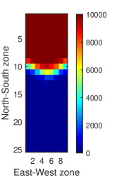
Figure 1: Population distribution half way through the migration. Color indicates density of the population in each environment. The maximum capacity of each environments is $N^{*}=10000$. Initially there are $1000$ individuals in the top center environment $(1,5)$, and no individuals in other environments. Here $\chi_{\text{EW}}=0.8$, $\chi_{\text{NS}}=0.4$, $f^{*}-2L=0.3L$, $L=100$, $\mu=0.5$, $\nu=6$, and $K=5$. Density was averaged over $24$ runs.

This dynamics of migration is described by a Markov process, whose master equation is detailed in the Appendix. Initially, one of the environments with the highest latitude is occupied by $1000$ individuals with random sequences, as Native Americans are believed to have entered the Americas through Alaska in the north. Since the population migrates from north down to south, we only allow migration to the east, west, and south. In each environment, the population evolves according to the Markov dynamics.

The qualitative behavior of the migration depends on the carrying capacity, $N^{*}$, and the fitness threshold, $f^{*}$. The carrying capacity is defined as the maximum population load of an environment [19]. After the population size reaches $N^{*}$, we randomly kill an individual every time another individual reproduces, as described in detail in Eq. 12. As a result, the total number of individuals does not exceed $N^{*}$. The initial colonization of the Americas occurred before the Common Era, for which there are no reliable population data.

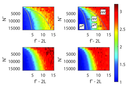
Figure 2: Asymmetry in emigration times $t_{\text{NS}}/t_{\text{EW}}$ for different $N^{*}$ and $f^{*}$. Upper left, phase diagram of the linear model, Eq. 1. Upper right, phase diagram of the quadratic model, Eq. 3, with $M=1$. Lower left, phase diagram of the quadratic model, with $M=1/2$. Lower right, phase diagram of the quadratic model, with $M=0$. Other parameters are as in Fig. 1. The color indicates the asymmetry in emigration times: $t_{\rm NS}/t_{\rm EW}$. There are three phases, with the boundaries denoted by the two curves. The steady-state fitness dynamics, $f(t)$ vs $t$, of the right phase and the left phase are shown in inset. The fitness dynamics of the middle phase in the north-south direction follows that of the upper inset, and in the east-west direction follows that of the lower inset. The phase boundaries are given approximately by equating the times in Eq. 4 for the north-south (left) or east-west (right) migration directions for linear model and $M=1$ quadratic model. The model for human migration has $N^{*}=10000$ and $f^{*}-2L=30$.

It is estimated that there were seven million people in the Americas at the start of the Common Era [20], corresponding to $7000000/(25\times 9)=31111$ individuals in each environment. We choose the carrying capacity to be $N^{*}=10000$, less than $31111$, reflecting that the population size was smaller the earlier time of initial population expansion. We show the results for various $N^{*}$ in Fig. 2. We introduce the fitness threshold, $f^{*}$, because individuals need to be well prepared before emigrating to the next environment. For example, young male ground squirrels appear to disperse after attaining a threshold body mass [21], and dispersing males tend to have greater fat percentage for their bodies [21]. The increased body mass and fat percentage are thresholds required for migration. Similarly, naked mole-rats migrate more frequently after body mass reaches a certain value [22]. It is possible that some individuals try to emigrate without reaching the fitness threshold when the local population size reach environmental capacity. However, they are not fit enough to colonize the new environment. Thus, we employ a fitness threshold in our approach, and allow no emigration before the average fitness value reaches $f^{*}$. When the population size reaches $N^{*}$ and the average fitness reaches $f^{*}$ in an environment, we move $N_{0}=1000$ randomly chosen individuals to one of the unoccupied adjacent environments. Fitter individuals may be more likely to migrate since they are physically better prepared to migrate, while on the other hand less fit individuals may have more desire to migrate since they do not live well in the current environment. We randomly choose individuals to migrate because of this ambiguous relationship between fitness and migration. If we move fitter individuals instead of randomly chosen individuals, the initial fitness of the individuals in the new environment will be higher. Thus, effectively the $\chi$ would be higher. The time required for a population to emigrate from an environment is denoted by the emigration time, $t$, and the emigration velocity $v$ is defined as $v=1/t$. The emigration time of an environment is the time from the arrival of the first individuals to the departure of the first individuals.

To compare our results with current human genetic data, we assign to each individual another sequence $S^{\prime}$, also composed of $L$ loci, and each locus can take values $\pm 1$. These sites correspond to automosal microsatellite marker genotype data [23], which we will compare with later in this paper. The traits of the genetic data are neutral in our model. That is, the values of the loci in the sequence $S^{\prime}$ have no effect on the fitness. The genetic sequence mutates at a rate $\mu^{\prime}$. When an individual reproduces, both the knowledge sequence and the genetic sequence reproduce.

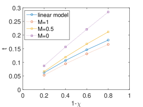
Figure 3: Emigration time versus $1-\chi$ for the linear model and the quadratic model with various modularities. Here $\chi_{\rm EW}=\chi_{\rm NS}=\chi$, and other parameters are as in Fig. 1.

We set the time scale in our simulation by the observation that Native Americans spent about $10000$ years to migrate from the north tip of the American continent to the south tip [24], experiencing about $25$ climate zones [18], so migration to a new environment occurred roughly every $400$ years, i.e. roughly every $20$ generations. In our simulation, we define a generation as the time period during which on average, each individual is replaced by another individual. We find that the population migrates approximately once per $20$ generations when $\chi_{\text{EW}}=0.8$, $\chi_{\text{NS}}=0.4$, and $f^{*}-2L=0.3L$. One can estimate how many generations it takes to migrate to the next environment. The rate of change of fitness at short time roughly follows [25],

$$df/dt=2L$$ (3)

Since $\Delta f=0.6\times(f^{*}-2L)=0.18\times 2L$ for migration from the north or $\Delta f=0.2\times(f^{*}-2L)=0.06\times 2L$ for migrating from the east or west, the emigration time is $0.18$ or $0.06$ depending on the origin of migration, and this is consistent with Fig. 3. We use $\Delta t=0.1$ as a rough estimate for emigration time. To convert this time in our simulation to number of human replications, we consider that one replication takes around $dt=1/f=1/2L$ time, so one emigration takes $\Delta t/dt=20$ generations. To compare the genetic data with current human data, we allow all environments to evolve for another $10000$ years after all environments are occupied, without migration between environments. We assume no gene flows between these environments, as previous work [26] assumes that the asymmetry in the genetic distance originates from the asymmetry of gene flows in different directions. Here we investigate another possible origin of the asymmetry of genetic distance, that is, the asymmetry already exists when the population colonized the Americas. It is quite possible that both mechanisms help to create this asymmetry, but in order to show that the initial colonizing process itself could generate this asymmetry, we suppress the possibly asymmetric genetic flows.

3 Results

In Fig. 1 we show a snapshot of population distribution, approximately half way through the migration. Migration sweeps south and spreads both to the east and west. Migration forms a tilted front, with slope magnitude equal to $v_{\text{NS}}/v_{\text{EW}}=0.35$, indicating the velocities of migration in different directions are different.

In Fig. 2 we show the three possible phases for different carrying capacity, $N^{*}$, and fitness threshold, $f^{*}$. Different phases correspond to whether the migration is limited by the fitness threshold or the population size threshold. In the left phase, the population is limited by the population size threshold, and there is no east-west north-south asymmetry. In addition, as the population migrates, the maximum fitness value increases since the population is allowed to evolve further after reaching the fitness threshold, as shown in the left inset of the upper right figure. In the middle phase, the migration in the east-west direction is limited by population size threshold while the migration in the north-south direction is limited by the fitness threshold. The maximum fitness value increase as the population migrates in the east-west direction, but in the north-south direction, the maximum fitness value is $f^{*}$. The degree of the east-west north-south asymmetry increases in this phase from the boundary with the left phase to the boundary with the right phase. In the right phase, migrations in both directions are limited by the fitness threshold, and the maximum fitness value remains the same as the population migrates. The east-west north-south asymmetry is approximately unchanged in this phase. The boundaries of these phases are determined by noting the times to reach the carrying capacity and the fitness threshold:

$$t_{N^{*}} = \frac{\ln(N^{*}/N_{0})}{2L}$$

$$t_{f} = \frac{(f^{*}-2L)(1-\chi)}{2L}$$ (4)

where $N_{0}$ is the initial population of one environment. Here we have used that the evolution of the fitness in one generation is small compared to the offset $2L$, and that the evolution within one environment at steady state is from $\chi(f^{*}-2L)+2L$ to $f^{*}$ in the rightmost phase. The left phase boundary in Fig. 2 is given by the condition $t_{N^{*}}=t_{f}$ in the north-south direction, and the right phase boundary is given by $t_{N^{*}}=t_{f}$ in the east-west direction. We note that our current choice of parameters is deep in the right phase, indicating that the east-west north-south asymmetry is robust to the change of $f^{*}$ or the ratio $N^{*}/N_{0}$.

We determine quantitatively how the environmental gradient influences the velocity of migration. In Fig. 3 we show the emigration time versus $1-\chi$, the change between adjacent environments. It is interesting that the emigration time is approximately proportional to $1-\chi$. This occurs because in our simulation for these parameters, the population reaches $N^{*}$ earlier than $f^{*}$, so the emigration time is the time required to reach $f^{*}$. For our model, $f^{*}-2L=0.3L$, while $\max(f-2L)\approx 2L$, so $f^{*}$ is still far from optimal, and the fitness increases linearly with time in the regime we are discussing. So $t=\Delta f/v_{f}=(1-\chi)f^{*}/v_{f}$, where $v_{f}$ is a constant for a fixed modularity. So $t\propto 1-\chi$, and we quantify the ratio of velocity in the two different directions as

$$\frac{v_{\text{EW}}(M)}{v_{\text{NS}}(M)}=\frac{1/t_{\text{EW}}(M)}{1/t_{\text{NS}}(M)}=\frac{1-\chi_{\text{NS}}}{1-\chi_{\text{EW}}}$$ (5)

In the linear model, it is quite easy to evolve the optimal pieces of knowledge, while in reality, finding the best knowledge is difficult at the individual level. We now show that these results are robust to considering an interacting model, while also demonstrating the significance of the modularity order parameter in the interacting model. As finding optimal knowledge for a local environment is difficult, the fitness landscape is rugged [27], and we use a spin glass to represent the fitness:

$$f[S] = 2L+H[S]$$

$$H[S] = \sum_{ij}s_{i}s_{j}J_{ij}\Delta_{ij}$$ (6)

where $J_{ij}$ is a Gaussian random matrix, with variance $1/C$. The offset value $2L$ is chosen by Wigner’s semicircle law [28] so that the minimum eigenvalue of $f$ is non-negative. The entries in the matrix $\Delta$ are zero or one, with probability $C/L$ per entry, so that the average number of connections per row is $C$. The optimization of this fitness model is hard when $L$ is large, and here we give a simple example to show why. Consider a case when $J_{ij}>0$, $J_{ik}>0$ and $J_{jk}<0$ given $i$, $j$ and $k$. To make $J_{ij}s_{i}s_{j}$ positive and fitness value larger, $s_{i}$ and $s_{j}$ must have the same sign. Similarly, to make $J_{ik}s_{i}s_{k}$ and $J_{jk}s_{j}s_{k}$ positive, we need $s_{k}$ to have the same sign with $s_{i}$, and $s_{k}$ to have different sign with $s_{j}$. This indicates that $s_{i}$ and $s_{j}$ have different signs, contradicting that $s_{i}$ and $s_{j}$ having the same sign. This phenomena is called frustration in physics [29], making the fitness hard to optimize. Let us exemplify this using an example from the human knowledge system. Humans developed three pieces of knowledge: the knowledge of toxicity of mushrooms, the knowledge of red food, and the knowledge of apples. The interaction between the first two pieces of knowledge implies that red food is bad and undesirable, while the later two pieces of knowledge implies something on the contrary. As a result the human knowledge system can be difficult to optimize. We will discuss how modularity helps to reduce this frustration and thus makes it easier to optimize the fitness in section 4.

We introduce modularity by an excess of interactions in $\Delta$ along the $l\times l$ block diagonals of the $L\times L$ connection matrix. There are $K$ of these block diagonals, and $K=L/l$. Thus, the probability of a connection is $C_{0}/L$ when $\lfloor i/l\rfloor\neq\lfloor j/l\rfloor$ and $C_{1}/L$ when $\lfloor i/l\rfloor=\lfloor j/l\rfloor$. The number of connections is $C=C_{0}+(C_{1}-C_{0})/K$, and modularity is defined by $M=(C_{1}-C_{0})/(KC)$. In Fig. 4 we illustrate three $20\times 20$ matrices with modularities $1$, $0.5$ and $0$ and $C=9$.

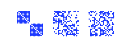
Figure 4: Illustration of $L=20$ connection matrices with different modularities. Left, a completely modular connection matrix, $M=1$. Middle, a moderately modular connection matrix, $M=0.5$. Right, a non-modular connection matrix, $M=0$.

Modularity, coupled with knowledge transfer, accelerates the evolution of a population in a new environment [25]. We now check how modularity and knowledge transfer influence the velocity of migration. For different $M$ and $\nu$, the results are shown in Fig. 5. For small $M$, a larger $\nu$ implies a smaller migrating velocity, indicating that the transfer of (non-useful) knowledge slows down evolution. As modularity increases, the migration velocity at larger $\nu$ catches up with that of smaller $\nu$. At $M=1$, in the range of $\nu$ shown, the faster the population migrates faster for larger $\nu$.

We fit the curve of $v_{\rm NS}$-$M$ for $\nu\leqslant 4$ in Fig. 5 with linear regression, observing $R^{2}\geqslant 0.95$, except for $\nu=0$, which has a zero slope and larger noise. We also fit the data for $\nu=1$ and $\nu=3$, not shown in Fig. 5. We show $dv_{\text{NS}}/dM$ versus modularity for different $\nu$ in the inset to Fig. 5. For $\nu\leqslant 4$, the slope is proportional to $\nu$. So, $dv_{\text{NS}}/dM=\alpha_{\text{NS}}\nu$, and after integration we have,

$$v_{\text{NS}}=\alpha_{\text{NS}}\nu M+v_{\text{NS}}^{0}(\nu)$$ (7)

where $v_{\text{NS}}^{0}(\nu)$ is determined by the evolutionary load of knowledge transfer. Linearity originates from perturbation of knowledge transfer when $\nu$ is small. Note that for $\nu=6$, the value used in most part of this paper, the linear relationship no longer holds, indicating that $\nu=6$ is large enough to break the linearity.

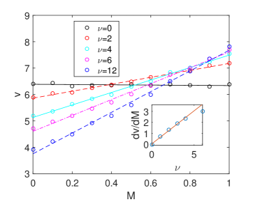
Figure 5: North-south Emigration velocity versus modularity for different $\nu$. The lines are linear fit of the data of the corresponding horizontal gene transfer rate. The inset shows $dv_{\rm NS}/dM$ versus $\nu$. The dots are data points and the line is a linear fit to the data. Other parameters are as in Fig. 1.

From our model, we make a prediction by calculating genetic distances between populations in different environments, using the genetic sequence $S^{\prime}$. For each pair of environments, we calculate the fixation index $F_{\text{ST}}$ between them using Eq. 5.12 from [30]:

$$F_{\text{ST}}=\frac{\sum_{i=1}^{L}\left[\frac{1}{2}\sum_{j=1}^{2}(p_{ij}-p_{ij}^{\prime})^{2}-\frac{1}{2(2n-1)}\left(2-\sum_{j=1}^{2}(p_{ij}^{2}+p_{ij}^{\prime 2})\right)\right]}{\sum_{i=1}^{L}(1-\sum_{j=1}^{2}p_{ij}p_{ij}^{\prime})}$$ (8)

where $p_{i1}$ is the probability of the value of locus $i$ being $+1$, and $p_{i2}$ is the probability of the value of locus $i$ being $-1$ in the first environment. $p_{ij}^{\prime}$ is the corresponding probability in the other environment. Here $n$ is the sample size drawn from the population to estimate $F_{\text{ST}}$, and in our case $n=18$, in accordance with the average sample size used in [26].

The east-west distance between environments $(x_{1},y_{1})$ and $(x_{2},y_{2})$ is $d_{\text{EW}}=|x_{1}-x_{2}|$, and the north-south distance is $d_{\text{NS}}=|y_{1}-y_{2}|$. We also calculated heterozygosities of the population of environment a, defined as

$$\text{het}_{a}=1-\frac{1}{L}\sum_{i=1}^{L}\sum_{j=1}^{2}p_{ij}^{2}$$ (9)

where $p_{i1}$ and $p_{i2}$ have the same meanings as those in Eq. 8. Each fixation index $F_{\text{ST}}$ was regressed onto the sum of mean heterozygosity and geographic distance, which can be either east-west distance or north-south distance. The $R^{2}$ of the regression is around $0.9$. For each pair of environments $a$ and $b$, we express the $F_{\text{ST}}$ as,

$$F_{\text{ST}} = c_{\text{EW}}d_{\text{EW}}+c_{1}\frac{\text{het}_{a}+\text{het}_{b}}{2}+c_{0}$$ (10)

$$F_{\text{ST}} = c_{\text{NS}}d_{\text{NS}}+c_{1}^{\prime}\frac{\text{het}_{a}+\text{het}_{b}}{2}+c_{0}^{\prime}$$ (11)

The coefficient of geographic distance term using east-west distance is $c_{\text{EW}}$, and $c_{\text{NS}}$ using north-south distance. The ratio of them, $r=c_{\text{NS}}/c_{\text{EW}}$, indicates the asymmetry of rate of change of genetic distance. For humans in the Americas, the ratio is approximately $1.26$ [26]. The mutational rates of genetic sequences at which the $F_{\text{ST}}$ ratio is $1.26$ depend on modularity, as shown in Fig. 6. The estimated mutation rate of human automosal microsatellites range from $10^{-4}$ to $10^{-2}$ [31]. In our model, we can calculate the mutational rate per generation $\mu_{g}=\mu^{\prime}\times L/2L$. So for $M=1$ the mutational rate is $0.005$ per locus per generation, and for $M=0$ the mutational rate is $0.025$ per locus per generation. Thus the mutational rate for the $M=1$ case falls within the range of experimental results, indicating that human knowledge system is probably modular.

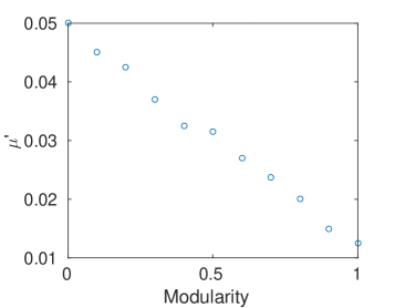
Figure 6: Mutation rate of genetic sequence at which the $F_{\text{ST}}$ ratio is $1.26$ versus modularity . Other parameters are as in Fig. 1.

4 Discussion

So why is having a modular knowledge system so helpful in the human migration process? A migrating human population must adapt knowledge quickly. New knowledge is generated through trial and error (mutation, $\mu$). Communication (knowledge corpus transfer, $\nu$) propagates useful new knowledge in the population. If the knowledge system is non-modular, however, communication causes confusion. This is because transfer of simply a $L/K$ segment does not transfer useful information in a non-modular knowledge system. For example, a hunter can teach a wood gatherer how to hunt, including how to make stone arrowheads. If the knowledge system of the wood gatherer is non-modular, the hunting module can interact with the wood gathering module, and the wood gatherer may wrongly believe that arrow-shaped tools could also work for cutting trees, and replace his or her ax with arrows. For a modular knowledge system, this frustrating confusion will not happen, and modularity reduces frustration. So if the knowledge system is modular, the population can take advantage of faster knowledge communication, while if the system is non-modular, knowledge communication can cause confusion and is deleterious between individuals with different specializations.

For a population with a modular knowledge system, a smaller mutational rate of genes creates the same $F_{\text{ST}}$ ratio, so the evolutionary rate is higher than the non-modular counterpart when the mutational rates are the same. The population with a modular knowledge system evolves faster, and from Fisher’s fundamental theorem of natural selection [32] we expect that the genetic diversity is higher in the more rapidly evolving population.

Why does environmental heterogeneity create an asymmetry of genetic distance in different directions, even if environmental change does not directly influence genes in our model? For a population migrating in the north-south direction, the new environment poses severe challenges to the immigrants, and fewer founders may survive compared to a east-west migration. This founder effect increases the genetic distance between the immigrant population and the population they originate from [33]. For the population migrating in east-west direction, much milder environmental changes largely reduce the founder effect, thus reducing the genetic distance from the original population.

In addition to spatial heterogeneity, our stochastic model naturally creates temporal inhomogeneity. Even though the average fitness of a population changes smoothly, fitness spikes appear occasionally, corresponding to knowledgeable people or "heroes" in human history. Immediately after the initial colonization of one environment, the highest individual fitness value is more than five times the average fitness value of the population in our model. After evolution of the population for approximately $400$ generations, the fitness is "saturated", and the highest fitness is only 50% better than the average fitness. This is consistent with our impression that more heroes emerge in a fast-changing society than a stagnant one.

5 Conclusion

In conclusion, we built a model of population migration in an asymmetric, two dimensional system. We have shown the vital role that modularity plays in the migration rates and gene flows. We have shown that a modular knowledge system coupled with knowledge transfer accelerates human migration. Our results demonstrate an east-west and north-south migration rate difference, and we have related environmental variation with longitude and latitude to migration rate. We have shown that the asymmetry of migration velocity originates from asymmetric environmental gradients. The asymmetry of migration velocity exists only if migration is limited by fitness. Predictions for asymmetry of genetic variation are in agreement with patterns of human gene flow in the Americas. Our model may be applied to other systems such as the spread of invasive species, cancer cells migration, and bacterial migration.

Authors’ contribution

D.W. wrote the codes and collected and analyzed the data. Both D.W. and M.W.D. developed and analyzed the model and drafted the manuscript. All authors gave final approval for publication.

Competing interest

We declare we have no competing interests.

Funding

We received no funding for this study.

Appendix

The dynamics of evolution in one environment is described by a master equation:

$$\frac{dP(\{n_{\bf a}\};t)}{dt} = \sum_{\{{\bf a}\}}\bigg{[}f(S_{\bf a})(n_{\bf a}-1)\sum_{\{{\bf b}\neq{\bf a}\}}\frac{n_{\bf b}+1}{N}P(n_{\bf a}-1,n_{\bf b}+1;t)$$ (12)

$$-f(S_{\bf a})n_{\bf a}\sum_{\{{\bf b}\neq{\bf a}\}}\frac{n_{\bf b}}{N}P(n_{\bf a},n_{\bf b};t)\bigg{]}\delta_{N,N^{*}}$$

$$+\sum_{\{{\bf a}\}}\bigg{[}f(S_{\bf a})(n_{\bf a}-1)P(n_{\bf a}-1;t)-f(S_{\bf a})n_{\bf a}P(n_{\bf a};t)\bigg{]}(1-\delta_{N,N^{*}})$$

$$+\mu\sum_{\{{\bf a}\}}\sum_{\{{\bf b}=\partial{\bf a}\}}\bigg{[}(n_{\bf b}+1)P(n_{\bf a}-1,n_{\bf b}+1;t)-n_{\bf b}P(n_{\bf a},n_{\bf b};t)\bigg{]}$$

$$+\nu\sum_{\{{\bf a}\}}\sum_{k=1}^{K}\sum_{\{{\bf b},{\bf b}_{k}\neq{\bf a}_{k}\}}\bigg{[}(n_{{\bf a}/{\bf b}_{k}}+1)\frac{n_{{\bf b}/{\bf a}_{k}}}{N}P(n_{\bf a}-1,n_{{\bf a}/{\bf b}_{k}}+1;t)$$

$$-n_{{\bf a}/{\bf b}_{k}}\frac{n_{{\bf b}/{\bf a}_{k}}}{N}P(n_{\bf a},n_{{\bf a}/{\bf b}_{k}};t)\bigg{]}$$

Here $n_{\bf a}$ is the number of individuals with sequence $S_{\bf a}$, with the vector index ${\bf a}$ used to label the $2^{L}$ sequences. The notation $\partial{\bf a}$ means the $L$ sequences created by a single mutation from sequence $S_{\bf a}$. The notation ${\bf a}/{\bf b}_{k}$ means the sequence created by transferring module $k$ from sequence $S_{\bf b}$ into sequence $S_{\bf a}$. Here $N^{*}$ is the environmental capacity of the environment.

References

- [1] Hermsen R, Hwa T. Sources and sinks: a stochastic model of evolution in heterogeneous environments. Physical Review Letters. 2010;105:248104. doi:10.1103/PhysRevLett.105.248104.
- [2] Zhang Q, Lambert G, Liao D, Kim H, Robin K, Tung Ck, et al. Acceleration of emergence of bacterial antibiotic resistance in connected microenvironments. Science. 2011;333(6050):1764–1767. doi:10.1126/science.1208747.
- [3] Zhang Q, Austin RH. Physics of cancer: the impact of heterogeneity. Annual Review of Condensed Matter Physics. 2012;3(1):363–382. doi:10.1146/annurev-conmatphys-020911-125109.
- [4] Colizza V, Vespignani A. Invasion threshold in heterogeneous metapopulation networks. Physical Review Letters. 2007;99:148701. doi:10.1103/PhysRevLett.99.148701.
- [5] Türtscher P, von Krogh GF, Gassmann O. The emergence of architecture in modular systems: coordination across boundaries at ATLAS, CERN, Dissertation no. 3578. Norderstedt: Books on Demand GmbH; 2008.
- [6] Kashtan N, Parter M, Dekel E, Mayo AE, Alon U. Extinctions in heterogeneous environments and the evolution of modularity. Evolution. 2009;63(8):1964–1975. doi:10.1111/j.1558-5646.2009.00684.x.
- [7] Doyle AD, Wang FW, Matsumoto K, Yamada KM. One-dimensional topography underlies three-dimensional fibrillar cell migration. The Journal of Cell Biology. 2009;184(4):481–490. doi:10.1083/jcb.200810041.
- [8] Diamond JM. Guns, germs, and steel. W. W. Norton; 1997.
- [9] Steele J. Human dispersals: mathematical models and the archaeological record. Human Biology. 2009;81(3):121–140. doi:10.3378/027.081.0302.
- [10] Anderson DG, Gillam JC. Paleoindian colonization of the Americas: implications from an examination of physiography, demography, and artifact distribution. American Antiquity. 2000;p. 43–66. doi:10.2307/2694807.
- [11] Campbell DT. Blind variation and selective retentions in creative thought as in other knowledge processes. Psychological Review. 1960;67(6):380. doi:10.1037/h0040373.
- [12] Mithen SJ. The prehistory of the mind : a search for the origins of art, religion, and science. London : Thames and Hudson; 1996.
- [13] Kandler A, Steele J. Social learning, economic inequality, and innovation diffusion. In: Innovation in cultural systems: Contributions from evolutionary anthropology. The MIT Press; 2010. p. 193–214.
- [14] Steele J. Weak modularity and the evolution of human social behavior. In: Darwinian archaeologies. Springer; 1996. p. 185–195.
- [15] Tooby J, Cosmides L. The psychological foundations of culture. In: Barkow JH, Cosmides L, Tooby J, editors. The adapted mind: Evolutionary psychology and the generation of culture. Oxford University Press Oxford; 1995. p. 19–136.
- [16] Goldenfeld N, Woese C. Life is physics: evolution as a collective phenomenon far from equilibrium. Annual Review of Condensed Matter Physics. 2011;2:375–399. doi:10.1146/annurev-conmatphys-062910-140509.
- [17] Deem MW. Statistical mechanics of modularity and horizontal gene transfer. Annual Review of Condensed Matter Physics. 2013;4:287–311. doi:10.1146/annurev-conmatphys-030212-184316.
- [18] Kottek M, Grieser J, Beck C, Rudolf B, Rubel F. World map of the Köppen-Geiger climate classification updated. Meteorologische Zeitschrift. 2006;15(3):259–263. doi:10.1127/0941-2948/2006/0130.
- [19] Hui C. Carrying capacity, population equilibrium, and environment’s maximal load. Ecological Modelling. 2006;192(1):317–320. doi:10.1016/j.ecolmodel.2005.07.001.
- [20] Maddison A. The world economy. Academic Foundation; 2007.
- [21] Nunes S, Holekamp KE. Mass and fat influence the timing of natal dispersal in Belding’s ground squirrels. Journal of Mammalogy. 1996;77(3):807–817. doi:10.2307/1382686.
- [22] O’Riain MJ, Jarvis JU, Faulkesi CG. A dispersive morph in the naked mole-rat. Nature. 1996;380:18. doi:10.1038/380619a0.
- [23] Wang S, Lewis Jr CM, Jakobsson M, Ramachandran S, Ray N, Bedoya G, et al. Genetic variation and population structure in Native Americans. PLoS Genet. 2007;3(11):e185. doi:10.1371/journal.pgen.0030185.
- [24] Goebel T, Waters MR, O’Rourke DH. The late Pleistocene dispersal of modern humans in the Americas. Science. 2008;319(5869):1497–1502. doi:10.1126/science.1153569.
- [25] Park JM, Chen M, Wang D, Deem MW. Modularity enhances the rate of evolution in a rugged fitness landscape. Physical Biology. 2015;12(2):025001. doi:10.1088/1478-3975/12/2/025001.
- [26] Ramachandran S, Rosenberg NA. A test of the influence of continental axes of orientation on patterns of human gene flow. American Journal of Physical Anthropology. 2011;146(4):515–529. doi:10.1002/ajpa.21533.
- [27] Sun J, Deem MW. Spontaneous emergence of modularity in a model of evolving individuals. Physical Review Letters. 2007;99:228107. doi:10.1103/PhysRevLett.99.228107.
- [28] Wigner EP. On the distribution of the roots of certain symmetric matrices. Annals of Mathematics. 1958;p. 325–327. doi:10.2307/1970008.
- [29] Sadoc JF, Mosseri R. Geometrical frustration. Cambridge University Press; 2006.
- [30] Weir BS. Genetic data analysis II. methods for discrete population genetic data. Sinauer Associates, Inc. Publishers; 1996.
- [31] Kayser M, Roewer L, Hedman M, Henke L, Henke J, Brauer S, et al. Characteristics and frequency of germline mutations at microsatellite loci from the human Y chromosome, as revealed by direct observation in father/son pairs. The American Journal of Human Genetics. 2000;66(5):1580–1588. doi:10.1086/302905.
- [32] Fisher RA. The genetical theory of natural selection: a complete variorum edition. Oxford University Press; 1930.
- [33] Hedrick PW. Genetics of populations. Jones & Bartlett Learning; 2011.