A note on simple randomly switched linear systems

Gabriel LAGASQUIE
Abstract

We construct a planar process that switches randomly between the flows of two linear systems built from two Hurwitz matrices (all eigenvalues have negative real parts). The goal here is to study the long time behaviour according to the switching rates. We will see that, even if the two systems are stable, it is possible to obtain a blow up if we choose the switching rates wisely. Finally we will see a connection, between the tail of the invariant measure (when the switching times follow an exponential law) and the existence of a deterministic control that makes the process explode.

AMS Classification: 60J99, 34A60

1 Introduction

Piecewise Deterministic Markov Processes (PDMPs) is a huge class of stochastic processes introduced by Davis [8]. In this note we are studying a particular subclass of these processes. we consider (Xt,It)tโฉพ0subscriptsubscript๐‘‹๐‘กsubscript๐ผ๐‘ก๐‘ก0(X_{t},I_{t})_{t\geqslant 0} evolving on the space โ„dร—{0,1}superscriptโ„๐‘‘01\mathbb{R}^{d}\times\{0,1\} solving the equation:

Xห™t=Fโ€‹(Xt,It)subscriptห™๐‘‹๐‘ก๐นsubscript๐‘‹๐‘กsubscript๐ผ๐‘ก\dot{X}_{t}=F(X_{t},I_{t})

where F๐นF is a smooth function and (It)subscript๐ผ๐‘ก(I_{t}) is a jump process on {0,1}01\{0,1\}. We call ฮปisubscript๐œ†๐‘–\lambda_{i} the jump rate of the process (It)subscript๐ผ๐‘ก(I_{t}) from state i๐‘–i to state 1โˆ’i1๐‘–1-i. Such processes play a role in modeling problems in various fields such as molecular biology [13], population dynamics [7], Internet traffic [10]. Even if these processes are easy to define, their stability is never clear.

More precisely, we are here interested in the long time qualitative behaviour of the planar randomly switched process (Xt,It)tโฉพ0โˆˆโ„dร—{0,1}subscriptsubscript๐‘‹๐‘กsubscript๐ผ๐‘ก๐‘ก0superscriptโ„๐‘‘01(X_{t},I_{t})_{t\geqslant 0}\in\mathbb{R}^{d}\times\{0,1\} solving the equation

{Xห™t=AItโ€‹XtX0=x0,\left\{\begin{aligned} &\dot{X}_{t}=A_{I_{t}}X_{t}\\ &X_{0}=x_{0},\end{aligned}\right. (1)

where A0subscript๐ด0A_{0}, A1subscript๐ด1A_{1} are dร—d๐‘‘๐‘‘d\times d real matrices, and (It)subscript๐ผ๐‘ก(I_{t}) is a Markov process on E={0,1}๐ธ01E=\{0,1\} with constant jump rates:

ฮป0=ฮฒโ€‹u,subscript๐œ†0๐›ฝ๐‘ข\displaystyle\lambda_{0}=\beta u,
ฮป1=ฮฒโ€‹(1โˆ’u)subscript๐œ†1๐›ฝ1๐‘ข\displaystyle\lambda_{1}=\beta(1-u)

where ฮฒ>0๐›ฝ0\beta>0 and uโˆˆ(0,1)๐‘ข01u\in(0,1). The process ((Xt,It))tโ‰ฅ0subscriptsubscript๐‘‹๐‘กsubscript๐ผ๐‘ก๐‘ก0((X_{t},I_{t}))_{t\geq 0} is a piecewise deterministic Markov process as defined in [8] and several examples have been studied in [12] or [5]. It appears that the following quantity dictates the large time behaviour of this process according to the parameters A0subscript๐ด0A_{0}, A1subscript๐ด1A_{1}, ฮฒ๐›ฝ\beta and u๐‘ขu:

ฯ‡:=ฯ‡โ€‹(A0,A1,ฮฒ,u)=limtโ†’+โˆžโ€‹1tโ€‹logโก(โ€–Xtโ€–)a.s.formulae-sequenceassign๐œ’๐œ’subscript๐ด0subscript๐ด1๐›ฝ๐‘ขโ†’๐‘ก1๐‘กnormsubscript๐‘‹๐‘กa.s\chi:=\chi(A_{0},A_{1},\beta,u)=\underset{t\rightarrow+\infty}{\lim}\frac{1}{t}\log\left(\|X_{t}\|\right)\quad\text{a.s}.

Indeed if ฯ‡๐œ’\chi is positive then the system explodes almost surely whereas if ฯ‡๐œ’\chi is negative the system is stable and goes to zero almost surely.

The asymptotic behaviour of such processes when (It)subscript๐ผ๐‘ก(I_{t}) is any deterministic process and d=2๐‘‘2d=2 is now understood. Given two matrices in โ„ณ2โ€‹(โ„)subscriptโ„ณ2โ„\mathcal{M}_{2}(\mathbb{R}), [3] gives a necessary and sufficient condition for the existence of a deterministic function (It)subscript๐ผ๐‘ก(I_{t}) that produces a blow up. But the articles [12] and [6] have shown that the behaviour of planar randomly switched systems may be surprising: according to the value of the switching rate ฮฒ๐›ฝ\beta, the process can either blow up or go to zero even if each system is stable. In [12], the authors build a randomly switched system living in the space โ„2โ€‹nsuperscriptโ„2๐‘›\mathbb{R}^{2n} which behaviour comes down to alternating blow up periods and stable periods a finite number of times as the jump rate grows.

A question raised from these works is the existence of a planar randomly switched system which behaviour is also alternating between blow up periods and stable periods. The goal of this note is to construct such a process.
Our idea is the following: put a stochastic control in a deterministic planar switched system which satisfies the qualitative long time behaviour condition (using the criteria in [3]). For a>0๐‘Ž0a>0 and b>1๐‘1b>1, we define two real matrices as follow:

A0=(โˆ’abโˆ’1bโˆ’a)andA1=(โˆ’a1bโˆ’bโˆ’a).formulae-sequencesubscript๐ด0matrix๐‘Ž๐‘1๐‘๐‘Žandsubscript๐ด1matrix๐‘Ž1๐‘๐‘๐‘ŽA_{0}=\begin{pmatrix}-a&b\\ -\frac{1}{b}&-a\end{pmatrix}\quad\text{and}\quad A_{1}=\begin{pmatrix}-a&\frac{1}{b}\\ -b&-a\end{pmatrix}.

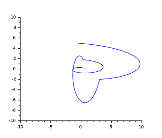
Thanks to these two matrices, we define the continuous process ((Xt,It))tโ‰ฅ0โˆˆโ„2ร—{0,1}subscriptsubscript๐‘‹๐‘กsubscript๐ผ๐‘ก๐‘ก0superscriptโ„201((X_{t},I_{t}))_{t\geq 0}\in\mathbb{R}^{2}\times\{0,1\} solution of (1). The path of Xtsubscript๐‘‹๐‘กX_{t} follows a spiral clockwisely during a random time with exponential law of parameter ฮปisubscript๐œ†๐‘–\lambda_{i} before switching on an other spiral as described in Figure 1.
Refer to caption
Figure 1: Example of a trajectory of the process (1).

We also define:

ฯ‡:=ฯ‡โ€‹(a,b,ฮฒ,u)=limtโ†’+โˆžโ€‹1tโ€‹logโก(โ€–Xtโ€–)a.sformulae-sequenceassign๐œ’๐œ’๐‘Ž๐‘๐›ฝ๐‘ขโ†’๐‘ก1๐‘กnormsubscript๐‘‹๐‘กa.s\chi:=\chi(a,b,\beta,u)=\underset{t\rightarrow+\infty}{\lim}\frac{1}{t}\log\left(\|X_{t}\|\right)\quad\text{a.s}

which sign gives the long time qualitative behaviour of our process as said before.

The main result of this note is the following which is similar to the main result in [12]:

Theorem 1.1.

For any uโˆˆ(0,1)๐‘ข01u\in(0,1),

(i)โˆ€a,b>0,ฯ‡โ€‹(a,b,ฮฒ,u)โŸถโˆ’aโ€‹ย whenย โ€‹ฮฒโ†’0โ€‹ย orย โ€‹ฮฒโ†’+โˆž.formulae-sequence๐‘–for-all๐‘Ž๐‘0โŸถ๐œ’๐‘Ž๐‘๐›ฝ๐‘ข๐‘Žย whenย ๐›ฝโ†’0ย orย ๐›ฝโ†’\displaystyle(i)\quad\forall a,b>0,\quad\chi(a,b,\beta,u)\longrightarrow-a\text{ when }\beta\rightarrow 0\text{ or }\beta\rightarrow+\infty.
(iโ€‹i)For everyย โ€‹ฮฒ,u>0โ€‹ย there existย โ€‹a>0โ€‹ย andย โ€‹b>0โ€‹ย so thatย โ€‹ฯ‡โ€‹(a,b,ฮฒ,u)>0.๐‘–๐‘–For everyย ๐›ฝ๐‘ข0ย there existย ๐‘Ž0ย andย ๐‘0ย so thatย ๐œ’๐‘Ž๐‘๐›ฝ๐‘ข0\displaystyle(ii)\quad\text{For every }\beta,u>0\text{ there exist }a>0\text{ and }b>0\text{ so that }\chi(a,b,\beta,u)>0.

In Section 2, we establish an explicit expression of the function ฯ‡๐œ’\chi. In Section 3 we use it to prove Theorem 1.1.

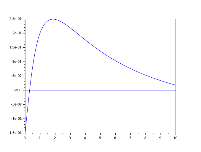
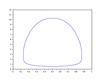
The explicit expression of ฯ‡๐œ’\chi obtained in Proposition 2.2 allows us to calculate numerically the function ฯ‡๐œ’\chi at u๐‘ขu constant (see Figure 2). It is also interesting to show the sign of the function ฯ‡๐œ’\chi according to ฮฒ๐›ฝ\beta and u๐‘ขu as we can see in Figure 3. In this figure, we can see that for (ฮฒ,u)๐›ฝ๐‘ข(\beta,u) in a compact, our system explodes when t๐‘กt goes to +โˆž+\infty. We can see the same behaviour in the process studied in [12]. But this is different from what we can observe in [7] and [6] where the explosion happens for ฮฒ๐›ฝ\beta large enough.

Refer to caption
Figure 2: The function ฯ‡๐œ’\chi for a=0.15๐‘Ž0.15a=0.15, b=3๐‘3b=3 and u=0.5๐‘ข0.5u=0.5.
Refer to caption
Figure 3: Sign of the function ฯ‡๐œ’\chi for a=0.10๐‘Ž0.10a=0.10, b=2.5๐‘2.5b=2.5. Positive inside and negative outside.

This graphics combined to Theorem 1.1 shows us that this process does not meet our expectations. There is a unique area of blow up whereas the deterministic periodic process has several blow up periods (see Section 4). It seems that, in the case of the random process, the variance of the waiting time in each state is too high to select precisely the good jump times that would allow it to have several blow up periods.

We will see in Section 5 a simple way to lower the variance of the waiting time without complicate too much the process, but first, in Section 4 we will give an interesting result about the deterministic process associated to our system.

In the last section we focus on the decentered switched system defined as follow:

{Xห™t=AItโ€‹(Xtโˆ’bIt)X0=x0,\left\{\begin{aligned} &\dot{X}_{t}=A_{I_{t}}(X_{t}-b_{I_{t}})\\ &X_{0}=x_{0},\end{aligned}\right. (2)

where b0subscript๐‘0b_{0}, b1subscript๐‘1b_{1} are two different vectors of โ„dsuperscriptโ„๐‘‘\mathbb{R}^{d}.
There is a connection between the existence of an explosive trajectory (with a deterministic control) and the properties of the invariant measure, if it exists, in the random case (exponential switch times).

Let us call T0=0subscript๐‘‡00T_{0}=0, T1subscript๐‘‡1T_{1}, โ€ฆ, Tnsubscript๐‘‡๐‘›T_{n} the jumping times of the process (Xt)subscript๐‘‹๐‘ก(X_{t}) and ฯ„0subscript๐œ0\tau_{0}, ฯ„1subscript๐œ1\tau_{1}, โ€ฆ, ฯ„nsubscript๐œ๐‘›\tau_{n}, the interjump times following an exponential law of parameters ฮป0subscript๐œ†0\lambda_{0} and ฮป1subscript๐œ†1\lambda_{1} alternatively. Let us define Yn=XT2โ€‹nsubscript๐‘Œ๐‘›subscript๐‘‹subscript๐‘‡2๐‘›Y_{n}=X_{T_{2n}}. By simply solving the equation 2 between each jumping times we obtain:

Yn=eฯ„n+1โ€‹A1โ€‹eฯ„nโ€‹A0โ€‹Ynโˆ’1โˆ’eฯ„n+1โ€‹b0+b1.subscript๐‘Œ๐‘›superscript๐‘’subscript๐œ๐‘›1subscript๐ด1superscript๐‘’subscript๐œ๐‘›subscript๐ด0subscript๐‘Œ๐‘›1superscript๐‘’subscript๐œ๐‘›1subscript๐‘0subscript๐‘1Y_{n}=e^{\tau_{n+1}A_{1}}e^{\tau_{n}A_{0}}Y_{n-1}-e^{\tau_{n+1}}b_{0}+b_{1}.

This kind of stochastic equation have been the object of numerous research. Applying Kestenโ€™s renewal theorem to the discrete process (Yn)subscript๐‘Œ๐‘›(Y_{n}) will give some informations about the tail of the invariant measure of (Xt)subscript๐‘‹๐‘ก(X_{t}) (see [11] for the main article, see [1], [9] for different formulations of the same theorem).

Theorem 1.2.

If there is no deterministic control that makes the deterministic process associated to (Yt(Y_{t}) explodes, it means that there exists an invariant measure ฮผ๐œ‡\mu for our process and the support of ฮผ๐œ‡\mu is necessarily bounded.

In the other hand, we assume that ฯ‡<0๐œ’0\chi<0 and that there exists a deterministic control such as:

โˆƒkโˆˆ2โ€‹โ„•+1โ€‹ย such asย โ€‹โˆ€xโˆˆ๐•Šdโˆ’1,โˆƒt0,t1,โ€ฆ,tk>0โ€‹ย such asย โ€‹โ€–etkโ€‹AIkโ€‹โ€ฆโ€‹et1โ€‹AI1โ€‹et0โ€‹AI0โ€‹xโ€–>โ€–xโ€–.formulae-sequence๐‘˜2โ„•1ย such asย for-all๐‘ฅsubscript๐•Š๐‘‘1subscript๐‘ก0subscript๐‘ก1โ€ฆsubscript๐‘ก๐‘˜0ย such asย normsuperscript๐‘’subscript๐‘ก๐‘˜subscript๐ดsubscript๐ผ๐‘˜โ€ฆsuperscript๐‘’subscript๐‘ก1subscript๐ดsubscript๐ผ1superscript๐‘’subscript๐‘ก0subscript๐ดsubscript๐ผ0๐‘ฅnorm๐‘ฅ\exists k\in 2\mathbb{N}+1\text{ such as }\forall x\in\mathbb{S}_{d-1},\exists t_{0},t_{1},...,t_{k}>0\text{ such as }\|e^{t_{k}A_{I_{k}}}...e^{t_{1}A_{I_{1}}}e^{t_{0}A_{I_{0}}}x\|>\|x\|. (3)

We call B=eฯ„kโ€‹AIkโ€‹โ€ฆโ€‹eฯ„1โ€‹AI1โ€‹eฯ„0โ€‹AI0๐ตsuperscript๐‘’subscript๐œ๐‘˜subscript๐ดsubscript๐ผ๐‘˜โ€ฆsuperscript๐‘’subscript๐œ1subscript๐ดsubscript๐ผ1superscript๐‘’subscript๐œ0subscript๐ดsubscript๐ผ0B=e^{\tau_{k}A_{I_{k}}}...e^{\tau_{1}A_{I_{1}}}e^{\tau_{0}A_{I_{0}}} and B0subscript๐ต0B_{0}, B1subscript๐ต1B_{1}, โ€ฆ, Bnsubscript๐ต๐‘›B_{n} n๐‘›n random variables i.i.d following the law of B๐ตB. We also assume that:

maxnโฉพ0โ€‹ย โ€‹โ„™โ€‹(Bnโ€‹โ€ฆโ€‹B0โ€‹xโ€–Bnโ€‹โ€ฆโ€‹B0โ€‹xโ€–โˆˆU)>0โ€‹ย for allย โ€‹xโˆˆ๐•Šdโˆ’1โ€‹ย and any openย โ€‹โˆ…โ‰ UโŠ‚๐•Šdโˆ’1.๐‘›0ย โ„™subscript๐ต๐‘›โ€ฆsubscript๐ต0๐‘ฅnormsubscript๐ต๐‘›โ€ฆsubscript๐ต0๐‘ฅ๐‘ˆ0ย for allย ๐‘ฅsubscript๐•Š๐‘‘1ย and any openย ๐‘ˆsubscript๐•Š๐‘‘1\underset{n\geqslant 0}{\max}\text{ }\mathbb{P}\left(\frac{B_{n}...B_{0}x}{\|B_{n}...B_{0}x\|}\in U\right)>0\text{ for all }x\in\mathbb{S}_{d-1}\text{ and any open }\emptyset\neq U\subset\mathbb{S}_{d-1}. (4)
โ„™(Bn0โ€ฆB0โˆˆ.)โฉพฮณ0๐Ÿ™Bcโ€‹(ฮ“0)ฮปย for someย ฮ“0โˆˆGLd(โ„),ย n0โˆˆโ„•ย andย c,ฮณ0>0.\mathbb{P}(B_{n_{0}}...B_{0}\in.)\geqslant\gamma_{0}\mathds{1}_{B_{c}(\Gamma_{0})}\lambda\text{ for some }\Gamma_{0}\in GL_{d}(\mathbb{R}),\text{ }n_{0}\in\mathbb{N}\text{ and }c,\gamma_{0}>0. (5)

where ฮป๐œ†\lambda is the Lebesgue measure on โ„n2superscriptโ„superscript๐‘›2\mathbb{R}^{n^{2}}. Under these assumptions, there exists a unique invariant measure ฮผ๐œ‡\mu for the process (Yt)subscript๐‘Œ๐‘ก(Y_{t}) and it has an heavy tail:

โˆƒp1>0โ€‹ย such asย โ€‹โˆ€0โฉฝp<p1๐”ผฮผโ€‹[โ€–Yโ€–p]โ€‹<+โˆžโ€‹ย andย โ€‹โˆ€p>โ€‹p1๐”ผฮผโ€‹[โ€–Yโ€–p]=+โˆž.formulae-sequencesubscript๐‘10ย such asย for-all0๐‘subscript๐‘1subscript๐”ผ๐œ‡delimited-[]superscriptnorm๐‘Œ๐‘expectationย andย for-all๐‘subscript๐‘1subscript๐”ผ๐œ‡delimited-[]superscriptnorm๐‘Œ๐‘\exists p_{1}>0\text{ such as }\forall 0\leqslant p<p_{1}\quad\mathbb{E}_{\mu}[\|Y\|^{p}]<+\infty\text{ and }\forall p>p_{1}\quad\mathbb{E}_{\mu}[\|Y\|^{p}]=+\infty.

2 Study of the angular process

In order to study our process ((Xt,It))tโ‰ฅ0subscriptsubscript๐‘‹๐‘กsubscript๐ผ๐‘ก๐‘ก0((X_{t},I_{t}))_{t\geq 0} we use the polar coordinates for Xtsubscript๐‘‹๐‘กX_{t}. As a start, and as in [12], let us look at the case of the deterministic process. Let A๐ดA be a 2-sized squared matrix and xโˆˆโ„2\{0}๐‘ฅ\superscriptโ„20x\in\mathbb{R}^{2}\backslash\{0\}. We set (xt)tโ‰ฅ0subscriptsubscript๐‘ฅ๐‘ก๐‘ก0(x_{t})_{t\geq 0} the solution of the ODE:

{xห™t=Aโ€‹xtfor allย โ€‹t>0,x0=x.casesformulae-sequencesubscriptห™๐‘ฅ๐‘ก๐ดsubscript๐‘ฅ๐‘กfor allย ๐‘ก0missing-subexpressionsubscript๐‘ฅ0๐‘ฅmissing-subexpression\left\{\begin{array}[]{ll}\dot{x}_{t}=Ax_{t}\quad\text{for all }t>0,\\ x_{0}=x.\end{array}\right.

If x๐‘ฅx is nonzero, then it is also true for any xtsubscript๐‘ฅ๐‘กx_{t} with t๐‘กt positive. So we can define the polar coordinates (rt,ฮธt)subscript๐‘Ÿ๐‘กsubscript๐œƒ๐‘ก(r_{t},\theta_{t}) of xtsubscript๐‘ฅ๐‘กx_{t}. We call eฮธsubscript๐‘’๐œƒe_{\theta} the unitary vector (cosโกฮธ,sinโกฮธ)๐œƒ๐œƒ(\cos\theta,\sin\theta) and ut=eฮธtsubscript๐‘ข๐‘กsubscript๐‘’subscript๐œƒ๐‘กu_{t}=e_{\theta_{t}}. Then xt=rtโ€‹utsubscript๐‘ฅ๐‘กsubscript๐‘Ÿ๐‘กsubscript๐‘ข๐‘กx_{t}=r_{t}u_{t}. As rt2=โŸจxt,xtโŸฉsuperscriptsubscript๐‘Ÿ๐‘ก2subscript๐‘ฅ๐‘กsubscript๐‘ฅ๐‘กr_{t}^{2}={{\left<x_{t},x_{t}\right>}}, we obtain the relations:

rtโ€‹rห™t=โŸจxt,Aโ€‹xtโŸฉsubscript๐‘Ÿ๐‘กsubscriptห™๐‘Ÿ๐‘กsubscript๐‘ฅ๐‘ก๐ดsubscript๐‘ฅ๐‘กr_{t}\dot{r}_{t}={{\left<x_{t},Ax_{t}\right>}}
Aโ€‹(rtโ€‹ut)=xห™t=rห™tโ€‹ut+rtโ€‹uห™t.๐ดsubscript๐‘Ÿ๐‘กsubscript๐‘ข๐‘กsubscriptห™๐‘ฅ๐‘กsubscriptห™๐‘Ÿ๐‘กsubscript๐‘ข๐‘กsubscript๐‘Ÿ๐‘กsubscriptห™๐‘ข๐‘กA(r_{t}u_{t})=\dot{x}_{t}=\dot{r}_{t}u_{t}+r_{t}\dot{u}_{t}.

And then we have:

rห™t=rtโ€‹โŸจut,Aโ€‹utโŸฉsubscriptห™๐‘Ÿ๐‘กsubscript๐‘Ÿ๐‘กsubscript๐‘ข๐‘ก๐ดsubscript๐‘ข๐‘ก\dot{r}_{t}=r_{t}{{\left<u_{t},Au_{t}\right>}} (6)
uห™t=Aโ€‹utโˆ’โŸจut,Aโ€‹utโŸฉโ€‹ut.subscriptห™๐‘ข๐‘ก๐ดsubscript๐‘ข๐‘กsubscript๐‘ข๐‘ก๐ดsubscript๐‘ข๐‘กsubscript๐‘ข๐‘ก\dot{u}_{t}=Au_{t}-{{\left<u_{t},Au_{t}\right>}}u_{t}. (7)

Let us write the equation (2) with the angle ฮธtsubscript๐œƒ๐‘ก\theta_{t}. As uห™t=ฮธห™tโ€‹eฮธt+ฯ€/2subscriptห™๐‘ข๐‘กsubscriptห™๐œƒ๐‘กsubscript๐‘’subscript๐œƒ๐‘ก๐œ‹2\dot{u}_{t}=\dot{\theta}_{t}e_{\theta_{t}+\pi/2}, by making the scalar product of (2) with eฮธt+ฯ€/2subscript๐‘’subscript๐œƒ๐‘ก๐œ‹2e_{\theta_{t}+\pi/2}, we obtain:

ฮธห™t=โŸจAโ€‹eฮธt,eฮธt+ฯ€/2โŸฉ.subscriptห™๐œƒ๐‘ก๐ดsubscript๐‘’subscript๐œƒ๐‘กsubscript๐‘’subscript๐œƒ๐‘ก๐œ‹2\dot{\theta}_{t}={{\left<Ae_{\theta_{t}},e_{\theta_{t}+\pi/2}\right>}}. (8)

We use now the polar coordinates in order to study the process ((Xt,It))tโ‰ฅ0subscriptsubscript๐‘‹๐‘กsubscript๐ผ๐‘ก๐‘ก0((X_{t},I_{t}))_{t\geq 0}. Between the jumps, the process follows the flow determined by Aโˆˆ{A0,A1}๐ดsubscript๐ด0subscript๐ด1A\in\{A_{0},A_{1}\}. From Equation (3), the development of ฮธ๐œƒ\theta is deterministic and does not depend on r๐‘Ÿr. As a consequence, the processes ((ฮ˜t,It))tโ‰ฅ0subscriptsubscriptฮ˜๐‘กsubscript๐ผ๐‘ก๐‘ก0((\Theta_{t},I_{t}))_{t\geq 0} and ((Ut,It))tโ‰ฅ0subscriptsubscript๐‘ˆ๐‘กsubscript๐ผ๐‘ก๐‘ก0((U_{t},I_{t}))_{t\geq 0} are piecewise deterministic Markov processes on โ„ร—{0,1}โ„01\mathbb{R}\times\{0,1\} and ๐•Š1ร—{0,1}subscript๐•Š101\mathbb{S}_{1}\times\{0,1\} respectively. The principal interest of the study of these processes lies in the fact that the development of (Rt)tโ‰ฅ0subscriptsubscript๐‘…๐‘ก๐‘ก0(R_{t})_{t\geq 0} is determined by that of the process ((ฮ˜t,It))tโ‰ฅ0subscriptsubscriptฮ˜๐‘กsubscript๐ผ๐‘ก๐‘ก0((\Theta_{t},I_{t}))_{t\geq 0} as shown by Equation (1). Indeed, by solving (1) between the jumps and by calling ๐’œโ€‹(ฮธ,i)=โŸจAiโ€‹eฮธ,eฮธโŸฉ๐’œ๐œƒ๐‘–subscript๐ด๐‘–subscript๐‘’๐œƒsubscript๐‘’๐œƒ\mathcal{A}(\theta,i)={{\left<A_{i}e_{\theta},e_{\theta}\right>}}, we obtain:

Rt=R0โ€‹expโก(โˆซ0t๐’œโ€‹(ฮ˜s,Is)โ€‹๐‘‘s).subscript๐‘…๐‘กsubscript๐‘…0superscriptsubscript0๐‘ก๐’œsubscriptฮ˜๐‘ subscript๐ผ๐‘ differential-d๐‘ R_{t}=R_{0}\exp\left(\int_{0}^{t}\mathcal{A}(\Theta_{s},I_{s})ds\right). (9)

So, as suggested by Equation (4), in order to study the behaviour of (Rt)tโ‰ฅ0subscriptsubscript๐‘…๐‘ก๐‘ก0(R_{t})_{t\geq 0} we are going to study the process ((ฮ˜t,It))tโ‰ฅ0subscriptsubscriptฮ˜๐‘กsubscript๐ผ๐‘ก๐‘ก0((\Theta_{t},I_{t}))_{t\geq 0} and particularly its invariant measure.

Lemma 2.1.

The invariant measure ฮผ๐œ‡\mu of the process ((ฮ˜t,It))tโ‰ฅ0subscriptsubscriptฮ˜๐‘กsubscript๐ผ๐‘ก๐‘ก0((\Theta_{t},I_{t}))_{t\geq 0} is given by,

ฮผโ€‹(dโ€‹ฮธ,i)=ฯiโ€‹(ฮธ)โ€‹dโ€‹ฮธ๐œ‡๐‘‘๐œƒ๐‘–subscript๐œŒ๐‘–๐œƒ๐‘‘๐œƒ\mu(d\theta,i)=\rho_{i}(\theta)d\theta

where:

ฯ0=ฮฆd0andฯ1=Cโˆ’ฯ0โ€‹d0d1;formulae-sequencesubscript๐œŒ0ฮฆsubscript๐‘‘0andsubscript๐œŒ1๐ถsubscript๐œŒ0subscript๐‘‘0subscript๐‘‘1\displaystyle\rho_{0}=\frac{\Phi}{d_{0}}\quad\text{and}\quad\rho_{1}=\frac{C-\rho_{0}d_{0}}{d_{1}};
d0โ€‹(ฮธ)=โˆ’bโ€‹sin2โก(ฮธ)โˆ’1bโ€‹cos2โก(ฮธ)andd1โ€‹(ฮธ)=โˆ’1bโ€‹sin2โก(ฮธ)โˆ’bโ€‹cos2โก(ฮธ);formulae-sequencesubscript๐‘‘0๐œƒ๐‘superscript2๐œƒ1๐‘superscript2๐œƒandsubscript๐‘‘1๐œƒ1๐‘superscript2๐œƒ๐‘superscript2๐œƒ\displaystyle d_{0}(\theta)=-b\sin^{2}(\theta)-\frac{1}{b}\cos^{2}(\theta)\quad\text{and}\quad d_{1}(\theta)=-\frac{1}{b}\sin^{2}(\theta)-b\cos^{2}(\theta);
ฮฆโ€‹(ฮธ)=(K+โˆซ0ฮธฮฒโ€‹Cโ€‹(1โˆ’u)โ€‹1d1โ€‹(ฮฑ)โ€‹eโˆ’ฮฒโ€‹vโ€‹(ฮฑ)โ€‹๐‘‘ฮฑ)โ€‹eฮฒโ€‹vโ€‹(ฮธ);ฮฆ๐œƒ๐พsuperscriptsubscript0๐œƒ๐›ฝ๐ถ1๐‘ข1subscript๐‘‘1๐›ผsuperscript๐‘’๐›ฝ๐‘ฃ๐›ผdifferential-d๐›ผsuperscript๐‘’๐›ฝ๐‘ฃ๐œƒ\displaystyle\Phi(\theta)=\left(K+\int_{0}^{\theta}\beta C(1-u)\frac{1}{d_{1}(\alpha)}e^{-\beta v(\alpha)}d\alpha\right)e^{\beta v(\theta)};
vโ€‹ย is the primitive null in zero of the functionย โˆ’(ud0+1โˆ’ud1);๐‘ฃย is the primitive null in zero of the functionย ๐‘ขsubscript๐‘‘01๐‘ขsubscript๐‘‘1\displaystyle v\text{ is the primitive null in zero of the function }-(\frac{u}{d_{0}}+\frac{1-u}{d_{1}});
Kโ€‹ย andย โ€‹Cโ€‹ย are two explicit constants.๐พย andย ๐ถย are two explicit constants.\displaystyle K\text{ and }C\text{ are two explicit constants.}
Proof.

We define, for iโˆˆ{0,1}๐‘–01i\in\{0,1\},

diโ€‹(ฮธ)=โŸจAiโ€‹eฮธ,eฮธ+ฯ€/2โŸฉ.subscript๐‘‘๐‘–๐œƒsubscript๐ด๐‘–subscript๐‘’๐œƒsubscript๐‘’๐œƒ๐œ‹2d_{i}(\theta)={{\left<A_{i}e_{\theta},e_{\theta+\pi/2}\right>}}.

We call L๐ฟL the infinitesimal generator associated to the semi-group Ptsubscript๐‘ƒ๐‘กP_{t} of the process ((ฮ˜t,It))tโ‰ฅ0subscriptsubscriptฮ˜๐‘กsubscript๐ผ๐‘ก๐‘ก0((\Theta_{t},I_{t}))_{t\geq 0}. Remind that Pt=Eโ€‹[fโ€‹(ฮ˜t,It)|ฮ˜0=ฮธ,I0=i]subscript๐‘ƒ๐‘ก๐ธdelimited-[]formulae-sequenceconditional๐‘“subscriptฮ˜๐‘กsubscript๐ผ๐‘กsubscriptฮ˜0๐œƒsubscript๐ผ0๐‘–P_{t}=E[f(\Theta_{t},I_{t})|\Theta_{0}=\theta,I_{0}=i]. L๐ฟL is given by:

Lโ€‹fโ€‹(ฮธ,i)=diโ€‹(ฮธ)โ€‹โˆ‚fโˆ‚ฮธโ€‹(ฮธ,i)+ฮปiโ€‹(fโ€‹(ฮธ,1โˆ’i)โˆ’fโ€‹(ฮธ,i))๐ฟ๐‘“๐œƒ๐‘–subscript๐‘‘๐‘–๐œƒ๐‘“๐œƒ๐œƒ๐‘–subscript๐œ†๐‘–๐‘“๐œƒ1๐‘–๐‘“๐œƒ๐‘–Lf(\theta,i)=d_{i}(\theta)\frac{\partial f}{\partial\theta}(\theta,i)+\lambda_{i}\left(f(\theta,1-i)-f(\theta,i)\right) (10)

for any smooth function f๐‘“f.
In our study case, the functions disubscript๐‘‘๐‘–d_{i} are given by,

d0โ€‹(ฮธ)=โˆ’bโ€‹sin2โกฮธโˆ’1bโ€‹cos2โกฮธandd1โ€‹(ฮธ)=โˆ’1bโ€‹sin2โกฮธโˆ’bโ€‹cos2โกฮธ.formulae-sequencesubscript๐‘‘0๐œƒ๐‘superscript2๐œƒ1๐‘superscript2๐œƒandsubscript๐‘‘1๐œƒ1๐‘superscript2๐œƒ๐‘superscript2๐œƒd_{0}(\theta)=-b\sin^{2}\theta-\frac{1}{b}\cos^{2}\theta\quad\text{and}\quad d_{1}(\theta)=-\frac{1}{b}\sin^{2}\theta-b\cos^{2}\theta.

We notice that the functions disubscript๐‘‘๐‘–d_{i} are negative. This obviously implies that the process ((Ut,It))tโ‰ฅ0subscriptsubscript๐‘ˆ๐‘กsubscript๐ผ๐‘ก๐‘ก0((U_{t},I_{t}))_{t\geq 0} is recurrent, irreducible and it has a unique invariant measure. We want to write it as follows:

ฮผโ€‹(dโ€‹ฮธ,i)=ฯiโ€‹(ฮธ)โ€‹dโ€‹ฮธ.๐œ‡๐‘‘๐œƒ๐‘–subscript๐œŒ๐‘–๐œƒ๐‘‘๐œƒ\mu(d\theta,i)=\rho_{i}(\theta)d\theta. (11)

where ฯ0subscript๐œŒ0\rho_{0} and ฯ1subscript๐œŒ1\rho_{1} are two 2โ€‹ฯ€2๐œ‹2\pi-periodical continuous functions.
In this case, for every good functions f๐‘“f defined on ๐•Š1ร—{0,1}subscript๐•Š101\mathbb{S}_{1}\times\{0,1\}, we will have:

โˆซ๐•Š1ร—{0,1}Lโ€‹fโ€‹(ฮธ,i)โ€‹๐‘‘ฮผโ€‹(ฮธ,i)=0.subscriptsubscript๐•Š101๐ฟ๐‘“๐œƒ๐‘–differential-d๐œ‡๐œƒ๐‘–0\int_{\mathbb{S}_{1}\times\{0,1\}}Lf(\theta,i)d\mu(\theta,i)=0.

Let f๐‘“f be a ๐’ž1superscript๐’ž1\mathcal{C}^{1} function defined on ๐•Š1ร—{0,1}subscript๐•Š101\mathbb{S}_{1}\times\{0,1\}. Injected in the previous formula, the expression (6) allows us to obtain:

โˆซ02โ€‹ฯ€Lโ€‹fโ€‹(ฮธ,0)โ€‹ฯ0โ€‹(ฮธ)โ€‹๐‘‘ฮธ+โˆซ02โ€‹ฯ€Lฮฒโ€‹fโ€‹(ฮธ,1)โ€‹ฯ1โ€‹(ฮธ)โ€‹๐‘‘ฮธ=0.superscriptsubscript02๐œ‹๐ฟ๐‘“๐œƒ0subscript๐œŒ0๐œƒdifferential-d๐œƒsuperscriptsubscript02๐œ‹subscript๐ฟ๐›ฝ๐‘“๐œƒ1subscript๐œŒ1๐œƒdifferential-d๐œƒ0\int_{0}^{2\pi}Lf(\theta,0)\rho_{0}(\theta)d\theta+\int_{0}^{2\pi}L_{\beta}f(\theta,1)\rho_{1}(\theta)d\theta=0. (12)

Assume initially that โˆ€ifor-all๐‘–\forall i, fโ€‹(ฮธ,i)=fโ€‹(ฮธ)๐‘“๐œƒ๐‘–๐‘“๐œƒf(\theta,i)=f(\theta). So, by injecting in (6), and after integrating by parts, we obtain:

d0โ€‹ฯ0+d1โ€‹ฯ1=Csubscript๐‘‘0subscript๐œŒ0subscript๐‘‘1subscript๐œŒ1๐ถd_{0}\rho_{0}+d_{1}\rho_{1}=C (13)

where C๐ถC is a negative constant depending only of the parameters of the problem a๐‘Ža, b๐‘b, u๐‘ขu and ฮฒ๐›ฝ\beta.
Assume now that fโ€‹(ฮธ,0)=fโ€‹(ฮธ)๐‘“๐œƒ0๐‘“๐œƒf(\theta,0)=f(\theta) and fโ€‹(ฮธ,1)=0๐‘“๐œƒ10f(\theta,1)=0. The same way, we obtain the relation:

(d0โ€‹ฯ0)โ€ฒ=(1โˆ’u)โ€‹ฮฒโ€‹ฯ1โˆ’uโ€‹ฮฒโ€‹ฯ0.superscriptsubscript๐‘‘0subscript๐œŒ0โ€ฒ1๐‘ข๐›ฝsubscript๐œŒ1๐‘ข๐›ฝsubscript๐œŒ0(d_{0}\rho_{0})^{\prime}=(1-u)\beta\rho_{1}-u\beta\rho_{0}.

Set ฮฆ=d0โ€‹ฯ0ฮฆsubscript๐‘‘0subscript๐œŒ0\Phi=d_{0}\rho_{0}. By using the relation (7), we can write the last equation as a linear differential equation:

ฮฆโ€ฒ=โˆ’ฮฒโ€‹ฮฆโ€‹(ud0+1โˆ’ud1)+ฮฒโ€‹Cโ€‹(1โˆ’u)d1.superscriptฮฆโ€ฒ๐›ฝฮฆ๐‘ขsubscript๐‘‘01๐‘ขsubscript๐‘‘1๐›ฝ๐ถ1๐‘ขsubscript๐‘‘1\Phi^{\prime}=-\beta\Phi(\frac{u}{d_{0}}+\frac{1-u}{d_{1}})+\frac{\beta C(1-u)}{d_{1}}. (14)

This differential equation is easily solved, we obtain:

ฮฆโ€‹(ฮธ)=(K+โˆซ0ฮธฮฒโ€‹Cโ€‹(1โˆ’u)โ€‹1d1โ€‹(ฮฑ)โ€‹eโˆ’ฮฒโ€‹vโ€‹(ฮฑ)โ€‹๐‘‘ฮฑ)โ€‹eฮฒโ€‹vโ€‹(ฮธ)ฮฆ๐œƒ๐พsuperscriptsubscript0๐œƒ๐›ฝ๐ถ1๐‘ข1subscript๐‘‘1๐›ผsuperscript๐‘’๐›ฝ๐‘ฃ๐›ผdifferential-d๐›ผsuperscript๐‘’๐›ฝ๐‘ฃ๐œƒ\Phi(\theta)=\left(K+\int_{0}^{\theta}\beta C(1-u)\frac{1}{d_{1}(\alpha)}e^{-\beta v(\alpha)}d\alpha\right)e^{\beta v(\theta)}

where K๐พK is an integration constant and v๐‘ฃv is the primitive null in zero of the function โˆ’(ud0+1โˆ’ud1)๐‘ขsubscript๐‘‘01๐‘ขsubscript๐‘‘1-(\frac{u}{d_{0}}+\frac{1-u}{d_{1}}). We can calculate v๐‘ฃv explicitly on the interval (โˆ’ฯ€2,ฯ€2)๐œ‹2๐œ‹2(-\frac{\pi}{2},\frac{\pi}{2}):

vโ€‹(ฮธ)=uโ€‹arctanโก(bโ€‹tanโก(ฮธ))+(1โˆ’u)โ€‹arctanโก(1bโ€‹tanโก(ฮธ)).๐‘ฃ๐œƒ๐‘ข๐‘๐œƒ1๐‘ข1๐‘๐œƒv(\theta)=u\arctan(b\tan(\theta))+(1-u)\arctan(\frac{1}{b}\tan(\theta)).

We extend v๐‘ฃv to โ„+superscriptโ„\mathbb{R}^{+} by continuity.
The constants C๐ถC and K๐พK are left to calculate in such a way that ฮผ๐œ‡\mu is a probability measure. So:

(i)ย โ€‹ฯ0โ€‹ย andย โ€‹ฯ1โ€‹ย are non negative,(ii)ย โ€‹โˆซ02โ€‹ฯ€ฯ0โ€‹(ฮธ)โ€‹๐‘‘ฮธ+โˆซ02โ€‹ฯ€ฯ1โ€‹(ฮธ)โ€‹๐‘‘ฮธ=1.(i)ย subscript๐œŒ0ย andย subscript๐œŒ1ย are non negative,(ii)ย superscriptsubscript02๐œ‹subscript๐œŒ0๐œƒdifferential-d๐œƒsuperscriptsubscript02๐œ‹subscript๐œŒ1๐œƒdifferential-d๐œƒ1\text{(i) }\rho_{0}\text{ and }\rho_{1}\text{ are non negative,}\quad\text{(ii) }\int_{0}^{2\pi}\rho_{0}(\theta)d\theta+\int_{0}^{2\pi}\rho_{1}(\theta)d\theta=1.

The condition (i) gives us the following condition on ฮฆฮฆ\Phi: C<ฮฆ<0๐ถฮฆ0C<\Phi<0. By developping this inequality, we obtain:

โˆ€ฮธโˆˆโ„+,ย โ€‹eโˆ’ฮฒโ€‹vโ€‹(ฮธ)โˆ’โˆซ0ฮธฮฒโ€‹(1โˆ’u)โ€‹1d1โ€‹(ฮฑ)โ€‹eโˆ’ฮฒโ€‹vโ€‹(ฮฑ)โ€‹๐‘‘ฮฑ>KC>โˆ’โˆซ0ฮธฮฒโ€‹(1โˆ’u)โ€‹1d1โ€‹(ฮฑ)โ€‹eโˆ’ฮฒโ€‹vโ€‹(ฮฑ)โ€‹๐‘‘ฮฑ.formulae-sequencefor-all๐œƒsuperscriptโ„ย superscript๐‘’๐›ฝ๐‘ฃ๐œƒsuperscriptsubscript0๐œƒ๐›ฝ1๐‘ข1subscript๐‘‘1๐›ผsuperscript๐‘’๐›ฝ๐‘ฃ๐›ผdifferential-d๐›ผ๐พ๐ถsuperscriptsubscript0๐œƒ๐›ฝ1๐‘ข1subscript๐‘‘1๐›ผsuperscript๐‘’๐›ฝ๐‘ฃ๐›ผdifferential-d๐›ผ\forall\theta\in\mathbb{R}^{+},\text{ }e^{-\beta v(\theta)}-\int_{0}^{\theta}\beta(1-u)\frac{1}{d_{1}(\alpha)}e^{-\beta v(\alpha)}d\alpha>\frac{K}{C}>-\int_{0}^{\theta}\beta(1-u)\frac{1}{d_{1}(\alpha)}e^{-\beta v(\alpha)}d\alpha.

As ฮธโŸถ+โˆžโŸถ๐œƒ\theta\longrightarrow+\infty, we obtain:

1ฮบ=KC=โˆ’ฮฒโ€‹(1โˆ’u)โ€‹โˆซ0โˆž1d1โ€‹(ฮฑ)โ€‹eโˆ’ฮฒโ€‹vโ€‹(ฮฑ)โ€‹๐‘‘ฮฑ.1๐œ…๐พ๐ถ๐›ฝ1๐‘ขsuperscriptsubscript01subscript๐‘‘1๐›ผsuperscript๐‘’๐›ฝ๐‘ฃ๐›ผdifferential-d๐›ผ\frac{1}{\kappa}=\frac{K}{C}=-\beta(1-u)\int_{0}^{\infty}\frac{1}{d_{1}(\alpha)}e^{-\beta v(\alpha)}d\alpha.

In order to find K๐พK, we use the condition (ii) and we get easily:

1K=โˆซ02โ€‹ฯ€[eฮฒโ€‹vโ€‹(ฮธ)โ€‹(1+ฮบโ€‹ฮฒโ€‹(1โˆ’u)โ€‹โˆซ0ฮธ1d1โ€‹(ฮฑ)โ€‹eโˆ’ฮฒโ€‹vโ€‹(ฮฑ)โ€‹๐‘‘ฮฑ)โ€‹(1d0โ€‹(ฮธ)โˆ’1d1โ€‹(ฮธ))+ฮบโ€‹1d1โ€‹(ฮธ)]โ€‹๐‘‘ฮธ.1๐พsuperscriptsubscript02๐œ‹delimited-[]superscript๐‘’๐›ฝ๐‘ฃ๐œƒ1๐œ…๐›ฝ1๐‘ขsuperscriptsubscript0๐œƒ1subscript๐‘‘1๐›ผsuperscript๐‘’๐›ฝ๐‘ฃ๐›ผdifferential-d๐›ผ1subscript๐‘‘0๐œƒ1subscript๐‘‘1๐œƒ๐œ…1subscript๐‘‘1๐œƒdifferential-d๐œƒ\frac{1}{K}=\int_{0}^{2\pi}\left[e^{\beta v(\theta)}\left(1+\kappa\beta(1-u)\int_{0}^{\theta}\frac{1}{d_{1}(\alpha)}e^{-\beta v(\alpha)}d\alpha\right)\left(\frac{1}{d_{0}(\theta)}-\frac{1}{d_{1}(\theta)}\right)+\kappa\frac{1}{d_{1}(\theta)}\right]d\theta.

We finally get expressions of ฯ0subscript๐œŒ0\rho_{0} and ฯ1subscript๐œŒ1\rho_{1}. Reciprocally, we check that the functions we obtained are solutions of our problem (one has to check the 2โ€‹ฯ€2๐œ‹2\pi-periodicity of these functions). โˆŽ

We want now to be able to describe the stability of our switched process according to the jump parameters u๐‘ขu and ฮฒ๐›ฝ\beta, and to the parameters of our matrices a๐‘Ža and b๐‘b. It appears thanks to Formula (4) that the following quantity:

ฯ‡โ€‹(ฮฒ)=limtโ†’+โˆžโ€‹1tโ€‹logโก(RtR0)=limtโ†’+โˆžโ€‹1tโ€‹(โˆซ0t๐’œโ€‹(ฮ˜s,Is)โ€‹๐‘‘s)๐œ’๐›ฝโ†’๐‘ก1๐‘กsubscript๐‘…๐‘กsubscript๐‘…0โ†’๐‘ก1๐‘กsuperscriptsubscript0๐‘ก๐’œsubscriptฮ˜๐‘ subscript๐ผ๐‘ differential-d๐‘ \chi(\beta)=\underset{t\rightarrow+\infty}{\lim}\frac{1}{t}\log\left(\frac{R_{t}}{R_{0}}\right)=\underset{t\rightarrow+\infty}{\lim}\frac{1}{t}\left(\int_{0}^{t}\mathcal{A}(\Theta_{s},I_{s})ds\right)

is worth studying because not only its sign gives the behaviour in large time of our process but also, thanks to the Ergodic Theorem and the previous Lemma, we will obtain an explicit expression of ฯ‡๐œ’\chi.

Proposition 2.2.

The function ฯ‡๐œ’\chi can be calculated explicitly according to the data of the problem:

ฯ‡=โˆ’aโˆ’(1โˆ’u)โ€‹ฮฒโ€‹ฮบโ€‹Kโ€‹(bโˆ’1b)2โ€‹โˆซ02โ€‹ฯ€sinโก(2โ€‹ฮธ)โ€‹(1d0โ€‹(ฮธ)+1d1โ€‹(ฮธ))โ€‹eฮฒโ€‹vโ€‹(ฮธ)โ€‹(โˆซฮธโˆžeโˆ’ฮฒโ€‹vโ€‹(ฮฑ)d1โ€‹(ฮฑ)โ€‹๐‘‘ฮฑ)โ€‹๐‘‘ฮธ.๐œ’๐‘Ž1๐‘ข๐›ฝ๐œ…๐พ๐‘1๐‘2superscriptsubscript02๐œ‹2๐œƒ1subscript๐‘‘0๐œƒ1subscript๐‘‘1๐œƒsuperscript๐‘’๐›ฝ๐‘ฃ๐œƒsuperscriptsubscript๐œƒsuperscript๐‘’๐›ฝ๐‘ฃ๐›ผsubscript๐‘‘1๐›ผdifferential-d๐›ผdifferential-d๐œƒ\chi=-a-(1-u)\beta\kappa K\frac{(b-\frac{1}{b})}{2}\int_{0}^{2\pi}\sin(2\theta)\left(\frac{1}{d_{0}(\theta)}+\frac{1}{d_{1}(\theta)}\right)e^{\beta v(\theta)}\left(\int_{\theta}^{\infty}\frac{e^{-\beta v(\alpha)}}{d_{1}(\alpha)}d\alpha\right)d\theta.
Proof.

Since we have:

1tโ€‹logโก(RtR0)=1tโ€‹(โˆซ0t๐’œโ€‹(ฮ˜s,Is)โ€‹๐‘‘s).1๐‘กsubscript๐‘…๐‘กsubscript๐‘…01๐‘กsuperscriptsubscript0๐‘ก๐’œsubscriptฮ˜๐‘ subscript๐ผ๐‘ differential-d๐‘ \frac{1}{t}\log(\frac{R_{t}}{R_{0}})=\frac{1}{t}\left(\int_{0}^{t}\mathcal{A}(\Theta_{s},I_{s})ds\right).

The Ergodic Theorem tells us that (we identify ฮธ๐œƒ\theta with eฮธsubscript๐‘’๐œƒe_{\theta}):

1tโ€‹(โˆซ0t๐’œโ€‹(ฮ˜s,Is)โ€‹๐‘‘s)โ€‹โŸถtโŸถโˆžโ€‹โˆซ02โ€‹ฯ€๐’œโ€‹(ฮธ,i)โ€‹๐‘‘ฮผโ€‹(ฮธ,i)=ฯ‡.1๐‘กsuperscriptsubscript0๐‘ก๐’œsubscriptฮ˜๐‘ subscript๐ผ๐‘ differential-d๐‘ โŸถ๐‘กโŸถsuperscriptsubscript02๐œ‹๐’œ๐œƒ๐‘–differential-d๐œ‡๐œƒ๐‘–๐œ’\frac{1}{t}\left(\int_{0}^{t}\mathcal{A}(\Theta_{s},I_{s})ds\right)\underset{t\longrightarrow\infty}{\longrightarrow}\int_{0}^{2\pi}\mathcal{A}(\theta,i)d\mu(\theta,i)=\chi.

Lemma 2.1 gives us the explicit formulation of the invariant measure of the process ((ฮ˜t,It))tโ‰ฅ0subscriptsubscriptฮ˜๐‘กsubscript๐ผ๐‘ก๐‘ก0((\Theta_{t},I_{t}))_{t\geq 0} which allows us to obtain the claimed expression for ฯ‡๐œ’\chi. โˆŽ

3 Stability of the switched process

In the last section, we obtained the explicit expression of ฯ‡๐œ’\chi. We are now going to give some results on some of the asymptotic values of ฯ‡๐œ’\chi.

Theorem 3.1.

For any uโˆˆ(0,1)๐‘ข01u\in(0,1),

(i)โˆ€a,b>0ฯ‡โ€‹(a,b,ฮฒ,u)โŸถโˆ’aโ€‹ย whenย โ€‹ฮฒโ†’0โ€‹ย orย โ€‹ฮฒโ†’+โˆž.formulae-sequence๐‘–for-all๐‘Ž๐‘0โŸถ๐œ’๐‘Ž๐‘๐›ฝ๐‘ข๐‘Žย whenย ๐›ฝโ†’0ย orย ๐›ฝโ†’\displaystyle(i)\quad\forall a,b>0\quad\chi(a,b,\beta,u)\longrightarrow-a\text{ when }\beta\rightarrow 0\text{ or }\beta\rightarrow+\infty.
(iโ€‹i)For everyย โ€‹ฮฒ,u>0โ€‹ย we can chooseย โ€‹a>0โ€‹ย andย โ€‹b>0โ€‹ย so thatย โ€‹ฯ‡โ€‹(a,b,ฮฒ,u)>0.๐‘–๐‘–For everyย ๐›ฝ๐‘ข0ย we can chooseย ๐‘Ž0ย andย ๐‘0ย so thatย ๐œ’๐‘Ž๐‘๐›ฝ๐‘ข0\displaystyle(ii)\quad\text{For every }\beta,u>0\text{ we can choose }a>0\text{ and }b>0\text{ so that }\chi(a,b,\beta,u)>0.
Proof.

(i) One can find an other way to prove this result in [12] in a more general way.
In order to study the limit of ฯ‡๐œ’\chi in 00, we study the limit of โˆ’1ฮบ=ฮฒโ€‹(1โˆ’u)โ€‹โˆซ0โˆžeโˆ’ฮฒโ€‹vโ€‹(ฮฑ)d1โ€‹(ฮฑ)โ€‹๐‘‘ฮฑ1๐œ…๐›ฝ1๐‘ขsuperscriptsubscript0superscript๐‘’๐›ฝ๐‘ฃ๐›ผsubscript๐‘‘1๐›ผdifferential-d๐›ผ-\frac{1}{\kappa}=\beta(1-u)\int_{0}^{\infty}\frac{e^{-\beta v(\alpha)}}{d_{1}(\alpha)}d\alpha in 00. We notice that:

โˆซ0+โˆžeโˆ’ฮฒโ€‹vโ€‹(ฮฑ)d1โ€‹(ฮฑ)โ€‹๐‘‘ฮฑsuperscriptsubscript0superscript๐‘’๐›ฝ๐‘ฃ๐›ผsubscript๐‘‘1๐›ผdifferential-d๐›ผ\displaystyle\int_{0}^{+\infty}\frac{e^{-\beta v(\alpha)}}{d_{1}(\alpha)}d\alpha =โˆ‘i=0+โˆžโˆซiโ€‹ฯ€(i+1)โ€‹ฯ€eโˆ’ฮฒโ€‹vโ€‹(ฮฑ)d1โ€‹(ฮฑ)โ€‹๐‘‘ฮฑabsentsuperscriptsubscript๐‘–0superscriptsubscript๐‘–๐œ‹๐‘–1๐œ‹superscript๐‘’๐›ฝ๐‘ฃ๐›ผsubscript๐‘‘1๐›ผdifferential-d๐›ผ\displaystyle=\sum_{i=0}^{+\infty}\int_{i\pi}^{(i+1)\pi}\frac{e^{-\beta v(\alpha)}}{d_{1}(\alpha)}d\alpha
=โˆ‘i=0+โˆžeโˆ’ฮฒโ€‹iโ€‹ฯ€โ€‹โˆซ0ฯ€eโˆ’ฮฒโ€‹vโ€‹(ฮฑ)d1โ€‹(ฮฑ)โ€‹๐‘‘ฮฑโ€‹ย becauseย โ€‹vโ€‹(ฮฑ+ฯ€)=vโ€‹(ฮฑ)+ฯ€absentsuperscriptsubscript๐‘–0superscript๐‘’๐›ฝ๐‘–๐œ‹superscriptsubscript0๐œ‹superscript๐‘’๐›ฝ๐‘ฃ๐›ผsubscript๐‘‘1๐›ผdifferential-d๐›ผย becauseย ๐‘ฃ๐›ผ๐œ‹๐‘ฃ๐›ผ๐œ‹\displaystyle=\sum_{i=0}^{+\infty}e^{-\beta i\pi}\int_{0}^{\pi}\frac{e^{-\beta v(\alpha)}}{d_{1}(\alpha)}d\alpha\text{ because }v(\alpha+\pi)=v(\alpha)+\pi
=11โˆ’eโˆ’ฮฒโ€‹ฯ€โ€‹โˆซ0ฯ€eโˆ’ฮฒโ€‹vโ€‹(ฮฑ)d1โ€‹(ฮฑ)โ€‹๐‘‘ฮฑ.absent11superscript๐‘’๐›ฝ๐œ‹superscriptsubscript0๐œ‹superscript๐‘’๐›ฝ๐‘ฃ๐›ผsubscript๐‘‘1๐›ผdifferential-d๐›ผ\displaystyle=\frac{1}{1-e^{-\beta\pi}}\int_{0}^{\pi}\frac{e^{-\beta v(\alpha)}}{d_{1}(\alpha)}d\alpha.

Multiplicating by ฮฒโ€‹(1โˆ’u)๐›ฝ1๐‘ข\beta(1-u) and observing the presence of a rate of increase we get:

ฮฒโ€‹(1โˆ’u)โ€‹โˆซ0โˆžeโˆ’ฮฒโ€‹vโ€‹(ฮฑ)d1โ€‹(ฮฑ)โ€‹๐‘‘ฮฑโŸถ1โˆ’uฯ€โ€‹โˆซ0ฯ€1d1โ€‹(ฮฑ)โ€‹๐‘‘ฮฑ=l.โŸถ๐›ฝ1๐‘ขsuperscriptsubscript0superscript๐‘’๐›ฝ๐‘ฃ๐›ผsubscript๐‘‘1๐›ผdifferential-d๐›ผ1๐‘ข๐œ‹superscriptsubscript0๐œ‹1subscript๐‘‘1๐›ผdifferential-d๐›ผ๐‘™\beta(1-u)\int_{0}^{\infty}\frac{e^{-\beta v(\alpha)}}{d_{1}(\alpha)}d\alpha\longrightarrow\frac{1-u}{\pi}\int_{0}^{\pi}\frac{1}{d_{1}(\alpha)}d\alpha=l.

We finally can say that:

โˆ€ฮธ,(ฮฒโ€‹(1โˆ’u)โ€‹โˆซฮธโˆžeโˆ’ฮฒโ€‹vโ€‹(ฮฑ)d1โ€‹(ฮฑ)โ€‹๐‘‘ฮฑ)โ€‹โŸถฮฒโŸถ0โ€‹l.for-all๐œƒ๐›ฝ1๐‘ขsuperscriptsubscript๐œƒsuperscript๐‘’๐›ฝ๐‘ฃ๐›ผsubscript๐‘‘1๐›ผdifferential-d๐›ผโŸถ๐›ฝ0โŸถ๐‘™\forall\theta,\quad\left(\beta(1-u)\int_{\theta}^{\infty}\frac{e^{-\beta v(\alpha)}}{d_{1}(\alpha)}d\alpha\right)\underset{\beta\longrightarrow 0}{\longrightarrow}l.

Moreover, as:

โˆซ02โ€‹ฯ€sinโก(2โ€‹ฮธ)โ€‹(1d0โ€‹(ฮธ)+1d1โ€‹(ฮธ))โ€‹๐‘‘ฮธ=0superscriptsubscript02๐œ‹2๐œƒ1subscript๐‘‘0๐œƒ1subscript๐‘‘1๐œƒdifferential-d๐œƒ0\int_{0}^{2\pi}\sin(2\theta)\left(\frac{1}{d_{0}(\theta)}+\frac{1}{d_{1}(\theta)}\right)d\theta=0

and the product ฮบโ€‹K๐œ…๐พ\kappa K is bounded as ฮฒโ†’0โ†’๐›ฝ0\beta\rightarrow 0, we deduce that ฯ‡โ€‹(ฮฒ)โŸถ0โŸถ๐œ’๐›ฝ0\chi(\beta)\longrightarrow 0 when ฮฒ๐›ฝ\beta goes to 00.
The limit of ฯ‡๐œ’\chi at +โˆž+\infty is obtained using the Laplace method:

โˆ€ฮธ,ย โ€‹ฮฒโ€‹(1โˆ’u)โ€‹โˆซฮธโˆžeโˆ’ฮฒโ€‹vโ€‹(ฮฑ)d1โ€‹(ฮฑ)โ€‹๐‘‘ฮฑโ€‹โˆผ+โˆžโ€‹(1โˆ’u)โ€‹eโˆ’ฮฒโ€‹vโ€‹(ฮธ)d1โ€‹(ฮธ)โ€‹vโ€ฒโ€‹(ฮธ).for-all๐œƒย ๐›ฝ1๐‘ขsuperscriptsubscript๐œƒsuperscript๐‘’๐›ฝ๐‘ฃ๐›ผsubscript๐‘‘1๐›ผdifferential-d๐›ผsimilar-to1๐‘ขsuperscript๐‘’๐›ฝ๐‘ฃ๐œƒsubscript๐‘‘1๐œƒsuperscript๐‘ฃโ€ฒ๐œƒ\forall\theta,\text{ }\beta(1-u)\int_{\theta}^{\infty}\frac{e^{-\beta v(\alpha)}}{d_{1}(\alpha)}d\alpha\underset{+\infty}{\sim}\frac{(1-u)e^{-\beta v(\theta)}}{d_{1}(\theta)v^{\prime}(\theta)}.

From this relation, we obtain that ฮบ๐œ…\kappa and K๐พK converge when ฮฒ๐›ฝ\beta goes to +โˆž+\infty and, by dominated convergence,

โˆซ02โ€‹ฯ€sinโก(2โ€‹ฮธ)โ€‹(1d0โ€‹(ฮธ)+1d1โ€‹(ฮธ))โ€‹eฮฒโ€‹vโ€‹(ฮธ)โ€‹ฮฒโ€‹(1โˆ’u)โ€‹(โˆซฮธโˆžeโˆ’ฮฒโ€‹vโ€‹(ฮฑ)d1โ€‹(ฮฑ)โ€‹๐‘‘ฮฑ)โ€‹๐‘‘ฮธโ€‹โŸถฮฒโ†’+โˆžโ€‹0.superscriptsubscript02๐œ‹2๐œƒ1subscript๐‘‘0๐œƒ1subscript๐‘‘1๐œƒsuperscript๐‘’๐›ฝ๐‘ฃ๐œƒ๐›ฝ1๐‘ขsuperscriptsubscript๐œƒsuperscript๐‘’๐›ฝ๐‘ฃ๐›ผsubscript๐‘‘1๐›ผdifferential-d๐›ผdifferential-d๐œƒโ†’๐›ฝโŸถ0\int_{0}^{2\pi}\sin(2\theta)\left(\frac{1}{d_{0}(\theta)}+\frac{1}{d_{1}(\theta)}\right)e^{\beta v(\theta)}\beta(1-u)\left(\int_{\theta}^{\infty}\frac{e^{-\beta v(\alpha)}}{d_{1}(\alpha)}d\alpha\right)d\theta\underset{\beta\rightarrow+\infty}{\longrightarrow}0.

So we finally conclude that ฯ‡๐œ’\chi goes to โˆ’a๐‘Ž-a when ฮฒ๐›ฝ\beta goes to +โˆž+\infty.
(ii) We will now show that for any parameter ฮฒ๐›ฝ\beta, we can choose b๐‘b large enough and a๐‘Ža small enough so that the process goes to +โˆž+\infty almost surely (ie ฯ‡โ€‹(ฮฒ)>0๐œ’๐›ฝ0\chi(\beta)>0). We can write the function ฯ‡๐œ’\chi as follows:

ฯ‡โ€‹(ฮฒ)=โˆ’a+Kโ€‹โˆซ0ฯ€fโ€‹(ฮธ)โ€‹gโ€‹(ฮธ)โ€‹๐‘‘ฮธ๐œ’๐›ฝ๐‘Ž๐พsuperscriptsubscript0๐œ‹๐‘“๐œƒ๐‘”๐œƒdifferential-d๐œƒ\chi(\beta)=-a+K\int_{0}^{\pi}f(\theta)g(\theta)d\theta

because the function under the integral is ฯ€๐œ‹\pi-periodic and where:

fโ€‹(ฮธ)=(bโˆ’1b)โ€‹sinโก(2โ€‹ฮธ)โ€‹(1d0โ€‹(ฮธ)+1d1โ€‹(ฮธ)),๐‘“๐œƒ๐‘1๐‘2๐œƒ1subscript๐‘‘0๐œƒ1subscript๐‘‘1๐œƒ\displaystyle f(\theta)=(b-\frac{1}{b})\sin(2\theta)\left(\frac{1}{d_{0}(\theta)}+\frac{1}{d_{1}(\theta)}\right),
gโ€‹(ฮธ)=eฮฒโ€‹vโ€‹(ฮธ)โ€‹โˆซฮธ+โˆžeโˆ’ฮฒโ€‹vโ€‹(ฮฑ)d1โ€‹(ฮฑ)โ€‹๐‘‘ฮฑโˆซ0+โˆžeโˆ’ฮฒโ€‹vโ€‹(ฮฑ)d1โ€‹(ฮฑ)โ€‹๐‘‘ฮฑ.๐‘”๐œƒsuperscript๐‘’๐›ฝ๐‘ฃ๐œƒsuperscriptsubscript๐œƒsuperscript๐‘’๐›ฝ๐‘ฃ๐›ผsubscript๐‘‘1๐›ผdifferential-d๐›ผsuperscriptsubscript0superscript๐‘’๐›ฝ๐‘ฃ๐›ผsubscript๐‘‘1๐›ผdifferential-d๐›ผ\displaystyle g(\theta)=e^{\beta v(\theta)}\frac{\int_{\theta}^{+\infty}\frac{e^{-\beta v(\alpha)}}{d_{1}(\alpha)}d\alpha}{\int_{0}^{+\infty}\frac{e^{-\beta v(\alpha)}}{d_{1}(\alpha)}d\alpha}.

Finally we write ฯ‡๐œ’\chi as follows:

ฯ‡โ€‹(ฮฒ)=โˆ’a+Kโ€‹โˆซ0ฯ€2fโ€‹(ฮธ)โ€‹(gโ€‹(ฮธ)โˆ’gโ€‹(ฯ€โˆ’ฮธ))โ€‹๐‘‘ฮธ๐œ’๐›ฝ๐‘Ž๐พsuperscriptsubscript0๐œ‹2๐‘“๐œƒ๐‘”๐œƒ๐‘”๐œ‹๐œƒdifferential-d๐œƒ\chi(\beta)=-a+K\int_{0}^{\frac{\pi}{2}}f(\theta)\left(g(\theta)-g(\pi-\theta)\right)d\theta

A straightforward computation leads to:

โˆซ0ฯ€2fโ€‹(ฮธ)โ€‹๐‘‘ฮธ=4ฮณโ€‹b2โˆ’1b2(bโˆ’1b)2โ€‹logโก(|ฮณโˆ’1ฮณ+1|)superscriptsubscript0๐œ‹2๐‘“๐œƒdifferential-d๐œƒ4๐›พsuperscript๐‘21superscript๐‘2superscript๐‘1๐‘2๐›พ1๐›พ1\int_{0}^{\frac{\pi}{2}}f(\theta)d\theta=\frac{4}{\gamma}\frac{b^{2}-\frac{1}{b^{2}}}{(b-\frac{1}{b})^{2}}\log\left({{\left|\frac{\gamma-1}{\gamma+1}\right|}}\right)

where ฮณ=1+4(bโˆ’1b)2๐›พ14superscript๐‘1๐‘2\gamma=\sqrt{1+\frac{4}{(b-\frac{1}{b})^{2}}}. We then conclude that:

โˆซ0ฯ€2fโ€‹(ฮธ)โ€‹๐‘‘ฮธโŸถโˆ’โˆžโ€‹ย whenย โ€‹bโ€‹ย goes to+โˆž.โŸถsuperscriptsubscript0๐œ‹2๐‘“๐œƒdifferential-d๐œƒย whenย ๐‘ย goes to\int_{0}^{\frac{\pi}{2}}f(\theta)d\theta\longrightarrow-\infty\text{ when }b\text{ goes to}+\infty.

In order to determine the limit of g๐‘”g when b๐‘b goes to +โˆž+\infty we rewrite g๐‘”g as follows using the same method as before:

gโ€‹(ฮธ)๐‘”๐œƒ\displaystyle g(\theta) =eฮฒโ€‹vโ€‹(ฮธ)โ€‹(1โˆ’(1โˆ’eโˆ’ฮฒโ€‹ฯ€)โ€‹โˆซ0ฮธ1d1โ€‹(ฮฑ)โ€‹eโˆ’ฮฒโ€‹vโ€‹(ฮฑ)โ€‹๐‘‘ฮฑโˆซ0ฯ€1d1โ€‹(ฮฑ)โ€‹eโˆ’ฮฒโ€‹vโ€‹(ฮฑ)โ€‹๐‘‘ฮฑ)absentsuperscript๐‘’๐›ฝ๐‘ฃ๐œƒ11superscript๐‘’๐›ฝ๐œ‹superscriptsubscript0๐œƒ1subscript๐‘‘1๐›ผsuperscript๐‘’๐›ฝ๐‘ฃ๐›ผdifferential-d๐›ผsuperscriptsubscript0๐œ‹1subscript๐‘‘1๐›ผsuperscript๐‘’๐›ฝ๐‘ฃ๐›ผdifferential-d๐›ผ\displaystyle=e^{\beta v(\theta)}\left(1-(1-e^{-\beta\pi})\frac{\int_{0}^{\theta}\frac{1}{d_{1}(\alpha)}e^{-\beta v(\alpha)}d\alpha}{\int_{0}^{\pi}\frac{1}{d_{1}(\alpha)}e^{-\beta v(\alpha)}d\alpha}\right)
=eฮฒโ€‹vโ€‹(ฮธ)โ€‹(1โˆ’(1โˆ’eโˆ’ฮฒโ€‹ฯ€)โ€‹โˆซ0ฮธ1cos2โก(ฮฑ)+1b2โ€‹sin2โก(ฮฑ)โ€‹eโˆ’ฮฒโ€‹vโ€‹(ฮฑ)โ€‹๐‘‘ฮฑโˆซ0ฯ€1cos2โก(ฮฑ)+1b2โ€‹sin2โก(ฮฑ)โ€‹eโˆ’ฮฒโ€‹vโ€‹(ฮฑ)โ€‹๐‘‘ฮฑ).absentsuperscript๐‘’๐›ฝ๐‘ฃ๐œƒ11superscript๐‘’๐›ฝ๐œ‹superscriptsubscript0๐œƒ1superscript2๐›ผ1superscript๐‘2superscript2๐›ผsuperscript๐‘’๐›ฝ๐‘ฃ๐›ผdifferential-d๐›ผsuperscriptsubscript0๐œ‹1superscript2๐›ผ1superscript๐‘2superscript2๐›ผsuperscript๐‘’๐›ฝ๐‘ฃ๐›ผdifferential-d๐›ผ\displaystyle=e^{\beta v(\theta)}\left(1-(1-e^{-\beta\pi})\frac{\int_{0}^{\theta}\frac{1}{\cos^{2}(\alpha)+\frac{1}{b^{2}}\sin^{2}(\alpha)}e^{-\beta v(\alpha)}d\alpha}{\int_{0}^{\pi}\frac{1}{\cos^{2}(\alpha)+\frac{1}{b^{2}}\sin^{2}(\alpha)}e^{-\beta v(\alpha)}d\alpha}\right).

Using the fact that:

vโ€‹(ฮธ)โ€‹โŸถbโ†’+โˆžโ€‹ฯ€4โ€‹ย ifย โ€‹ฮธโˆˆ(0,ฯ€2)๐‘ฃ๐œƒโ†’๐‘โŸถ๐œ‹4ย ifย ๐œƒ0๐œ‹2\displaystyle v(\theta)\underset{b\rightarrow+\infty}{\longrightarrow}\frac{\pi}{4}\text{ if }\theta\in(0,\frac{\pi}{2})
vโ€‹(ฮธ)โ€‹โŸถbโ†’+โˆžโ€‹3โ€‹ฯ€4โ€‹ย ifย โ€‹ฮธโˆˆ(0,ฯ€2),๐‘ฃ๐œƒโ†’๐‘โŸถ3๐œ‹4ย ifย ๐œƒ0๐œ‹2\displaystyle v(\theta)\underset{b\rightarrow+\infty}{\longrightarrow}\frac{3\pi}{4}\text{ if }\theta\in(0,\frac{\pi}{2}),

it is now easy to see that:

gโ€‹(ฮธ)โ€‹โŸถbโ†’+โˆžโ€‹eฮฒโ€‹ฯ€4โ€‹ย ifย โ€‹ฮธโˆˆ(0,ฯ€2)๐‘”๐œƒโ†’๐‘โŸถsuperscript๐‘’๐›ฝ๐œ‹4ย ifย ๐œƒ0๐œ‹2\displaystyle g(\theta)\underset{b\rightarrow+\infty}{\longrightarrow}e^{\beta\frac{\pi}{4}}\text{ if }\theta\in(0,\frac{\pi}{2})
gโ€‹(ฯ€โˆ’ฮธ)โ€‹โŸถbโ†’+โˆžโ€‹eโˆ’ฮฒโ€‹ฯ€4โ€‹ย ifย โ€‹ฮธโˆˆ(0,ฯ€2).๐‘”๐œ‹๐œƒโ†’๐‘โŸถsuperscript๐‘’๐›ฝ๐œ‹4ย ifย ๐œƒ0๐œ‹2\displaystyle g(\pi-\theta)\underset{b\rightarrow+\infty}{\longrightarrow}e^{-\beta\frac{\pi}{4}}\text{ if }\theta\in(0,\frac{\pi}{2}).

Since K<0๐พ0K<0, we can conclude that for b๐‘b large enough,

Kโ€‹โˆซ0ฯ€2fโ€‹(ฮธ)โ€‹(gโ€‹(ฮธ)โˆ’gโ€‹(ฯ€โˆ’ฮธ))โ€‹๐‘‘ฮธ>0.๐พsuperscriptsubscript0๐œ‹2๐‘“๐œƒ๐‘”๐œƒ๐‘”๐œ‹๐œƒdifferential-d๐œƒ0K\int_{0}^{\frac{\pi}{2}}f(\theta)\left(g(\theta)-g(\pi-\theta)\right)d\theta>0.

So for an appropriate choice of a๐‘Ža, we see that ฯ‡โ€‹(ฮฒ)>0๐œ’๐›ฝ0\chi(\beta)>0 inducing that the process explodes almost surely for this ฮฒ๐›ฝ\beta and a๐‘Ža with b๐‘b large enough. โˆŽ

4 A quick look at the associated deterministic process

The deterministic switched system can be introduced as follows:

{x0โˆˆโ„2\(0,0)xtห™=Avtโ€‹xtcasessubscript๐‘ฅ0\superscriptโ„200otherwiseห™subscript๐‘ฅ๐‘กsubscript๐ดsubscript๐‘ฃ๐‘กsubscript๐‘ฅ๐‘กotherwise\begin{cases}x_{0}\in\mathbb{R}^{2}\backslash{(0,0)}\\ \dot{x_{t}}=A_{v_{t}}x_{t}\end{cases} (15)

where (vt)โˆˆโ„ฑโ€‹(โ„+,{0,1})subscript๐‘ฃ๐‘กโ„ฑsubscriptโ„01(v_{t})\in\mathcal{F}(\mathbb{R}_{+},\{0,1\}) is the control function. The behaviour of these systems is well known, see [3] for more details. Consequently, for our choice of matrices, we know that there exist a worst trajectory, that is to say, a choice of the control function v๐‘ฃv that makes the system explode, and this control is periodic.

Let us define (vt)subscript๐‘ฃ๐‘ก(v_{t}) a 1uโ€‹(1โˆ’u)โ€‹ฮฒ1๐‘ข1๐‘ข๐›ฝ\frac{1}{u(1-u)\beta}-periodical process satisfying:

โˆ€tโˆˆ[0,1uโ€‹ฮฒ),vt=0formulae-sequencefor-all๐‘ก01๐‘ข๐›ฝsubscript๐‘ฃ๐‘ก0\displaystyle\forall t\in[0,\frac{1}{u\beta}),\quad v_{t}=0
โˆ€tโˆˆ[1uโ€‹ฮฒ,1uโ€‹(1โˆ’u)โ€‹ฮฒ),vt=1.formulae-sequencefor-all๐‘ก1๐‘ข๐›ฝ1๐‘ข1๐‘ข๐›ฝsubscript๐‘ฃ๐‘ก1\displaystyle\forall t\in[\frac{1}{u\beta},\frac{1}{u(1-u)\beta}),\quad v_{t}=1.

We denote ฯ‡dโ€‹(ฮฒ)=limtโŸถโˆžโ€‹1tโ€‹logโก(โ€–xtโ€–โ€–x0โ€–)superscript๐œ’๐‘‘๐›ฝโŸถ๐‘กlim1๐‘กnormsubscript๐‘ฅ๐‘กnormsubscript๐‘ฅ0\chi^{d}(\beta)=\underset{t\longrightarrow\infty}{\text{lim}}\frac{1}{t}\log\left(\frac{\|x_{t}\|}{\|x_{0}\|}\right).
By simply solving the equation for the process (xt)subscript๐‘ฅ๐‘ก(x_{t}) and calculating the matrices exponential we obtain:

xt=eโˆ’aโ€‹tโ€‹BฮพNโ€‹(t)+1โ€‹(at)โ€‹BฮพNโ€‹(t)โ€‹(ฯ„Nโ€‹(t))โ€‹โ‹ฏโ€‹Bฮพ1โ€‹(ฯ„1)subscript๐‘ฅ๐‘กsuperscript๐‘’๐‘Ž๐‘กsubscript๐ตsubscript๐œ‰๐‘๐‘ก1subscript๐‘Ž๐‘กsubscript๐ตsubscript๐œ‰๐‘๐‘กsubscript๐œ๐‘๐‘กโ‹ฏsubscript๐ตsubscript๐œ‰1subscript๐œ1x_{t}=e^{-at}B_{\xi_{N(t)+1}}(a_{t})B_{\xi_{N(t)}}(\tau_{N(t)})\cdots B_{\xi_{1}}(\tau_{1})

where

B0โ€‹(t)=etโ€‹A0=(cosโก(t)bโ€‹sinโก(t)โˆ’1bโ€‹sinโก(t)cosโก(t))andB1โ€‹(t)=etโ€‹A1=(cosโก(t)1bโ€‹sinโก(t)โˆ’bโ€‹sinโก(t)cosโก(t)),formulae-sequencesubscript๐ต0๐‘กsuperscript๐‘’๐‘กsubscript๐ด0matrix๐‘ก๐‘๐‘ก1๐‘๐‘ก๐‘กandsubscript๐ต1๐‘กsuperscript๐‘’๐‘กsubscript๐ด1matrix๐‘ก1๐‘๐‘ก๐‘๐‘ก๐‘กB_{0}(t)=e^{tA_{0}}=\begin{pmatrix}\cos(t)&b\sin(t)\\ -\frac{1}{b}\sin(t)&\cos(t)\end{pmatrix}\quad\text{and}\quad B_{1}(t)=e^{tA_{1}}=\begin{pmatrix}\cos(t)&\frac{1}{b}\sin(t)\\ -b\sin(t)&\cos(t)\end{pmatrix},

Nโ€‹(t)๐‘๐‘กN(t) is the number of jumps of the deterministic process before t๐‘กt and ฯ„1subscript๐œ1\tau_{1}, ฯ„2subscript๐œ2\tau_{2}, โ€ฆ,ฯ„Nโ€‹(t)subscript๐œ๐‘๐‘ก\tau_{N(t)} the time spent in the states ฮพ1subscript๐œ‰1\xi_{1}, ฮพ2subscript๐œ‰2\xi_{2}, โ€ฆ, ฮพNโ€‹(t)subscript๐œ‰๐‘๐‘ก\xi_{N(t)}, ฮพNโ€‹(t)+1subscript๐œ‰๐‘๐‘ก1\xi_{N(t)+1} by vโ€‹(t)๐‘ฃ๐‘กv(t).
We have the surprising following result:

Proposition 4.1.

ฯ‡dโ€‹(ฮฒ)superscript๐œ’๐‘‘๐›ฝ\chi^{d}(\beta) almost surely does not depend on the initial value x0subscript๐‘ฅ0x_{0}.

Proof.

Although this result is true for any uโˆˆ(0,1)๐‘ข01u\in(0,1), for sake of simplicity, we will prove it only for the case u=12๐‘ข12u=\frac{1}{2} where the computation is not heavy. In order to prove this result, we first notice that:

12โ€‹nโ€‹tโ€‹logโก(โ€–[B0โ€‹(ฯ„)โ€‹B1โ€‹(ฯ„)]nโ€‹X0โ€–โ€–X0โ€–)โ€‹โŸถnโ†’+โˆžโ€‹ฯ‡dโ€‹(ฮฒ)12๐‘›๐‘กnormsuperscriptdelimited-[]subscript๐ต0๐œsubscript๐ต1๐œ๐‘›subscript๐‘‹0normsubscript๐‘‹0โ†’๐‘›โŸถsubscript๐œ’๐‘‘๐›ฝ\frac{1}{2nt}\log\left(\frac{\|[B_{0}(\tau)B_{1}(\tau)]^{n}X_{0}\|}{\|X_{0}\|}\right)\underset{n\rightarrow+\infty}{\longrightarrow}\chi_{d}(\beta)

where ฯ„=2ฮฒ๐œ2๐›ฝ\tau=\frac{2}{\beta}. Let us calculate the matrix:

B0โ€‹(ฯ„)โ€‹B1โ€‹(ฯ„)=(cos2โก(ฯ„)โˆ’b2โ€‹sin2โก(ฯ„)Cโ€‹sinโก(2โ€‹ฯ„)โˆ’Cโ€‹sinโก(2โ€‹ฯ„)cos2โก(ฯ„)โˆ’1b2โ€‹sin2โก(ฯ„))subscript๐ต0๐œsubscript๐ต1๐œmatrixsuperscript2๐œsuperscript๐‘2superscript2๐œ๐ถ2๐œ๐ถ2๐œsuperscript2๐œ1superscript๐‘2superscript2๐œB_{0}(\tau)B_{1}(\tau)=\begin{pmatrix}\cos^{2}(\tau)-b^{2}\sin^{2}(\tau)&C\sin(2\tau)\\ -C\sin(2\tau)&\cos^{2}(\tau)-\frac{1}{b^{2}}\sin^{2}(\tau)\end{pmatrix}

where C=12โ€‹(b+1b)>1๐ถ12๐‘1๐‘1C=\frac{1}{2}(b+\frac{1}{b})>1. We calculate the characteristic polynomial of this matrix and we obtain:

X2+Xโ€‹(4โ€‹C2โ€‹sin2โก(ฯ„)โˆ’2)+1=0.superscript๐‘‹2๐‘‹4superscript๐ถ2superscript2๐œ210X^{2}+X(4C^{2}\sin^{2}(\tau)-2)+1=0.

By a simple analysis of this polynomial, we can show that there exists two real eigenvalues if 2โ€‹C2โ€‹sin2โก(ฯ„)โˆ’1>02superscript๐ถ2superscript2๐œ102C^{2}\sin^{2}(\tau)-1>0 and two joint complex eigenvalues if 2โ€‹C2โ€‹sin2โก(ฯ„)โˆ’1<02superscript๐ถ2superscript2๐œ102C^{2}\sin^{2}(\tau)-1<0, concluding that our matrix is diagonalisable in โ„‚โ„‚\mathbb{C}. So there exists PโˆˆGโ€‹L2โ€‹(โ„‚)๐‘ƒ๐บsubscript๐ฟ2โ„‚P\in GL_{2}(\mathbb{C}) such that:

(B1โ€‹(ฯ„)โ€‹B0โ€‹(ฯ„))n=Pโˆ’1โ€‹(ฮป1n00ฮป2n)โ€‹P.superscriptsubscript๐ต1๐œsubscript๐ต0๐œ๐‘›superscript๐‘ƒ1matrixsuperscriptsubscript๐œ†1๐‘›00superscriptsubscript๐œ†2๐‘›๐‘ƒ(B_{1}(\tau)B_{0}(\tau))^{n}=P^{-1}\begin{pmatrix}\lambda_{1}^{n}&0\\ 0&\lambda_{2}^{n}\end{pmatrix}P.

Let us now write:

12โ€‹nโ€‹ฯ„โ€‹logโก(โ€–[B0โ€‹(ฯ„)โ€‹B1โ€‹(ฯ„)]nโ€‹X0โ€–โ€–X0โ€–)12๐‘›๐œnormsuperscriptdelimited-[]subscript๐ต0๐œsubscript๐ต1๐œ๐‘›subscript๐‘‹0normsubscript๐‘‹0\displaystyle\frac{1}{2n\tau}\log\left(\frac{\|[B_{0}(\tau)B_{1}(\tau)]^{n}X_{0}\|}{\|X_{0}\|}\right) =12โ€‹nโ€‹tโ€‹logโก(โ€–(ฮป1n00ฮป2n)โ€‹Pโ€‹X0โ€–)+oโ€‹(1)absent12๐‘›๐‘กnormmatrixsuperscriptsubscript๐œ†1๐‘›00superscriptsubscript๐œ†2๐‘›๐‘ƒsubscript๐‘‹0๐‘œ1\displaystyle=\frac{1}{2nt}\log\left(\|\begin{pmatrix}\lambda_{1}^{n}&0\\ 0&\lambda_{2}^{n}\end{pmatrix}PX_{0}\|\right)+o(1)
=12โ€‹nโ€‹ฯ„โ€‹logโก(โ€–(ฮป1n00ฮป2n)โ€‹(xy)โ€–)+oโ€‹(1).absent12๐‘›๐œnormmatrixsuperscriptsubscript๐œ†1๐‘›00superscriptsubscript๐œ†2๐‘›matrix๐‘ฅ๐‘ฆ๐‘œ1\displaystyle=\frac{1}{2n\tau}\log\left(\|\begin{pmatrix}\lambda_{1}^{n}&0\\ 0&\lambda_{2}^{n}\end{pmatrix}\begin{pmatrix}x\\ y\end{pmatrix}\|\right)+o(1).

If the factor 4โ€‹C2โ€‹sin2โก(ฯ„)โˆ’2โ‰ 04superscript๐ถ2superscript2๐œ204C^{2}\sin^{2}(\tau)-2\neq 0 then one of the eigenvalues is superior to the other in absolute value, for example |ฮป1|>|ฮป2|subscript๐œ†1subscript๐œ†2|\lambda_{1}|>|\lambda_{2}|. In this case, if xโ‰ 0๐‘ฅ0x\neq 0 ie X0โˆ‰Eฮป2subscript๐‘‹0subscript๐ธsubscript๐œ†2X_{0}\notin E_{\lambda_{2}} the characteristic space of the eigenvalue ฮป2subscript๐œ†2\lambda_{2}:

12โ€‹nโ€‹ฯ„โ€‹logโก(โ€–[B0โ€‹(ฯ„)โ€‹B1โ€‹(ฯ„)]nโ€‹X0โ€–โ€–X0โ€–)=12โ€‹ฯ„โ€‹logโก|ฮป1|+oโ€‹(1).12๐‘›๐œnormsuperscriptdelimited-[]subscript๐ต0๐œsubscript๐ต1๐œ๐‘›subscript๐‘‹0normsubscript๐‘‹012๐œsubscript๐œ†1๐‘œ1\frac{1}{2n\tau}\log\left(\frac{\|[B_{0}(\tau)B_{1}(\tau)]^{n}X_{0}\|}{\|X_{0}\|}\right)=\frac{1}{2\tau}\log|\lambda_{1}|+o(1).

If x=0๐‘ฅ0x=0 i.e. X0โˆˆEฮป2subscript๐‘‹0subscript๐ธsubscript๐œ†2X_{0}\in E_{\lambda_{2}}:

12โ€‹nโ€‹ฯ„โ€‹logโก(โ€–[B0โ€‹(ฯ„)โ€‹B1โ€‹(ฯ„)]nโ€‹X0โ€–โ€–X0โ€–)=12โ€‹ฯ„โ€‹logโก|ฮป2|+oโ€‹(1).12๐‘›๐œnormsuperscriptdelimited-[]subscript๐ต0๐œsubscript๐ต1๐œ๐‘›subscript๐‘‹0normsubscript๐‘‹012๐œsubscript๐œ†2๐‘œ1\frac{1}{2n\tau}\log\left(\frac{\|[B_{0}(\tau)B_{1}(\tau)]^{n}X_{0}\|}{\|X_{0}\|}\right)=\frac{1}{2\tau}\log|\lambda_{2}|+o(1).

If the factor 4โ€‹C2โ€‹sin2โก(ฯ„)โˆ’2=04superscript๐ถ2superscript2๐œ204C^{2}\sin^{2}(\tau)-2=0 then for every X0subscript๐‘‹0X_{0}:

12โ€‹nโ€‹ฯ„โ€‹logโก(โ€–[B0โ€‹(ฯ„)โ€‹B1โ€‹(ฯ„)]nโ€‹X0โ€–โ€–X0โ€–)=12โ€‹ฯ„โ€‹logโก|ฮป1|+oโ€‹(1).12๐‘›๐œnormsuperscriptdelimited-[]subscript๐ต0๐œsubscript๐ต1๐œ๐‘›subscript๐‘‹0normsubscript๐‘‹012๐œsubscript๐œ†1๐‘œ1\frac{1}{2n\tau}\log\left(\frac{\|[B_{0}(\tau)B_{1}(\tau)]^{n}X_{0}\|}{\|X_{0}\|}\right)=\frac{1}{2\tau}\log|\lambda_{1}|+o(1).

โˆŽ

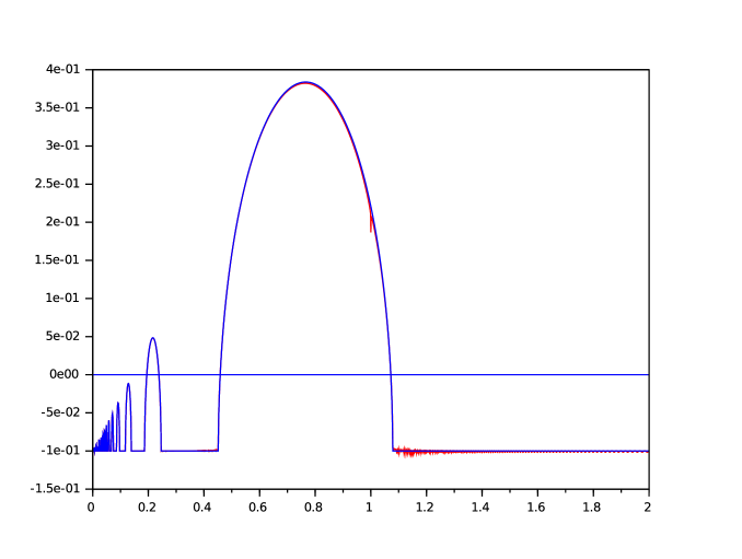
Figure 4 illustrates Proposition 4.1.

Refer to caption
Figure 4: In blue the general shape of ฯ‡dsuperscript๐œ’๐‘‘\chi^{d} for a=0.1๐‘Ž0.1a=0.1, b=2๐‘2b=2 and u=0.5๐‘ข0.5u=0.5. In red, x0subscript๐‘ฅ0x_{0} is in Eฮป2subscript๐ธsubscript๐œ†2E_{\lambda_{2}} for ฮฒ=1๐›ฝ1\beta=1.

5 A way to obtain several blow up areas

One of the expectations of this article was to get a planar linear switched system whose ฯ‡๐œ’\chi function admits several blow up areas. A quick look at the deterministic case (4) allowed us to believe that it could be possible with our system. Unfortunately the simulation we can see in Figure 2 seems to show that we did not manage to succeed. We slightly modify the jump times in order to mimic the deterministic evolution (15).

Let u=12๐‘ข12u=\frac{1}{2} (for sake of simplicity) and let n๐‘›n be a stricly positive integer. We now define the piecewise deterministic Markov process ((Xtn,Itn))tโ‰ฅ0subscriptsuperscriptsubscript๐‘‹๐‘ก๐‘›superscriptsubscript๐ผ๐‘ก๐‘›๐‘ก0((X_{t}^{n},I_{t}^{n}))_{t\geq 0} as follows: (It)tโฉพ0subscriptsubscript๐ผ๐‘ก๐‘ก0(I_{t})_{t\geqslant 0} is a continuous time Markov process defined on the state space {0,1,2,โ€ฆ,2โ€‹nโˆ’1}012โ€ฆ2๐‘›1\{0,1,2,...,2n-1\} with a constant jump rate nโ€‹ฮฒ2๐‘›๐›ฝ2\frac{n\beta}{2} and a jump mesure:

Q(i,.)=ฮดi+1ifi<2nโˆ’1,\displaystyle Q(i,.)=\delta_{i+1}\quad\text{if}\quad i<2n-1,
Q(2nโˆ’1,.)=ฮด0.\displaystyle Q(2n-1,.)=\delta_{0}.

And we define (Xtn)tโ‰ฅ0subscriptsuperscriptsubscript๐‘‹๐‘ก๐‘›๐‘ก0(X_{t}^{n})_{t\geq 0} as the solution of:

Xt=X0n+โˆซ0tA๐Ÿ™It<nโ€‹Xsnโ€‹๐‘‘s.subscript๐‘‹๐‘กsuperscriptsubscript๐‘‹0๐‘›superscriptsubscript0๐‘กsubscript๐ดsubscript1subscript๐ผ๐‘ก๐‘›superscriptsubscript๐‘‹๐‘ ๐‘›differential-d๐‘ X_{t}=X_{0}^{n}+\int_{0}^{t}A_{\mathds{1}_{I_{t}<n}}X_{s}^{n}ds.

This process looks like (1). The difference lies in the fact that, instead of waiting for an exponential time of parameter ฮฒ2๐›ฝ2\frac{\beta}{2} before jumping from a matrix to the other, the process waits for a time following a Gamma law of mean 2ฮฒ2๐›ฝ\frac{2}{\beta} and variance 4nโ€‹ฮฒ24๐‘›superscript๐›ฝ2\frac{4}{n\beta^{2}}.
The next result compares the stochastic process to the periodic one.
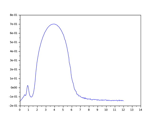
Refer to caption
Figure 5: For a=0.15๐‘Ž0.15a=0.15, b=3๐‘3b=3 and n=50๐‘›50n=50, a second blow up area appears in ฯ‡๐œ’\chi.
Lemma 5.1.

For every T>0๐‘‡0T>0, the process (Xtn)0โฉฝtโฉฝTsubscriptsuperscriptsubscript๐‘‹๐‘ก๐‘›0๐‘ก๐‘‡(X_{t}^{n})_{0\leqslant t\leqslant T} uniformly converges to the deterministic process (Xt)0โฉฝtโฉฝTsubscriptsubscript๐‘‹๐‘ก0๐‘ก๐‘‡(X_{t})_{0\leqslant t\leqslant T} solution of (15).

Proof.

Let us call Nnโ€‹(t)superscript๐‘๐‘›๐‘กN^{n}(t) the number of jumps before t๐‘กt of the process (Itn)superscriptsubscript๐ผ๐‘ก๐‘›(I_{t}^{n}), ฯ„1nsuperscriptsubscript๐œ1๐‘›\tau_{1}^{n}, ฯ„2nsuperscriptsubscript๐œ2๐‘›\tau_{2}^{n}, โ€ฆ,ฯ„Nโ€‹(t)nsuperscriptsubscript๐œ๐‘๐‘ก๐‘›\tau_{N(t)}^{n} are the interjump times, they follow a gamma law of mean 1ฮฒ1๐›ฝ\frac{1}{\beta} and variance 1nโ€‹ฮฒ21๐‘›superscript๐›ฝ2\frac{1}{n\beta^{2}}. We denote atn=tโˆ’โˆ‘k=1Nโ€‹(t)ฯ„knsuperscriptsubscript๐‘Ž๐‘ก๐‘›๐‘กsuperscriptsubscript๐‘˜1๐‘๐‘กsuperscriptsubscript๐œ๐‘˜๐‘›a_{t}^{n}=t-\sum_{k=1}^{N(t)}\tau_{k}^{n}. We finally call ฮพ1nsuperscriptsubscript๐œ‰1๐‘›\xi_{1}^{n}, ฮพ2nsuperscriptsubscript๐œ‰2๐‘›\xi_{2}^{n}, โ€ฆ,ฮพNโ€‹(t)+1nโˆˆ{0,1}superscriptsubscript๐œ‰๐‘๐‘ก1๐‘›01\xi_{N(t)+1}^{n}\in\{0,1\} the states.
By simply solving the equation for the process (Xtn)superscriptsubscript๐‘‹๐‘ก๐‘›(X_{t}^{n}) and calculating the matrices exponential we obtain:

Xtn=eโˆ’aโ€‹tโ€‹BฮพNnโ€‹(t)+1nโ€‹(atn)โ€‹BฮพNnโ€‹(t)nโ€‹(ฯ„Nnโ€‹(t)n)โ€‹โ‹ฏโ€‹Bฮพ1nโ€‹(ฯ„1n)superscriptsubscript๐‘‹๐‘ก๐‘›superscript๐‘’๐‘Ž๐‘กsubscript๐ตsuperscriptsubscript๐œ‰superscript๐‘๐‘›๐‘ก1๐‘›superscriptsubscript๐‘Ž๐‘ก๐‘›subscript๐ตsuperscriptsubscript๐œ‰superscript๐‘๐‘›๐‘ก๐‘›superscriptsubscript๐œsuperscript๐‘๐‘›๐‘ก๐‘›โ‹ฏsubscript๐ตsuperscriptsubscript๐œ‰1๐‘›superscriptsubscript๐œ1๐‘›X_{t}^{n}=e^{-at}B_{\xi_{N^{n}(t)+1}^{n}}(a_{t}^{n})B_{\xi_{N^{n}(t)}^{n}}(\tau_{N^{n}(t)}^{n})\cdots B_{\xi_{1}^{n}}(\tau_{1}^{n})

where

B0โ€‹(t)=(cosโก(t)bโ€‹sinโก(t)โˆ’1bโ€‹sinโก(t)cosโก(t))andB1โ€‹(t)=(cosโก(t)1bโ€‹sinโก(t)โˆ’bโ€‹sinโก(t)cosโก(t)).formulae-sequencesubscript๐ต0๐‘กmatrix๐‘ก๐‘๐‘ก1๐‘๐‘ก๐‘กandsubscript๐ต1๐‘กmatrix๐‘ก1๐‘๐‘ก๐‘๐‘ก๐‘กB_{0}(t)=\begin{pmatrix}\cos(t)&b\sin(t)\\ -\frac{1}{b}\sin(t)&\cos(t)\end{pmatrix}\quad\text{and}\quad B_{1}(t)=\begin{pmatrix}\cos(t)&\frac{1}{b}\sin(t)\\ -b\sin(t)&\cos(t)\end{pmatrix}.

Let us call Nโ€‹(t)๐‘๐‘กN(t) the number of jumps of the deterministic process. We have:

Xt=eโˆ’aโ€‹tโ€‹BฮพNโ€‹(t)+1โ€‹(at)โ€‹BฮพNโ€‹(t)โ€‹(1ฮฒ)โ€‹โ‹ฏโ€‹Bฮพ1โ€‹(1ฮฒ).subscript๐‘‹๐‘กsuperscript๐‘’๐‘Ž๐‘กsubscript๐ตsubscript๐œ‰๐‘๐‘ก1subscript๐‘Ž๐‘กsubscript๐ตsubscript๐œ‰๐‘๐‘ก1๐›ฝโ‹ฏsubscript๐ตsubscript๐œ‰11๐›ฝX_{t}=e^{-at}B_{\xi_{N(t)+1}}(a_{t})B_{\xi_{N(t)}}(\frac{1}{\beta})\cdots B_{\xi_{1}}(\frac{1}{\beta}).

We form the difference:

โ€–Xtnโˆ’Xtโ€–โฉฝnormsuperscriptsubscript๐‘‹๐‘ก๐‘›subscript๐‘‹๐‘ก\displaystyle\|X_{t}^{n}-X_{t}\|\leqslant\text{ } ๐Ÿ™Nnโ€‹(t)=Nโ€‹(t)โ€‹โ€–BฮพNโ€‹(t)+1nโ€‹(atn)โ€‹โ‹ฏโ€‹Bฮพ1nโ€‹(ฯ„1n)โˆ’BฮพNโ€‹(t)+1โ€‹(at)โ€‹โ‹ฏโ€‹Bฮพ1โ€‹(1ฮฒ)โ€–โ€‹โ€–X0โ€–subscript1superscript๐‘๐‘›๐‘ก๐‘๐‘กnormsubscript๐ตsuperscriptsubscript๐œ‰๐‘๐‘ก1๐‘›superscriptsubscript๐‘Ž๐‘ก๐‘›โ‹ฏsubscript๐ตsuperscriptsubscript๐œ‰1๐‘›superscriptsubscript๐œ1๐‘›subscript๐ตsubscript๐œ‰๐‘๐‘ก1subscript๐‘Ž๐‘กโ‹ฏsubscript๐ตsubscript๐œ‰11๐›ฝnormsubscript๐‘‹0\displaystyle\mathds{1}_{N^{n}(t)=N(t)}\|B_{\xi_{N(t)+1}^{n}}(a_{t}^{n})\cdots B_{\xi_{1}^{n}}(\tau_{1}^{n})-B_{\xi_{N(t)+1}}(a_{t})\cdots B_{\xi_{1}}(\frac{1}{\beta})\|\|X_{0}\|
+\displaystyle+ ๐Ÿ™Nnโ€‹(t)โ‰ Nโ€‹(t)โ€‹โ€–BฮพNnโ€‹(t)+1nโ€‹(atn)โ€‹โ‹ฏโ€‹Bฮพ1nโ€‹(ฯ„1n)โˆ’BฮพNโ€‹(t)+1โ€‹(at)โ€‹โ‹ฏโ€‹Bฮพ1โ€‹(1ฮฒ)โ€–โ€‹โ€–X0โ€–.subscript1superscript๐‘๐‘›๐‘ก๐‘๐‘กnormsubscript๐ตsuperscriptsubscript๐œ‰superscript๐‘๐‘›๐‘ก1๐‘›superscriptsubscript๐‘Ž๐‘ก๐‘›โ‹ฏsubscript๐ตsuperscriptsubscript๐œ‰1๐‘›superscriptsubscript๐œ1๐‘›subscript๐ตsubscript๐œ‰๐‘๐‘ก1subscript๐‘Ž๐‘กโ‹ฏsubscript๐ตsubscript๐œ‰11๐›ฝnormsubscript๐‘‹0\displaystyle\mathds{1}_{N^{n}(t)\neq N(t)}\|B_{\xi_{N^{n}(t)+1}^{n}}(a_{t}^{n})\cdots B_{\xi_{1}^{n}}(\tau_{1}^{n})-B_{\xi_{N(t)+1}}(a_{t})\cdots B_{\xi_{1}}(\frac{1}{\beta})\|\|X_{0}\|.

We can prove by induction on Nโ€‹(t)๐‘๐‘กN(t) that:

โ€–BฮพNโ€‹(t)+1nโ€‹(atn)โ€‹โ‹ฏโ€‹Bฮพ1nโ€‹(ฯ„1n)โˆ’BฮพNโ€‹(t)+1โ€‹(at)โ€‹โ‹ฏโ€‹Bฮพ1โ€‹(1ฮฒ)โ€–โŸถ0โ€‹ย in probability.โŸถnormsubscript๐ตsuperscriptsubscript๐œ‰๐‘๐‘ก1๐‘›superscriptsubscript๐‘Ž๐‘ก๐‘›โ‹ฏsubscript๐ตsuperscriptsubscript๐œ‰1๐‘›superscriptsubscript๐œ1๐‘›subscript๐ตsubscript๐œ‰๐‘๐‘ก1subscript๐‘Ž๐‘กโ‹ฏsubscript๐ตsubscript๐œ‰11๐›ฝ0ย in probability.\|B_{\xi_{N(t)+1}^{n}}(a_{t}^{n})\cdots B_{\xi_{1}^{n}}(\tau_{1}^{n})-B_{\xi_{N(t)+1}}(a_{t})\cdots B_{\xi_{1}}(\frac{1}{\beta})\|\longrightarrow 0\text{ in probability.}

The case Nโ€‹(t)=1๐‘๐‘ก1N(t)=1 shows us what happens:

โ€–Bฮพ2โ€‹(tโˆ’ฯ„1)โ€‹Bฮพ1โ€‹(ฯ„1)โˆ’Bฮพ2โ€‹(tโˆ’1ฮฒ)โ€‹Bฮพ1โ€‹(1ฮฒ)โ€–normsubscript๐ตsubscript๐œ‰2๐‘กsubscript๐œ1subscript๐ตsubscript๐œ‰1subscript๐œ1subscript๐ตsubscript๐œ‰2๐‘ก1๐›ฝsubscript๐ตsubscript๐œ‰11๐›ฝ\displaystyle\|B_{\xi_{2}}(t-\tau_{1})B_{\xi_{1}}(\tau_{1})-B_{\xi_{2}}(t-\frac{1}{\beta})B_{\xi_{1}}(\frac{1}{\beta})\| โฉฝโ€–Bฮพ2โ€‹(tโˆ’ฯ„1)โ€–โ€‹โ€–Bฮพ1โ€‹(ฯ„1)โˆ’Bฮพ1โ€‹(1ฮฒ)โ€–absentnormsubscript๐ตsubscript๐œ‰2๐‘กsubscript๐œ1normsubscript๐ตsubscript๐œ‰1subscript๐œ1subscript๐ตsubscript๐œ‰11๐›ฝ\displaystyle\leqslant\|B_{\xi_{2}}(t-\tau_{1})\|\|B_{\xi_{1}}(\tau_{1})-B_{\xi_{1}}(\frac{1}{\beta})\|
+โ€–Bฮพ2โ€‹(1ฮฒ)โˆ’Bฮพ2โ€‹(ฯ„2)โ€–โ€‹โ€–Bฮพ1โ€‹(ฯ„1)โ€–normsubscript๐ตsubscript๐œ‰21๐›ฝsubscript๐ตsubscript๐œ‰2subscript๐œ2normsubscript๐ตsubscript๐œ‰1subscript๐œ1\displaystyle\text{ }+\|B_{\xi_{2}}(\frac{1}{\beta})-B_{\xi_{2}}(\tau_{2})\|\|B_{\xi_{1}}(\tau_{1})\|
โฉฝC1โ€‹|ฯ„1โˆ’1ฮฒ|.absentsubscript๐ถ1subscript๐œ11๐›ฝ\displaystyle\leqslant C_{1}|\tau_{1}-\frac{1}{\beta}|.

By using the inequality of Bienaymรฉ-Tchebychev, we gain the claimed convergence. Moreover we can say that this convergence also holds in L1superscript๐ฟ1L^{1} as the random variable is bounded because our process does not explode in a finite time.
We prove now that โ„™โ€‹[Nnโ€‹(t)=Nโ€‹(t)]โŸถ1โŸถโ„™delimited-[]superscript๐‘๐‘›๐‘ก๐‘๐‘ก1\mathbb{P}[N^{n}(t)=N(t)]\longrightarrow 1 when n๐‘›n goes to +โˆž+\infty. First, let us write that Nโ€‹(t)=p๐‘๐‘ก๐‘N(t)=p and t=pฮฒ+ฮท๐‘ก๐‘๐›ฝ๐œ‚t=\frac{p}{\beta}+\eta where 0โฉฝฮท<1ฮฒ0๐œ‚1๐›ฝ0\leqslant\eta<\frac{1}{\beta}. We have:

โ„™โ€‹[Nnโ€‹(t)=p]โ„™delimited-[]superscript๐‘๐‘›๐‘ก๐‘\displaystyle\mathbb{P}[N^{n}(t)=p] =โ„™โ€‹[ฯ„1+ฯ„2+โ€ฆ+ฯ„pโฉฝt<ฯ„1+โ€ฆ+ฯ„p+ฯ„p+1]absentโ„™delimited-[]subscript๐œ1subscript๐œ2โ€ฆsubscript๐œ๐‘๐‘กsubscript๐œ1โ€ฆsubscript๐œ๐‘subscript๐œ๐‘1\displaystyle=\mathbb{P}\left[\tau_{1}+\tau_{2}+...+\tau_{p}\leqslant t<\tau_{1}+...+\tau_{p}+\tau_{p+1}\right]
=โ„™โ€‹[0โฉฝtโˆ’โˆ‘i=1pฯ„iโ€‹ย andย โ€‹t<โˆ‘i=1p+1ฯ„i]absentโ„™delimited-[]0๐‘กsuperscriptsubscript๐‘–1๐‘subscript๐œ๐‘–ย andย ๐‘กsuperscriptsubscript๐‘–1๐‘1subscript๐œ๐‘–\displaystyle=\mathbb{P}\left[0\leqslant t-\sum_{i=1}^{p}\tau_{i}\text{ and }t<\sum_{i=1}^{p+1}\tau_{i}\right]
=โ„™โ€‹[โˆ‘i=1pฯ„iโˆ’pฮฒ<ฮท]โ€‹โ„™โ€‹[tโ€‹<โˆ‘i=1p+1ฯ„iโ€‹ย |โ€‹ย โ€‹0โฉฝtโˆ’โˆ‘i=1pฯ„i].absentโ„™delimited-[]superscriptsubscript๐‘–1๐‘subscript๐œ๐‘–๐‘๐›ฝ๐œ‚โ„™delimited-[]๐‘กbrasuperscriptsubscript๐‘–1๐‘1subscript๐œ๐‘–ย ย 0๐‘กsuperscriptsubscript๐‘–1๐‘subscript๐œ๐‘–\displaystyle=\mathbb{P}\left[\sum_{i=1}^{p}\tau_{i}-\frac{p}{\beta}<\eta\right]\mathbb{P}\left[t<\sum_{i=1}^{p+1}\tau_{i}\text{ }|\text{ }0\leqslant t-\sum_{i=1}^{p}\tau_{i}\right].

The first probability goes to 111 when n๐‘›n goes to +โˆž+\infty thanks to the Bienaymรฉ-Tchebychev inequality and the other probability is nonzero. This means that we have the claimed convergence: โ„™โ€‹[Nnโ€‹(t)=Nโ€‹(t)]โŸถ1โŸถโ„™delimited-[]superscript๐‘๐‘›๐‘ก๐‘๐‘ก1\mathbb{P}[N^{n}(t)=N(t)]\longrightarrow 1 when n๐‘›n goes to +โˆž+\infty.
Back in the inequality, we take the expectation and using the previous results we prove that ๐”ผโ€‹[โ€–Xtnโˆ’Xtโ€–]๐”ผdelimited-[]normsuperscriptsubscript๐‘‹๐‘ก๐‘›subscript๐‘‹๐‘ก\mathbb{E}[\|X_{t}^{n}-X_{t}\|] goes to 00 uniformly on [0,T]0๐‘‡[0,T].
โˆŽ

6 Behaviour of the switched system with two centers of attraction

We slightly modify our initial system by shifting the centers of attraction of each flow. Assume that A0subscript๐ด0A_{0} and A1subscript๐ด1A_{1} are Hurwitz matrices and b0subscript๐‘0b_{0} and b1subscript๐‘1b_{1} in โ„dsuperscriptโ„๐‘‘\mathbb{R}^{d} (with b0โ‰ b1subscript๐‘0subscript๐‘1b_{0}\neq b_{1}). For i=0,1๐‘–01i=0,1 and xโˆˆโ„d๐‘ฅsuperscriptโ„๐‘‘x\in\mathbb{R}^{d}, let t>0โ†ฆฯ†tiโ€‹(x)๐‘ก0maps-tosuperscriptsubscript๐œ‘๐‘ก๐‘–๐‘ฅt>0\mapsto\varphi_{t}^{i}(x) the solution of xห™t=Aiโ€‹(xtโˆ’bi)subscriptห™๐‘ฅ๐‘กsubscript๐ด๐‘–subscript๐‘ฅ๐‘กsubscript๐‘๐‘–\dot{x}_{t}=A_{i}(x_{t}-b_{i}) with x0=xsubscript๐‘ฅ0๐‘ฅx_{0}=x.

Remark 6.1.

There exists Cโฉพ1๐ถ1C\geqslant 1 and ฮท>0๐œ‚0\eta>0 such that, for all tโฉพ0๐‘ก0t\geqslant 0,

โ€–ฯ†tiโ€‹(x)โˆ’biโ€–โฉฝCโ€‹eโˆ’ฮทโ€‹tโ€‹โ€–xโˆ’biโ€–.normsuperscriptsubscript๐œ‘๐‘ก๐‘–๐‘ฅsubscript๐‘๐‘–๐ถsuperscript๐‘’๐œ‚๐‘กnorm๐‘ฅsubscript๐‘๐‘–{{\left\|\varphi_{t}^{i}(x)-b_{i}\right\|}}\leqslant Ce^{-\eta t}{{\left\|x-b_{i}\right\|}}.

The goal of this section is to discuss the long time behavior of (Xt)subscript๐‘‹๐‘ก(X_{t}) if (It)tโฉพ0subscriptsubscript๐ผ๐‘ก๐‘ก0{(I_{t})}_{t\geqslant 0} jumps from 1 to 0 (resp. from 0 to 1) with rate ฮป1subscript๐œ†1\lambda_{1} (resp. ฮป0subscript๐œ†0\lambda_{0}) i.e. (Xt)subscript๐‘‹๐‘ก(X_{t}) solution of (2).
Let us couple two paths (Xt,It)subscript๐‘‹๐‘กsubscript๐ผ๐‘ก(X_{t},I_{t}) and (X~t,I~t)subscript~๐‘‹๐‘กsubscript~๐ผ๐‘ก(\tilde{X}_{t},\tilde{I}_{t}) starting from (x,i)๐‘ฅ๐‘–(x,i) and (x~,i)~๐‘ฅ๐‘–(\tilde{x},i) choosing the same jump times i.e. the same process (It)tโฉพ0subscriptsubscript๐ผ๐‘ก๐‘ก0{(I_{t})}_{t\geqslant 0}. Then, the difference Dt=Xtโˆ’X~tsubscript๐ท๐‘กsubscript๐‘‹๐‘กsubscript~๐‘‹๐‘กD_{t}=X_{t}-\tilde{X}_{t} is solution of Dห™t=AItโ€‹Dtsubscriptห™๐ท๐‘กsubscript๐ดsubscript๐ผ๐‘กsubscript๐ท๐‘ก\dot{D}_{t}=A_{I_{t}}D_{t}.

Remark 6.2.

If the initial discrete components are different, one has to wait for a random time T๐‘‡T following an exponential law of parameter ฮป0+ฮป1subscript๐œ†0subscript๐œ†1\lambda_{0}+\lambda_{1} and then, they can be chosen equal for all tโฉพT๐‘ก๐‘‡t\geqslant T.

One can write Dt=Rtโ€‹Utsubscript๐ท๐‘กsubscript๐‘…๐‘กsubscript๐‘ˆ๐‘กD_{t}=R_{t}U_{t} with Rt>0subscript๐‘…๐‘ก0R_{t}>0 and UtโˆˆS1subscript๐‘ˆ๐‘กsuperscript๐‘†1U_{t}\in S^{1}. Recall that

Rt=R0โ€‹expโก(โˆซ0t๐’œโ€‹(Us,Is)โ€‹๐‘‘s).subscript๐‘…๐‘กsubscript๐‘…0superscriptsubscript0๐‘ก๐’œsubscript๐‘ˆ๐‘ subscript๐ผ๐‘ differential-d๐‘ R_{t}=R_{0}\exp{{\left(\int_{0}^{t}\mathcal{A}(U_{s},I_{s})ds\right)}}.

Let us define

ฮจpโ€‹(t)=supuโˆˆS1,i=0,1[๐”ผ(u,i)โ€‹(expโก(pโ€‹โˆซ0t๐’œโ€‹(Us,Is)โ€‹๐‘‘s))]1/p.subscriptฮจ๐‘๐‘กsubscriptsupremumformulae-sequence๐‘ขsuperscript๐‘†1๐‘–01superscriptdelimited-[]subscript๐”ผ๐‘ข๐‘–๐‘superscriptsubscript0๐‘ก๐’œsubscript๐‘ˆ๐‘ subscript๐ผ๐‘ differential-d๐‘ 1๐‘\Psi_{p}(t)=\sup_{u\in S^{1},i=0,1}{{\left[\mathbb{E}_{(u,i)}{{\left(\exp{{\left(p\int_{0}^{t}\mathcal{A}(U_{s},I_{s})ds\right)}}\right)}}\right]}}^{1/p}.

Thanks to Markov property, the function ฮจpsubscriptฮจ๐‘\Psi_{p} satisfies ฮจpโ€‹(t+s)โฉฝฮจpโ€‹(t)โ€‹ฮจpโ€‹(s)subscriptฮจ๐‘๐‘ก๐‘ subscriptฮจ๐‘๐‘กsubscriptฮจ๐‘๐‘ \Psi_{p}(t+s)\leqslant\Psi_{p}(t)\Psi_{p}(s). As a consequence, there exists ฯ‡psubscript๐œ’๐‘\chi_{p} such that

ฯ‡p=limtโ†’โˆž1tโ€‹logโกฮจpโ€‹(t).subscript๐œ’๐‘subscriptโ†’๐‘ก1๐‘กsubscriptฮจ๐‘๐‘ก\chi_{p}=\lim_{t\to\infty}\frac{1}{t}\log\Psi_{p}(t).

Moreover, Jensenโ€™s inequality ensures that ฯ‡pโฉพฯ‡subscript๐œ’๐‘๐œ’\chi_{p}\geqslant\chi. As a consequence, it is possible that Xtโ†’0โ†’subscript๐‘‹๐‘ก0X_{t}\to 0 a.s. with ฯ‡p>0subscript๐œ’๐‘0\chi_{p}>0 for some p>0๐‘0p>0.

Remark 6.3.

It is not easy to determine the sign of the Lyapunov exponent ฯ‡psubscript๐œ’๐‘\chi_{p}.

Lemma 6.4.

When ฮป0subscript๐œ†0\lambda_{0}, ฮป1subscript๐œ†1\lambda_{1} and p๐‘p are sufficiently small, there is convergence in Wasserstein distance for (Dt)subscript๐ท๐‘ก(D_{t}) after the coupling of the discrete components.

Proof.

Once again, we assume that the initial discrete components are equal. Denote by Ntsubscript๐‘๐‘กN_{t} the number of jumps for (It)tโฉพ0subscriptsubscript๐ผ๐‘ก๐‘ก0{(I_{t})}_{t\geqslant 0} before time t๐‘กt. One has It=(โˆ’1)Ntโ€‹I0subscript๐ผ๐‘กsuperscript1subscript๐‘๐‘กsubscript๐ผ0I_{t}=(-1)^{N_{t}}I_{0}.

Dt=expโก((tโˆ’TNt)โ€‹ATNt)โ€‹expโก((TNtโˆ’TNtโˆ’1)โ€‹AINtโˆ’1)โ€‹โ‹ฏโ€‹expโก((T2โˆ’T1)โ€‹AIT1)โ€‹expโก(T1โ€‹AI0)โ€‹D0.subscript๐ท๐‘ก๐‘กsubscript๐‘‡subscript๐‘๐‘กsubscript๐ดsubscript๐‘‡subscript๐‘๐‘กsubscript๐‘‡subscript๐‘๐‘กsubscript๐‘‡subscript๐‘๐‘ก1subscript๐ดsubscript๐ผsubscript๐‘๐‘ก1โ‹ฏsubscript๐‘‡2subscript๐‘‡1subscript๐ดsubscript๐ผsubscript๐‘‡1subscript๐‘‡1subscript๐ดsubscript๐ผ0subscript๐ท0D_{t}=\exp{{\left((t-T_{N_{t}})A_{T_{N_{t}}}\right)}}\exp{{\left((T_{N_{t}}-T_{N_{t}-1})A_{I_{N_{t}-1}}\right)}}\cdots\exp{{\left((T_{2}-T_{1})A_{I_{T_{1}}}\right)}}\exp{{\left(T_{1}A_{I_{0}}\right)}}D_{0}.

Using Remarkย 6.1, one has

โ€–Dtโ€–โฉฝCNt+1โ€‹eโˆ’ฮทโ€‹tโ€‹โ€–D0โ€–.normsubscript๐ท๐‘กsuperscript๐ถsubscript๐‘๐‘ก1superscript๐‘’๐œ‚๐‘กnormsubscript๐ท0{{\left\|D_{t}\right\|}}\leqslant C^{N_{t}+1}e^{-\eta t}{{\left\|D_{0}\right\|}}.

If the jump rates of I๐ผI are equal, (ฮป0=ฮป1=ฮป)\lambda_{0}=\lambda_{1}=\lambda), then (Nt)tโฉพ0subscriptsubscript๐‘๐‘ก๐‘ก0{(N_{t})}_{t\geqslant 0} is a simple Poisson process and

[๐”ผโ€‹(โ€–Dtโ€–p)]1/pโฉฝCโ€‹expโก(โˆ’(ฮทโˆ’ฮปโ€‹(Cpโˆ’1)p)โ€‹t)โ€‹[๐”ผโ€‹(โ€–D0โ€–p)]1/p.superscriptdelimited-[]๐”ผsuperscriptnormsubscript๐ท๐‘ก๐‘1๐‘๐ถ๐œ‚๐œ†superscript๐ถ๐‘1๐‘๐‘กsuperscriptdelimited-[]๐”ผsuperscriptnormsubscript๐ท0๐‘1๐‘{{\left[\mathbb{E}{{\left({{\left\|D_{t}\right\|}}^{p}\right)}}\right]}}^{1/p}\leqslant C\exp{{\left(-{{\left(\eta-\frac{\lambda(C^{p}-1)}{p}\right)}}t\right)}}{{\left[\mathbb{E}{{\left({{\left\|D_{0}\right\|}}^{p}\right)}}\right]}}^{1/p}.

This ensures that when ฮป๐œ†\lambda and p๐‘p are sufficiently small one can establish convergence in Wasserstein distance, after the coupling of the discrete components (see [4]).

If the jump rates are not equal, (Nt)tโฉพ0subscriptsubscript๐‘๐‘ก๐‘ก0{(N_{t})}_{t\geqslant 0} is not a Poisson process. For a fixed cโˆˆโ„๐‘โ„c\in\mathbb{R}, let us define Giโ€‹(t)=๐”ผiโ€‹(cNt)subscript๐บ๐‘–๐‘กsubscript๐”ผ๐‘–superscript๐‘subscript๐‘๐‘กG_{i}(t)=\mathbb{E}_{i}(c^{N_{t}}). Then, if T๐‘‡T is the first jump time,

G1โ€‹(t)subscript๐บ1๐‘ก\displaystyle G_{1}(t) =๐”ผ1โ€‹(cNtโ€‹๐Ÿ™{Tโฉฝt})+๐”ผ1โ€‹(cNtโ€‹๐Ÿ™{T>t})absentsubscript๐”ผ1superscript๐‘subscript๐‘๐‘กsubscript1๐‘‡๐‘กsubscript๐”ผ1superscript๐‘subscript๐‘๐‘กsubscript1๐‘‡๐‘ก\displaystyle=\mathbb{E}_{1}{{\left(c^{N_{t}}\mathds{1}_{{\left\{T\leqslant t\right\}}}\right)}}+\mathbb{E}_{1}{{\left(c^{N_{t}}\mathds{1}_{{\left\{T>t\right\}}}\right)}}
=โˆซ0tcโ€‹G0โ€‹(tโˆ’s)โ€‹ฮป1โ€‹eโˆ’ฮป1โ€‹sโ€‹๐‘‘s+eโˆ’ฮป1โ€‹t.absentsuperscriptsubscript0๐‘ก๐‘subscript๐บ0๐‘ก๐‘ subscript๐œ†1superscript๐‘’subscript๐œ†1๐‘ differential-d๐‘ superscript๐‘’subscript๐œ†1๐‘ก\displaystyle=\int_{0}^{t}cG_{0}(t-s)\lambda_{1}e^{-\lambda_{1}s}ds+e^{-\lambda_{1}t}.

As a consequence, thanks to an integration by parts,

G1โ€ฒโ€‹(t)superscriptsubscript๐บ1โ€ฒ๐‘ก\displaystyle G_{1}^{\prime}(t) =cโ€‹G0โ€‹(0)โ€‹ฮป1โ€‹eโˆ’ฮป1โ€‹t+cโ€‹โˆซ0tG0โ€ฒโ€‹(tโˆ’s)โ€‹ฮป1โ€‹eโˆ’ฮป1โ€‹sโ€‹๐‘‘sโˆ’ฮป1โ€‹eโˆ’ฮป1โ€‹tabsent๐‘subscript๐บ00subscript๐œ†1superscript๐‘’subscript๐œ†1๐‘ก๐‘superscriptsubscript0๐‘กsuperscriptsubscript๐บ0โ€ฒ๐‘ก๐‘ subscript๐œ†1superscript๐‘’subscript๐œ†1๐‘ differential-d๐‘ subscript๐œ†1superscript๐‘’subscript๐œ†1๐‘ก\displaystyle=cG_{0}(0)\lambda_{1}e^{-\lambda_{1}t}+c\int_{0}^{t}G_{0}^{\prime}(t-s)\lambda_{1}e^{-\lambda_{1}s}ds-\lambda_{1}e^{-\lambda_{1}t}
=cโ€‹ฮป1โ€‹eโˆ’ฮป1โ€‹t+cโ€‹[โˆ’G0โ€‹(tโˆ’s)โ€‹ฮป1โ€‹eโˆ’ฮป1โ€‹t]0tโˆ’cโ€‹โˆซ0tG0โ€‹(tโˆ’s)โ€‹ฮป12โ€‹eโˆ’ฮป1โ€‹sโ€‹๐‘‘sโˆ’ฮป1โ€‹eโˆ’ฮป1โ€‹tabsent๐‘subscript๐œ†1superscript๐‘’subscript๐œ†1๐‘ก๐‘superscriptsubscriptdelimited-[]subscript๐บ0๐‘ก๐‘ subscript๐œ†1superscript๐‘’subscript๐œ†1๐‘ก0๐‘ก๐‘superscriptsubscript0๐‘กsubscript๐บ0๐‘ก๐‘ superscriptsubscript๐œ†12superscript๐‘’subscript๐œ†1๐‘ differential-d๐‘ subscript๐œ†1superscript๐‘’subscript๐œ†1๐‘ก\displaystyle=c\lambda_{1}e^{-\lambda_{1}t}+c{{\left[-G_{0}(t-s)\lambda_{1}e^{-\lambda_{1}t}\right]}}_{0}^{t}-c\int_{0}^{t}G_{0}(t-s)\lambda_{1}^{2}e^{-\lambda_{1}s}ds-\lambda_{1}e^{-\lambda_{1}t}
=โˆ’ฮป1โ€‹G1โ€‹(t)+ฮป1โ€‹cโ€‹G0โ€‹(t).absentsubscript๐œ†1subscript๐บ1๐‘กsubscript๐œ†1๐‘subscript๐บ0๐‘ก\displaystyle=-\lambda_{1}G_{1}(t)+\lambda_{1}cG_{0}(t).

Notice that, if ฮป1=ฮป0subscript๐œ†1subscript๐œ†0\lambda_{1}=\lambda_{0}, one recovers that G0โ€‹(t)=G1โ€‹(t)=expโก(ฮปโ€‹tโ€‹(cโˆ’1))subscript๐บ0๐‘กsubscript๐บ1๐‘ก๐œ†๐‘ก๐‘1G_{0}(t)=G_{1}(t)=\exp(\lambda t(c-1)). In the general case, G0subscript๐บ0G_{0} and G1subscript๐บ1G_{1} are solutions of

yโ€ฒโ€ฒ+(ฮป0+ฮป1)โ€‹yโ€ฒ+ฮป0โ€‹ฮป1โ€‹(1โˆ’c2)โ€‹y=0superscript๐‘ฆโ€ฒโ€ฒsubscript๐œ†0subscript๐œ†1superscript๐‘ฆโ€ฒsubscript๐œ†0subscript๐œ†11superscript๐‘2๐‘ฆ0y^{\prime\prime}+(\lambda_{0}+\lambda_{1})y^{\prime}+\lambda_{0}\lambda_{1}(1-c^{2})y=0

with respective initial conditions Giโ€‹(0)=1subscript๐บ๐‘–01G_{i}(0)=1, Giโ€ฒโ€‹(0)=ฮปiโ€‹(cโˆ’1)superscriptsubscript๐บ๐‘–โ€ฒ0subscript๐œ†๐‘–๐‘1G_{i}^{\prime}(0)=\lambda_{i}(c-1).

After solving this simple equation, it also comes that for ฮป๐œ†\lambda and p๐‘p small enough, we can establish convergence in Wasserstein distance. โˆŽ

We are now interested in the invariant measure, if it exists, of our process (Xt)tโฉพ0subscriptsubscript๐‘‹๐‘ก๐‘ก0(X_{t})_{t\geqslant 0} solution of (2). Let us call T0=0subscript๐‘‡00T_{0}=0, T1subscript๐‘‡1T_{1}, โ€ฆ, Tnsubscript๐‘‡๐‘›T_{n} the jumping times of the process (Xt)subscript๐‘‹๐‘ก(X_{t}) and ฯ„0subscript๐œ0\tau_{0}, ฯ„1subscript๐œ1\tau_{1}, โ€ฆ, ฯ„nsubscript๐œ๐‘›\tau_{n}, the interjump times following an exponential law of parameters ฮป0subscript๐œ†0\lambda_{0} and ฮป1subscript๐œ†1\lambda_{1} alternatively. Let us define Yn=XT2โ€‹nsubscript๐‘Œ๐‘›subscript๐‘‹subscript๐‘‡2๐‘›Y_{n}=X_{T_{2n}}. By simply solving the equation 2 between each jumping times we obtain:

Yn=eฯ„n+1โ€‹A1โ€‹eฯ„nโ€‹A0โ€‹Ynโˆ’1โˆ’eฯ„n+1โ€‹b0+b1.subscript๐‘Œ๐‘›superscript๐‘’subscript๐œ๐‘›1subscript๐ด1superscript๐‘’subscript๐œ๐‘›subscript๐ด0subscript๐‘Œ๐‘›1superscript๐‘’subscript๐œ๐‘›1subscript๐‘0subscript๐‘1Y_{n}=e^{\tau_{n+1}A_{1}}e^{\tau_{n}A_{0}}Y_{n-1}-e^{\tau_{n+1}}b_{0}+b_{1}.

Applying Kestenโ€™s renewal theorem ([11]) to the discrete process (Yn)subscript๐‘Œ๐‘›(Y_{n}) will give some informations about the tail of the invariant measure of (Xt)subscript๐‘‹๐‘ก(X_{t}).

Theorem 6.5.

If there is no deterministic control that makes the deterministic process associated to (Yt(Y_{t}) explodes, it means that there exists an invariant measure ฮผ๐œ‡\mu for our process and the support of ฮผ๐œ‡\mu is necessarily bounded.

In the other hand, we assume that ฯ‡<0๐œ’0\chi<0 and that there exists a deterministic control such as:

โˆƒkโˆˆ2โ€‹โ„•+1โ€‹ย such asย โ€‹โˆ€xโˆˆ๐•Šdโˆ’1,โˆƒt0,t1,โ€ฆ,tk>0โ€‹ย such asย โ€‹โ€–etkโ€‹AIkโ€‹โ€ฆโ€‹et1โ€‹AI1โ€‹et0โ€‹AI0โ€‹xโ€–>โ€–xโ€–.formulae-sequence๐‘˜2โ„•1ย such asย for-all๐‘ฅsubscript๐•Š๐‘‘1subscript๐‘ก0subscript๐‘ก1โ€ฆsubscript๐‘ก๐‘˜0ย such asย normsuperscript๐‘’subscript๐‘ก๐‘˜subscript๐ดsubscript๐ผ๐‘˜โ€ฆsuperscript๐‘’subscript๐‘ก1subscript๐ดsubscript๐ผ1superscript๐‘’subscript๐‘ก0subscript๐ดsubscript๐ผ0๐‘ฅnorm๐‘ฅ\exists k\in 2\mathbb{N}+1\text{ such as }\forall x\in\mathbb{S}_{d-1},\exists t_{0},t_{1},...,t_{k}>0\text{ such as }\|e^{t_{k}A_{I_{k}}}...e^{t_{1}A_{I_{1}}}e^{t_{0}A_{I_{0}}}x\|>\|x\|. (16)

We call B=eฯ„kโ€‹AIkโ€‹โ€ฆโ€‹eฯ„1โ€‹AI1โ€‹eฯ„0โ€‹AI0๐ตsuperscript๐‘’subscript๐œ๐‘˜subscript๐ดsubscript๐ผ๐‘˜โ€ฆsuperscript๐‘’subscript๐œ1subscript๐ดsubscript๐ผ1superscript๐‘’subscript๐œ0subscript๐ดsubscript๐ผ0B=e^{\tau_{k}A_{I_{k}}}...e^{\tau_{1}A_{I_{1}}}e^{\tau_{0}A_{I_{0}}} and B0subscript๐ต0B_{0}, B1subscript๐ต1B_{1}, โ€ฆ, Bnsubscript๐ต๐‘›B_{n} n๐‘›n random variables i.i.d following the law of B๐ตB. We also assume that:

maxnโฉพ0โ€‹ย โ€‹โ„™โ€‹(Bnโ€‹โ€ฆโ€‹B0โ€‹xโ€–Bnโ€‹โ€ฆโ€‹B0โ€‹xโ€–โˆˆU)>0โ€‹ย for allย โ€‹xโˆˆ๐•Šdโˆ’1โ€‹ย and any openย โ€‹โˆ…โ‰ UโŠ‚๐•Šdโˆ’1.๐‘›0ย โ„™subscript๐ต๐‘›โ€ฆsubscript๐ต0๐‘ฅnormsubscript๐ต๐‘›โ€ฆsubscript๐ต0๐‘ฅ๐‘ˆ0ย for allย ๐‘ฅsubscript๐•Š๐‘‘1ย and any openย ๐‘ˆsubscript๐•Š๐‘‘1\underset{n\geqslant 0}{\max}\text{ }\mathbb{P}\left(\frac{B_{n}...B_{0}x}{\|B_{n}...B_{0}x\|}\in U\right)>0\text{ for all }x\in\mathbb{S}_{d-1}\text{ and any open }\emptyset\neq U\subset\mathbb{S}_{d-1}. (17)
โ„™(Bn0โ€ฆB0โˆˆ.)โฉพฮณ0๐Ÿ™Bcโ€‹(ฮ“0)ฮปย for someย ฮ“0โˆˆGLd(โ„),ย n0โˆˆโ„•ย andย c,ฮณ0>0.\mathbb{P}(B_{n_{0}}...B_{0}\in.)\geqslant\gamma_{0}\mathds{1}_{B_{c}(\Gamma_{0})}\lambda\text{ for some }\Gamma_{0}\in GL_{d}(\mathbb{R}),\text{ }n_{0}\in\mathbb{N}\text{ and }c,\gamma_{0}>0. (18)

where ฮป๐œ†\lambda is the Lebesgue measure on โ„n2superscriptโ„superscript๐‘›2\mathbb{R}^{n^{2}}. Under these assumptions, there exists a unique invariant measure ฮผ๐œ‡\mu for the process (Yt)subscript๐‘Œ๐‘ก(Y_{t}) and it has an heavy tail:

โˆƒp1>0โ€‹ย such asย โ€‹โˆ€0โฉฝp<p1๐”ผฮผโ€‹[โ€–Yโ€–p]โ€‹<+โˆžโ€‹ย andย โ€‹โˆ€p>โ€‹p1๐”ผฮผโ€‹[โ€–Yโ€–p]=+โˆž.formulae-sequencesubscript๐‘10ย such asย for-all0๐‘subscript๐‘1subscript๐”ผ๐œ‡delimited-[]superscriptnorm๐‘Œ๐‘expectationย andย for-all๐‘subscript๐‘1subscript๐”ผ๐œ‡delimited-[]superscriptnorm๐‘Œ๐‘\exists p_{1}>0\text{ such as }\forall 0\leqslant p<p_{1}\quad\mathbb{E}_{\mu}[\|Y\|^{p}]<+\infty\text{ and }\forall p>p_{1}\quad\mathbb{E}_{\mu}[\|Y\|^{p}]=+\infty.
Proof.

Let xโˆˆ๐•Šdโˆ’1๐‘ฅsubscript๐•Š๐‘‘1x\in\mathbb{S}_{d-1}. There exist t0subscript๐‘ก0t_{0}, t1subscript๐‘ก1t_{1},โ€ฆ ,tk>0subscript๐‘ก๐‘˜0t_{k}>0 such as:

โ€–etkโ€‹AIkโ€‹โ€ฆโ€‹et1โ€‹AI1โ€‹et0โ€‹AI0โ€‹xโ€–>โ€–xโ€–.normsuperscript๐‘’subscript๐‘ก๐‘˜subscript๐ดsubscript๐ผ๐‘˜โ€ฆsuperscript๐‘’subscript๐‘ก1subscript๐ดsubscript๐ผ1superscript๐‘’subscript๐‘ก0subscript๐ดsubscript๐ผ0๐‘ฅnorm๐‘ฅ\|e^{t_{k}A_{I_{k}}}...e^{t_{1}A_{I_{1}}}e^{t_{0}A_{I_{0}}}x\|>\|x\|.

Consequently, by continuity, there exist ฯต>0italic-ฯต0\epsilon>0 and ฮด>0๐›ฟ0\delta>0 such as:

โˆ€siโˆˆJi=(tiโˆ’ฮด,ti+ฮด),โ€–eskโ€‹AIkโ€‹โ€ฆโ€‹es1โ€‹A1โ€‹es0โ€‹A0โ€–โฉพ1+ฯต.formulae-sequencefor-allsubscript๐‘ ๐‘–subscript๐ฝ๐‘–subscript๐‘ก๐‘–๐›ฟsubscript๐‘ก๐‘–๐›ฟnormsuperscript๐‘’subscript๐‘ ๐‘˜subscript๐ดsubscript๐ผ๐‘˜โ€ฆsuperscript๐‘’subscript๐‘ 1subscript๐ด1superscript๐‘’subscript๐‘ 0subscript๐ด01italic-ฯต\forall s_{i}\in J_{i}=(t_{i}-\delta,t_{i}+\delta),\quad\|e^{s_{k}A_{I_{k}}}...e^{s_{1}A_{1}}e^{s_{0}A_{0}}\|\geqslant 1+\epsilon.

Let us write B=eฯ„kโ€‹AIkโ€‹โ€ฆโ€‹eฯ„1โ€‹A1โ€‹eฯ„0โ€‹A0๐ตsuperscript๐‘’subscript๐œ๐‘˜subscript๐ดsubscript๐ผ๐‘˜โ€ฆsuperscript๐‘’subscript๐œ1subscript๐ด1superscript๐‘’subscript๐œ0subscript๐ด0B=e^{\tau_{k}A_{I_{k}}}...e^{\tau_{1}A_{1}}e^{\tau_{0}A_{0}}, where ฯ„0subscript๐œ0\tau_{0}, ฯ„1subscript๐œ1\tau_{1},โ€ฆ ,ฯ„ksubscript๐œ๐‘˜\tau_{k} are k+1๐‘˜1k+1 random exponential variables. We have:

๐”ผโ€‹[โ€–Bโ€–p]๐”ผdelimited-[]superscriptnorm๐ต๐‘\displaystyle\mathbb{E}\left[\|B\|^{p}\right] โฉพ๐”ผโ€‹[๐Ÿ™ฯ„kโˆˆJkโ€‹โ€ฆโ€‹๐Ÿ™ฯ„1โˆˆJ1โ€‹๐Ÿ™ฯ„0โˆˆJ0โ€‹โ€–Bโ€–p]absent๐”ผdelimited-[]subscript1subscript๐œ๐‘˜subscript๐ฝ๐‘˜โ€ฆsubscript1subscript๐œ1subscript๐ฝ1subscript1subscript๐œ0subscript๐ฝ0superscriptnorm๐ต๐‘\displaystyle\geqslant\mathbb{E}\left[\mathds{1}_{\tau_{k}\in J_{k}}...\mathds{1}_{\tau_{1}\in J_{1}}\mathds{1}_{\tau_{0}\in J_{0}}\|B\|^{p}\right]
โฉพโ„™โ€‹(ฯ„kโˆˆJk)โ€‹โ€ฆโ€‹โ„™โ€‹(ฯ„1โˆˆJ1)โ€‹โ„™โ€‹(ฯ„0โˆˆJ0)โ€‹(1+ฯต)pabsentโ„™subscript๐œ๐‘˜subscript๐ฝ๐‘˜โ€ฆโ„™subscript๐œ1subscript๐ฝ1โ„™subscript๐œ0subscript๐ฝ0superscript1italic-ฯต๐‘\displaystyle\geqslant\mathbb{P}(\tau_{k}\in J_{k})...\mathbb{P}(\tau_{1}\in J_{1})\mathbb{P}(\tau_{0}\in J_{0})(1+\epsilon)^{p}

As ฯ„0subscript๐œ0\tau_{0}, ฯ„1subscript๐œ1\tau_{1},โ€ฆ ,ฯ„ksubscript๐œ๐‘˜\tau_{k} are k+1๐‘˜1k+1 exponential random variables, โ„™โ€‹(ฯ„kโˆˆJk)โ€‹โ€ฆโ€‹โ„™โ€‹(ฯ„1โˆˆJ1)โ€‹โ„™โ€‹(ฯ„0โˆˆJ0)>0โ„™subscript๐œ๐‘˜subscript๐ฝ๐‘˜โ€ฆโ„™subscript๐œ1subscript๐ฝ1โ„™subscript๐œ0subscript๐ฝ00\mathbb{P}(\tau_{k}\in J_{k})...\mathbb{P}(\tau_{1}\in J_{1})\mathbb{P}(\tau_{0}\in J_{0})>0. Consequently:

๐”ผโ€‹[โ€–Bโ€–p]โ€‹โŸถpโ†’+โˆž+โˆž,๐”ผdelimited-[]superscriptnorm๐ต๐‘โ†’๐‘โŸถ\mathbb{E}\left[\|B\|^{p}\right]\underset{p\rightarrow+\infty}{\longrightarrow}+\infty,

meaning that there exists x1>0subscript๐‘ฅ10x_{1}>0 such as ๐”ผโ€‹[โ€–Bโ€–x1]=1๐”ผdelimited-[]superscriptnorm๐ตsubscript๐‘ฅ11\mathbb{E}\left[\|B\|^{x_{1}}\right]=1. Consequently, if the process (Yt)subscript๐‘Œ๐‘ก(Y_{t}) does not explode, [1] ensures that under the invariant measure ฮผ๐œ‡\mu:

โ„™โ€‹(โ€–Yโ€–>r)โˆผcrx1.similar-toโ„™norm๐‘Œ๐‘Ÿ๐‘superscript๐‘Ÿsubscript๐‘ฅ1\mathbb{P}(\|Y\|>r)\sim\frac{c}{r^{x_{1}}}.

It implies that ฮผ๐œ‡\mu has finite moments of order p<x1๐‘subscript๐‘ฅ1p<x_{1}. โˆŽ

Remark 6.6.

In dimension 2, hypothesis (16) can be verified using the criteria in [3] which gives the existence of an explosive control for the switched system. In higher dimension, no general result gives this information.

Remark 6.7.

Hypothesis (17) and (18), directly extracted from a version of Kestenโ€™s renewal theorem in [1], tells us, basically, that the process (Yt)subscript๐‘Œ๐‘ก(Y_{t}) creates density according to the Lebesgue measure and its projection on the sphere ๐•Šdโˆ’1subscript๐•Š๐‘‘1\mathbb{S}_{d-1} is a recurrent irreducible process. These hypothesis are not easy to check in the general case.

Corollary 6.8.

If there exists a deterministic control that makes the system explode from one of the stable point b0subscript๐‘0b_{0} or b1subscript๐‘1b_{1}, then, since A0subscript๐ด0A_{0} and A1subscript๐ด1A_{1} are Hurwitz, the invariant measure has an heavy tail.

Example 6.9.

In dimension 3, it is possible to create an example satisfying Theorem 6.5 by picking the following matrices:

A0=(โˆ’ab0โˆ’1bโˆ’a000โˆ’1)andA1=(โˆ’1000โˆ’ab0โˆ’1bโˆ’a).formulae-sequencesubscript๐ด0matrix๐‘Ž๐‘01๐‘๐‘Ž0001andsubscript๐ด1matrix1000๐‘Ž๐‘01๐‘๐‘ŽA_{0}=\begin{pmatrix}-a&b&0\\ -\frac{1}{b}&-a&0\\ 0&0&-1\end{pmatrix}\quad\text{and}\quad A_{1}=\begin{pmatrix}-1&0&0\\ 0&-a&b\\ 0&-\frac{1}{b}&-a\\ \end{pmatrix}.

When we consider each system Xtห™=Aiโ€‹Xtห™subscript๐‘‹๐‘กsubscript๐ด๐‘–subscript๐‘‹๐‘ก\dot{X_{t}}=A_{i}X_{t} separately, one can check that, when a<1๐‘Ž1a<1, the projection of (Xt)subscript๐‘‹๐‘ก(X_{t}) on the sphere tends to a different ecuador. Consequently, using results in [2], it is possible to show that the process (Xt)subscript๐‘‹๐‘ก(X_{t}) solution of (2) satisfies hypothesis (17) and (18).

Acknowledgments. I acknowledge financial support from the French ANR project ANR-12-JS01-0006-PIECE.

References

  • [1] Gerold Alsmeyer and Sebastian Mentemeier. Tail behaviour of stationary solutions of random difference equations: the case of regular matrices. J. Difference Equ. Appl., 18(8):1305โ€“1332, 2012.
  • [2] Yuri Bakhtin and Tobias Hurth. Invariant densities for dynamical systems with random switching. Nonlinearity, 25(10):2937โ€“2952, 2012.
  • [3] Moussa Balde, Ugo Boscain, and Paolo Mason. A note on stability conditions for planar switched systems. Internat. J. Control, 82(10):1882โ€“1888, 2009.
  • [4] Jean-Baptiste Bardet, Hรฉlรจne Guerin, and Florent Malrieu. Long time behavior of diffusions with markov switching. ALEA Latin American Journal of Probability and Mathematical Statistics, 7:151โ€“170, 2010.
  • [5] Michel Benaรฏm, Stรฉphane Le Borgne, Florent Malrieu, and Pierre-Andrรฉ Zitt. Quantitative ergodicity for some switched dynamical systems. Electron. Commun. Probab., 17:no. 56, 14, 2012.
  • [6] Michel Benaรฏm, Stรฉphane Le Borgne, Florent Malrieu, and Pierre-Andrรฉ Zitt. On the stability of planar randomly switched systems. Ann. Appl. Probab., 24(1):292โ€“311, 2014.
  • [7] Michel Benaรฏm and Claude Lobry. Lotka volterra in fluctuating environment or how switching between beneficial environments can make survival harder. accepted in Annals of Applied Probability, 2015.
  • [8] M.ย H.ย A. Davis. Piecewise-deterministic Markov processes: a general class of nondiffusion stochastic models. J. Roy. Statist. Soc. Ser. B, 46(3):353โ€“388, 1984. With discussion.
  • [9] Benoรฎte Deย Saporta, Yves Guivarcโ€™H, and Emile Leย Page. On the multidimensional stochastic equation Y(n+1)=a(n)Y(n)+b(n). Comptes rendus de lโ€™Acadรฉmie des sciences. Sรฉrie I, Mathรฉmatique, 339(7):499โ€“502, 2004.
  • [10] Vincent Dumas, Fabrice Guillemin, and Philippe Robert. A Markovian analysis of additive-increase multiplicative-decrease algorithms. Adv. in Appl. Probab., 34(1):85โ€“111, 2002.
  • [11] Harry Kesten. Random difference equations and Renewal theory for products of random matrices. Acta Mathematica, 131(1):207โ€“248, 1973.
  • [12] Seanย D. Lawley, Jonathanย C. Mattingly, and Michaelย C. Reed. Sensitivity to switching rates in stochastically switched ODEs. Commun. Math. Sci., 12(7):1343โ€“1352, 2014.
  • [13] Ovidiu Radulescu, Aurรฉlie Muller, and Alina Crudu. Thรฉorรจmes limites pour des processus de Markov ร  sauts. Synthรจse des rรฉsultats et applications en biologie moleculaire. TSI (Revue Technique et Science Informatiques), 26(3-4):443โ€“469, 2007.

Gabriel Lagasquie, e-mail: gabriel.lagasquie(AT)univ-tours.fr

Laboratoire de Mathรฉmatiques et Physique Thรฉorique (UMR CNRS 6083), Fรฉdรฉration Denis Poisson (FR CNRS 2964), Universitรฉ Franรงois-Rabelais, Parc de Grandmont, 37200 Tours, France.