Convergence analysis of the mimetic finite difference method for elliptic problems with staggered discretizations of diffusion coefficients

Abstract

We study the convergence of the new family of mimetic finite difference schemes for linear diffusion problems recently proposed in [38]. In contrast to the conventional approach, the diffusion coefficient enters both the primary mimetic operator, i.e., the discrete divergence, and the inner product in the space of gradients. The diffusion coefficient is therefore evaluated on different mesh locations, i.e., inside mesh cells and on mesh faces. Such a staggered discretization may provide the flexibility necessary for future development of efficient numerical schemes for nonlinear problems, especially for problems with degenerate coefficients. These new mimetic schemes preserve symmetry and positive-definiteness of the continuum problem, which allow us to use efficient algebraic solvers such as the preconditioned Conjugate Gradient method. We show that these schemes are inf-sup stable and establish a priori error estimates for the approximation of the scalar and vector solution fields. Numerical examples confirm the convergence analysis and the effectiveness of the method in providing accurate approximations.

1 Introduction

Complex geophysical subsurface and surface flows, including general non-linear diffusion problems [25] and moisture transport in partially saturated porous media [43] are mathematically modeled through parabolic equations such as $\partial\theta(p)/\partial t-{\rm div}\big{(}k(p)\nabla p\big{)}=0$, where $\theta(p)$ and $k(p)$ are given nonlinear functions of the scalar unknown $p$. The numerical approximation of this kind of equations is extremely challenging when the diffusion coefficient $k(p)$ approaches zero due to the non-linear dependence on $p$, or it presents very strong discontinuities. In such cases, the numerical approximation to $p$ becomes dramatically inaccurate if $k(p)$ is incorporated in the discrete form of the equation through some kind of harmonic average of one-sided values of $k^{-1}(p)$ at the mesh interfaces. This fact is a major issue as it impacts almost all the discretization methods in the literature that write the flux equation as $k^{-1}{\bf u}=-\nabla p$. This issue affects also the discretization of linear diffusion problems where $k$ is only a function of position, but may be discontinuous or close to zero in some parts of the domain. In the finite element (FE) and finite volume (FV) frameworks we mention the mixed finite element method [15], the ‘standard’ mimetic finite difference (MFD) method [13, 39], the gradient scheme [29, 30], the hybrid and mixed finite volumes method [32, 28, 33, 31], the hybrid high-order method [27, 26], the mixed weak Galerkin method [45] and the mixed virtual element method [18, 11]. On the other hand, finite difference methods and finite volume methods that approximate directly $k\nabla p$ in the mass conservation equation do not invert the diffusion coefficient and do not suffer of this problem. However, in these methods the symmetry of the discrete formulation is typically lost and proving the coercivity, which implies that the resulting matrix operator is positive definite, is a very hard and sometimes impossible task [31].

Concerning numerical methods based on variational formulation, an early success in addressing this issue and avoiding the inversion of $k(p)$ is found in [3, 2], which proposed the expanded mixed FE method using two distinct vector unknowns ${\bf u}=-\nabla p$ and ${\bf v}=k{\bf u}$. However, this method has several drawbacks that motivate the current work. First, it is formulated only for finite element meshes of elements with a few kind of geometric shapes, e.g., simplexes or quadrilaterals in 2D and hexahedral and prismatic cells. The current trend in the numerical treatment of partial differential equations (PDEs) is toward applications using meshes with more general polygonal and polyhedral elements. The state of the art is reflected in the articles of the two recent special issues [14, 12]. Then, it employs only cell-centered diffusion coefficients but there is strong evidence from practice that some sort of upwinding of the diffusion coefficient is necessary for nonlinear problems.

For these reasons, in [38] we proposed a new MFD formulation that is suitable to very general meshes and uses a staggered representation of the diffusion coefficients at the mesh interfaces. In that first work, accuracy and robustness were assessed experimentally for a set of steady-state linear diffusion problems and a time-dependent parabolic problem with $k$ approaching zero. We emphasize that numerical and theoretical investigations on simpler stationary linear problems are a necessary step for the proper design of methods working on more complex time-dependent nonlinear problems. In this paper, we support the numerical study of  [38] by theoretically proving that our new MFD method is inf-sup stable, and, consequently, well-posed, and is convergent when applied to the Poisson problem in mixed form. Convergence is proved by deriving first-order estimates for the scalar and vector unknowns. The extension of our methodology to time-dependent nonlinear problems with degenerate coefficients will be the topic of future publications.

A mimetic method is specifically designed to preserve (or mimic) essential mathematical and physical properties of the underlying PDEs in the discrete setting. For parabolic problems the essential properties may include the corresponding conservation law, as well as the symmetry and positive-definiteness of the underlying differential operator. The MFD methodology both for the mixed formulation [4, 5, 6, 7, 9, 10, 20, 19, 21, 23, 24, 22, 41, 37, 40] and the primal formulation [8, 17] of elliptic problems has been the object of extensive development and investigation during the last two decades, which proved its effectiveness, accuracy and robustness. For the interested readers, the main theoretical aspects in the convergence analysis of the MFD method for elliptic PDEs are summarized in the book [13]. The book is complemented by two recently published review papers, see [39] and [35]. In [39] we review many known results on Cartesian and curvilinear meshes for mathematical models that are also non elliptic such as the Lagrangian hydrodynamics. In [35], we review all known optimization strategies that allows us to select schemes from the mimetic family with superior properties, usually refereed to as the mimetic optimization or M-optimization. Such schemes may have a discrete maximum or minimum principle for diffusion problems or show a significant reduction of the numerical dispersion in wave propagation problems.

In the original mimetic framework, we discretize simultaneously pairs of adjoint differential operators such as the divergence operator div$(\cdot)$, and the flux operator $−k\nabla(\cdot)$. The divergence operator is chosen as the primary operator and is directly discretized consistently with the local Gauss divergence theorem, while the discretization of the flux operator is derived from a discrete duality relation. Instead, in the new MFD method the primary operator discretizes the combined operator div$(k\,\cdot\,)$ and the derived (dual) gradient operator discretizes $\nabla(\cdot)$. This alternative approach has two major consequences on the mimetic formulation. First, the mimetic inner product in the space of fluxes is weighted by $k$ instead of $k^{-1}$ as in the original MFD method, cf. [19, 21]. Second, a face-based representation of $k$ is required in the definition of the discrete divergence operator. This staggered discretization allows us more freedom in the design of a numerical method for vanishing or strongly discontinuous diffusion coefficients $k$ as we can use up to two distinct face values and different ways to incorporate them in the discrete divergence operator, e.g., through upwinding or arithmetic and harmonic averaging. It is also worth noting that the method resulting from this approach in some specific cases includes other well-known “classical” schemes, e.g., the finite volume scheme using the two-point flux approximation on orthogonal meshes, etc. Finally, we note that our approach can be extended in a straightforward way to the more general non-linear operator ${\rm div}\big{(}k(p)\mathbbm{K({\bf x})}\nabla p\big{)}$ where $\mathbbm{K}({\bf x})$ is a diffusion tensor dependent only on the position ${\bf x}$ by considering the splitting ${\rm div}(k\,\cdot\,)$ and $\mathbbm{K}\nabla(\cdot)$. This generalization will be investigated in future works.

The paper is organized as follows. In Section 2 we present the model problem. In Section 3 we formulate the new mimetic method and discuss possible staggered approximations of the diffusion coefficient at the mesh interfaces, e.g., first-order upwind and arithmetic average of cell values of $k$. In Section 4 we prove that the method is well-posed and convergent and derive an a priori error estimate for the approximation of the scalar and the gradient unknowns. In Section 5 we assess the behavior of the method through numerical experiments. In Section 6 we offer our final conclusions.

1.1 Notation

Throughout the paper, we use the standard notation of Sobolev spaces, cf. [1]. In particular, let $\omega$ denote a domain in one or several dimensions. Then, $L^{p}(\omega)$, for any real $p$ such that $1\leq p<\infty$, is the Sobolev space of $p$-integrable scalar functions and $L^{\infty}(\omega)$ is the space of (essentially) bounded functions defined on $\omega$; $W^{m,p}(\omega)$, for any integer $m\geq 1$ and $1\leq p\leq\infty$, is the Sobolev space of functions in $L^{p}(\omega)$ with all derivatives up to order $m$ also in $L^{p}(\omega)$. Norm and seminorm on these functional spaces are denoted by $||\cdot||_{L^{p}(\omega)}$, $||\cdot||_{W^{m,p}(\omega)}$ and $\left|\,\cdot\,\right|_{W^{m,p}(\omega)}$, respectively. For $p=2$ we prefer, as usual, the notation $H^{m}(\omega)$ instead of $W^{m,2}(\omega)$, and the corresponding norm and seminorm are denoted by $||\cdot||_{L^{2}(\omega)}$, $||\cdot||_{H^{m}(\omega)}$ and $\left|\,\cdot\,\right|_{H^{m}(\omega)}$. With a minor overloading of notation, we use the same symbols to denote norms and seminorms of vector fields, e.g., $||{\bf v}||_{H^{m}(\omega)}$ denotes the $H^{m}$-norm of the vector function ${\bf v}\in\big{(}H^{m}(\omega)\big{)}^{d}$. We denote the vector fields whose components and divergence are in $L^{2}(\omega)$ by $H_{{\rm div}}(\omega)$. We denote the space of the polynomials defined on $\omega$ of degree $0$ and $1$ by, respectively, ${\cal P}^{0}(\omega)$ and ${\cal P}^{1}(\omega)$. Finally, we denote the $L^{2}(\Omega)$ product between two scalar functions $p$ and $q$ and two vector functions ${\bf u}$ and ${\bf v}$ by $(p,q)$ and $({\bf u},{\bf v})$, respectively.

2 Mixed formulation of the diffusion problem

Let $\Omega\subset\Re^{d}$ be an open bounded polyhedral domain for $d=3$ or a polygonal domain for $d=2$ with Lipschitz continuous boundary $\Gamma$. We consider the linear diffusion problem in mixed form for the scalar unknown $p$, also dubbed the pressure, and the vector field ${\bf u}$, also dubbed the pressure gradient or, simply, the gradient, which reads as

$${\bf u} =-\nabla p\phantom{bg}\quad\textrm{in~{}}\Omega,$$ (2.1)

$${\rm div}(k{\bf u}) =b\phantom{-\nabla pg}\quad\textrm{in~{}}\Omega,$$ (2.2)

$$p =g\phantom{-\nabla pb}\quad\textrm{on~{}}\Gamma.$$ (2.3)

Hereafter, $k({\bf x})$ for ${\bf x}\in\Omega$ is a possibly discontinuous, scalar function of space; $b({\bf x})$ for ${\bf x}\in\Omega$ is the source term; $g({\bf x})$ for ${\bf x}\in\Gamma$ is the boundary data. When $k$ is discontinuous equations (2.1)-(2.3) does not have a strong solution and the solution must be understood in the weak sense.

We assume that domain $\Omega$ can be split into $N_{\Omega}$ non-overlapping, open and connected sub-domains $\Omega_{i}$, $i=1,\ldots,N_{\Omega}$, such that $\overline{\Omega}=\cup_{i=1}^{N_{\Omega}}\overline{\Omega}_{i}$. The diffusion coefficient may have different definitions on the sub-domains and be discontinuous across the interfaces linking the sub-domains. For a proper mathematical formulation of problem (2.1)-(2.3) we need to consider a few assumptions on the regularity of $k$. Under these assumptions, it can be proved that the original continuum problem and its variational formulation are well-posed and have a unique and stable solution $({\bf u},p)$. We formalize these requirements as follows.

Assumption 2.1 (Regularity and ellipticity of the diffusion coefficient).

We assume that:

(K1)

$k\in L^{\infty}(\Omega)\cap\Pi_{i=1}^{N_{\Omega}}W^{1,\infty}(\Omega_{i})$;

(K2)

$k$ is uniformly bounded from below and above almost everywhere in $\Omega$, i.e., there exists two positive constants $k_{*}$ and $k^{*}$ such that: $\kappa_{*}\leq k({\bf x})\leq\kappa^{*}$ for a.e. ${\bf x}\in\Omega$.     

The normal component of flux $k{\bf u}$ is continuous across the discontinuity of $k$ at a subdomain interface. Hence, when the degrees of freedom are associated with the gradient and not with the flux, a special numerical treatment of $k$ is required to get a convergent method.

Remark 2.1.

Our approach can be extended to the more general operator ${\rm div}\big{(}k(p)\mathbbm{K({\bf x})}\nabla p\big{)}$ where $\mathbbm{K}({\bf x})$ is a diffusion tensor dependent only on the position ${\bf x}$ by considering the splitting ${\rm div}\big{(}k(p)\cdot)$ and $\mathbbm{K({\bf x})}\nabla p$. This generalization will be the topic of future works.

2.1 Mesh technicalities and diffusion coefficients

Hereafter, we use mainly 3D notations to describe the method with a few remarks about lower dimensions. Let $\{\Omega_{h}\}_{h}$ be a sequence of conformal partitions of $\Omega$ into non-overlapping closed polyhedral cells $c$ (polygons in two dimensions). Each partition $\Omega_{h}$, the mesh, is labeled by the real parameter $h$, whose definition is given below. The mesh regularity assumptions on the sequence $\{\Omega_{h}\}_{h}$ necessary to develop a rigorous convergence theory are presented in Section 4. For the moment, we only assume that mesh faces match discontinuity interfaces of $k$ whenever $k$ is discontinuous in $\Omega$ and also consider meshes that may contain non-convex cells and cells with hanging nodes as those provided by local refinements, e.g., Adaptive Mesh Refinement (AMR) techniques. Examples of such meshes can be found in [34, 42]. We denote the diameter of cell $c$ by $h_{c}$, its boundary by $\partial c$, its volume by $|c|$, its centroid (geometric barycenter) by ${\bf x}_{c}$. The mesh size parameter is the maximum of all $h_{c}$. We use the symbol $f$ for a mesh face, $|f|$ for its area (edge length in two dimensions), ${\bf n}_{f}$ for its unit normal vector whose orientation is fixed once and for all, and ${\bf x}_{f}$ for its center of gravity (edge midpoint in two dimensions). A mesh face can be either internal or located at the external boundary $\Gamma$. In the former case, we denote by $c_{1}$ and $c_{2}$ the two cells sharing the face, so that $f\subseteq\partial c_{1}\cap\partial c_{2}$; in the latter case, we use the notation $f\subset\Gamma$ without specifying the unique cell to which face $f$ belongs. We denote the space of the discontinuous functions on $\Omega$ whose restriction to each cell $c$ of $\Omega_{h}$ is a constant or a linear polynomial by, respectively, ${\cal P}^{0}(\Omega_{h})$ and ${\cal P}^{1}(\Omega_{h})$; for example, $q\in{\cal P}^{0}(\Omega_{h})$ iff $q_{|c}\in{\cal P}^{0}(c)$ for every $c\in\Omega_{h}$.

According to Figure 1, we denote the approximation of $k$ associated with cell $c$ by $k^{c}$. This approximation must satisfy the two following assumptions:

$$\textbf{(K3)}\,\,\,\kappa_{*}\leq k^{c}({\bf x})\leq\kappa^{*}\quad\forall{\bf x}\in c\quad\textrm{and}\quad\kappa_{*}\leq k^{c}_{f}\leq\kappa^{*}\quad\forall f\in\partial c;$$ (2.4)

$$\textbf{(K4)}\,\,\,\big{|}k({\bf x})-k^{c}({\bf x})\big{|}=\kappa^{*}\mathcal{O}(h_{c}),$$ (2.5)

where $\kappa_{*}$ and $\kappa^{*}$ are the same constants used in (K1)-(K2). To this end, we may define $k^{c}$ as the orthogonal projection of $k$ on either the constant or the linear polynomials defined on cell $c$.

Remark 2.2.

In practice, the gradient of $k^{c}$ may be reconstructed from cell-centered values of $k$ and may require to be limited to satisfy condition (K3). Limiting the gradient will reduce the accuracy of the approximation to (K4). When no limiting is used in the definition of $k^{c}$, it holds that $||k-k^{c}||_{L^{2}(c)}\leq\kappa^{*}h_{c}^{2}\big{|}k\big{|}_{W^{1,\infty}(c)}$.

Then, we introduce the one-sided face average of $k^{c}$ on face $f$, which is given by

$$k^{c}_{f}=\frac{1}{|f|}\displaystyle\int_{f}k^{c}(x)dS.$$ (2.6)

The values $k^{c_{1}}_{f}$ and $k^{c_{2}}_{f}$ provide an obvious representation of the discontinuity of $k^{c}$ across face $f$.

\begin{overpic}[width=227.62204pt]{./cell-notation.pdf} \put(4.0,25.0){$k^{c_{1}}({\bf x})\approx k({\bf x})$} \put(71.0,25.0){$k^{c_{2}}({\bf x})\approx k$({\bf x})} \put(30.0,20.0){$k^{c_{1}}_{f}$} \put(64.5,20.0){$k^{c_{2}}_{f}$} \put(48.0,5.0){$f$} \put(43.0,22.0){$\widetilde{k}^{c_{1}}_{f}$} \put(51.0,22.0){$\widetilde{k}^{c_{2}}_{f}$} \put(48.0,35.0){$\widetilde{k}_{f}$} \put(10.0,10.0){$c_{1}$} \put(85.0,10.0){$c_{2}$} \end{overpic}

Fig. 1: Notation for the diffusion coefficient at face $f\subseteq\partial c_{1}\cap\partial c_{2}$. For graphical convenience, the two cells and the common face are split. $k^{c_{i}}$ is located at the cell-center of cell $c_{i}$, for $i=1$ (left cell) and $i=2$ (right cell); $k_{f}^{c_{i}}$ and $\widetilde{k}^{c_{i}}_{f}$ are associated with face $f$ and both refer to side $i$; $\widetilde{k}_{f}=\widetilde{k}^{c_{1}}_{f}=\widetilde{k}^{c_{2}}_{f}$ is the unique value associated with face $f$ when the two face coefficients coincide.

For each internal face $f$ we introduce the face diffusion coefficients $\widetilde{k}^{c_{1}}_{f}$ and $\widetilde{k}^{c_{2}}_{f}$, which must satisfy the following conditions for $i=1,2$:

(K5)$$\widetilde{k}^{c_{i}}_{f} k^{c_{1}}_{f} k^{c_{2}}_{f}$$ only depends on and ; (2.7)

$$\textbf{(K6)}\,\,\,\kappa_{*}\leq\widetilde{k}^{c_{i}}_{f}\leq\kappa^{*};$$ (2.8)

$$\textbf{(K7)}\,\,\,\big{|}k^{c_{i}}({\bf x})-\widetilde{k}^{c_{i}}_{f}\big{|}\leq\kappa^{*}\mathcal{O}(h_{c})\quad\forall{\bf x}\in f.$$ (2.9)

Typically, we consider one of the two following cases:

$\bullet$

$\widetilde{k}_{f}:=\widetilde{k}^{c_{1}}_{f}=\widetilde{k}^{c_{2}}_{f}$; in this case $\widetilde{k}_{f}$ is uniquely defined either as the arithmetic or harmonic average of $k^{c_{1}}_{f}$ and $k^{c_{2}}_{f}$, or by selecting one of the two values;

$\bullet$

$\widetilde{k}^{c_{1}}_{f}:=k^{c_{1}}_{f}$ and $k^{c_{2}}_{f}=:\widetilde{k}^{c_{2}}_{f}$; in this second case two distinct values of the staggered diffusion coefficients are considered by taking the traces of $k^{c}_{f}$ from the two sides of interface $f$.

Remark 2.3.

In both cases, this approach preserves the symmetry and coercivity of the numerical formulation, thus providing a final symmetric and positive definite matrix operator.

We consider both cases in the numerical experiments of Section 5. However, since the convergence analysis only requires conditions (2.7)-(2.9) we do not specify the choice of $\widetilde{k}^{c}_{f}$ until Section 5.

3 Mimetic finite difference method

Let ${\cal F}_{h}$ and ${\cal P}_{h}$ be the discrete spaces (formalized in Section 3.1) for the primary unknowns, i.e., pressure and pressure gradient. Let ${\bf u}_{h}\in{\cal F}_{h}$ and $p_{h}\in{\cal P}_{h}$ be the numerical approximations of ${\bf u}$ and $p$, respectively; ${\cal DIV}^{k}$ the primary mimetic operator that approximates the combined operator ${\rm div}(k\,\cdot\,)$; ${\cal GRAD}$ the derived mimetic operator that approximates $\nabla$; and $b^{I}\in{\cal P}_{h}$ the piecewise constant approximation of the source term. The definition of the discrete spaces ${\cal F}_{h}$ and ${\cal P}_{h}$, their inner products, and the discrete divergence and gradient operators are discussed throughout this section.

Having introduced these quantities, the mimetic finite difference approximation of equations (2.1)-(2.3) has a similar structure and reads as: Find ${\bf u}_{h}\in{\cal F}_{h}$ and $p_{h}\in{\cal P}_{h}$ such that

$${\bf u}_{h} =-{\cal GRAD}\,p_{h},$$ (3.10)

$${\cal DIV}^{k}{\bf u}_{h} =b^{I}.$$ (3.11)

The Dirichlet boundary condition (2.3) are included in the definition of the discrete differential operators ${\cal DIV}^{k}$ and ${\cal GRAD}$ (see below).

For $k\in L^{\infty}(\Omega)$, $k{\bf v}\in H_{{\rm div}}(\Omega)$ and $q\in H^{1}(\Omega)$, we have the integration-by-parts formula

$$\displaystyle\int_{\Omega}{\bf v}\cdot k\nabla q\,dV=-\displaystyle\int_{\Omega}q{\rm div}k{\bf v}\,dV+\displaystyle\int_{\Gamma}q{\bf n}\cdot k{\bf v}\,dS.$$ (3.12)

Equation (3.12) implies that operator ${\rm div}(k\cdot)$ is in a dual relationship with the operator $\nabla(\cdot)$. We define the derived gradient operator by a discrete relation that mimics (3.12). Let the spaces ${\cal F}_{h}$ and ${\cal P}_{h}$ be equipped with the corresponding inner products, respectively denoted by $[\cdot,\cdot]_{{\cal F}_{h}}$ and $[\cdot,\cdot]_{{\cal P}_{h}}$; let also $\left<\cdot,\cdot\right>_{\Gamma,h}$ be a bilinear form that depends on boundary condition (2.3). The discrete gradient operator ${\cal GRAD}$ is derived from the primary divergence operator ${\cal DIV}^{k}$ according to

$$\big{[}{\cal DIV}^{k}{\bf v}_{h},q_{h}\big{]}_{{\cal P}_{h}}=-\big{[}{\bf v}_{h},{\cal GRAD}q_{h}\big{]}_{{\cal F}_{h}}+\left<{\bf v}_{h},g_{h}\right>_{\Gamma,h}\qquad\forall{\bf v}_{h}\in{\cal F}_{h},\,q_{h}\in{\cal P}_{h},$$ (3.13)

where $g_{h}$ is a suitable approximation of $g=p_{|\Gamma}$. Inclusion of boundary conditions in the definition of mimetic operators is discussed in [36, 44].

Remark 3.1.

We denote the symmetric positive definite matrices representing the inner products in ${\cal F}_{h}$ and ${\cal P}_{h}$ by $\mathsf{M}_{{\cal F}_{h}}$ and $\mathsf{M}_{{\cal P}_{h}}$, respectively, and the matrix corresponding to the boundary bilinear form $\left<\cdot,\cdot\right>_{\Gamma,h}$ by $\mathsf{M}_{\Gamma,h}$. Equation (3.13) can be rewritten as

$${\bf v}_{h}^{T}\mathsf{M}_{{\cal F}_{h}}{\cal GRAD}q_{h}=-{\bf v}_{h}^{T}({\cal DIV}^{k})^{T}\mathsf{M}_{{\cal P}_{h}}q_{h}+{\bf v}_{h}^{T}\mathsf{M}_{\Gamma,h}g_{h}.$$

Since ${\bf v}_{h}$ is arbitrary, we obtain that

$${\cal GRAD}q_{h}=-\mathsf{M}_{{\cal F}_{h}}^{-1}({\cal DIV}^{k})^{T}\mathsf{M}_{{\cal P}_{h}}q_{h}+\mathsf{M}_{{\cal F}_{h}}^{-1}\mathsf{M}_{\Gamma,h}g_{h}.$$ (3.14)

Equation (3.14) implies that the action of ${\cal GRAD}$ on $q_{h}$ is that of an affine operator, where the translation term depends on the Dirichlet condition $g_{h}$. Since $q_{h}$ is also arbitrary, when $g_{h}=0$, i.e., the boundary condition is homogeneous, equation (3.14) yields

$${\cal GRAD}=-\mathsf{M}_{{\cal F}_{h}}^{-1}({\cal DIV}^{k})^{T}\mathsf{M}_{{\cal P}_{h}},$$

which is the matrix representation of discrete operator ${\cal GRAD}$ in [38].

3.1 Degrees of freedom, discrete spaces and interpolation operators

3.1.1 Discrete pressure space

The members of the discrete pressure space ${\cal P}_{h}$ consist of one degree of freedom per cell, which represents the cell average of the pressure. Thus, the dimension of ${\cal P}_{h}$ equals the number of mesh cells. We denote the value of $p_{h}\in{\cal F}_{h}$ associated with cell $c$ by $p_{c}$. Hereafter, we will conveniently identify $p_{c}$ with the constant function taking this value on cell $c$ and $p_{h}$ with the piecewise constant function whose restriction to cell $c$ is $p_{c}$.

For a given integrable scalar function $p$, we denote by $p^{I}\in{\cal P}_{h}$ the vector of degrees of freedom such that

$$p^{I}=\left\{p_{c}^{I}\right\}_{c\in\Omega_{h}},\qquad p_{c}^{I}=\displaystyle\frac{1}{|c|}\displaystyle\int_{c}pdV.$$ (3.15)

3.1.2 Discrete gradient space

The members of the discrete gradient space $\widetilde{\mathcal{F}}_{h}$ consist of one degree of freedom per boundary face and two degrees of freedom per interior face. We denote the restriction to cell $c$ of ${\bf u}_{h}\in\widetilde{\mathcal{F}}_{h}$ by ${\bf u}_{c}$ and its component associated with face $f\in\partial c$ by $u^{c}_{f}$. Hereafter, we will consider the linear subspace ${\cal F}_{h}$ of $\widetilde{\mathcal{F}}_{h}$ whose members satisfy the flux continuity constraint

$$\widetilde{k}^{c_{1}}_{f}\,u^{c_{1}}_{f}=\widetilde{k}^{c_{2}}_{f}\,u^{c_{2}}_{f}$$ (3.16)

on each internal face $f$ shared by cells $c_{1}$ and $c_{2}$.

Let ${\bf u}$ be a vector field in $\big{(}L^{s}(\Omega)\big{)}^{d}\cap H_{{\rm div}}(\Omega)$ with $s>2$. We define the interpolant ${\bf u}^{I}\in\widetilde{\mathcal{F}}_{h}$ a the vector of degrees of freedom:

$${\bf u}^{I}=\big{\{}{\bf u}_{c}^{I}\big{\}}_{c\in\Omega_{h}},\quad{\bf u}_{c}^{I}=\big{\{}\big{(}{\bf u}^{I}\big{)}^{c}_{f}\big{\}}_{f\in\partial c},\quad\textrm{and}\quad\big{(}{\bf u}^{I}\big{)}^{c}_{f}=\displaystyle\frac{1}{|f|}\displaystyle\int_{f}{\bf u}_{|_{c}}\cdot{\bf n}_{f}dS,$$ (3.17)

where ${\bf u}_{|_{c}}$ is the restriction of ${\bf u}$ to $c$ and ${\bf u}_{|_{c}}\cdot{\bf n}_{f}$ is the one-sided limit from inside cell $c$ of the normal component of ${\bf u}$.

3.2 Primary mimetic operator: the discrete divergence

The primary mimetic operator is the discrete divergence operator ${\cal DIV}^{k}\colon{\cal F}_{h}\to{\cal P}_{h}$, which is locally defined on each mesh cell by a straightforward discretization of the divergence theorem:

$$\big{(}{\cal DIV}^{k}{\bf u}_{h}\big{)}_{|_{c}}\equiv{\cal DIV}^{k}_{c}{\bf u}_{c}=\frac{1}{|c|}\displaystyle\sum\limits_{f\in\partial c}|f|\,\sigma^{c}_{f}\,\widetilde{k}^{c}_{f}\,u^{c}_{f},$$ (3.18)

where $\sigma^{c}_{f}={\bf n}_{f}\cdot{\bf n}^{c}_{f}$ is either $1$ or $-1$ depending on the mutual orientation of normal ${\bf n}_{f}$ and the exterior normal to $\partial c$ denoted by ${\bf n}^{c}_{f}$. Since ${\bf u}_{h}$ is an algebraic vector, it is convenient to think about the discrete divergence operator as a matrix acting between the spaces ${\cal F}_{h}$ and ${\cal P}_{h}$. Such a matrix is full rank since $\widetilde{k}^{c}_{f}>0$.

3.3 Mimetic inner products and implementation

3.3.1 Mimetic inner product in ${\cal P}_{h}$

The mimetic inner product in space ${\cal P}_{h}$ is built by assembling cell-based inner products. Since we have only one degree of freedom per cell, this leads to a very simple matrix representation. The explicit formulas of the inner product in ${\cal P}_{h}$ are

$$\big{[}q_{h},p_{h}\big{]}_{{\cal P}_{h}}=\displaystyle\sum\limits_{c\in\Omega_{h}}\big{[}q_{h},p_{h}\big{]}_{{\cal P}_{h},c}\quad\big{[}q_{h},p_{h}\big{]}_{{\cal P}_{h},c}=|c|\,p_{c}\,q_{c}.$$ (3.19)

If $q_{h}$ and $p_{h}$ are the degrees of freedom of two sufficiently regular scalar functions $q$ and $p$, i.e., $q_{h}=q^{I}$ and $p_{h}=p^{I}$, the cell-based inner product is a second-order accurate approximation of the $L^{2}(c)$ scalar product of $p$ and $q$:

$$\big{[}q^{I}_{c},p^{I}_{c}\big{]}_{{\cal P}_{h},c}=|c|\,q^{I}_{c}\,p^{I}_{c}=\displaystyle\int_{c}p\,qdV+|c|O(h_{c}^{2}).$$ (3.20)

Let $\mathsf{M}_{{\cal P}_{h,c}}$ be the inner product matrix such that

$$\big{[}q_{h},p_{h}\big{]}_{{\cal P}_{h}}=q_{h}^{T}\mathsf{M}_{{\cal P}_{h,c}}p_{h}.$$ (3.21)

According to (3.19), $\mathsf{M}_{{\cal P}_{h,c}}$ is a diagonal matrix with values $|c|$ on the diagonal.

3.3.2 Mimetic inner product in ${\cal F}_{h}$

The mimetic inner product in space ${\cal F}_{h}$ is built by assembling cell-based inner-products to mimic the additivity of integration:

$$\big{[}{\bf v}_{h},{\bf u}_{h}\big{]}_{{\cal F}_{h}}=\displaystyle\sum\limits_{c\in\Omega_{h}}\big{[}{\bf v}_{c},{\bf u}_{c}\big{]}_{{\cal F}_{h},c},$$ (3.22)

where for every cell $c$ the local inner product $\big{[}\cdot,\cdot\big{]}_{{\cal F}_{h},c}$ in ${{\cal F}_{h}}_{|c}$ is required to satisfy the two conditions of the following assumption.

Assumption 3.1 (Mimetic inner product for gradients).

(S1)

spectral stability: there exist two strictly positive constants $\sigma_{*}$ and $\sigma^{*}$, which are independent of $h$, such that for all ${\bf u}_{h}\in{\cal F}_{h,c}$ and for every cell $c$ it holds:

$$\sigma_{*}|c|\sum_{f\in\partial c}\left|u^{c}_{f}\right|^{2}\leq\big{[}{\bf u}_{c},{\bf u}_{c}\big{]}_{{\cal F}_{h},c}\leq\sigma^{*}|c|\sum_{f\in\partial c}\left|u^{c}_{f}\right|^{2};$$ (3.23)

(S2)

local consistency: for every ${\bf u}_{h}\in{\cal F}_{h,c}$ and every linear polynomial $q_{1}\in{\cal P}^{1}(c)$ with zero average over $c$ it holds:

$$\big{[}{\bf u}_{c},(\nabla q_{1})^{I}\big{]}_{{\cal F}_{h},c}=\sum_{f\in\partial c}\sigma^{c}_{f}u^{c}_{f}\displaystyle\int_{f}k^{c}q_{1}\,dS,$$ (3.24)

where ${\bf n}^{c}_{f}$ is the unit vector orthogonal to $f$ and pointing out of $c$.

When ${\bf v}_{h}$ and ${\bf u}_{h}$ are the degrees of freedom of two sufficiently regular vector fields, i.e., ${\bf v}_{h}={\bf v}^{I}$ and ${\bf u}_{h}={\bf u}^{I}$, the mimetic inner product defined by (S1)-(S2) is a local first-order accurate approximation of the weighted $L^{2}(c)$ inner product of ${\bf v}$ and ${\bf u}$:

$$\big{[}{\bf v}_{c}^{I},{\bf u}_{c}^{I}\big{]}_{{\cal F}_{h},c}=\displaystyle\int_{c}k{\bf v}\cdot{\bf u}dV+|c|O(h_{c}).$$ (3.25)

To prove this, we derive (3.24) through a few approximation steps. First, we replace the vector function ${\bf v}$ by ${\bf v}_{0}$, the $L^{2}(c)$ orthogonal projection onto constant vectors inside $c$, which leads to an admissible error of order $h_{c}$. Second, we substitute function $k$ with its cell-based approximation $k^{c}$. Third, we approximate function ${\bf u}$ by a function (still denoted by ${\bf u}$ for simplicity of exposition) that has two special properties: $(i)$, ${\bf u}\cdot{\bf n}$ is constant on each face $f$ of $\partial c$, and $(ii)$, ${\rm div}(k^{c}{\bf u})$ is constant in $c$. The space of such functions is denoted by $\mathcal{T}_{h,c}$ and is sufficiently rich to contain the constant vector functions, thus ensuring that the approximation is convergent and (at least) first-order accurate. Then, we show that

$$\big{[}{\bf v}_{0}^{I},{\bf u}_{c}^{I}\big{]}_{{\cal F}_{h},c}=\int_{c}k^{c}{\bf v}_{0}\cdot{\bf u}\,dV,$$ (3.26)

for any constant ${\bf v}_{0}$ and ${\bf u}\in\mathcal{T}_{h,c}$. Since ${\bf v}_{0}$ is constant on $c$, we can write ${\bf v}_{0}=\nabla q_{1}$ where $q_{1}$ is a linear polynomial with zero average over $c$. Inserting it in the right-hand side of (3.26) and integrating by parts, we obtain

$$\int_{c}k^{c}\,\nabla q_{1}\cdot{\bf u}\,dV=-\displaystyle\int_{c}{\rm div}(k^{c}{\bf u})q_{1}\,dV+\displaystyle\int_{\partial c}k^{c}{\bf u}\cdot{\bf n}\,q_{1}\,dS.$$ (3.27)

The volume integral in the right-hand side of (3.27) is zero because ${\rm div}(k^{c}{\bf u})$ is assumed constant on $c$ and can be pulled out of the integral. By our assumptions, ${\bf u}\cdot{\bf n}_{f}$ is also constant on face $f$ and can be pulled out of the face integrals. Since ${\bf u}\cdot{\bf n}_{f}=\sigma^{c}_{f}u^{c}_{f}$, we obtain (3.24) by defining the inner product matrix from

$$\big{[}{\bf u}_{c}^{I},{\bf v}_{0}\big{]}_{{\cal F}_{h},c}=((\nabla q_{1})_{c}^{I})^{T}\,\mathsf{M}_{{\cal F}_{h},c}\,{\bf u}_{c}^{I}=\sum\limits_{f\in\partial c}u^{c}_{f}\,\sigma^{c}_{f}\displaystyle\int_{f}k^{c}\,q_{1}\,dS\qquad\forall q_{1}\in{\cal P}_{1}(c),\,\forall{\bf u}\in{\cal S}(c).$$ (3.28)

Remark 3.2.

An important difference between this formulation and the original MFD formulation in [19, 21] is that in (3.28) $k^{c}$ can be a linear approximation of the diffusion coefficient $k$.

Now, we use the linearity of the space of linear functions $q_{1}$ to get an alternative representation of equation (3.28). Consider the cell-based vector ${\bf r}_{c}={\bf r}_{c}(q_{1})$ with the following entries:

$${\bf r}_{c}=\{r^{c}_{f}\}_{f\in\partial c},\qquad r^{c}_{f}=\sigma^{c}_{f}\,\displaystyle\int_{f}k^{c}\,q_{1}\,dS.$$

From (3.28), matrix $\mathsf{M}_{{\cal F}_{h},c}$ is the solution of the system of matrix equations:

$$\mathsf{M}_{{\cal F}_{h},c}(\nabla q_{1})_{c}^{I}={\bf r}_{c}(q_{1})\quad\forall q_{1}\in{\cal P}^{1}(c).$$ (3.29)

Due to linearity of these equations, it is sufficient to consider only three linearly independent functions in 3D: $q_{1,x}=x-x_{c}$, $q_{1,y}=y-y_{c}$, and $q_{1,z}=z-z_{c}$ (only $q_{1,x}$ and $q_{1,y}$ in 2D). Let

$$\mathsf{N}_{c}=\big{[}(\nabla q_{1,x})_{c}^{I}\ (\nabla q_{1,y})_{c}^{I}\ (\nabla q_{1,z})_{c}^{I}\big{]},\quad\mathsf{R}_{c}=[{\bf r}_{c}(q_{1,x})\ {\bf r}_{c}(q_{1,y})\ {\bf r}_{c}(q_{1,z})]$$ (3.30)

be two column-partitioned rectangular matrices.

Matrix equation (3.29) is equivalent to

$$\mathsf{M}_{{\cal F}_{h},c}\mathsf{N}_{c}=\mathsf{R}_{c}.$$ (3.31)

Lemma 1 (Characterization of $\mathsf{N}_{c}^{T}\mathsf{R}_{c}$).

Let matrices $\mathsf{N}_{c}$ and $\mathsf{R}_{c}$ be defined as in (3.30), and $k^{c}$ be the constant or linear approximation of $k$ inside cell $c$. Then, $\mathsf{N}_{c}^{T}\mathsf{R}_{c}$ is the SPD matrix given by

$$\mathsf{N}_{c}^{T}\mathsf{R}_{c}=\mathsf{I}\,\displaystyle\int_{c}k^{c}\,dV=k^{c}({\bf x}_{c})|c|\,\mathsf{I}.$$

Proof.

Using (3.28), the dot product of the first column vectors of matrices $\mathsf{N}_{c}$ and $\mathsf{R}_{c}$ is

$$\big{(}(\nabla q_{1,x})_{c}^{I}\big{)}^{T}{\bf r}_{c}(q_{1,x})=(\nabla q_{1,x})_{c}^{I})^{T}\mathsf{M}_{{\cal F}_{h},c}(\nabla q_{1,x})_{c}^{I}=\displaystyle\int_{c}k^{c}\nabla q_{1,x}\cdot\nabla q_{1,x}\,dV=\displaystyle\int_{c}k^{c}\,dV.$$

A similar argument works for the dot products of other column vectors. The last statement of the lemma follows from exact integration of a constant or linear function. ∎

This lemma allows us to write matrix $\mathsf{M}_{{\cal F}_{h},c}$ according to the mimetic formula [13]:

$$\mathsf{M}_{{\cal F}_{h},c}=\mathsf{R}_{c}(\mathsf{R}_{c}^{T}\mathsf{N}_{c})^{-1}\mathsf{R}_{c}^{T}+\gamma_{c}\mathsf{P}_{c},\quad\mathsf{P}_{c}=\mathsf{I}-\mathsf{N}_{c}(\mathsf{N}_{c}^{T}\mathsf{N}_{c})^{-1}\mathsf{N}_{c}^{T}$$ (3.32)

with a positive factor $\gamma_{c}$ in front of the projection matrix $\mathsf{P}_{c}$. A recommended choice for $\gamma_{c}$ is the mean trace of the first term. A family of mimetic schemes is obtained if we replace $\gamma_{c}$ by an arbitrarily symmetric positive definite matrix $\mathsf{G}_{c}$:

$$\mathsf{M}_{{\cal F}_{h},c}=\mathsf{R}_{c}(\mathsf{R}_{c}^{T}\mathsf{N}_{c})^{-1}\mathsf{R}_{c}^{T}+\mathsf{P}_{c}\,\mathsf{G}_{c}\,\mathsf{P}_{c}.$$

Stability of the resulting mimetic scheme depends on spectral bounds of matrix $\mathsf{G}_{c}$ that should be close to the value of $\gamma_{c}$ (see (S1).).

Remark 3.3.

Consider the following matrix equation

$$\mathsf{W}_{{\cal F}_{h},c}\mathsf{R}_{c}=\mathsf{N}_{c}.$$

The solution of this equation is the inverse of matrix $\mathsf{M}_{{\cal F}_{h},c}$ for some value of $\gamma_{c}$ or $\mathsf{G}_{c}$. Only this matrix is needed in the hybridization procedure. The general formula for $\mathsf{W}_{{\cal F}_{h},c}$ is given by [13]

$$\mathsf{W}_{{\cal F}_{h},c}=\mathsf{N}_{c}(\mathsf{N}_{c}^{T}\mathsf{R}_{c})^{-1}\mathsf{N}_{c}^{T}+\widetilde{\mathsf{P}}_{c}\,\widetilde{\mathsf{G}}_{c}\,\widetilde{\mathsf{P}}_{c},$$

where $\widetilde{\mathsf{P}}_{c}=\mathsf{I}-\mathsf{R}_{c}(\mathsf{N}_{c}^{T}\mathsf{R}_{c})^{-1}\mathsf{R}_{c}^{T}$.

Remark 3.4 (Implementation details).

Since the diffusion coefficient $k^{c}$ is either a constant or a linear function and $q_{1}$ is a linear function, we can easily integrate $k^{c}q_{1}$ analytically or by using a sufficiently accurate quadrature rule (e.g., the Simpson rule on a decomposition of $c$ in simplexes). In 3D, we can also reduce the numerical integration to a 2D integration over the faces of $\partial c$ by using the divergence theorem.

4 Stability and convergence analysis

In this section we prove the stability of the method (inf-sup condition) and the convergence of the approximation of pressure and gradient by deriving an estimate for both errors. To carry out the analysis of the method, we find it convenient to reformulate (3.10)-(3.11) by using (3.13) in the following pseudo-variational form: Find ${\bf u}_{h}\in{\cal F}_{h}$ and $p_{h}\in{\cal P}_{h}$ such that

$$\big{[}{\bf u}_{h},{\bf v}_{h}\big{]}_{{\cal F}_{h}}-\big{[}{\cal DIV}^{k}{\bf v}_{h},p_{h}\big{]}_{{\cal P}_{h}} =-\left<{\bf v}_{h},g_{h}\right>_{\Gamma,h}\phantom{\big{[}b^{I},q_{h}\big{]}_{{\cal P}_{h}}}\qquad\forall{\bf v}_{h}\in{\cal F}_{h},$$ (4.33)

$$\big{[}{\cal DIV}^{k}{\bf u}_{h},q_{h}\big{]}_{{\cal P}_{h}} =\,\big{[}b^{I},q_{h}\big{]}_{{\cal P}_{h}}\phantom{-\left<g_{h},{\bf v}_{h}\right>_{\Gamma,h}}\qquad\forall p_{h}\in{\cal P}_{h}.$$ (4.34)

Formulations (3.10)-(3.11) and (4.33)-(4.34) are equivalent, except that the Dirichlet boundary conditions are now included in the right-hand side of (4.33) through the term

$$\left<{\bf v}_{h},g_{h}\right>_{\Gamma,h}=\sum_{f\subset\Gamma}|f|k^{c}_{f}v_{f}g_{f},$$ (4.35)

where $g_{h}=(g_{f})_{f\in\Gamma}$ is the face average of $g$ on face $f$, and $v_{f}$ is the value of ${\bf v}_{h}$ associated with $f$ (here, we omit the superscript “c” as the cell is unique). For the sake of the presentation, we consider only the case of homogeneous Dirichlet boundary condition, i.e., $g=0$ on $\Gamma$.

The estimate of the approximation error for the gradient is carried out in the mesh dependent norm

$$|||{\bf v}_{h}|||_{{}_{{\cal F}_{h}}}^{2}=\displaystyle\sum_{c\in\Omega_{h}}|||{\bf v}_{c}|||_{{}_{{\cal F}_{h},c}}^{2}=\displaystyle\sum_{c\in\Omega_{h}}\big{[}{\bf v}_{c},{\bf v}_{c}\big{]}_{{\cal F}_{h},c},$$

which is the norm induced by the inner product in ${\cal F}_{h}$. The estimate of the approximation error for the pressure is carried out in the mesh dependent norm

$$|||q_{h}|||_{{}_{{\cal P}_{h}}}^{2}=\displaystyle\sum_{c\in\Omega_{h}}|||q_{c}|||_{{}_{{\cal P}_{h,c}}}^{2}=\displaystyle\sum_{c\in\Omega_{h}}\big{[}q_{c},q_{c}\big{]}_{{\cal P}_{h},c}=\displaystyle\sum_{c\in\Omega_{h}}|c|\,q_{c}^{2},$$

which is the norm induced by the inner product in ${\cal P}_{h}$. Since we can identify $q_{h}\in{\cal P}_{h}$ with $q_{h}\in{\cal P}^{0}(\Omega_{h})$, the piecewise constant function defined on $\Omega_{h}$ such that ${q_{h}}_{|c}=q_{c}$, we write that $|||q_{h}|||_{{}_{{\cal P}_{h}}}=||q_{h}||_{L^{2}(\Omega)}$.

As $[\cdot,\cdot]_{{\cal F}_{h}}$ and $[\cdot,\cdot]_{{\cal P}_{h}}$ are inner products, the Cauchy-Schwarz inequalities hold:

$$\big{[}{\bf u}_{h},{\bf v}_{h}\big{]}_{{\cal F}_{h}}\leq|||{\bf u}_{h}|||_{{}_{{\cal F}_{h}}}|||{\bf v}_{h}|||_{{}_{{\cal F}_{h}}}\qquad\textrm{and}\qquad\big{[}p_{h},q_{h}\big{]}_{{\cal P}_{h}}\leq|||p_{h}|||_{{}_{{\cal P}_{h}}}|||q_{h}|||_{{}_{{\cal P}_{h}}}.$$ (4.36)

In this section we will also use the local Cauchy-Schwarz inequality for the gradient fields

$$\big{[}{\bf u}_{c},{\bf v}_{c}\big{]}_{{\cal F}_{h},c}\leq|||{\bf u}_{c}|||_{{}_{{\cal F}_{h},c}}|||{\bf v}_{c}|||_{{}_{{\cal F}_{h},c}}\qquad\forall c\in\Omega_{h},$$ (4.37)

which holds because $[\cdot,\cdot]_{{\cal F}_{h},c}$ is an inner product on ${{\cal F}_{h}}_{|c}$.

4.1 Mesh regularity, polynomial interpolation estimate and trace inequality

The convergence analysis requires a few assumptions on the sequence of meshes $\{\Omega\}_{h}$ that are not restrictive in practice.

(MR)

There exist two positive real numbers ${\cal N}_{s}$ and $\rho_{s}$ such that every mesh $\{\Omega_{h}\}_{h}$ admits a conforming decomposition $\mathcal{T}_{h,c}$ into shape-regular tetrahedra such that

(MR1)

every polyhedron $c$ admits a decomposition $\mathcal{T}_{h}$ made of less than ${\cal N}_{s}$ tetrahedra that includes all vertices of $c$;

(MR2)

each tetrahedron $T\in\mathcal{T}_{h,c}$ is shape-regular, i.e., it holds that

$$\rho_{s}h_{T}\leq r_{T},$$ (4.38)

where $r_{T}$ and $h_{T}$ are the radius of the inscribed sphere in $T$ and the diameter of $T$, respectively.

These assumptions impose some restrictions on the shape of the admissible cell $c$ to avoid pathological situations. Under assumption (MR), it is possible to prove the following properties on the mesh, which we use in the analysis of the next sections [13, 16]. Moreover, it is worth mentioning that $\mathcal{T}_{h,c}$ is never built in the practical implementation of the method.

(M1)

The number of faces and edges of every cell $c$ is uniformly bounded by a constant that depends only on ${\cal N}_{s}$ and $\rho_{s}$.

(M2)

For every cell $c\in\Omega_{h}$, all the related geometric quantities scales in a uniform way, i.e., there exists a constant $a_{\star}$ such that:

$$a_{\star}h_{c}^{d}\leq|c|\leq h_{c}^{d}\quad\forall c\in\Omega_{h}$$ (4.39)

$$a_{\star}h_{c}^{d-1}\leq|f|\leq h_{c}^{d-1}\quad\forall f\in\partial c,$$ (4.40)

where $d=2,3$. Combining (4.39) and (4.40) we find that

$$\frac{|c|}{|f|}\leq\frac{h_{c}^{d}}{a_{\star}h_{c}^{d-1}}=a^{\star}h_{c},$$ (4.41)

where we set $a^{\star}=(a_{\star})^{-1}$.

(M3)

There exists a constant $b_{\star}$ depending only on ${\cal N}_{s}$ and $\rho_{s}$ such that for all $c\in\Omega_{h}$ and all $T\in\mathcal{T}_{h}$ it holds $b_{\star}h_{c}\leq h_{T}$.

(M4)

(Agmon inequality). There exists a constant $C^{*}_{Ag}>0$, which is independent of $h$, such that the following trace inequality, dubbed Agmon inequality, holds true:

$$||\psi||_{L^{2}(f)}^{2}\leq C^{*}_{Ag}\Big{(}h_{c}^{-1}||\psi||_{L^{2}(c)}^{2}+h_{c}\left|\psi\right|_{H^{1}(c)}^{2}\Big{)}\qquad\forall f\in\partial c.$$ (4.42)

(M5)

(Interpolation inequalities). There exists a constant $C^{*}_{Ip}>0$, which is independent of $h$, such that for every cell $c\in\Omega_{h}$ and every function $\psi\in H^{2}(c)$ there exists a constant polynomial $\psi_{0}$ and a linear polynomial $\psi_{1}$ defined on $c$ such that:

$$||\psi-\psi_{0}||_{L^{2}(c)} \leq C^{*}_{Ip}h_{c}||\psi||_{H^{1}(c)},$$ (4.43)

$$||\psi-\psi_{1}||_{L^{2}(c)}+h_{c}||\psi-\psi_{1}||_{H^{1}(c)} \leq C^{*}_{Ip}h_{c}^{2}||\psi||_{H^{2}(c)}.$$ (4.44)

4.2 Second interpolation operator and preliminary lemmas

The interpolant defined in (3.17) does not satisfy the continuity condition (3.16) when $k$ is discontinuous across the mesh interface $f$. For this reason, in the convergence analysis we need a second interpolation operator, here denoted by ${\bf v}^{II}$, which is defined as follows for gradient fields ${\bf v}$ such that $k{\bf v}\in(L^{s}(\Omega))^{d}\cap H_{{\rm div}}(\Omega)$, $s>2$, and diffusion coefficients $k$ satisfying assumptions (K1)-(K2):

$${\bf v}^{II}=\left\{{\bf v}_{c}^{II}\right\}_{c\in\Omega_{h}},\quad{\bf v}_{c}^{II}=\left\{{\big{(}{\bf v}^{II}\big{)}}^{c}_{f}\right\}_{f\in\partial c},\quad{\big{(}{\bf v}^{II}\big{)}}^{c}_{f}=\displaystyle\frac{1}{\widetilde{k}^{c}_{f}\,|f|}\displaystyle\int_{f}k_{|_{c}}\,({\bf v}\cdot{\bf n}_{f})\,dS.$$ (4.45)

We state the properties of this second interpolation operator in the following lemmas that are preliminary to the convergence analysis of the next two subsections. In all the following lemmas we assume the mesh regularity in accordance with (MR1)-(MR2) so that properties (M1)-(M5) hold.

Lemma 2 (Commuting property).

For every vector function ${\bf v}$ such that $k{\bf v}\in H_{{\rm div}}(\Omega)$ it holds that

$${\cal DIV}^{k}{\bf v}^{II}=({\rm div}(k{\bf v}))^{I}.$$

Proof.

Consider a cell $c\in\Omega_{h}$. We use the definition of the discrete divergence operator given in (3.18), definitions (4.45) and (3.15) for the interpolation operators in ${\cal F}_{h}$ and ${\cal P}_{h}$, and we apply the Divergence Theorem to obtain:

$${\cal DIV}^{k}_{c}{\bf v}_{c}^{II}=\frac{1}{|c|}\displaystyle\int_{\partial c}k_{|c}{\bf v}\cdot{\bf n}_{c}\,dS=\frac{1}{|c|}\displaystyle\int_{c}{\rm div}(k{\bf v})\,dV=({\rm div}(k{\bf v}))^{I}_{c},$$

where ${\bf n}_{c}$ is the unit vector orthogonal to $\partial c$. The assertion of the lemma follows by collecting the relation above for all the cells of the mesh. ∎

Lemma 3.

Let ${\bf u}$ be the solution of problem (2.1)-(2.3), ${\bf u}^{II}$ its second interpolant according to (4.45), and ${\bf u}_{h}$ the discrete pressure gradient field solving the mimetic finite difference scheme (4.33)-(4.34). Then,

$${\cal DIV}^{k}{\bf u}^{II}={\cal DIV}^{k}{\bf u}_{h}.$$ (4.46)

Proof.

Lemma 2 for ${\bf v}={\bf u}$, and equations (2.2) and (3.11) imply that ${\cal DIV}^{k}{\bf u}^{II}=({\rm div}(k{\bf u}))^{I}=b^{I}={\cal DIV}^{k}{\bf u}_{h}$, which is the assertion of the lemma. ∎

Lemma 4.

For every vector field ${\bf v}\in H^{1}(c)$ and its first and second interpolants ${\bf v}_{c}^{I}$ and ${\bf v}_{c}^{II}$ it holds that

$$|||{\bf v}_{c}^{I}|||_{{}_{{\cal F}_{h},c}}^{2}+|||{\bf v}_{c}^{II}|||_{{}_{{\cal F}_{h},c}}^{2}\leq C^{*}_{\ref{lemma:Fhc:norm:equivalence}}\,\Big{(}||{\bf v}||_{L^{2}(c)}^{2}+h_{c}^{2}\,\left|{\bf v}\right|_{H^{1}(c)}^{2}\Big{)},$$ (4.47)

where the positive constant $C^{*}_{\ref{lemma:Fhc:norm:equivalence}}$ is independent of $h$.

Proof.

Inequality (4.47) follows from the stability condition (S1), the definition of the second interpolant (3.17), noting that $k({\bf x})/{\widetilde{k}^{c}_{f}}\leq\kappa^{*}/{\kappa_{*}}$ for ${\bf x}\in c$, applying the Agmon inequality, using (4.41) and noting that the number of faces $f\in\partial c$ is uniformly bounded by ${\cal N}_{s}$:

$$|||{\bf v}_{c}^{I}|||_{{}_{{\cal F}_{h},c}}^{2}+|||{\bf v}_{c}^{II}|||_{{}_{{\cal F}_{h},c}}^{2} \leq\sigma^{*}|c|\sum_{f\in\partial c}\big{|}{({\bf v}^{I})}^{c}_{f}\big{|}^{2}+\sigma^{*}|c|\sum_{f\in\partial c}\big{|}{({\bf v}^{II})}^{c}_{f}\big{|}^{2}$$

$$=\sigma^{*}|c|\sum_{f\in\partial c}\bigg{(}\frac{1}{|f|}\displaystyle\int_{f}{\bf v}\cdot{\bf n}_{f}dS\bigg{)}^{2}+\sigma^{*}|c|\sum_{f\in\partial c}\bigg{(}\frac{1}{|f|\widetilde{k}^{c}_{f}}\displaystyle\int_{f}k{\bf v}\cdot{\bf n}_{f}dS\bigg{)}^{2}$$

$$\leq\sigma^{*}\left(1+\left(\frac{\kappa^{*}}{\kappa_{*}}\right)^{2}\right)\,|c|\sum_{f\in\partial c}|f|^{-1}||{\bf v}||_{L^{2}(f)}^{2}$$

$$\leq\,\sigma^{*}\left(1+\left(\frac{\kappa^{*}}{\kappa_{*}}\right)^{2}\right)\,C^{*}_{Ag}\,{\cal N}_{s}\,a^{\star}\,\Big{(}||{\bf v}||_{L^{2}(c)}^{2}+h_{c}^{2}\left|{\bf v}\right|_{H^{1}(c)}\Big{)},$$ (4.48)

Finally, we set

$$C^{*}_{\ref{lemma:Fhc:norm:equivalence}}=\sigma^{*}\left(1+\left(\frac{\kappa^{*}}{\kappa_{*}}\right)^{2}\right)C^{*}_{Ag}\,{\cal N}_{s}\,a^{\star}$$

as the constant that appears in lemma’s inequality (4.47). ∎

Lemma 5.

Consider a function $\psi\in H^{2}(\Omega)$, its piecewise polynomial approximation $\psi_{1}\in{\cal P}^{1}(\Omega_{h})$ from (M5), and denote by $\nabla\psi_{1}\in\big{(}{\cal P}^{0}(\Omega_{h})\big{)}^{d}$, $d=2,3$, the piecewise constant vector such that $\big{(}\nabla{\psi_{1}}\big{)}_{|c}=\nabla({\psi_{1}}_{|c})$ for every cell $c\in\Omega_{h}$. Let $(\nabla\psi_{1})^{I}$ and $(\nabla\psi_{1})^{II}$ be the first and second interpolant of $\nabla\psi_{1}$ defined in (3.17) and (4.45), respectively. Then, it holds that

$$|||(\nabla\psi_{1})^{II}-(\nabla\psi_{1})^{I}|||_{{}_{{\cal F}_{h}}}\leq C^{*}_{\ref{lemma:diff:II-I}}\,h||\psi||_{H^{2}(\Omega)},$$ (4.49)

where the positive constant $C^{*}_{\ref{lemma:diff:II-I}}$ is independent of $h$.

Proof.

Denote ${\bf w}_{h}=(\nabla\psi_{1})^{II}-(\nabla\psi_{1})^{I}$. Since ${\bf n}_{f}\cdot\nabla\psi_{1}$ is constant, the components of ${\bf w}_{h}$ are given by:

$${({\bf w}_{h})}^{c}_{f}={\Big{(}(\nabla\psi_{1})^{II}-(\nabla\psi_{1})^{I}\Big{)}}^{c}_{f}=\frac{{\bf n}_{f}\cdot\nabla\psi_{1}}{|f|}\displaystyle\int_{f}\frac{k-\widetilde{k}^{c}_{f}}{\widetilde{k}^{c}_{f}}\,dS$$

and (2.5) and Assumption (K7) imply that

$$\big{|}w^{c}_{f}\big{|}\leq C\frac{\kappa^{*}}{\kappa_{*}}h_{c}\big{|}\nabla\psi_{1}\big{|},$$

where $C$ does not depend on $h_{c}$. By using the spectral stability condition (S1), the geometric inequality (4.41), inequality (2.9), Agmon inequality (4.42), it follows that

$$|||{\bf w}_{c}|||_{{}_{{\cal F}_{h},c}}^{2} \leq\sigma^{*}|c|\sum_{f\in\partial c}|w^{c}_{f}|^{2}\leq a^{\star}\,\sigma^{*}h_{c}\sum_{f\in\partial c}|f||w^{c}_{f}|^{2}\leq Ca^{\star}\,\sigma^{*}\Big{(}\frac{\kappa^{*}}{\kappa_{*}}\Big{)}^{2}h_{c}^{3}\sum_{f\in\partial c}|f|\left|\nabla\psi_{1}\right|^{2}$$

$$\leq Ca^{\star}\,\sigma^{*}\Big{(}\frac{\kappa^{*}}{\kappa_{*}}\Big{)}^{2}h_{c}^{3}\sum_{f\in\partial c}||\nabla\psi_{1}||_{L^{2}(f)}^{2}\leq Ca^{\star}\,\sigma^{*}\Big{(}\frac{\kappa^{*}}{\kappa_{*}}\Big{)}^{2}\,C^{*}_{Ag}\,h_{c}^{2}\big{|}\psi_{1}\big{|}_{H^{1}(c)}^{2}$$ (4.50)

In view of (4.44) (and since $h_{c}<\textsf{diam}(\Omega)$) we find that

$$\big{|}\psi_{1}\big{|}_{H^{1}(c)} \leq\big{|}\psi\big{|}_{H^{1}(c)}+\big{|}\psi_{1}-\psi\big{|}_{H^{1}(c)}\leq\big{|}\psi\big{|}_{H^{1}(c)}+C^{*}_{Ip}h_{c}\big{|}\psi\big{|}_{H^{2}(c)}$$

$$\leq\big{|}\psi\big{|}_{H^{1}(c)}+C^{*}_{Ip}\textsf{diam}(\Omega)\big{|}\psi\big{|}_{H^{2}(c)}\leq C^{*}||\psi||_{H^{2}(c)}.$$ (4.51)

where $C^{*}=\max\big{(}1,C^{*}_{Ip}\textsf{diam}(\Omega)\big{)}$. Using this relation in the last development of (4.50), we find that

$$|||{\bf w}_{c}|||_{{}_{{\cal F}_{h},c}}^{2} \leq Ca^{\star}\,\sigma^{*}\Big{(}\frac{\kappa^{*}}{\kappa_{*}}\Big{)}^{2}\,C^{*}_{Ag}\big{(}C^{*}_{Ip}\textsf{diam}(\Omega)\big{)}^{2}\,h_{c}^{2}||\psi||_{H^{2}(c)}^{2}.$$

The assertion of the lemma follows by adding the previous inequality over all the mesh cells, noting that $h_{c}\leq h$, and setting the lemma constant $\big{(}C^{*}_{\ref{lemma:diff:II-I}}\big{)}^{2}=Ca^{\star}\,\sigma^{*}\big{(}{\kappa^{*}}/{\kappa_{*}}\big{)}^{2}\,C^{*}_{Ag}(C^{*}_{Ip}\textsf{diam}(\Omega))^{2}$. ∎

Lemma 6.

Let ${\bf v}_{h}\in{\cal F}_{h}$ and ${\cal DIV}^{k}{\bf v}_{h}$ its discrete divergence given by (3.18); let $\psi\in H^{2}(\Omega)\cap H^{1}_{0}(\Omega)$, $\psi_{1}$ its linear interpolant satisfying (4.44), and $(\nabla\psi_{1})^{I}$ the first interpolant of $\nabla\psi_{1}$ defined by (3.17). It holds that

$$\big{[}{\bf v}_{h},(\nabla\psi_{1})^{I}\big{]}_{{\cal F}_{h}}=-\big{[}{\cal DIV}^{k}{\bf v}_{h},(\psi_{1})^{I}\big{]}_{{\cal P}_{h}}+Q_{h}({\bf v}_{h},\psi)$$ (4.52)

where the last term is bounded by the following inequality:

$$\big{|}Q_{h}({\bf v}_{h},\psi)\big{|}\leq C^{*}_{\ref{lemma:scalFh:DIVk:estimate}}\,h|||{\bf v}_{h}|||_{{}_{{\cal F}_{h}}}\,||\psi||_{H^{2}(\Omega)},$$ (4.53)

and $C^{*}_{\ref{lemma:scalFh:DIVk:estimate}}$ is a constant independent of $h$.

Proof.

We derive (4.52) from the consistency condition (S2) with $q=\psi_{1}-\psi_{1}({\bf x}_{c})$, adding and subtracting $\widetilde{k}^{c}_{f}$, by noting that $\psi_{1}({\bf x}_{c})=(\psi_{1}^{I})_{|c}$, and using definitions (3.18) and (3.19) for the discrete divergence operator and the mimetic inner product for discrete scalar variables, respectively:

$$\big{[}{\bf v}_{h},(\nabla\psi_{1})^{I}\big{]}_{{\cal F}_{h}}=\big{[}{\bf v}_{h},\big{(}\nabla(\psi_{1}-\psi_{1}({\bf x}_{c}))\big{)}^{I}\big{]}_{{\cal F}_{h}}=\sum_{c\in\Omega_{h}}\sum_{f\in\partial c}\sigma^{c}_{f}v^{c}_{f}\int_{f}k^{c}\big{(}\psi_{1}-\psi_{1}({\bf x}_{c})\big{)}dS$$

$$\quad=\sum_{c\in\Omega_{h}}\sum_{f\in\partial c}\sigma^{c}_{f}v^{c}_{f}\widetilde{k}^{c}_{f}\int_{f}\big{(}\psi_{1}-\psi_{1}({\bf x}_{c})\big{)}dS+\sum_{c\in\Omega_{h}}\sum_{f\in\partial c}\sigma^{c}_{f}v^{c}_{f}\int_{f}\big{(}k^{c}-\widetilde{k}^{c}_{f}\big{)}\big{(}\psi_{1}-\psi_{1}({\bf x}_{c})\big{)}dS$$

$$\quad=-\sum_{c\in\Omega_{h}}\psi_{1}({\bf x}_{c})\sum_{f\in\partial c}|f|\sigma^{c}_{f}v^{c}_{f}\widetilde{k}^{c}_{f}+Q_{h}=-\big{[}{\cal DIV}^{k}{\bf v}_{h},(\psi_{1})^{I}\big{]}_{{\cal P}_{h}}+Q_{h},$$ (4.54)

where

$$Q_{h} =\sum_{c\in\Omega_{h}}\sum_{f\in\partial c}\sigma^{c}_{f}v^{c}_{f}\widetilde{k}^{c}_{f}\int_{f}\psi_{1}dS+\sum_{c\in\Omega_{h}}\sum_{f\in\partial c}\sigma^{c}_{f}v^{c}_{f}\int_{f}\big{(}k^{c}-\widetilde{k}^{c}_{f}\big{)}\big{(}\psi_{1}-\psi_{1}({\bf x}_{c})\big{)}dS$$

$$=Q_{1}+Q_{2}.$$ (4.55)

Now, we note that $\psi$ belongs to $H^{2}(\Omega)\cap H^{1}_{0}(\Omega)$; hence, rearranging the summation on the mesh faces, using the flux continuity condition (3.16) and noting that $\sigma^{c_{1}}_{f}+\sigma^{c_{2}}_{f}=0$ yield that

$$\sum_{c\in\Omega_{h}}\sum_{f\in\partial c}\sigma^{c}_{f}v^{c}_{f}\widetilde{k}^{c}_{f}\int_{f}\psi dS=\sum_{f\in\Omega_{h}}\big{(}\sigma^{c_{1}}_{f}\widetilde{k}^{c}_{f}v^{c_{1}}_{f}+\sigma^{c_{2}}_{f}\widetilde{k}^{c}_{f}v^{c_{2}}_{f}\big{)}\int_{f}\psi dS=0.$$ (4.56)

Therefore, we can subtract $\psi$ to the integral argument of $Q_{1}$, and using the Cauchy-Schwarz inequality, the Agmon inequality, the interpolation estimate (4.44) and stability condition (S1) we estimate this term as follows

$$Q_{1} =\sum_{c\in\Omega_{h}}\sum_{f\in\partial c}\sigma^{c}_{f}v^{c}_{f}\widetilde{k}^{c}_{f}\int_{f}\big{(}\psi-\psi_{1}({\bf x}_{c})\big{)}dS$$

$$\leq\kappa^{*}\sum_{c\in\Omega_{h}}\sum_{f\in\partial c}\sigma^{c}_{f}v^{c}_{f}|f|^{\frac{1}{2}}||\psi-\psi_{1}||_{L^{2}(f)}$$

$$\leq\kappa^{*}\sqrt{C^{*}_{Ag}}\sum_{c\in\Omega_{h}}\sum_{f\in\partial c}\sigma^{c}_{f}v^{c}_{f}|f|^{\frac{1}{2}}h_{c}^{-\frac{1}{2}}\Big{(}||\psi-\psi_{1}||_{L^{2}(c)}+h_{c}\big{|}\psi-\psi_{1}\big{|}_{H^{1}(c)}\Big{)}$$

$$\leq\kappa^{*}\sqrt{C^{*}_{Ag}}C^{*}_{Ip}\sum_{c\in\Omega_{h}}\sum_{f\in\partial c}\sigma^{c}_{f}v^{c}_{f}|f|^{\frac{1}{2}}h_{c}^{\frac{3}{2}}\big{|}\psi\big{|}_{H^{2}(c)}$$

$$\leq a^{\star}\,\kappa^{*}\sqrt{C^{*}_{Ag}}C^{*}_{Ip}\,h\bigg{(}|c|\sum_{f\in\partial c}\big{|}v^{c}_{f}\big{|}^{2}\bigg{)}^{\frac{1}{2}}\,\bigg{(}\sum_{c\in\Omega_{h}}\big{|}\psi\big{|}_{H^{1}(c)}^{2}\bigg{)}^{\frac{1}{2}}$$

$$\leq a^{\star}\,\kappa^{*}\sqrt{C^{*}_{Ag}}C^{*}_{Ip}\,h\bigg{(}\sum_{c\in\Omega_{h}}|||{\bf u}_{h}|||_{{}_{{\cal F}_{h},c}}^{2}\bigg{)}^{\frac{1}{2}}\,||\psi||_{H^{2}(\Omega)}$$

$$\leq a^{\star}\,\kappa^{*}\sqrt{C^{*}_{Ag}}C^{*}_{Ip}\,h\,|||{\bf u}_{h}|||_{{}_{{\cal F}_{h}}}\,||\psi||_{H^{2}(\Omega)}$$ (4.57)

Term $Q_{2}$ can be similarly estimated by using (2.9), the Cauchy-Schwarz inequality, the Agmon inequality, the stability condition (S2), inequality (4.51), which implies that $\big{|}\psi_{1}\big{|}_{H^{1}(c)}\leq C||\psi||_{H^{2}(c)}$ for some positive constant $C$ independent of $h$, to obtain

$$Q_{2} =\sum_{c\in\Omega_{h}}\sum_{f\in\partial c}\sigma^{c}_{f}v^{c}_{f}\int_{f}\big{(}k^{c}-\widetilde{k}^{c}_{f}\big{)}\,\big{(}\psi_{1}-\psi_{1}({\bf x}_{c})\big{)}dS$$

$$\leq\kappa^{*}\,\sum_{c\in\Omega_{h}}h_{c}\sum_{f\in\partial c}\sigma^{c}_{f}v^{c}_{f}|f|^{\frac{1}{2}}||\psi_{1}-\psi_{1}({\bf x}_{c})||_{L^{2}(f)}$$

$$\leq\kappa^{*}\sqrt{C^{*}_{Ag}}\,\sum_{c\in\Omega_{h}}h_{c}\sum_{f\in\partial c}\sigma^{c}_{f}v^{c}_{f}|f|^{\frac{1}{2}}h_{c}^{-\frac{1}{2}}\bigg{(}||\psi_{1}-\psi_{1}({\bf x}_{c})||_{L^{2}(c)}+h_{c}\big{|}\psi_{1}\big{|}_{H^{1}(c)}\bigg{)}$$

$$\leq\kappa^{*}\sqrt{C^{*}_{Ag}}C^{*}_{Ip}\,\sum_{c\in\Omega_{h}}h_{c}\sum_{f\in\partial c}\sigma^{c}_{f}v^{c}_{f}|f|^{\frac{1}{2}}h_{c}^{\frac{1}{2}}\big{|}\psi_{1}\big{|}_{H^{1}(c)}$$

$$\leq\kappa^{*}\sqrt{C^{*}_{Ag}}C^{*}_{Ip}\,h\,\bigg{(}\sum_{c\in\Omega_{h}}|c|\sum_{f\in\partial c}\big{|}v^{c}_{f}\big{|}^{2}\bigg{)}^{\frac{1}{2}}\,\bigg{(}\sum_{c\in\Omega_{h}}\big{|}\psi_{1}\big{|}_{H^{1}(c)}^{2}\bigg{)}^{\frac{1}{2}}$$

$$\leq C\kappa^{*}\sqrt{C^{*}_{Ag}}C^{*}_{Ip}\,\,h\,|||{\bf u}_{h}|||_{{}_{{\cal F}_{h}}}\,||\psi||_{H^{2}(\Omega)}$$ (4.58)

The assertion of the lemma follows by using the above estimates of $Q_{1}$ and $Q_{2}$ in (4.55) and setting $C^{*}_{\ref{lemma:scalFh:DIVk:estimate}}=\kappa^{*}\sqrt{C^{*}_{Ag}}C^{*}_{Ip}\,(1+a^{\star})$. ∎

4.3 Well-posedness of the MFD method (inf-sup condition)

The MFD method presented in this paper is based on a saddle-point formulation and its well-posedness is a straightforward consequence of the existence of a discrete inf-sup property [15]. The discrete inf-sup property is proved in Theorem 7 below.

Theorem 7 (Inf-sup condition).

There exists a constant $\beta_{*}>0$ such that for every $q_{h}\in{\cal P}_{h}$ there exists a vector ${\bf v}_{q_{h}}\in{\cal F}_{h}$ such that:

$$(i) \qquad{\cal DIV}^{k}{\bf v}_{q_{h}}=q_{h},$$

$$(ii) \qquad\beta_{*}|||{\bf v}_{q_{h}}|||_{{}_{{\cal F}_{h}}}\leq|||q_{h}|||_{{}_{{\cal P}_{h}}}.$$ (4.59)

The constant $\beta_{*}$ is independent of $h$.

Proof.

Let $\mathbb{R}\mathbb{T}_{0}(\Omega_{h})$ denote the lowest-order Raviart-Thomas mixed finite element space of vector-valued functions defined on the mesh partition $\mathcal{T}_{h,c}$. From [15] we know that there exists a constant $C_{RT_{0}}$ independent of $h$ such that for every scalar function $q_{h}\in L^{2}(\Omega)$ there exists a vector function ${\bf v}_{RT_{0}}\in\mathbb{R}\mathbb{T}_{0}(\Omega_{h})$ that satisfies

$${\rm div}\,\big{(}{\bf v}_{RT_{0}}\big{)} =q_{h}\quad\textrm{in~{}}\Omega$$ (4.60)

$$||{\bf v}_{RT_{0}}||_{L^{2}(\Omega)}+||{\rm div}\,{\bf v}_{RT_{0}}||_{L^{2}(\Omega)} \leq C_{RT_{0}}\,||q_{h}||_{L^{2}(\Omega)}.$$ (4.61)

Consider the discrete field ${\bf v}_{q_{h}}=\big{(}k^{-1}{\bf v}_{RT_{0}}\big{)}^{II}\in{\cal F}_{h}$. Assertion $(i)$ follows immediately since on each cell $c\in\Omega_{h}$ Lemma 2 and equation (4.60) imply that:

$${\cal DIV}^{k}_{c}{\bf v}_{q_{h}}={\cal DIV}^{k}_{c}\,\big{(}(k^{-1}{\bf v}_{RT_{0}})^{II}\big{)}_{c}=\big{(}{\rm div}({\bf v}_{RT_{0}})\big{)}^{I}=(q_{h})^{I}_{|c}=(q_{h})_{|c}.$$ (4.62)

To prove assertion $(ii)$, we use Lemma 4, the local inverse inequality $h_{c}||{\bf v}_{RT_{0}}||_{H^{1}(c)}\leq C||{\bf v}_{RT_{0}}||_{L^{2}(c)}$ for some positive constant $C$ independent of $h$, and inequality (4.61) to obtain:

$$|||{\bf v}_{q_{h}}|||_{{}_{{\cal F}_{h}}}^{2} =\sum_{c\in\Omega_{h}}|||\big{(}k^{-1}{\bf v}_{RT_{0}}\big{)}^{II}|||_{{}_{{\cal F}_{h},c}}^{2}\leq C^{*}_{k}C^{*}_{\ref{lemma:Fhc:norm:equivalence}}\,\sum_{c\in\Omega_{h}}\Big{(}||{\bf v}_{RT_{0}}||_{L^{2}(c)}^{2}+h_{c}^{2}||{\bf v}_{RT_{0}}||_{H^{1}(c)}^{2}\Big{)}$$

$$\leq C^{*}_{k}C^{*}_{\ref{lemma:Fhc:norm:equivalence}}\,\sum_{c\in\Omega_{h}}||{\bf v}_{RT_{0}}||_{L^{2}(c)}^{2}\leq C^{*}_{k}C^{*}_{\ref{lemma:Fhc:norm:equivalence}}C_{RT_{0}}\,||q_{h}||_{L^{2}(\Omega)}^{2},$$ (4.63)

where $C^{*}_{k}=\max(\kappa_{*}^{-2},\max_{c\in\Omega_{h}}|k^{-1}|_{W^{1,\infty}(c)}^{2})$. The second assertion of the lemma follows from the identification of ${\cal P}_{h}$ and ${\cal P}^{0}(\Omega_{h})$ which implies that $||q_{h}||_{L^{2}(\Omega)}=|||q_{h}|||_{{}_{{\cal P}_{h}}}$, and setting $(\beta_{*})^{-2}=C^{*}_{k}C^{*}_{\ref{lemma:Fhc:norm:equivalence}}C_{RT_{0}}$. ∎

4.4 Convergence estimate for the gradient

The main result of this section is the following theorem.

Theorem 8.

Let $(p,\,{\bf u})$ be the solution of problem (2.1)-(2.3) under Assumption (K1)-(K2) with $g=0$, $p\in H^{2}(\Omega)\cap H^{1}_{0}(\Omega)$ and ${\bf u}=\nabla p\in H^{1}(\Omega)$. Let $(p_{h},\,{\bf u}_{h})\in{\cal P}_{h}\times{\cal F}_{h}$ be the solution of the mimetic problem (4.33)-(4.34) under Assumptions (K1)-(K7), (S1)-(S2), (MR1)-(MR2). Then, it holds that

$$|||{\bf u}^{II}-{\bf u}_{h}|||_{{}_{{\cal F}_{h}}}\leq{\cal C}\,h||{\bf u}||_{H^{1}(\Omega)},$$ (4.64)

where the positive constant ${\cal C}$ is independent of $h$.

Proof.

Let ${\bm{\varepsilon}}_{h}={\bf u}^{II}-{\bf u}_{h}$. Let $p_{1}$ be the piecewise linear interpolant of $p$ in ${\cal P}^{1}(\Omega_{h})$ that is defined in each cell $c$ according to (M5), and consider the piecewise constant vector ${\bf u}_{0}\in{\cal P}^{0}(\Omega_{h})$ that is locally defined by ${{\bf u}_{0}}_{|c}=\nabla({p_{1}}_{|c})$ for each $c\in\Omega_{h}$. Adding and subtracting ${\bf u}_{0}^{II}$ yields:

$$|||{\bm{\varepsilon}}_{h}|||_{{}_{{\cal F}_{h}}}^{2}=\sum\limits_{c\in\Omega_{h}}\Big{(}\big{[}({\bf u}-{\bf u}_{0})^{II}_{c},{\bm{\varepsilon}}_{c}\big{]}_{{\cal F}_{h},c}+\big{[}({\bf u}_{0})^{II}_{c},{\bm{\varepsilon}}_{c}\big{]}_{{\cal F}_{h},c}-\big{[}{\bf u}_{c},{\bm{\varepsilon}}_{c}\big{]}_{{\cal F}_{h},c}\Big{)}=T_{1}+T_{2}+T_{3}.$$ (4.65)

We will estimate the three terms $T_{1}$, $T_{2}$, $T_{3}$ separately.

Estimate of $T_{1}$. Term $T_{1}$ is bounded by applying the Cauchy-Schwarz inequality (4.37) and the result of Lemma 4 to each cell-wise component of $T_{1}$:

$$\left|T_{1}\right| \leq\sum_{c\in\Omega_{h}}\left|\big{[}({\bf u}-{\bf u}_{0})^{II}_{c},{\bm{\varepsilon}}_{c}\big{]}_{{\cal F}_{h},c}\right|\leq\sum_{c\in\Omega_{h}}|||({\bf u}-{\bf u}_{0})^{II}_{c}|||_{{}_{{\cal F}_{h},c}}\,|||{\bm{\varepsilon}}_{c}|||_{{}_{{\cal F}_{h},c}}$$

$$\leq C^{*}_{\ref{lemma:Fhc:norm:equivalence}}\,\sum_{c\in\Omega_{h}}\Big{(}||{\bf u}-{\bf u}_{0}||_{L^{2}(c)}^{2}+h_{c}^{2}\,\left|{\bf u}\right|_{H^{1}(c)}^{2}\Big{)}^{\frac{1}{2}}\,|||{\bm{\varepsilon}}_{c}|||_{{}_{{\cal F}_{h},c}},$$

and then applying the polynomial interpolation estimate (4.43) to obtain

$$\left|T_{1}\right|\leq\,h\,\left|{\bf u}\right|_{H_{1}(\Omega)}\,|||{\bm{\varepsilon}}_{h}|||_{{}_{{\cal F}_{h}}},$$

where $C=C^{*}_{\ref{lemma:Fhc:norm:equivalence}}C^{*}_{Ip}$.

Estimate of $T_{2}$. To estimate term $T_{2}$, we introduce the discrete field ${\bf w}_{h}=({\bf w}_{c})_{c\in\Omega_{h}}\in\widetilde{\mathcal{F}}_{h}$ such that

$${\bf w}_{h}={\bf u}_{0}^{II}-{\bf u}_{0}^{I}=(\nabla p_{1})^{II}-(\nabla p_{1})^{I}.$$

Therefore, we have

$$T_{2}=\sum_{c\in\Omega_{h}}\big{[}{\bm{\varepsilon}}_{c},(\nabla p_{1})^{II}_{c}\big{]}_{{\cal F}_{h},c}=\sum_{c\in\Omega_{h}}\Big{(}\big{[}{\bm{\varepsilon}}_{c},(\nabla p_{1})^{I}_{c}\big{]}_{{\cal F}_{h},c}+\big{[}{\bm{\varepsilon}}_{c},{\bf w}_{c}\big{]}_{{\cal F}_{h},c}\Big{)}=T_{21}+T_{22}.$$ (4.66)

We bound term $T_{21}$ by using Lemma 6 with $\psi=p$, ${\bf v}_{h}={\bm{\varepsilon}}_{h}$, and noting that ${\cal DIV}^{k}{\bm{\varepsilon}}_{h}=0$ from Lemma 3:

$$\big{|}T_{21}\big{|}=\big{|}\big{[}{\bm{\varepsilon}}_{h},(\nabla p_{1})^{I}\big{]}_{{\cal F}_{h}}\big{|}=\big{|}Q_{h}({\bm{\varepsilon}}_{h},p)\big{|}\leq C\,h|||{\bm{\varepsilon}}_{h}|||_{{}_{{\cal F}_{h}}}\,||p||_{H^{2}(\Omega)},$$ (4.67)

To estimate term $T_{22}$, we apply the Cauchy-Schwarz inequality and Lemma 5 with $\psi=p$:

$$\big{|}T_{22}\big{|}\leq|||{\bm{\varepsilon}}_{h}|||_{{}_{{\cal F}_{h}}}\,|||{\bf w}_{h}|||_{{}_{{\cal F}_{h}}}\leq C^{*}_{\ref{lemma:diff:II-I}}\,h\,|||{\bm{\varepsilon}}_{h}|||_{{}_{{\cal F}_{h}}}\,||p||_{H^{2}(\Omega)}.$$

Estimate of $T_{3}$. Finally, term $T_{3}$ is zero because Lemma 3 implies that ${\cal DIV}^{k}{\bm{\varepsilon}}_{h}={\cal DIV}^{k}({\bf u}^{II}-{\bf u}_{h})=0$ and from equation (4.33) with ${\bf v}_{h}={\bm{\varepsilon}}_{h}$ (recall that $g_{h}=0$) we have that

$$T_{3}=\sum\limits_{c\in\Omega_{h}}\big{[}{\bf u}_{c},{\bm{\varepsilon}}_{c}\big{]}_{{\cal F}_{h},c}=\big{[}{\bf u}_{h},{\bm{\varepsilon}}_{h}\big{]}_{{\cal F}_{h}}=\big{[}{\cal DIV}^{k}{\bm{\varepsilon}}_{h},p_{h}\big{]}_{{\cal P}_{h}}=0.$$

Collecting the estimates for $T_{1}$ and $T_{2}$ in (4.65) proves the assertion of the theorem. ∎

An immediate consequence of Theorem 8 is the convergence result for the flux approximation, which we state in the following corollary.

Corollary 9.

Let $\widetilde{{\cal K}}_{c}$ be the cell-based diagonal matrix formed by coefficients $\widetilde{k}^{c}_{f}$, $f\in\partial c$. Under the same assumptions of Theorem 8, it holds that

$$\left(\sum_{c\in\Omega_{h}}|c|\,\|\widetilde{{\cal K}}_{c}({\bf u}^{I}_{c}-{\bf u}_{c})\|^{2}\right)^{\frac{1}{2}}\leq C\,h||{\bf u}||_{H^{1}(\Omega)},$$ (4.68)

where $\|\cdot\|$ is the Euclidean norm for vectors, and the positive constant $C$ is independent of $h$ but may depend on the ellipticity constant $\kappa^{*}$ introduced in Assumption (K2).

Proof.

The spectral equivalence stated by (3.23) and Assumption (K2) implies the equivalence of the left-hand side of (4.68) and $|||{\bf u}^{II}-{\bf u}_{h}|||_{{}_{{\cal F}_{h}}}$, which is the left-hand of (4.64). This norm equivalence implies the assertion of the corollary. ∎

4.5 Convergence estimate for the pressure

In this section we prove the convergence of the pressure approximation and derive an estimate for the approximation error. The result of this section is stated in the following theorem.

Theorem 10.

Let $(p,\,{\bf u})$ be the solution of continuum problem (2.1)-(2.3) in the $H^{2}$-regular domain $\Omega$ under Assumption (K1)-(K2) with $g=0$, $b\in H^{1}(\Omega)$, $p\in H^{2}(\Omega)\cap H^{1}_{0}(\Omega)$ and ${\bf u}=-\nabla p\in H^{1}(\Omega)$. Let $(p_{h},\,{\bf u}_{h})\in{\cal P}_{h}\times{\cal F}_{h}$ be the solution of the mimetic problem (4.33)-(4.34) under Assumptions (K1)-(K7), (S1)-(S2), (MR1)-(MR2). Then,

$$|||p_{h}-p^{I}|||_{{}_{{\cal P}_{h}}}\leq Ch\big{(}||p||_{H^{2}(\Omega)}+||b||_{H^{1}(\Omega)}\big{)},$$ (4.69)

where the positive constant $C$ is independent of $h$.

Proof.

Let $\psi$ be the solution of the auxiliary elliptic problem:

$$-{\rm div}(k\nabla\psi) =p^{I}-p_{h}\phantom{0}\quad\textrm{in~{}}\Omega,$$ (4.70)

$$\psi =0\phantom{p^{I}-p_{h}}\quad\textrm{on~{}}\Gamma.$$ (4.71)

We assume the $H^{2}$-regularity of solution $\psi$: there exists a constant $C^{*}_{\Omega}>0$, which is independent of $h$ but may depend on the shape of domain $\Omega$, such that

$$||\psi||_{H^{2}(\Omega)}\leq C^{*}_{\Omega}||p^{I}-p_{h}||_{L^{2}(\Omega)}=C^{*}_{\Omega}|||p^{I}-p_{h}|||_{{}_{{\cal P}_{h}}}.$$ (4.72)

We take ${\bf v}_{\psi}=(\nabla\psi)^{II}$. From a straightforward calculation using the commutation property from Lemma 2 and the fact that ${\rm div}(k\nabla\psi)$ is piecewise constant on $\Omega_{h}$ it follows that:

$${\cal DIV}^{k}{\bf v}_{\psi}={\cal DIV}^{k}(\nabla\psi)^{II}=\big{(}{\rm div}(k\nabla\psi)\big{)}^{I}={\rm div}(k\nabla\psi)=p_{h}-p^{I}.$$ (4.73)

In view of (4.73), we have

$$\begin{array}[]{rll}&|||p_{h}-p^{I}|||_{{}_{{\cal P}_{h}}}^{2}=\big{[}{\cal DIV}^{k}{\bf v}_{\psi},p_{h}-p^{I}\big{]}_{{\cal P}_{h}}&\mbox{\big{[} use~{}\eqref{eq:psvar:MFD:a} with $g_{h}=0$\big{]}}\\[10.00002pt] {}\hfil&\qquad=\big{[}{\bf u}_{h},{\bf v}_{\psi}\big{]}_{{\cal F}_{h}}-\big{[}{\cal DIV}^{k}{\bf v}_{\psi},p^{I}\big{]}_{{\cal P}_{h}}&\mbox{\big{[} use~{}\eqref{eq:vpsi:def},~{}\eqref{eq:Ph:intp:I:def}, and~{}\eqref{eq:Ph:inner:product}\big{]}}\\[10.00002pt] {}\hfil&\qquad=\big{[}{\bf u}_{h},{\bf v}_{\psi}\big{]}_{{\cal F}_{h}}-\sum_{c\in\Omega_{h}}\displaystyle\int_{c}\,p\,{\rm div}(k\nabla\psi)\,dV&\mbox{\big{[} integrate by parts and use~{}\eqref{eq:H2:reg-b}\big{]}}\\[10.00002pt] {}\hfil&\qquad=\big{[}{\bf u}_{h},{\bf v}_{\psi}\big{]}_{{\cal F}_{h}}+\sum_{c\in\Omega_{h}}\displaystyle\int_{c}\,k\nabla p\cdot\nabla\psi\,dV&\mbox{\big{[} integrate by parts; use~{}\eqref{PM:a}-\eqref{PM:b},~{}\eqref{eq:H2:reg-b}\big{]}}\\[10.00002pt] {}\hfil&\qquad=\big{[}{\bf u}_{h},{\bf v}_{\psi}\big{]}_{{\cal F}_{h}}+\displaystyle\int_{\Omega}b\psi dV.\end{array}$$

Let $\psi_{1}$ be the piecewise linear interpolant that satisfies (4.44) on every cell $c$. We substitute ${\bf v}_{\psi}=(\nabla\psi)^{II}$, add and subtract $(\nabla\psi_{1})^{II}$ and $(\nabla\psi_{1})^{I}$ to obtain:

$$\big{[}{\bf u}_{h},{\bf v}_{\psi}\big{]}_{{\cal F}_{h}} =\big{[}{\bf u}_{h},(\nabla\psi)^{II}\big{]}_{{\cal F}_{h}}=\big{[}{\bf u}_{h},(\nabla\psi_{1})^{II}\big{]}_{{\cal F}_{h}}+\big{[}{\bf u}_{h},(\nabla(\psi-\psi_{1}))^{II}\big{]}_{{\cal F}_{h}}$$

$$=\big{[}{\bf u}_{h},(\nabla\psi_{1})^{I}\big{]}_{{\cal F}_{h}}+\big{[}{\bf u}_{h},(\nabla(\psi)^{II}-(\nabla\psi_{1}))^{I}\big{]}_{{\cal F}_{h}}+\big{[}{\bf u}_{h},(\nabla(\psi-\psi_{1}))^{II}\big{]}_{{\cal F}_{h}}.$$

From this development it follows that

$$|||p_{h}-p^{I}|||_{{}_{{\cal P}_{h}}}^{2}=J_{1}+J_{2}+J_{3},$$ (4.74)

where

$$J_{1} =\big{[}{\bf u}_{h},(\nabla\psi_{1})^{I}\big{]}_{{\cal F}_{h}}+\displaystyle\int_{\Omega}b\psi dV,$$ (4.75)

$$J_{2} =\big{[}{\bf u}_{h},(\nabla\psi_{1})^{II}-(\nabla\psi_{1})^{I}\big{]}_{{\cal F}_{h}},$$ (4.76)

$$J_{3} =\big{[}{\bf u}_{h},(\nabla(\psi-\psi_{1}))^{II}\big{]}_{{\cal F}_{h}}.$$ (4.77)

The proof of the theorem continues with the estimate of these three terms.

Estimate of $J_{1}$. We first transform term $J_{1}$ as follows by using Lemma 6 and equation (3.11)

$$J_{1}=-\big{[}{\cal DIV}^{k}{\bf u}_{h},(\psi_{1})^{I}\big{]}_{{\cal P}_{h}}+\displaystyle\int_{\Omega}b\psi dV+Q_{h}({\bf u}_{h},\psi)=\sum_{c\in\Omega_{h}}\int_{c}\big{(}b\psi-b^{I}_{c}(\psi_{1})^{I}_{c}\big{)}dV+Q_{h}({\bf u}_{h},\psi)$$ (4.78)

Then, we use the interpolation estimates for the integral term and use the estimate of $Q_{h}$ provided by Lemma 6 and we obtain:

$$\big{|}J_{1}\big{|}\leq C_{1}\,\,h\big{(}\big{|}b\big{|}_{H^{1}(\Omega)}+|||{\bf u}_{h}|||_{{}_{{\cal F}_{h}}}\big{)}\,||\psi||_{H^{2}(\Omega)},$$ (4.79)

where the final constant $C_{1}$ depends on $C^{*}_{Ip}$ and $C^{*}_{\ref{lemma:scalFh:DIVk:estimate}}$ but is independent of $h$.

Estimate of $J_{2}$. We use the Cauchy-Schwarz inequality and Lemma 5 and we have that

$$\left|J_{2}\right|\leq|||{\bf u}_{h}|||_{{}_{{\cal F}_{h}}}\,|||(\nabla\psi_{1})^{II}-(\nabla\psi_{1})^{I}|||_{{}_{{\cal F}_{h}}}\leq C^{*}_{2}\,h\,|||{\bf u}_{h}|||_{{}_{{\cal F}_{h}}}\,||\psi||_{H^{2}(\Omega)},$$ (4.80)

where we only need to set $C^{*}_{2}=C^{*}_{\ref{lemma:diff:II-I}}$, which is independent of $h$.

Estimate of $J_{3}$. Applying the Cauchy-Schwarz inequality to (4.77) readily gives:

$$\left|J_{3}\right|\leq|||{\bf u}_{h}|||_{{}_{{\cal F}_{h}}}\,|||(\nabla(\psi-\psi_{1}))^{II}|||_{{}_{{\cal F}_{h}}}.$$ (4.81)

We use (S1) (spectral stability) to estimate the second term in (4.81):

$$|||(\nabla(\psi-\psi_{1}))^{II}|||_{{}_{{\cal F}_{h}}}^{2}\leq\sigma^{*}\sum_{c\in\Omega_{h}}|c|\sum_{f\in\partial c}\left|{\Big{(}\big{(}\nabla(\psi-\psi_{1})\big{)}^{II}\Big{)}}^{c}_{f}\right|^{2}.$$ (4.82)

From (4.45), (K2) and (2.7) it follows that

$$\left|{\Big{(}\big{(}\nabla(\psi-\psi_{1})\big{)}^{II}\Big{)}}^{c}_{f}\right|^{2} =\left|\frac{1}{|f|}\displaystyle\int_{f}{\bf n}_{f}\cdot\frac{k}{\widetilde{k}^{c}_{f}}\nabla(\psi-\psi_{1})dS\right|^{2}\leq\bigg{(}\frac{\kappa^{*}}{\kappa_{*}}\bigg{)}^{2}\frac{1}{|f|}\displaystyle\int_{f}\left|\nabla(\psi-\psi_{1})\right|^{2}dS.$$

$$=\bigg{(}\frac{\kappa^{*}}{\kappa_{*}}\bigg{)}^{2}\frac{1}{|f|}||\nabla(\psi-\psi_{1})||_{L^{2}(f)}^{2}.$$

Then, we use Agmon inequality (4.42) and the polynomial interpolation estimate (4.44) to obtain:

$$\left|{\Big{(}\big{(}\nabla(\psi-\psi_{1})\big{)}^{II}\Big{)}}^{c}_{f}\right|^{2} \leq\bigg{(}\frac{\kappa^{*}}{\kappa_{*}}\bigg{)}^{2}\frac{1}{|f|}C^{*}_{Ag}\bigg{(}h_{c}^{-1}||\nabla(\psi-\psi_{1})||_{L^{2}(c)}^{2}+h_{c}\left|\nabla(\psi-\psi_{1})\right|_{H^{1}(c)}^{2}\bigg{)}$$

$$\leq\bigg{(}\frac{\kappa^{*}}{\kappa_{*}}\bigg{)}^{2}C^{*}_{Ag}(C^{*}_{Ip})^{2}\,\frac{h_{c}}{|f|}||\psi||_{H^{2}(c)}.$$ (4.83)

We substitute (4.83) in the right-hand side of (4.82), and use the resulting inequality in (4.81). In view of (4.41), we have the final bound of $J_{3}$, which reads as

$$\left|J_{3}\right|\leq\sigma^{*}\bigg{(}\frac{\kappa^{*}}{\kappa_{*}}\bigg{)}^{2}C^{*}_{Ag}(C^{*}_{Ip})^{2}\,|||{\bf u}_{h}|||_{{}_{{\cal F}_{h}}}\,\bigg{(}\sum_{c\in\Omega_{h}}\sum_{f\in\partial c}\frac{|c|h_{c}}{|f|}||\psi||_{H^{2}(c)}^{2}\bigg{)}^{\frac{1}{2}}\leq C_{3}^{*}\,h\,|||{\bf u}_{h}|||_{{}_{{\cal F}_{h}}}\,||\psi||_{H^{2}(\Omega)},$$ (4.84)

where we set $C_{3}^{*}=\sqrt{a^{\star}{\cal N}_{s}}\sigma^{*}(\kappa^{*}/{\kappa_{*}})^{2}C^{*}_{Ag}(C^{*}_{Ip})^{2}$, and note that this constant is independent of $h$.

The assertion of the theorem follows from estimates (4.79), (4.80), (4.84), the $H^{2}$-regularity bound (4.72), and using Theorem 7 and Lemma 4. ∎

5 Numerical experiments

Consider the scalar field $p$ and the diffusion tensor $k$ given by

$$p(x,y)=\begin{cases}a_{1}x^{2}+y^{2}&x<0.5,\\[5.0pt] a_{2}x^{2}+y^{2}+\frac{1}{4}(a_{1}-a_{2})&x>0.5,\end{cases}\quad k(x,y)=\begin{cases}b_{1}(1+x\sin(y))&x<0.5,\\[5.0pt] b_{2}(1+2x^{2}\sin(y))&x>0.5.\end{cases}$$ (5.85)

where $a_{i},b_{i}$ are real constant numbers such that $a_{i}b_{i}=1$, $i=1,2$, and ${\bf u}=-\nabla p$. We consider two test cases with, respectively, a continuous and a discontinuous function $k$. In the first test case, we set $b_{1}=b_{2}=1$. In the second test case, we set $b_{1}=1$ and $b_{2}=20$, so that the normal component of $k\nabla p$ is continuous across the interface boundary $x=0.5$ while the tangential component is discontinuous. We solve problem (2.1)-(2.3) on $\Omega=\Omega_{1}\cup\Omega_{2}$, where $\Omega_{1}=[0,0.5]\times[0,1]$ and $\Omega_{2}=[0.5,1]\times[0,1]$, using two different realizations of the new MFD method, hereafter labeled as “Trace” and “Upwind”. In Trace, the face coefficient $k^{c}_{f}$ is the trace of $k^{c}$. In Upwind, the face coefficient $k^{c}_{f}$ for all faces where $k$ is continuous is selected between $k^{c_{1}}_{f}$ and $k^{c_{2}}_{f}$ (we recall that $f\subseteq\partial c_{1}\cap\partial c_{2}$) by taking the one from the cell whose centroid has the bigger x-coordinate. At faces where $k$ is discontinuous, $k^{c}_{f}$ is the trace of $k^{c}$ as for Trace. The selection strategy of Upwind simulates the upwinding between $k^{c_{1}}_{f}$ and $k^{c_{2}}_{f}$. Note that a truly upwind strategy must follow in some sense the “flow of information on the grid” and requires some knowledge of the approximate solution. For this reason, upwinding is easily implementable in time-dependent problems or non-linear problems where the solution at the previous timestep or at the previous iteration is available. In stationary linear problems, upwinding cannot be implemented without introducing a non-linearity in the numerical formulation. To avoid this collateral effect, we select one of the two face coefficients according to a simple geometric criterion, which is sufficient for our purpose.

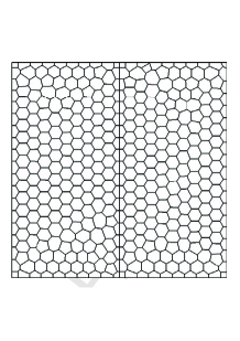
Fig. 2: First mesh of the polygonal mesh sequence.

Numerical experiments are carried out on a sequence of polygonal meshes partitioning the two subdomains $\Omega_{1}$ and $\Omega_{2}$, see Figure 2. To build each polygonal mesh we first generate two matching Delaunay meshes in the left and right parts of $\Omega$ and, then, we build a constraint Voronoi tessellation in each subdomain.

The relative errors for pressure and flux reads as:

$$err(p)=\displaystyle\frac{|||p^{I}-p_{h}|||_{{\cal P}_{h}}}{|||p^{I}|||_{{\cal P}_{h}}};\qquad err(k{\bf u})=\displaystyle\frac{\left(\sum_{c\in\Omega_{h}}|c|\|\widetilde{{\cal K}}_{c}({\bf u}^{I}_{c}-{\bf u}_{c})\|^{2}\right)^{\frac{1}{2}}}{\left(\sum_{c\in\Omega_{h}}|c|\|\widetilde{{\cal K}}_{c}{\bf u}^{I}\|^{2}\right)^{\frac{1}{2}}}.$$

where $p^{I}$ is the interpolation of the exact solution $p$ defined in (3.15), ${\bf u}^{I}$ is the first interpolation of the exact solution gradient ${\bf u}=-\nabla p$ defined in (3.17); $\widetilde{{\cal K}}_{c}$ is the cell-based diagonal matrix formed by coefficients $\widetilde{k}^{c}_{f}$ introduced in Corollary 9. For quasi-uniform meshes considered in the numerical experiments, the Euclidean norm leads to the same conclusions as any reasonable mesh-dependent $L^{2}$ norm.

We report the approximation errors when $k$ is continuous in Table 1 and when $k$ is discontinuous in Table 2. When $k^{c}$ is piecewise constant, the convergence rate of Upwind agrees with the theory since the approximation errors of pressure and flux scale down linearly as expected from estimate (4.69) of Theorem 10 and estimate (4.68) in Corollary 9. In the other cases, a superconvergence effect is visible as the pressure approximation rate is close to $h^{2}$ and the velocity approximation rate is close to $h^{\frac{3}{2}}$. Accordingly, Trace is more accurate than Upwind when $k^{c}$ is piecewise constant, while the accuracy of these schemes is almost the same in the other cases. The superconvergence effect will be investigated in a future work. Finally, the behavior of Trace and Upwind is essentially the same regardless of $k$ being continuous or discontinuous.

Table 1: Relative approximation errors and convergence rates for $p$ and ${\bf u}$ in the case of a continuous diffusion coefficient $k$ using polygonal meshes as the one shown in Figure 2.

	$k^{c}\in{\cal P}^{0}(\Omega_{h})$				$k^{c}\in{\cal P}^{1}(\Omega_{h})$
cells	Trace		Upwind		Trace		Upwind
	err(p)	err(ku)	err(p)	err(ku)	err(p)	err(ku)	err(p)	err(ku)
412	3.220e-3	7.088e-3	7.840e-3	3.877e-2	2.621e-3	3.029e-3	2.629e-3	3.050e-3
1591	7.913e-4	2.251e-3	4.440e-3	1.967e-2	6.442e-3	9.619e-4	6.450e-4	9.656e-4
6433	1.904e-4	8.406e-4	2.627e-3	9.844e-3	1.544e-3	4.407e-4	1.544e-4	4.413e-4
25698	4.716e-5	2.432e-4	1.360e-3	4.818e-3	3.817e-5	1.314e-4	3.819e-5	1.314e-4
102772	1.167e-5	1.123e-4	6.320e-4	2.531e-3	9.513e-6	5.687e-5	9.515e-6	5.688e-5
rate	2.03	1.52	0.90	0.99	2.37	1.44	2.04	1.44

Table 2: Relative approximation errors and convergence rates for $p$ and ${\bf u}$ in the case of a discontinuous diffusion coefficient $k$ using polygonal meshes as the one shown in Figure 2.

	$k^{c}\in{\cal P}^{0}(\Omega_{h})$				$k^{c}\in{\cal P}^{1}(\Omega_{h})$
cells	Trace		Upwind		Trace		Upwind
	err(p)	err(ku)	err(p)	err(ku)	err(p)	err(ku)	err(p)	err(ku)
412	2.762e-3	7.451e-3	5.438e-3	2.679e-2	2.903e-3	3.063e-3	2.588e-3	3.067e-3
1591	6.976e-4	2.370e-3	3.271e-3	1.426e-2	6.540e-4	9.656e-4	6.541e-4	9.637e-4
6433	1.650e-4	9.264e-4	2.242e-3	7.354e-3	1.548e-4	4.897e-4	1.548e-4	4.887e-4
25698	4.066e-5	2.581e-4	1.104e-3	3.690e-3	3.833e-5	1.267e-4	3.832e-5	1.267e-4
102772	1.007e-5	1.134e-4	4.802e-4	2.076e-3	9.502e-6	5.545e-5	9.502e-6	5.543e-5
rate	2.04	1.53	0.86	0.94	2.06	1.45	2.03	1.45

6 Conclusions

Numerical schemes for nonlinear parabolic equations based on harmonic averaging of cell-centered diffusion coefficients at cell interfaces break down when some of these coefficients go to zero or their ratio is too large. To address this issue, in [38] we proposed a new family of second-order accurate mimetic finite difference schemes on polygonal and polyhedral meshes. In this new discrete setting the primary mimetic operator approximates the continuum operator $\textsf{div}(k\,\cdot\,)$, while the derived (dual) mimetic operator approximates $\nabla(\cdot)$. The discrete divergence operator requires a staggered discretization of the diffusion coefficient, one value per mesh cell and up to two values per mesh face. The availability of face diffusion coefficients provides more flexibility in the numerical formulation, which can be exploited to design robust numerical algorithms for nonlinear problems. For instance, upwinding of the diffusion coefficients on mesh faces can be easily incorporated into the new mimetic schemes. The new mimetic method applied to the steady diffusion equation in mixed form is proved to be well-posed since it satisfies the discrete inf-sup condition, and convergent by deriving first-order error estimates for the scalar and gradient unknowns. Numerical experiments verify the theory.

References

• [1] R. A. Adams and J. J. F. Fournier. Sobolev spaces, volume 140 of Pure and Applied Mathematics (Amsterdam). Elsevier/Academic Press, Amsterdam, second edition, 2003.
• [2] T. Arbogast, C.N. Dawson, P.T. Keenan, M.F. Wheeler, and I. Yotov. Enhanced cell-centered finite differences for elliptic equations on general geometry. SIAM J. Sci. Comput., 19(2):404–425, 1998.
• [3] T. Arbogast, M. F. Wheeler, and I. Yotov. Mixed finite elements for elliptic problems with tensor coefficients as cell-centered finite differences. SIAM Journal on Numerical Analysis, 34(2):828–852, 1997.
• [4] L. Beirão da Veiga, J. Droniou, and G. Manzini. A unified approach to handle convection terms in Finite Volumes and Mimetic Discretization Methods for elliptic problems. IMA J. Numer. Anal., 31(4):1537–1541, 2011.
• [5] L. Beirão da Veiga, V. Gyrya, K. Lipnikov, and G. Manzini. Mimetic finite difference method for the Stokes problem on polygonal meshes. J. Comput. Phys., 228(19):7215–7232, 2009.
• [6] L. Beirão da Veiga, K. Lipnikov, and G. Manzini. Convergence analysis of the high-order mimetic finite difference method. Numer. Math., 113(3):325–356, 2009.
• [7] L. Beirão da Veiga, K. Lipnikov, and G. Manzini. Error analysis for a mimetic discretization of the steady Stokes problem on polyhedral meshes. SIAM Journal on Numerical Analysis, 48(4):1419–1443, 2010.
• [8] L. Beirão da Veiga, K. Lipnikov, and G. Manzini. Arbitrary order nodal mimetic discretizations of elliptic problems on polygonal meshes. SIAM Journal on Numerical Analysis, 49(5):1737–1760, 2011.
• [9] L. Beirão da Veiga and G. Manzini. An a posteriori error estimator for the mimetic finite difference approximation of elliptic problems. Int. J. Numer. Meth. Engrg., 76(11):1696–1723, 2008.
• [10] L. Beirão da Veiga and G. Manzini. A higher-order formulation of the mimetic finite difference method. SIAM Journal on Scientific Computing, 31(1):732–760, 2008.
• [11] L. Beirao da Veiga, F. Brezzi, L. D. Marini, and A. Russo. Mixed virtual element methods for general second order elliptic problems on polygonal meshes. ESAIM: Mathematical Modelling and Numerical Analysis, 50(3):727–747, 2016.
• [12] L. Beirao da Veiga and A. Ern. Preface. ESAIM: M2AN, 50(3):633–634, 2016. Special Issue - Polyhedral discretization for PDEs.
• [13] L. Beirao da Veiga, K. Lipnikov, and G. Manzini. The Mimetic Finite Difference Method for Elliptic PDEs. Springer, 2014. 408 pages.
• [14] N. Bellomo, F. Brezzi, and G. Manzini. Recent techniques for pde discretizations on polyhedral meshes. Math. Models Methods Appl. Sci., 24:1453–1455, 2014. (special issue).
• [15] D. Boffi, F. Brezzi, and M. Fortin. Mixed Finite Element Methods and Applications. Springer Series in Computational Mathematics. Springer, Berlin, Heidelberg, 2013.
• [16] S. C. Brenner and L. R. Scott. The mathematical theory of finite element methods. Texts in applied mathematics. Springer, New York, Berlin, Paris, 2002.
• [17] F. Brezzi, A. Buffa, and K. Lipnikov. Mimetic finite differences for elliptic problems. M2AN Math. Model. Numer. Anal., 43(2):277–295, 2009.
• [18] F. Brezzi, R. S Falk, and L. D. Marini. Basic principles of mixed virtual element methods. ESAIM: Mathematical Modelling and Numerical Analysis, 2014.
• [19] F. Brezzi, K. Lipnikov, and M. Shashkov. Convergence of the mimetic finite difference method for diffusion problems on polyhedral meshes. SIAM J. Numer. Anal., 43(5):1872–1896, 2005.
• [20] F. Brezzi, K. Lipnikov, and M. Shashkov. Convergence of mimetic finite difference method for diffusion problems on polyhedral meshes with curved faces. Math. Models Methods Appl. Sci., 16(2):275–297, 2006.
• [21] F. Brezzi, K. Lipnikov, and V. Simoncini. A family of mimetic finite difference methods on polygonal and polyhedral meshes. Math. Models Methods Appl. Sci., 15(10):1533–1551, 2005.
• [22] A. Cangiani, F. Gardini, and G. Manzini. Convergence of the mimetic finite difference method for eigenvalue problems in mixed form. Comput. Methods Appl. Mech. Engrg., 200(9–12):1150–1160, 2011.
• [23] A. Cangiani and G. Manzini. Flux reconstruction and pressure post-processing in mimetic finite difference methods. Comput. Methods Appl. Mech. Engrg., 197/9-12:933–945, 2008.
• [24] A. Cangiani, G. Manzini, and A. Russo. Convergence analysis of the mimetic finite difference method for elliptic problems. SIAM J. Numer. Anal., 47(4):2612–2637, 2009.
• [25] J.I. Castor. Radiation Hydrodynamics. Cambridge University Press, 2004.
• [26] B. Cockburn, D. A. Di Pietro, and A. Ern. Bridging the hybrid high-order and hybridizable discontinuous Galerkin methods. ESAIM: Mathematical Modelling and Numerical Analysis, 50(3):635–650, 2016.
• [27] D. A. Di Pietro and A. Ern. Hybrid high-order methods for variable-diffusion problems on general meshes. Comptes Rendus Mathématique, 353(1):31–34, 2015.
• [28] J. Droniou and R. Eymard. A mixed finite volume scheme for anisotropic diffusion problems on any grid. Numer. Math., 105(1):35–71, 2006.
• [29] J. Droniou, R. Eymard, and R. Herbin. Gradient schemes: Generic tools for the numerical analysis of diffusion equations. ESAIM: Mathematical Modelling and Numerical Analysis, 50(3):749–781, 2016.
• [30] J. Droniou, N. Nataraj, and S. Devika. Gradient schemes for optimal control problems, with super-convergence for non-conforming finite elements and mixed-hybrid mimetic finite differences. arXiv preprint arXiv:1608.01726, 2016.
• [31] R. Eymard, T. Gallouët, and R. Herbin. The finite volume method. In P. Ciarlet and J.L. Lions, editors, Handbook for Numerical Analysis, pages 715–1022. North Holland, 2000.
• [32] R. Eymard, T. Gallouet, and R Herbin. Finite volume approximation of elliptic problems and convergence of an approximate gradient. Applied Numerical Mathematics, 37(1):31–53, 2001.
• [33] R. Eymard, T. Gallouet, and R. Herbin. Discretization of heterogeneous and anisotropic diffusion problems on general non-conforming meshes. SUSHI: a scheme using stabilization and hybrid interface, 2009. IMA J. Numer. Anal.
• [34] R. Eymard, G. Henri, R. Herbin, R. Klofkorn, and G. Manzini. 3D Benchmark on discretizations schemes for anisotropic diffusion problems on general grids. In J. Fort, J. Furst, J. Halama, R. Herbin, and F. Hubert, editors, Finite Volumes for Complex Applications VI. Problems & Perspectives, volume 2, pages 95–130, Prague, June 6–11 2011. Springer.
• [35] V. Gyrya, K. Lipnikov, G. Manzini, and D. Svyatskiy. M-adaptation in the mimetic finite difference method. Math. Models Methods Appl. Sci., 24:1621–1663, 2014.
• [36] J. M. Hyman and M. Shashkov. Approximation of boundary conditions for mimetic finite-difference methods. Computers & Mathematics with Applications, 36(5):79 – 99, 1998.
• [37] K. Lipnikov, G. Manzini, F. Brezzi, and A. Buffa. The mimetic finite difference method for 3D magnetostatics fields problems. Journal of Computational Physics, 230(2):305–328, 2011.
• [38] K. Lipnikov, G. Manzini, J. D. Moulton, and M. Shashkov. The mimetic finite difference method for elliptic and parabolic problems with a staggered discretization of diffusion coefficient. J. Comput. Phys, 305:111–126, 2016. http://dx.doi.org/10.1016/j.jcp.2015.10.031.
• [39] K. Lipnikov, G. Manzini, and M. Shashkov. Mimetic finite difference method. J. Comp. Phys., 257:1163–1227, 2014.
• [40] K. Lipnikov, G. Manzini, and D. Svyatskiy. Analysis of the monotonicity conditions in the mimetic finite difference method for elliptic problems. J. Comput. Phys., 230(7):2620 – 2642, 2011.
• [41] K. Lipnikov, J. Morel, and M. Shashkov. Mimetic finite difference methods for diffusion equations on non-orthogonal non-conformal meshes. J. Comput. Phys., 199, 2004.
• [42] G. Manzini, A. Russo, and N. Sukumar. New perspectives on polygonal and polyhedral finite element methods. Mathematical Models & Methods in Applied Sciences, 24(8):1621–1663, 2014.
• [43] L.A. Richards. Capillary conduction of liquids through porous mediums. Physics 1, 5:318–333, 1931.
• [44] M. Shashkov and S. Steinberg. Solving diffusion equations with rough coefficients in rough grids. Journal of Computational Physics, 129(2):383 – 405, 1996.
• [45] J. Wang and X. Ye. A weak Galerkin mixed finite element method for second-order elliptic problems, 2013. arXiv:1202.3655v3.