Instabilities and spin-up behaviour of a rotating magnetic field driven flow in a rectangular cavity

Abstract

This study presents numerical simulations and experiments considering the flow of an electrically conducting fluid inside a cube driven by a rotating magnetic field (RMF). The investigations are focused on the spin-up, where a liquid metal (GaInSn) is suddenly exposed to an azimuthal body force generated by the RMF, and the subsequent flow development. The numerical simulations rely on a semi-analytical expression for the induced electromagnetic force density in an electrically conducting medium inside a cuboid container with insulating walls. Velocity distributions in two perpendicular planes are measured using a novel dual-plane, two-component ultrasound array Doppler velocimeter (UADV) with continuous data streaming, enabling long term measurements for investigating transient flows. This approach allows to identify the main emerging flow modes during the transition from a stable to unstable flow regimes with exponentially growing velocity oscillations using the Proper Orthogonal Decomposition (POD) method.

Characteristic frequencies in the oscillating flow regimes are determined in the super critical range above the critical magnetic Taylor number $Ta_{c}\approx 1.26\times 10^{5}$, where the transition from the steady double vortex structure of the secondary flow to an unstable regime with exponentially growing oscillations is detected.

The mean flow structures and the temporal evolution of the flow predicted by the numerical simulations and observed in experiments are in very good agreement.

I Introduction

Electromagnetic flow control is an important and efficient tool for optimizing fluid flow and transport processes in crystal growth, metallurgy and metal casting. Various types of tailored AC magnetic fields are applied for electromagnetic stirring providing a variable and contact-less access to electrically conducting melts (see Gerbeth et al. Gerbeth, Eckert, and Odenbach (2013) and references therein). The specific requirements arising from the particular metallurgical or casting operation are manifold. For instance, the electromagnetic stirring should provide an efficient mixing of the melt or counterbalance buoyancy-driven flows. Different types of magnetic fields (as rotating, travelling, pulsating and combinations of these three) are available, whereas each field type gives rise to a more or less distinctive flow pattern. A deep understanding of the fluid flow properties under the effect of AC magnetic fields is required for defining optimal configurations and parameters for the magnetic system. Within this study we consider the case of rotary stirring in a square cross-section, for which the process of billet or bloom casting in steel production can serve as a prominent example from industrial practice. Fabricating multicrystalline silicon for photovoltaic modules often involves a rectangular crucible cross section and time-varying magnetic fields from resistive heaters. A great deal of work has been done yet for investigating the properties of fluid flow driven by a rotating magnetic field (RMF) inside a cylindrical vessel. For a detailed review about RMF-driven flows we refer the reader to the classical paper of Davidson and Hunt Davidson and Hunt (1987) or Priede and Gelfgat Gelfgat, Grants, and Priede (1995). The transition from a steady to a time-dependent flow regime was studied among others by Barz et al. Barz et al. (1997), Kaiser and Benz Kaiser and Benz (1998) and Witkowski et al. Witkowski, Walker, and Marty (1999). The authors tried to find a critical non-dimensional magnetic Taylor number for the onset of the instabilities using different methods for direct numerical simulation. Recently, Grants and Gerbeth Grants and Gerbeth (2001, 2002, 2003) conclude that the RMF-driven flows in a cylinder become unstable first to non-axisymmetric, azimuthally periodic perturbations at diameter-to-height aspect ratios $AR$ between $0.5$ and $2$. Ungarish Ungarish (1997) and Nikrityuk et al. Nikrityuk et al. (2005) considered the so-called spin-up process of a developing flow when the fluid at rest is exposed to a suddenly applied RMF. The numerical simulations were confirmed experimentally by flow measurements performed by Räbiger et al. Räbiger, Eckert, and Gerbeth (2010). Evolving perturbations of the double vortex structure just above the instability threshold occur in form of Taylor–Görtler vortices. The rotational symmetry of the flow structure is kept while a first Taylor–Görtler vortex pair has been formed as closed rings along the cylinder perimeter. The transition to a three-dimensional flow in the side layers occurs by advection, precession and splitting of the Taylor - Görtler vortex rings Vogt et al. (2012).

In contrast, the number of studies dealing with rotary stirring in square or rectangular cross sections appears to be rather small. Dubke et al. Dubke et al. (1988a, b) presented a theoretical model for describing the electromagnetic forces and fluid flow occurring in electromagnetic stirring of continuously cast strands with a rectangular cross-section. Experiments were carried out in a cold model for verifying the calculations. However, the flow velocity measurements performed rely on photographical techniques or a drag probe, respectively. Both approaches do not allow for quantitative flow measurements at high spatial and temporal resolution.

A numerical study of an RMF-driven flow in a square container was published by Frana and Stiller Frana and Stiller (2008). The authors found that the velocity field is influenced by the corner effects and exhibits a non-axisymmetric structure in a wide range of magnetic Taylor numbers. In this study the investigations are focused on the spin-up process resulting from the application of the electromagnetic driving force in form of a step function to the fluid being at rest in the initial state. The magnetic field was initiated at the time $t=0$ and induces a mainly azimuthal body force inside the liquid driving a primary swirling flow. The centrifugal force changes across the boundary layers at the horizontal walls of the container. This is balanced by a radial pressure gradient resulting in a liquid flow towards the cylinder axis inside the horizontal boundary layers. This mechanism also known as Ekman pumping is responsible for the existence of the secondary flow appearing as double vortex in the radial-vertical plane.

In this paper we present a combined experimental and numerical study devoted to the transitional behaviour of the flow in a cubic container driven by a rotating magnetic field. The paper is organized as follows: the experimental setup and its instrumentation is presented in section II. The governing equation for describing the induced electromagnetic field in the liquid melt and specially the derivation of a semi-analytical expression for the time average of the induced electromagnetic force density in the electrically conducting medium are described in detail in section III. In section IV we present and discuss the main results of the numerical simulation and the measurements in the experiments. In order to obtain a better understanding of the transitions between different flow regimes we perform a Proper Orthogonal Decomposition (POD) of both, the numerical simulation and the measurements. This study leads to the identification of the characteristic exponential growth of the first emerging flow instabilities. The characteristic frequencies and growth rates are estimated. The results are summarized in section V.

II Experimental setup

The experiments are conducted using the eutectic alloy GaInSn, enclosed in a cubic container made of acrylic glass with an edge length of $2L={67.5}\,\mathrm{mm}$. Due to the low melting point, $\vartheta_{m}={10}\,\mathrm{{}^{\circ}C}$, the metal is liquid at room temperature. The container is positioned in the center of the magnetic system MULTIMAG (MULTI purpose MAGnetic field) facility, which is capable of generating different types of magnetic fields of varying strength and frequency with high accuracy Pal et al. (2009). The magnetic system consists of a radial arrangement of six coils, whereby opposing coils are connected as pole-pairs. A three-phase current generates a horizontal RMF rotating in the horizontal plane in clockwise direction with a frequency of ${50}\,\mathrm{Hz}$. The symmetry axes of magnetic field and fluid container are identical. The origin of the coordinates is collocated in the center of the cube. Special care was taken to ensure a precise positioning of the cube inside the magnetic field for avoiding flow artifacts caused by a misplacement of the fluid volume with respect to the magnetic field. The homogeneity of the magnetic field was checked using a 3-axis Gauss meter (Lakeshore model 560, sensor type MMZ2560-UH) and was found to be better than 3 %.

The fluid velocity was measured using the ultrasound Doppler velocimetry (UDV), which allows for determining instantaneous velocity profiles in opaque fluids Takeda (1991). The measuring principle is based on the pulse - echo technique and uses short ultrasound bursts emitted from an ultrasound transducer, that reflecte from acoustic inhomogeneities moving inside the fluid and are received from the transducer. In case of GaInSn, these inhomogeneities are assumed to be microscopic oxide particles The measurements rely on the assumption, that the reflecting particles are homogeneously dispersed in the melt and follow the flow without slip. Velocity profiles are reconstructed using information about (i) the distance between the UDV-transducer and the reflecting particle which is derived from the time of flight of the ultrasound burst and (ii) the velocity component along the beam direction which is determined from the phase shift of subsequent ultrasound burst echos.

Within this study we applied an ultrasound array Doppler velocimeter (UADV)  Franke et al. (2010); Nauber et al. (2013) in order to perform a two-dimensional flow mapping in both the horizontal and vertical mid-plane of the cube. In our study the cube is instrumented with four linear ultrasound arrays arranged orthogonally. Such an arrangement provides a two-dimensional mapping of the two in-plane velocity components (cf. Fig. 1).

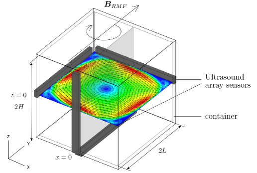
Figure 1: Measurement configuration: a cubical vessel filled with GaInSn, instrumented with four ultrasound array sensors. An example for a typical reconstructed vortex flow in the horizontal plane is shown here. The color represents the intensity of the flow and the arrows the direction in the plane.

Each array consists of $25$ transducers with the dimensions of ${2.5\times 5}\,\mathrm{mm^{2}}$ resulting in a total sensitive length of ${67.5}\,\mathrm{mm}$ (cf. Fig. 2). A pairwise excitation of neighboring elements gives an active surface of ${5\times 5}\,\mathrm{mm^{2}}$ associated with a sound beam width of approximately ${3}\,\mathrm{mm}$ in GaInSn. The excitation signal is eight periods of a sine wave at $f={8}\,\mathrm{MHz}$ resulting in an axial resolution of about ${1.4}\,\mathrm{mm}$ Franke et al. (2013). The acoustical impedance of the transducers is matched to PMMA (${3.4}\,\mathrm{MRayl}$), which maximizes the sound transmission through the sensor - wall interface.

Figure 2: Geometrical dimensions of the ultrasound array sensor, the marked elements are active during the first scanning step.

In order to acquire a planar velocity map, an electronic scanning of the respective linear sensor arrays is performed. The frame-rate is increased over a simple sequential scan by parallelizing the measurement based on a combined space division/time division multiplexing scheme Franke et al. (2013). In this way a frame-rate of up to ${33}\,\mathrm{Hz}$ can be achieved in the given configuration. To avoid crosstalk between the sensor arrays in this configuration, all four arrays are driven sequentially.

The velocity information is extracted from the amplified and digitized ultrasound (US) echo signals via the Kasai autocorrelation method Kasai et al. (1985). A typical mean data bandwidth after digitalization is ${1.2}\,\mathrm{GB/s}$, which is beyond the limit that can be acquired and stored continuously with common PC hardware. Therefore a real-time data compression is performed by offloading parts of the signal processing to a field-programmable gate array (FPGA, NI PXIe-7965R). The preprocessing reduces the amount of data by 10:1 and enables a continuous streaming for a practically unlimited duration Nauber et al. (2016).

III Governing equations

Let us consider the flow of an electrically conducting fluid with kinematic viscosity $\nu$, density $\rho$ and electrical conductivity $\sigma$ in a cuboid container with the basis edge length $2L$ and the height $2H$ driven by a uniform magnetic field of induction $B_{0}$ rotating around the vertical axis $\boldsymbol{e}_{z}$ with a constant angular frequency $\omega$.

III.1 Induced electromagnetic force

In the scope of the low-induction approximation (very small magnetic Reynolds number $R_{m}=\mu_{0}\sigma u_{0}L<<1$) the electro-motive field $\boldsymbol{u}\times\boldsymbol{B}$ can be neglected compared to the induced electric field $\boldsymbol{E}$ within the Ohm’s law $\boldsymbol{j}=\sigma(\boldsymbol{E}+\boldsymbol{u}\times\boldsymbol{B})$. Here is $\mu_{0}$ the magnetic vacuum permeability and $u_{0}$ is a characteristic velocity of the flow. The back reaction of the flow field $\boldsymbol{u}$ on the total induced electric current density $\boldsymbol{j}$ can be neglected, too. This is why the simulations of the electromagnetic field and the fluid flow can be conducted separately. Hence, a quasi - analytical expression for the time-averaged electromagnetic force density $\boldsymbol{j}\times\boldsymbol{B}$ acting on the liquid metal in the cavity can be derived.

A clockwise rotating magnetic field with strength $B_{0}$ can be expressed as:

$$\boldsymbol{B}=B_{0}\left\{cos(\omega t)\boldsymbol{e}_{x}-sin(\omega t)\boldsymbol{e}_{y}\right\}\,.$$ (1)

The corresponding magnetic vector potential ($\boldsymbol{B}=\nabla\times\boldsymbol{A}$) has only one axial component: $\boldsymbol{A}=B_{0}\left(y\,cos(\omega t)+x\,sin(\omega t)\right)~{}\boldsymbol{e}_{z}$. The unit vectors $\boldsymbol{e}_{x}$, $\boldsymbol{e}_{y}$ and $\boldsymbol{e}_{z}$ are related to the axes of the reference system and their orientation is sketched in Fig. 1.

Within the considered approximation the electric current density can be calculated using the Ohm’s law and the first Maxwell’s equation:

$$\boldsymbol{j}=\sigma\boldsymbol{E}=\sigma\{-\nabla\Phi-\frac{\partial\boldsymbol{A}}{\partial t}\}=\sigma\left\{-\nabla\Phi-B_{0}\omega\left(-y\,sin(\omega t)+x\,cos(\omega t)\right)\boldsymbol{e}_{z}\right\}\,.$$ (2)

Here is $\Phi$ the electric potential. The induced currents have been neglected in the frame of the low frequency approximation assuming a complete penetration of the fluid volume by the magnetic field. In a next step we compute the instantaneous electromagnetic force density taking into account the expressions 1 and 2:

$$\boldsymbol{j}\times\boldsymbol{B} = \sigma B_{0}\{(-\frac{\partial\Phi}{\partial z}-\omega B_{0}(-ysin(\omega t)+xcos(\omega t)))(sin(\omega t)~{}\boldsymbol{e}_{x}+cos(\omega t)~{}\boldsymbol{e}_{y})$$ (3)

$$+(\frac{\partial\Phi}{\partial y}cos(\omega t)+\frac{\partial\Phi}{\partial x}sin(\omega t))\boldsymbol{e}_{z}\}\,.$$

Until this point the equation 3 shows the same form as presented in the paper from Frana and Stiller Frana and Stiller (2008). Now we obtain a semi-analytical expression for the electromagnetic force density using a proper ansatz for the electric potential $\Phi$:

$$\Phi(x,y,z,t)=\omega B_{0}(a(x,y,z)cos(\omega t)+b(x,y,z)sin(\omega t))\,.$$ (4)

The functions $a(x,y,z)$ and $b(x,y,z)$ have the dimensions $\mathrm{m}^{2}$. Whilst taking into account that $1/T\int_{0}^{T}dt~{}sin^{2}(\omega t)=1/T\int_{0}^{T}dt~{}cos^{2}(\omega t)=1/2$ we perform now the time averaging of the force density defined in Eq. 3 over a period $T=2\pi/\omega$ in order to separate its steady part:

$$\boldsymbol{f}=<\boldsymbol{j}\times\boldsymbol{B}>_{T}=\frac{\sigma\omega B_{0}^{2}}{2}\left\{(-\frac{\partial b}{\partial z}+y)~{}\boldsymbol{e}_{x}+(-\frac{\partial a}{\partial z}-x)~{}\boldsymbol{e}_{y}+(\frac{\partial b}{\partial x}+\frac{\partial a}{\partial y})~{}\boldsymbol{e}_{z}\right\}\,.$$ (5)

The Kirchhoff’s law for the electric charge conservation $\nabla\cdot\boldsymbol{j}=0$ leads to the equation for the electric potential $\nabla^{2}\Phi=0$. Using the ansatz 4, we obtain the following system of equations:

$$\nabla^{2}a=0\quad\mbox{and}\quad\nabla^{2}b=0$$ (6)

which should be solved under the boundary condition excluding any electrical current flowing through isolating walls ($j_{n}=0$). It means, for example, for the functions $a$:

$$\frac{\partial a}{\partial z}|_{z=\pm H}=-x\quad\mbox{and}\quad\frac{\partial a}{\partial x}|_{x=\pm L}=\frac{\partial a}{\partial y}|_{y=\pm L}=0\,.$$ (7)

Due to reasons of symmetry, it can be shown that $a(x,y,z)=a(x,z)=-b(y,z)$. This fact leads to the following final expression for the time averaged electromagnetic force density:

$$\boldsymbol{f}=\frac{\sigma\omega B_{0}^{2}}{2}\left\{(\frac{\partial a}{\partial z}(y,x,z)+y)~{}\boldsymbol{e}_{x}+(-\frac{\partial a}{\partial z}(x,y,z)-x)~{}\boldsymbol{e}_{y}\right\}\,.$$ (8)

The functions $a$ and $b$ are solutions of the equation 6 on the boundary conditions 7. Using $L$ as length scale and $\rho\nu^{2}/L^{3}$ as the scale for the force volume density we can express equation 8 in a dimensionless form $\boldsymbol{f}=Ta~{}\boldsymbol{f}_{EM}$ with

$$\boldsymbol{f}_{EM}=r~{}\boldsymbol{e}_{\varphi}+\left(-\frac{\partial b}{\partial z}~{}\boldsymbol{e}_{x}-\frac{\partial a}{\partial z}~{}\boldsymbol{e}_{y}\right)\quad\mbox{and}\quad Ta=\frac{\displaystyle\sigma\omega B_{0}^{2}L^{4}}{\displaystyle 2\rho\nu^{2}}\,.$$ (9)

$Ta$ denotes the magnetic Taylor number, which is an expression for the relative strength of the electromagnetic force driving the flow.

The first term in equation 9 is strictly azimuthal and linear in the polar radius $r=\sqrt{x^{2}+y^{2}}$ and the second term takes into consideration the geometry of the cross section and the finite height of the container.

Fig. 3 shows the spatial distribution of the time-averaged non-dimensional electromagnetic force density $\boldsymbol{f}_{EM}$, which was added as an additional body force to the Navier Stokes equation for the case of an aspect ratio $H/L=1$. The force reaches its maximum value $\boldsymbol{f}_{{EM}_{max}}=0.953$ at half height in a vertical edge of the cube, i.e. for example at the position with the coordinates $x=1,y=1,z=0$.

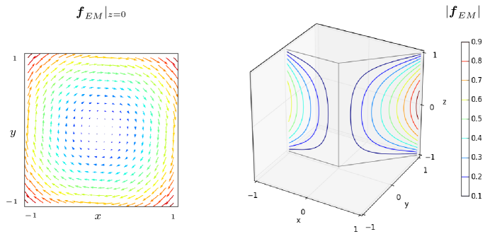
Figure 3: Simulation: Vector plot (left) and amplitude (right) of the non-dimensional electromagnetic force density $\boldsymbol{f}_{EM}$ (Eq. 9) at different sectional planes.

The electromagnetic force density distribution for arbitrary aspect ratios can be determined by the procedure described herein. A study of the RMF induced flow for different aspect ratios will be published in the future, however, this paper focuses on the aspect ratio $H/L=1$, which is realized in the experimental setup.

III.2 Electromagnetically driven flow

The numerical simulations of the liquid metal flow are performed using the open source code library OpenFOAM^© 3.0.x OpenCFD (2015). The flow was computed solving the incompressibility condition $\nabla\cdot\boldsymbol{u}=0$ and the incompressible Navier-Stokes equation in a dimensionless form, with $L$, $L^{2}/\nu$ and $\rho(\nu/L)^{2}$ being the distance, time and pressure scale, respectively, is given by

$$\frac{\partial\boldsymbol{u}}{\partial t}+(\boldsymbol{u}\cdot\nabla)\boldsymbol{u}=-\nabla p+\nabla^{2}\boldsymbol{u}+Ta~{}\boldsymbol{f}_{EM}\,.$$ (10)

The no-slip condition $u=0$ at the solid container walls was chosen as boundary condition for the calculation of the flow field.

The set of equations is solved using the PISO (Pressure Implicit with Splitting Operator) algorithm Issa (1986); Ferziger and Peric (2003) on a collocated grid. The time step was chosen so that the Courant number always remains below 0.25. We use a structured numerical grid with two million volume elements and refinements near the walls. Second order accurate schemes are used for time (Crank-Nicolson) and space discretization (linear scheme).

In order to obtain mesh refinement independent solutions reliably, we performed mesh convergence studies using 4 different discrete meshes with $10^{6}$ (mesh I), $1.57\times 10^{6}$ (mesh II), $2\times 10^{6}$ (mesh III) and $2.46\times 10^{6}$ (mesh IV) number of cells, respectively. For the mesh generation we used the standard blockMesh OpenFOAM tool with multi-grading. We stretched the mesh between $x=0.9$ and $x=1$ (wall) with a stretching factor of $\Delta x_{max}/\Delta x_{min}=5$. Doing so, the maximum volume aspect ratio remain less than 0.5. The smallest cell edge length is $\Delta x_{min}=0.00329$ and the boundary layer region between $x=0.9$ and $x=1$ contains 12 cells. In Sec. IV.2, we show the results of the convergence studies at different typical flow regimes.

IV Results and discussion

In this section we present numerical and experimental results with respect to the flow of GaInSn driven by a rotating magnetic field with strength $B_{0}$ in a closed cube with edge length $2L={67.5}\,\mathrm{mm}$ For the numerical simulations the following material properties of Ga₆₇In_20.5Sn_12.5 in wt. % at ${20}\,\mathrm{{}^{\circ}C}$ were usedPlevachuk et al. (2014):

density	$~{}\rho$ :	$6403$	${}\,\mathrm{kg/m^{3}}$
viscosity	$~{}\nu$ :	$0.34\times 10^{-6}$	${}\,\mathrm{m^{2}/s}$
conductivity	$~{}\sigma$ :	$3.29\times 10^{6}$	${}\,\mathrm{S/m}$

This results in a viscous time scale of $t_{0}=L^{2}/\nu={3341.23}\,\mathrm{s}$ and a velocity scale $u_{0}=\nu/L={0.0101}\,\mathrm{mm\,s^{-1}}$. Everything that is presented in this paper from now on will be given in a dimensionless form taking into account the previously introduced scaling.

IV.1 Steady flow regime

Below the critical value of the magnetic Taylor number $Ta_{c}$ the electromagnetically driven flow remains laminar and steady. In Sec. IV.2, we will identify this critical value by analyzing both the time-dependent numerical simulations and the flow measurements carried out during the experiments. In both cases, the flow becomes unsteady beyond $Ta>1.3\times 10^{5}$.

For a better understanding and a better description of the development of the main flow structures we split the velocity field $\boldsymbol{u}$ in two parts: the so-called primary flow, which contains the azimuthal component only $u_{\varphi}\boldsymbol{e}_{\varphi}$ and the remaining part $\boldsymbol{u}-u_{\varphi}\boldsymbol{e}_{\varphi}$, which we call secondary flow.

In general, the flow structure changes rapidly for increasing driving force strength. For very small values of the Taylor number, i.e. $Ta<10$, the flow structure shows mirror symmetries with respect to the $x$,$y$ and $z$ planes (cf. Fig. 4).

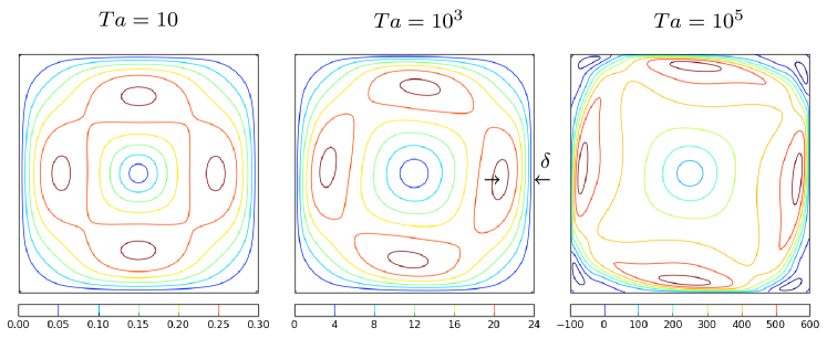
Figure 4: Simulation: Contours of the azimuthal flow velocity $-u_{\varphi}$ at the middle horizontal plane $z=0$ show the decreasing of the boundary layer size $\delta$ and the loss of the mirror symmetry with respect to the $x$ and $y$ planes for increasing values of the Taylor number $Ta$.

The increase of the Taylor number causes a remarkable deformation of the contour lines of the azimuthal flow velocity $u_{\varphi}=−u_{x}sin(\varphi)+u_{y}cos(\varphi)$. The higher the chosen $Ta$, the narrower the boundary layers of the azimuthal velocity are formed in the vicinity of the container walls. This represents a challenge for both the numerical simulation and the measurements with respect to ensuring an appropriate resolution near the wall. Within this study the use of stretched meshes in the numerical simulations guarantees a sufficient resolution of the boundary layers. Starting from the center axis the azimuthal velocity increases linearly with the distance from the vertical axis. It achieves a maximum value at certain position $\boldsymbol{r}_{m}$ and finally it decreases to zero value at the side wall. The thickness of the boundary layer for the azimuthal velocity can be defined as the distance between the place where the azimuthal velocity has a maximum and the side wall, i.e. $\delta=1-\boldsymbol{r}_{m}\cdot\boldsymbol{e}_{x}$.

Fig. 4 reveals that for high values of the magnetic Taylor number $Ta$ (i.e. for $Ta>6\times 10^{3}$) small regions in the vicinity of the corners appear where the fluid rotates in a direction opposite to the main rotation direction. This causes the shear to increase and thus the tendency for the formation of flow instabilities.

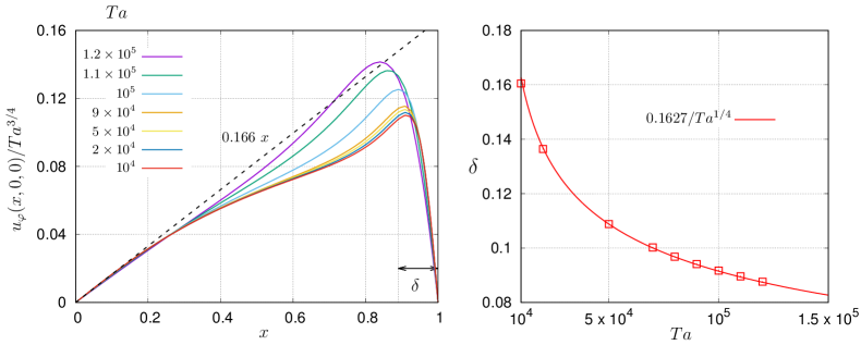
Figure 5: Simulation: Azimuthal velocity profiles at the middle horizontal plane (left) and boundary layer thickness $\delta$ (right) for different values of the Taylor number

Fig. 5 shows the azimuthal velocity profiles at the middle horizontal plane ($u_{\varphi}(x,0,0)$, left) and the boundary layer thickness $\delta$ (right) for different values of the Taylor number. The latter scales like $\delta=1.627~{}Ta^{-1/4}$. Applying the scale $Ta^{3/4}$ for the azimuthal velocity, the core rotation speed $\Omega=u_{\varphi}/r|_{r\to 0}$ shows a self similar behaviour, i.e. $\Omega=0.166~{}Ta^{3/4}$ is obtained for $0.2\times 10^{4}<Ta<1.5\times 10^{5}$ in a contrast to different scaling behaviours discussed in Nikrityuk et al. (2005) for the case of the RMF flow in a cylindrical container ($\Omega\propto Ta^{2/3}$ in that case). This means for example in physical units, that for $Ta=10^{5}$ the central core rotates with an almost constant angular velocity $\Omega={0.278}\,\mathrm{s^{-1}}$ while the RMF does this with the angular frequency $\omega=2\pi\times{50}\,\mathrm{s^{-1}}$. The boundary layer thickness for $Ta=10^{5}$ is $\delta=0.0917$. Within this region the grid is stretched, it contains 11 cells and the smallest cell edge length is 0.00358 in non-dimensional units. This fact guarantees a correct description of the boundary layer.

Let us examine the scaling behaviour of the maximum velocity of the primary flow at the central horizontal plane $z=0$ with respect to the magnetic Taylor number $Ta$. For an infinitely long circular cylinder an analytical expression for the velocity field exists under the assumptions that the flow is laminar and that the velocity field has only one azimuthal component depending on the polar radius only: $u_{\varphi}(r)=r~{}(1-r^{2})~{}Ta/8$. The maximum velocity value ${u_{\varphi}}_{max}=Ta/(12\sqrt{3})$ is directly proportional to the Taylor number $Ta$. In the case of the RMF-driven flow in a cubic container as studied here, the azimuthal velocity profile along a horizontal line exhibits a similar behaviour. Figure 6 shows the $Ta$ number dependence of the maximum Reynolds number associated with the primary flow

$$Re_{max}=max\{\sqrt{(u_{x}^{2}+u_{y}^{2})}|_{z=0}\}$$ (11)

from the numerical simulation and the measurements.

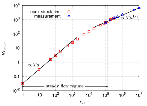
Figure 6: Scaling behaviour: Maximum Reynolds number of the primary flow $Re_{max}$ (cf. Eq. 11) as a function of the magnetic Taylor number $Ta$.

Figure 6 reveals two characteristic asymptotic scaling laws. A linear relationship appears for small values of the Taylor number ($Ta<2\times 10^{2}$): $Re_{max}\approx 0.031~{}Ta$. The corresponding relation for the laminar flow in an infinitely long circular cylinder is rather similar, namely $Re_{max}=Ta/(12\sqrt{3})$. For $Ta>4\times 10^{5}$ we find the relationship $Re_{max}\approx 2.08~{}Ta^{1/2}$ in concordance with the predictions made by Davidson and Hunt Davidson and Hunt (1987).

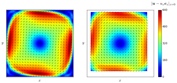
Figure 7: Velocity distribution of the primary flow ($u_{x}\boldsymbol{e}_{x}+u_{y}\boldsymbol{e}_{y})|_{z=0}$ for $Ta=10^{5}$ (left: computed steady state from the numerical simulation, right: measured mean values)

Fig. 7 shows velocity distributions of the primary flow in the horizontal plane $z=0$ (i. e., $(u_{x}\boldsymbol{e}_{x}+u_{y}\boldsymbol{e}_{y})|_{z=0}$) computed from the numerical simulation (left) and measured during the experiments (right) for $Ta=10^{5}$. The measured values presented here were averaged over the time interval $1000-{2000}\,\mathrm{s}$. This direct comparison reveals a very good agreement. The flow pattern reconstructed from the UADV measurements by interpolation does not fill the entire cross section. Due to the dimensions of the sensor housing and constructive limitations of the container design the flow field cannot be acquired in the immediate vicinity of the vessel walls, especially not directly at the walls where the arrays are installed (bottom and right side in the right part of Fig. 7). The measuring lines of the outmost transducers within the linear arrays run in a distance of ${2.7}\,\mathrm{mm}$ parallel to the walls. Moreover, the reverberation of the transducers and the US transmission through the channel wall result in a saturation of the transducer preventing measurements at depths located just a few millimeters behind the inner wall.

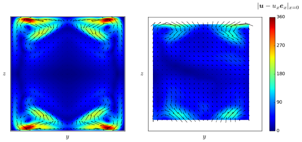
Figure 8: Velocity distribution of the secondary flow ($u_{y}\boldsymbol{e}_{y}+u_{z}\boldsymbol{e}_{z})|_{x=0}$ for $Ta=10^{5}$ (left: computed steady state from the numerical simulation, right: measured mean values)

A corresponding comparison of numerical simulation and experiment with respect to the secondary flow can be found in Fig. 8 showing the flow pattern in the meridional plane $x=0$ for $Ta=10^{5}$. Due to the saturation effects described above, the measurement system does not provide valid velocity measurements near the walls. Unfortunately, the secondary flow shows the most striking structures and maximum values just in regions near the top and the bottom of the container, which are out of the UADV measuring domain. The numerical results reveal the existence of distinct vortex pairs which are driven by Ekman pumping in the top and bottom boundary layers.

In order to validate the numerical scheme we compared the numerical results and the measured experimental data with respect to both the velocity profiles and the integral quantities as the kinetic energy of the secondary flow. Figure 9 presents an example of a mean profile of the velocity component $u_{x}$ along the line $x=0.637,-1<y<1,z=0$ for $Ta=10^{5}$.

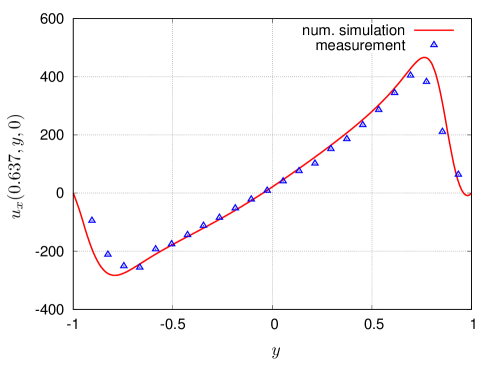
Figure 9: Mean measured profile of the velocity component $u_{x}$ (blue points) and corresponding numerical simulation profile (red line) along the line $x=0.637,-1<y<1,z=0$ for $Ta=10^{5}$.

IV.2 Transition to unsteady flow regimes

In order to assess the critical Taylor number $Ta_{c}$ for the transition from laminar to oscillatory or unsteady flow regimes, we consider the time evolution of the velocity field during the spin-up process where the flow field is evolving from the state of rest after a sudden start-up of the RMF.

Fig. 10 displays the time evolution of the kinetic energy of the primary flow

$$<u_{x}^{2}+u_{y}^{2}>|_{z=0}=\frac{1}{N_{x}N_{y}}\sum_{i,j}^{N_{x},N_{y}}{u_{x}}_{ij}^{2}+{u_{y}}_{ij}^{2}$$ (12)

in the middle horizontal plane $z=0$ for $Ta=10^{5}$.

The so-called spin-up time $t_{spin-up}=2H/\sqrt{\nu\Omega_{ce}}\propto Ta^{-1/3}$ is utilized to analyze spin-up dynamics of a melt driven by RMF in a circular cylindrical container Ungarish (1997); Nikrityuk et al. (2005). $\Omega_{ce}$ denotes the effective steady-state angular velocity at the center. Using the expression (16) given by Nikrityuk Nikrityuk et al. (2005) and applying it for $Ta=10^{5}$ we obtain: $t_{spin-up}=0.0542$, which is indicated for comparison in Fig. 10.

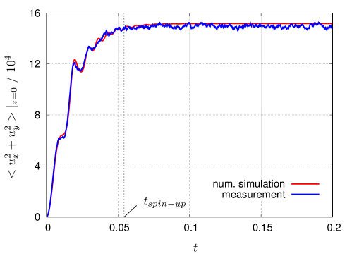
Figure 10: Spin-up of the kinetic energy of the primary flow $<u_{x}^{2}+u_{y}^{2}>$ at the middle horizontal plane $z=0$ for $Ta=10^{5}$ (blue: measured and red: values computed from the numerical simulation). $t_{spin-up}$ denotes the so-called spin-up time as defined by Nikrityuk et al. Nikrityuk et al. (2005) for RMF driven flows in a circular cylindrical container.

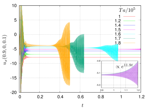
Figure 11: Simulation: Time evolution of the velocity component $u_{x}$ at the monitoring point $x=0.9,y=0,z=0.1$ for different values of the Taylor number $Ta$ showing the characteristic exponential growth of the first emerging flow instabilities.

Fig. 11 shows numerical results with respect to the time evolution of the velocity component $v_{x}$ at a monitoring point with the coordinates $x=0.9,y=0,z=0.1$ for different values of the magnetic Taylor number $Ta$.

The initial state is dominated by inertial oscillations which are forced by the rapid increase in the rotation rate. Because of viscous damping, these oscillations decay and can be observed therefore only during a finite initial time period which roughly corresponds to the spin-up time  Nikrityuk et al. (2005); Räbiger, Eckert, and Gerbeth (2010). Finally, the flow reaches a steady state. The transition to a time-dependent flow regime becomes obvious by a reappearance of pronounced oscillations of the velocity signal. Figure 11 demonstrates the exponential growth of the instabilities. In this figure the drawings of the velocity curves for each Taylor number are terminated at the time, where the saturation was achieved after the exponential growth phase. We will discuss different transition phases later in this section in more detail (see Fig. 14). For $Ta=1.6\times 10^{5}$ we detected using a proper orthogonal decomposition (see Sec. IV.3) for the first upcoming instability a growth rate of $\approx 20.5$ and afterwards a phase with velocity oscillations having the period of $\approx 0.00345$.

The transition from a steady to a time-dependent flow regime was observed for magnetic Taylor numbers being larger as a minimum value in the range of $1.2\times 10^{5}<Ta_{c}<1.3\times 10^{5}$. The corresponding critical value for the case of a finite circular cylinder of aspect ratio 1 is $Ta_{c}=1.232\times 10^{5}$ given by Grants et al. Grants and Gerbeth (2001).

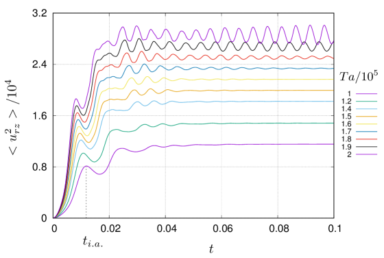
Figure 12: Simulation: Time evolution of the mean kinetic energy of the secondary flow (c.f. Eq. 13). The time required for achieving the first maximum is called initial adjustment time $t_{i.a}$.

Fig. 12 depicts the time evolution of the over the whole volume averaged kinetic energy of the secondary flow

$$<u_{rz}^{2}>=\frac{1}{V}\int dV\,(u_{r}^{2}+u_{z}^{2})\,,$$ (13)

where $u_{r}=u_{x}cos(\varphi)+u_{y}sin(\varphi)$ is the radial velocity component in polar coordinates.

The behaviour shown here appears to be similar as reported for the case of the RMF-driven flow in a finite cylinder Räbiger, Eckert, and Gerbeth (2010); Nikrityuk et al. (2005); Ungarish (1997).

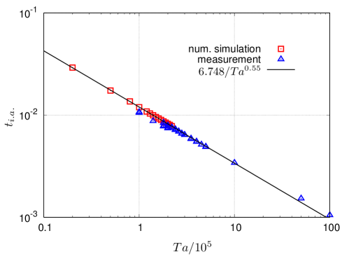
Figure 13: Initial adjustment time $t_{i.a.}$ as a function of the Taylor number $Ta$.

The time between initiating the magnetic field and reaching the first maximum of the energy amplitude is the so-called initial adjustment time $t_{i.a.}$ Nikrityuk et al. (2005). In Fig. 13 the initial adjustment time is drawn as a function of the Taylor number $Ta$. The expression $t_{i.a.}=6.748/Ta^{0.54}$ describes very good this relationship.

For Taylor numbers just above the critical value, i.e. for $Ta<1.4\times 10^{5}$, the numerical simulations reveal a convergence of the flow to a stationary state. A further increase of the magnetic Taylor number leads to oscillatory flow regimes which characteristic frequencies depend on the magnetic Taylor number $Ta$ and the time passed since the initial adjustment time $t_{i.a.}$, respectively. Fig. 14 helps to clarify these situations.

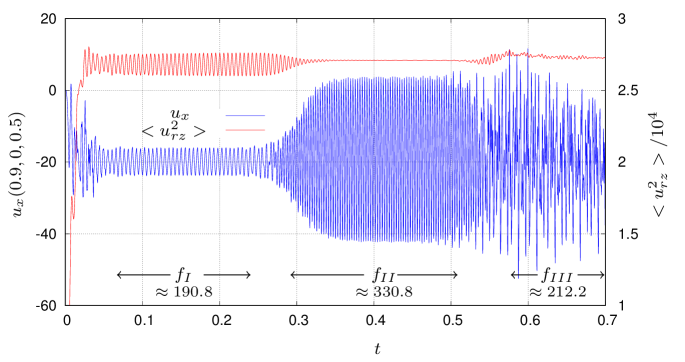
Figure 14: Simulation: Time evolution of the kinetic energy of the secondary flow (red) and of the velocity component $u_{x}$ at the monitoring point with the coordinates $(0.9,0,0.5)$ (blue) for $Ta=1.9\times 10^{5}$ showing three characteristic oscillation frequencies ($f_{I}$, $f_{II}$ and $f_{III}$) occurring at three different time intervals, respectively.

Fig. 14 presents both the time evolution of the volume averaged kinetic energy of the secondary flow $<u^{2}_{rz}>$ (c.f. Eq. 13) and the velocity component $u_{x}$ at the monitoring point $P=(0.9,0,0.5)$ for $Ta=1.9\times 10^{5}$. Unlike as in Fig. 11 here we also show the flow behaviour beyond the onset of the saturation phase. We can recognize three different oscillatory regimes at different moments in time showing unique characteristic frequencies in each case, namely: $f_{I}$, $f_{II}$ and $f_{III}$ for the time intervals: $0.06<t<0.25$, $0.3<t<0.5$ and $0.58<t$, respectively. The successive appearance of different frequencies is closely related to the transient behaviour of different flow modes. This can be studied in detail by a proper orthogonal decomposition, which will be presented in section IV.3.

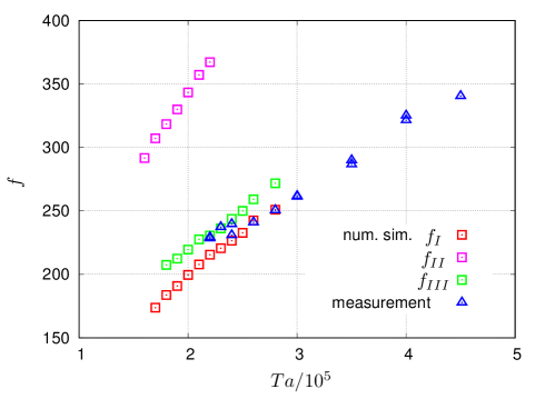
Figure 15: Characteristic oscillation frequencies of the secondary flow in the plane $x=0$ as a function of the Taylor number $Ta$ showing three different branches: $f_{I},f_{II}$ and $f_{III}$ which appears at different time intervals during the evolution of the flow (see Fig. 14).

In order to quantify the oscillating behaviour of the flow a discrete Fourier analysis of the kinetic energy of the secondary flow was performed. Fig. 15 shows the characteristic oscillation frequencies of the secondary flow velocity as a function of the Taylor number $Ta$ in the range $Ta_{1}=1.5\times 10^{5}<Ta<Ta_{2}=4.5\times 10^{5}$ comparing the experimental results and those derived from the numerical simulation. Here, too, a very good agreement between the measurements and the numerical calculations can be noticed.

The frequency domain $f_{I}$ corresponds to flow oscillations, which occur directly after the spin-up phase. The branch $f_{III}$ corresponds to the flow oscillations in the asymptotic phase, which is the time period after completing the spin-up phase, when all growing modes have been evolved.

Our analysis revealed that the flow structure has a periodic character in the range $Ta_{1}=1.5\times 10^{5}<Ta<Ta_{2}=4.5\times 10^{5}$. The specific case $Ta=2.6\times 10^{5}$ was selected for further examination. We applied a discrete Fourier analysis of the velocity data to determine the peak frequency. For the numerical data a value of $f_{I}=242.5$ was found corresponding to a period of $T\approx 0.00412$. Fig. 16 shows four snapshots of the secondary flow (contour plots of $\sqrt{(u_{y}^{2}+u_{z}^{2})}|_{x=0}$) for $Ta=2.6\times 10^{5}$. The numerically predicted flow structure of the secondary flow is well confirmed by corresponding velocity measurements on the plane $x=0$ which are displayed in Fig. 17. A Fourier analysis of the measurements resulted in a peak frequency of $f=241$ corresponding to a period of $T\approx 4.15\times 10^{-3}$. The sampling interval was $\Delta t=9.356\times 10^{-5}$ ($\Delta t={0.3126}\,\mathrm{s}$ in physical units). We can recognize, that the flow structure has a periodic character with the period $44\times\Delta t=4.12\times 10^{-3}$, which corresponds very well with the data coming from the numerical simulation for the same Taylor number (cf. Fig. 16).

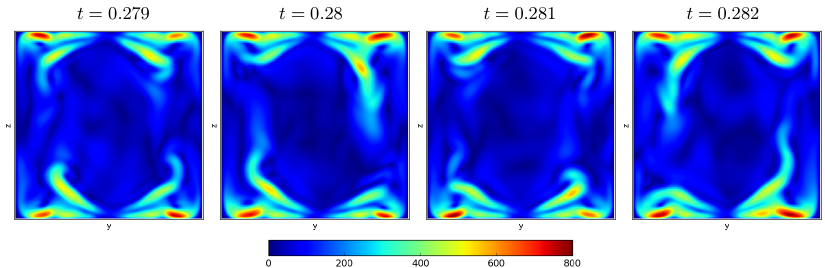
Figure 16: Simulation: Snapshots of the secondary flow (contour plots of $\sqrt{(u_{y}^{2}+u_{z}^{2})}|_{x=0}$) for $Ta=2.6\times 10^{5}$.

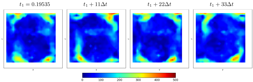
Figure 17: Measured snapshots of the secondary flow (contour plots of $\sqrt{u_{y}^{2}+u_{z}^{2}}$) for $Ta=2.6\times 10^{5}$ showing the periodic character of the flow. The sampling interval was $\Delta t=9.356\times 10^{-5}$.

In order to ensure mesh refinement independence, convergence studies at different typical regimes were carried out. For instance, at $Ta=10^{5}$ (steady flow regime) and at $Ta=1.9\times 10^{5}$ (oscillatory flow regime showing 3 different transient intervals with 3 different oscillatory frequencies, respectively). Table 1 gives the mean steady state secondary flow velocity for $Ta=10^{5}$ and the three characteristic oscillation frequencies for $Ta=1.9\times 10^{5}$ depending of the mesh refinement.

	mesh I	mesh II	mesh III	mesh IV
number of cells	$10^{6}$	$1.57\times 10^{6}$	$2\times 10^{6}$	$2.46\times 10^{6}$
$Ta=10^{5}$
$<u_{rz}>^{1/2}$	107.24	107.39	107.47	107.51
$Ta=1.9\times 10^{5}$
$f_{I}$	189.3	190.4	190.8	190.3
$f_{II}$	328.5	329.5	330.8	330.2
$f_{III}$	219.1	216.5	212.2	214.5

Table 1: Steady state secondary flow velocity for $Ta=10^{5}$ and characteristic oscillation frequencies at different transient flow regimes for $Ta=1.9\times 10^{5}$ depending of the mesh refinement.

A characteristic of the spin-up is $t_{99}$, which denotes the time from the onset of the magnetic field to the moment the primary flow reaches 99 percent of the steady state velocity. It is worth to mention, that both, $t_{spin-up}$ and $t_{99}$, are almost identical in a broad range of the Taylor number below the critical Taylor number $Ta_{c}$ but they show different scaling behaviours with respect to the Taylor number $Ta$ (c.f. Table 2 eqn. 14).

Fig. 18 shows the time evolution of the volume averaged azimuthal velocity component $<u_{\varphi}>=1/V~{}\int dV~{}u_{\varphi}$ using suitable scales. Within this representation, the time evolution of $u_{\varphi}$ for different value of the Taylor number collapse to one curve. The following scaling laws can be compiled for the interval $10^{4}<Ta<1.6\times 10^{5}$:

$$t_{99}\approx 1.036~{}Ta^{-1/4},\quad<u_{\varphi}>\approx 0.1475~{}Ta^{2/3}\quad\mbox{and}\quad\Omega\approx 0.167~{}Ta^{3/4}\,.$$ (14)

Here is $\Omega=(u_{\varphi}(x,y,0)/r)|_{r\to 0}$ the core rotation speed, which is defined as the angular velocity at half height of the vertical center axis.

$Ta$	$t_{i.a.}$	$t_{99}$	$t_{spin-up}$	$\displaystyle\frac{t_{99}}{t_{spin-up}}$	$<u_{\varphi}>|_{t\to\infty}$	$\Omega$
$10^{4}$	0.0436	0.1145	0.1168	1.02	65.86	155.4
$2\times 10^{4}$	0.0292	0.0922	0.0927	1	108.5	269.8
$5\times 10^{4}$	0.0174	0.07	0.0683	0.976	202.6	551
$8\times 10^{4}$	0.0136	0.0615	0.0584	0.95	275.8	793.2
$10^{5}$	0.01196	0.058	0.0542	0.935	318.9	942
$1.2\times 10^{5}$	0.01085	0.05575	0.051	0.915	359	1082

Table 2: Characteristic time scales, mean azimuthal velocity and core rotation speed for different values of the Taylor number $Ta$.

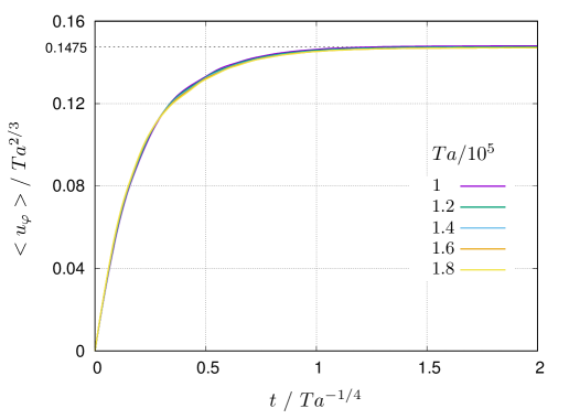
Figure 18: Simulation: Time evolution of the volume averaged azimuthal velocity $<u_{\varphi}>$ using the scales $Ta^{2/3}$ for the velocity and $Ta^{-1/4}$ for the time, respectively.

IV.3 Proper Orthogonal Decomposition (POD)

The proper orthogonal decomposition (POD) is a powerful method for data analysis aimed at obtaining low-dimensional approximate descriptions of complex flows using a model reduction. This technique provides a basis for the modal decomposition of data recorded in the course of experiments or numerical simulations. The POD decomposes the vector flow field into orthogonal spatial modes and time-dependent amplitudes. For a detailed description of POD applications in the field of computational fluid dynamics the reader is referred to Holmes et al. Holmes, Lumley, and Berkooz (1998). In general, a velocity field $\boldsymbol{u}(\boldsymbol{x},t)$ can be considered as the sum of a steady mean flow $\boldsymbol{u}_{0}(\boldsymbol{x})$ and a fluctuating part $\boldsymbol{u}^{*}(\boldsymbol{x},t)$:

$$\boldsymbol{u}(\boldsymbol{x},t)=\boldsymbol{u}_{0}(\boldsymbol{x})+\boldsymbol{u}^{*}(\boldsymbol{x},t)\,.$$ (15)

The fluctuating velocity field $\boldsymbol{u}^{*}(\boldsymbol{x},t)$ is decomposed into a sum of a limited number of proper modes

$$\boldsymbol{u}^{*}(\boldsymbol{x},t)=\sum_{m=1}^{N_{m}}u^{*}_{m}(\boldsymbol{x},t)=\sum_{m=1}^{N_{m}}a_{m}(t)\varphi_{m}(\boldsymbol{x})\,,$$ (16)

where the $N_{m}$ functions $\varphi_{m}(\boldsymbol{x})$ provide the orthogonal basis and the time dependency is represented by the respective amplitudes $a_{m}(t)$. Minimizing the projection error is equivalent to achieving an optimal description of the kinetic energy.

In this study, we use the snapshot method which discretizes the distribution of the velocity variations $\boldsymbol{u}^{*}$ in space and time:

$$\boldsymbol{u}_{ij}=\boldsymbol{u}^{*}(\boldsymbol{x}_{i},t_{j})\,,\qquad\mbox{with}\quad i=1,...,N_{x}\quad\mbox{and}\quad j=1,...,N_{t}.$$ (17)

$\boldsymbol{x}_{i}$ are the center coordinates of the finite volumes, in which the spatial domain is sub-divided. Now we can write the POD (Eq. 16) in a discrete notation:

$$\boldsymbol{u}_{ij}=\sum_{m=1}^{N_{m}}a_{mj}\boldsymbol{\varphi}_{im}\,,\qquad\mbox{with}\quad a_{mj}=a_{m}(t_{j})\quad\mbox{and}\quad\boldsymbol{\varphi}_{im}=\boldsymbol{\varphi}_{m}(\boldsymbol{x}_{i})\,.$$ (18)

The functions $\boldsymbol{\varphi}_{m}(\boldsymbol{x})$ constitute an orthogonal basis with the inner product defined as

$$<\boldsymbol{\varphi}_{m}|\boldsymbol{\varphi}_{n}>=\sum_{i=1}^{N_{x}}\varphi_{im}W_{i}\varphi_{in}=\delta_{mn}\,,$$ (19)

where $W_{i}$ are weight functions being necessary for taking into account the significance of the different contributions by regions of the spatial discretization with different volumes. In our analysis we used the weight functions $W_{i}=v_{i}/v_{max}$ as the ratio of the specific cell volume $v_{i}$ with respect to the maximum cell volume $v_{max}$.

The parallelized Python library modred was applied for model reduction, modal analysis, and system identification of large systems and datasets as described in Belson, Tu, and Rowley (2014). The routine modred.compute_POD_matrices_snap_method returns the modes $\boldsymbol{\varphi}_{m}$ and the eigenvalues $\lambda_{m}$ of the snapshot correlation matrix starting with the snapshots $\boldsymbol{u}_{ij}$, which can be expressed as time integral of the kinetic energy of mode $m$:

$$\lambda_{m}=\int dt<u_{m}^{*}|u_{m}^{*}>=\sum_{j}a_{mj}^{2}\,.$$ (20)

The modes are sorted in such a way, that $\lambda_{1}>\lambda_{2}>\lambda_{3}>...>\lambda_{N_{m}}$.

In order to evaluate the contribution rate of the mode $m$ to total kinetic energy of the system, the normalized energy fraction

$$E_{m}=\frac{\lambda_{m}}{\sum_{k=1}^{N_{m}}\lambda_{k}}$$ (21)

has been used throughout the paper.
POD of a slightly supercritical flow
At first we consider a slightly supercritical flow occurring at $Ta=1.7\times 10^{5}>Ta_{c}$. To study the structure and time-dependent behaviour of the flow for this value of the Taylor number we use the data obtained by numerical simulations only.

We begin with the proper orthogonal decomposition of the numerical simulation data and particularly with the data of the primary flow. i.e. the velocity distribution on the horizontal plane $z=0$.

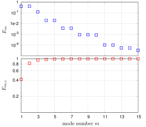
Figure 19: POD of the numerical simulation data of the primary flow for $Ta=1.7\times 10^{5}$ - Contribution of each particular mode to the total kinetic energy (top) and cumulative energy fraction $E_{m,c}=\sum_{k=1}^{m}E_{k}$ (bottom).

The POD of the numerical data has been performed starting at the non-dimensional time $t=0.3$ in order to skip the spin-up phase. Fig. 19 shows the contribution of the first 15 most important modes to the total kinetic energy. It becomes apparent that mode $1$ and modes $2$ have the same integral kinetic energy. Moreover, both modes show similar flow structures (cf. Fig. 21). We can see in Fig. 19 that the first $5$ modes contain already $98.9\%$ of the total kinetic energy of the primary flow.

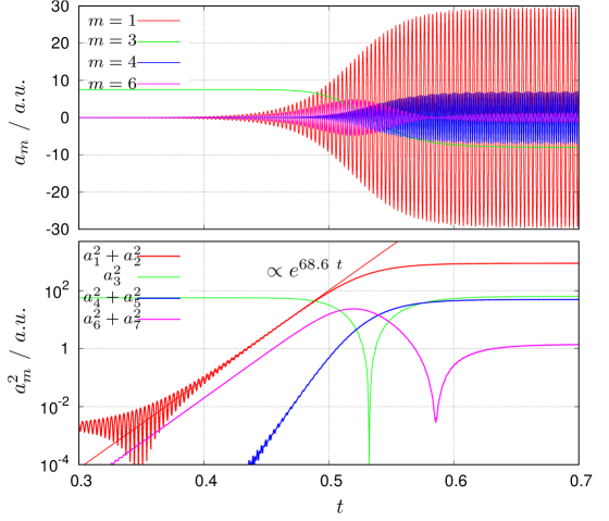
Figure 20: POD of the primary flow (numerical simulation for $Ta=1.7\times 10^{5}$) - Time evolution of the amplitude of the most important modes $a_{m}(t);m=1,3,4,6$ (top) and of the kinetic energy of the modes $m=1,...,7$ (bottom).

Fig. 20 depicts the time evolution of the amplitudes of the leading modes $a_{1}(t),a_{3}(t),a_{4}(t)$ and $a_{6}(t)$. The upper diagram demonstrates the exponential growth of the modes whereas the evolution of the kinetic energy $a_{m}(t)^{2}$ of the modes $m=1,2,...,7$ can be seen in the bottom graph.

We can recognize that the kinetic energy of the modes $1$ and $2$ grow exponentially with the growth rate $g.r._{1,2}=68.6$. Using a discrete Fourier transform we determined the oscillating frequency of the amplitude $a_{1}(t)$ to be $f_{1}=306$.

Table 3 shows the growth rate of the most important POD mode of a slightly supercritical flow for different values of the Taylor number. An extrapolation of these values towards zero results in a critical Taylor number of $Ta_{c}\approx 1.26\times 10^{5}$.

$Ta$	$1.5\times 10^{5}$	$1.6\times 10^{5}$	$1.7\times 10^{5}$	$1.8\times 10^{5}$
$g.r.$	11.9	20.5	34.3	48.6

Table 3: Growth rate of the most important POD mode of a slightly supercritical flow for different values of the Taylor number.

Fig. 21 displays vector plots of the mean flow and the horizontal projection of the mode functions in the horizontal plane $z=0$, i.e. $(\boldsymbol{\varphi}_{m}-\boldsymbol{\varphi}_{m}\cdot\boldsymbol{e}_{z})(x,y,z=0)$ (primary flow), for the first $5$ leading modes. We can observe, that the modes $(1,2)$ and $(4,5)$ appear pairwise showing similar structures and the same kinetic energy, respectively. While these modes can be related to differential rotation of the flow in the horizontal cross section, mode 3 represents the transient behaviour of the small counter-rotating vortices in the corners.

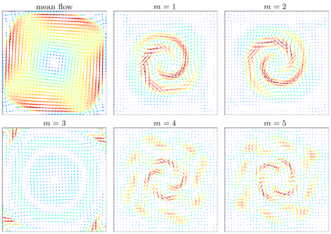
Figure 21: Simulation: POD - Velocity vector plot of the horizontal projection $\boldsymbol{\varphi}_{m}-\boldsymbol{\varphi}_{m}\cdot\boldsymbol{e}_{z}$ of the mode functions at the horizontal plane $z=0$ (primary flow, $Ta=1.7\times 10^{5}$)

For a better understanding of the three-dimensional structure of the principal unstable flow modes, we show in Fig 22 isosurfaces of $\Lambda_{2}$, the second largest eigenvalue of the sum of the square of the symmetrical and anti-symmetrical parts of the velocity gradient tensor for $Ta=1.7\times 10^{5}$. The $\Lambda_{2}$ vortex criterion can adequately identify vortices from a three-dimensional velocity field Jeong and Hussain (1995).

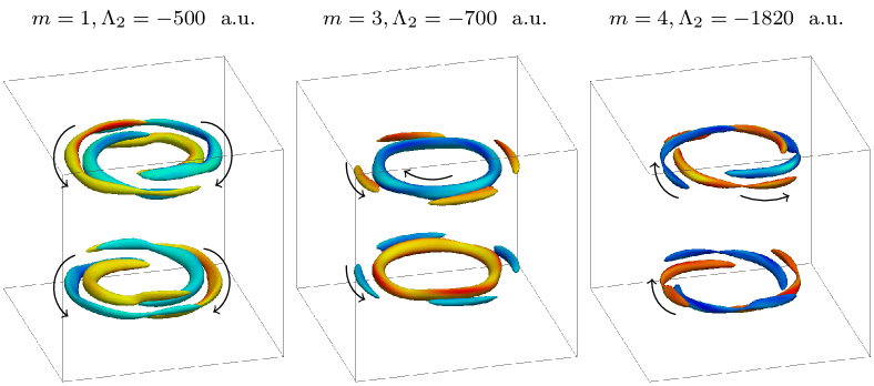
Figure 22: Simulation: Isosurfaces of $\Lambda_{2}$, the second largest eigenvalue of the sum of the square of the symmetrical and anti-symmetrical parts of the velocity gradient tensor for the most important modes $m=1$, $m=3$ and $m=4$ ($Ta=1.7\times 10^{5}$). The color indicates the sign of azimuthal vorticity and the arrows shows the direction of the azimuthal velocity.

The structures shown in Fig. 22 form pairs or quartets of counter-rotating tubes. These vortices are responsible for the velocity fluctuations observed in Fig. 20 and for the symmetry breaking of the basic steady flow. The red curve there corresponds to the time evolution of the mode $m=1$ and the blue curve corresponds to the mode $m=4$.

In Sec. IV.2, we have seen, that the experimental data show an oscillating behaviour, especially for the case of the secondary flow. In analogy to the numerical simulation, we perform a proper orthogonal decomposition of the measurement data for supercritical flows to characterize the secondary flow.
POD of a supercritical flow
In order to obtain a good basis for the comparison between the numerical simulations and the experimental data, we consider in both cases the primary and the secondary flow together as one item during the POD processing. For $Ta<2.2\times 10^{5}$ we cannot identify in the measurements any characteristic flow frequencies (see Fig. 15). Therefore, the POD analysis was conducted for a Taylor number of $Ta=2.6\times 10^{5}$, which is approximately two times the critical value $Ta_{c}$.

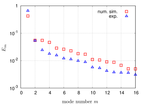
Figure 23: POD of the numerical (red) and experimental data (blue) of the secondary flow - Contribution of each particular mode to the total kinetic energy for $Ta=2.6\times 10^{5}$

Fig. 23 shows the contribution to the kinetic energy of each mode and Fig. 24 shows the time evolution of both the amplitude of the first important modes $a_{m}(t)$ (top) and the corresponding kinetic energies (bottom) of the experimental data coming from the measurements of both the primary and the secondary flow for $Ta=2.6\times 10^{5}$. The amplitude of the first important mode $m=1$ decreases during the spin-up phase and reveals the same structure as those for the mean flow. (see Fig. 24) The amplitude of the second mode increases exponentially and shows an oscillatory behaviour in the saturation phase for $t>0.2$.

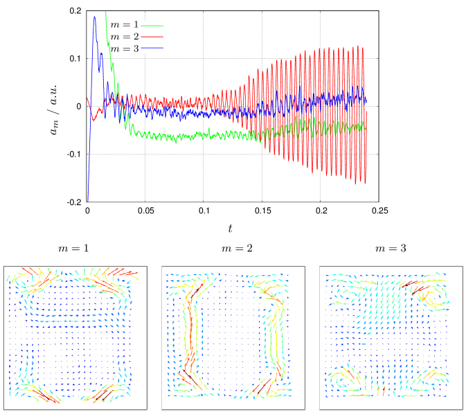
Figure 24: POD of the experimental data - Time evolution of the amplitude of the first important modes $a_{m}(t)$ (top) and corresponding modes flow structures of the secondary flow (bottom) for $Ta=2.6\times 10^{5}$

Fig. 24 shows the structure of the most important modes of the secondary flow for $Ta=2.6\times 10^{5}$. These results confirm very well the corresponding findings from the numerical simulations, which are shown in Fig. 25.

Figure 25 shows the POD of the numerical simulation for $Ta=2.6\times 10^{5}$, which corresponds to Figs. 24 coming from the experiments for the same value of the Taylor number. We can identify that the combination of the modes $m=2$ and $m=3$ grows exponentially and shows the same structure as the experimental mode $m=2$. Obviously, this pattern is equivalent to a recirculation roll covering the vertical section of the cube. The instability revealed in the Figs. 16 and 17 is related to this mode. The mode $m=1$ describes in both cases the initial spin-up phase of the flow and has exactly the same structure as the mean flow but with opposite sign.

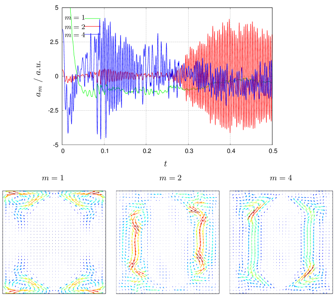
Figure 25: POD of the numerical simulation - flow structure of the most important modes of the secondary flow for $Ta=2.6\times 10^{5}$

V Conclusions

Numerical simulations and experimental investigations were performed within this study for investigating characteristic flow patterns arising in an electrically conducting fluid inside a closed cubic container in consequence of the applying a rotating magnetic field. Direct numerical simulations were performed using a semi-analytical expression for the induced electromagnetic force density. Two-dimensional distributions of the fluid velocity in two perpendicular planes were measured by means of a dual-plane two-component ultrasound array Doppler velocimeter (UADV) with a high frame rate. It was demonstrated that this instrumentation allows for reliable and accurate measurements of very small velocities in the laminar regime ($\leq{1}\,\mathrm{mm/s}$), but, can also resolve the time-dependent flow in the turbulent region, where the velocity can achieve values of several cm/s. Due to the non-deterministic onset of oscillatory instabilities, multi-plane flow imaging with a high frame rate over long durations is crucial to capture the flow spanning multiple time scales. This requirement is met by the UADV system by real-time data compression on an FPGA and continuous streaming. We performed UADV measurements with a frame rate up to $f=11.2~{}Hz$ an a duration of up to $5000~{}s$.

Our results reveal that the fluid flow observed inside the cube shows a remarkable resemblance to the flow structures occurring in a circular cylinder. In particular, we found the transition from the steady state to time dependent flow structures at a critical $Ta$ number at $Ta_{c}>1.26\times 10^{5}$ ($Ta_{c}=1.232\times 10^{5}$ for a cylinder with aspect ratio 1). With respect to the scaling behaviour of the primary flow intensity we obtained a relationship for small values of the Taylor number ($Ta<2\times 10^{2}$) corresponding to $Re_{max}\approx 0.031~{}Ta$ and $Re_{max}\approx 2.08~{}Ta^{1/2}$ for high Ta numbers ($Ta>4\times 10^{5}$), respectively. Both scaling laws assort well with either analytical relations or predictions made by Davidson and Hunt Davidson and Hunt (1987) for the case of an RMF-driven flow in an infinite circular cylinder.

The occurrence and exponential growth of spontaneous flow instabilities was observed numerically and in the experiment. The characteristic frequencies of the oscillating flow just above the critical Taylor number $Ta_{c}$ were determined. The POD method was applied to identify the dominating modes of the flow structure. Unlike the case of the RMF-driven flow in a circular cylinder, we did not find Taylor - Görtler vortices neither in the numerical simulation nor in the experiments. The absence of curved walls in the cube might be the reason for this difference. Numerical simulations and flow measurements show an excellent agreement and provide accurate results with respect to both the mean flow structures and the evolution of the flow in time.

References

- Gerbeth, Eckert, and Odenbach (2013) G. Gerbeth, K. Eckert, and S. Odenbach, “Electromagnetic flow control in metallurgy, crystal growth and electrochemistry,” The European Physical Journal Special Topics 220, 1 – 8 (2013).
- Davidson and Hunt (1987) P. A. Davidson and J. C. R. Hunt, “Swirling recirculation flow in a liquid-metal column generated by a rotating magnetic field,” Journal of Fluid Mechanics 185, 67–106 (1987).
- Gelfgat, Grants, and Priede (1995) Y. M. Gelfgat, I. Grants, and J. Priede, “Mhd flow in flat layers in rotating and constant magnetic fields,” Magnetohydrodynamics 31, 125 – 133 (1995).
- Barz et al. (1997) R. Barz, G. Gerbeth, U. Wunderwald, E. Buhrig, and Y. Gelfgat, “Modelling of the isothermal melt flow due to rotating magnetic fields in crystal growth,” Journal of Crystal Growth 180, 410 –421 (1997).
- Kaiser and Benz (1998) T. Kaiser and K. W. Benz, “Taylor vortex instabilities induced by a rotating magnetic field: A numerical approach,” Physics of Fluids 10, 1104 –1110 (1998).
- Witkowski, Walker, and Marty (1999) L. M. Witkowski, J. S. Walker, and P. Marty, “Nonaxisymmetric flow in a finite-length cylinder with a rotating magnetic field,” Physics of Fluids 11, 1821 – 1826 (1999).
- Grants and Gerbeth (2001) I. Grants and G. Gerbeth, “Stability of axially symmetric flow driven by a rotating magnetic field in a cylindrical cavity,” Journal of Fluid Mechanics 431, 407–426 (2001).
- Grants and Gerbeth (2002) I. Grants and G. Gerbeth, “Linear three-dimensional instability of a magnetically driven rotating flow,” Journal of Fluid Mechanics 463, 229 – 239 (2002).
- Grants and Gerbeth (2003) I. Grants and G. Gerbeth, “Experimental study of non-normal non-linear transition to turbulence in a rotating magnetic field driven flow,” Physics of Fluids 15, 2803 – 2809 (2003).
- Ungarish (1997) M. Ungarish, “The spin-up of liquid metal driven by a rotating magnetic field,” Journal of Fluid Mechanics 347, 105 – 118 (1997).
- Nikrityuk et al. (2005) P. A. Nikrityuk, M. Ungarish, K. Eckert, and R. Grundmann, “Spin-up of a liquid metal flow driven by a rotating magnetic field in a finite cylinder: A numerical and an analytical study,” Physics of Fluids 17, 067101 (2005).
- Räbiger, Eckert, and Gerbeth (2010) D. Räbiger, S. Eckert, and G. Gerbeth, “Measurements of an unsteady liquid metal flow during spin-up driven by a rotating magnetic field,” Experiments in Fluids 48, 233 – 244 (2010).
- Vogt et al. (2012) T. Vogt, I. Grants, D. Räbiger, S. Eckert, and G. Gerbeth, “On the formation of taylor-görtler vortices in rmf-driven spin-up flows,” Experiments in Fluids 52, 1 – 10 (2012).
- Dubke et al. (1988a) M. Dubke, K.-H. Tacke, K.-H. Spitzer, and K. Schwerdtfeger, “Flow fields in electromagnetic stirring of rectangular strands with linear inductors: Part i. theory and experiments with cold models,” Metallurgical Transactions B 19, 581 – 593 (1988a).
- Dubke et al. (1988b) M. Dubke, K.-H. Tacke, K.-H. Spitzer, and K. Schwerdtfeger, “Flow fields in electromagnetic stirring of rectangular strands with linear inductors: Part ii. computation of flow fields in billets, blooms, and slabs of steel,” Metallurgical Transactions B 19, 595 – 602 (1988b).
- Frana and Stiller (2008) K. Frana and J. Stiller, “A numerical study of flows driven by a rotating magnetic field in a square container,” European Journal of Mechanics - B/Fluids 27, 491 – 500 (2008).
- Pal et al. (2009) J. Pal, A. Cramer, T. Gundrum, and G. Gerbeth, “Multimag—a multipurpose magnetic system for physical modelling in magnetohydrodynamics,” Flow Measurement and Instrumentation 20, 241 – 251 (2009).
- Takeda (1991) Y. Takeda, “Development of an ultrasound velocity profile monitor,” Nuclear Engineering and Design 126, 277 – 284 (1991).
- Franke et al. (2010) S. Franke, L. Büttner, J. Czarske, and S. E. D. Räbiger, “Ultrasound doppler system for two-dimensional flow mapping in liquid metals,” Flow Measurement and Instrumentation 21, 402 – 409 (2010).
- Nauber et al. (2013) R. Nauber, M. Burger, L. Büttner, S. Franke, D. Räbiger, S. Eckert, and J. Czarske, “Novel ultrasound array measurement system for flow mapping of complex liquid metal flows,” The European Physical Journal 220, 43 – 52 (2013).
- Franke et al. (2013) S. Franke, H. Lieske, A. Fischer, L. Büttner, J. Czarske, D. Räbiger, and S. Eckert, “Two-dimensional ultrasound doppler velocimeter for flow mapping of unsteady liquid metal flows,” Ultrasonics 53, 691–700 (2013).
- Kasai et al. (1985) C. Kasai, K. Namekawa, A. Koyano, and R. Omoto, “Real-time two-dimensional blood flow imaging using an autocorrelation technique,” , IEEE Transactions on Sonics and Ultrasonics 32, 458 – 464 (1985).
- Nauber et al. (2016) R. Nauber, N. Thieme, H. Radner, H. Beyer, L. Büttner, K. Dadzis, O. Pätzold, and J. Czarske, “Ultrasound flow mapping of complex liquid metal flows with spatial self-calibration,” Flow Measurement and Instrumentation 48, 59 –63 (2016).
- OpenCFD (2015) OpenCFD, OpenFOAM - The Open Source CFD Toolbox - User’s Guide, OpenCFD Ltd., United Kingdom, 3rd ed. (2015).
- Issa (1986) R. I. Issa, “Solution of the implicitly discretised fluid flow equations by operator-splitting,” Journal of computational physics 62, 40–65 (1986).
- Ferziger and Peric (2003) J. Ferziger and M. Peric, Computational Methods for Fluid Dynamics (Springer Berlin Heidelberg, 2003).
- Plevachuk et al. (2014) Y. Plevachuk, V. Sklyarchuk, S. Eckert, G. Gerbeth, and R. Novakovic, “Thermophysical properties of the liquid ga−in−sn eutectic alloy,” Journal of Chemical and Engineering Data 59, 757 – 763 (2014).
- Holmes, Lumley, and Berkooz (1998) P. Holmes, J. Lumley, and G. Berkooz, Turbulence, Coherent Structures, Dynamical Systems and Symmetry, Cambridge Monographs on Mechanics (Cambridge University Press, 1998).
- Belson, Tu, and Rowley (2014) B. A. Belson, J. H. Tu, and C. W. Rowley, “Algorithm 945: Modred - A parallelized model reduction library,” ACM Transactions on Mathematical Software 40, 30:1–30:23 (2014).
- Jeong and Hussain (1995) J. Jeong and F. Hussain, “On the identification of a vortex,” Journal of Fluid Mechanics 285, 69–94 (1995).