Dynamical scaling for underdamped strain order parameters
quenched below first-order phase transitions

N. Shankaraiah, Awadhesh K. Dubey, Sanjay Puri and Subodh R. Shenoy School of Physical Sciences, Jawaharlal Nehru University, New Delhi 110067, India;
TIFR Centre for Interdisciplinary Sciences, TIFR Hyderabad 500075, India.
Abstract

In the conceptual framework of phase ordering after temperature quenches below transition, we consider the underdamped Bales-Gooding-type ’momentum conserving’ dynamics of a 2D martensitic structural transition from a square-to-rectangle unit cell. The one-component or NOP=1subscript𝑁OP1N_{\rm OP}=1 order parameter is one of the physical strains, and the Landau free energy has a triple well, describing a first-order transition. We numerically study the evolution of the strain-strain correlation, and find that it exhibits dynamical scaling, with a coarsening length L(t)tαsimilar-to𝐿𝑡superscript𝑡𝛼L(t)\sim t^{\alpha}. We find at intermediate and long times that the coarsening exponent sequentially takes on respective values close to α=2/3𝛼23\alpha=2/3 and α=1/2𝛼12\alpha=1/2. For deep quenches, the coarsening can be arrested at long times, with α0similar-to-or-equals𝛼0\alpha\simeq 0. These exponents are also found in 3D. To understand such behaviour, we insert a dynamical-scaling ansatz into the correlation function dynamics to give, at a dominant scaled separation, a nonlinear kinetics of the curvature g(t)1/L(t)𝑔𝑡1𝐿𝑡g(t)\equiv 1/L(t). The curvature solutions have time windows of power-law decays g1/tαsimilar-to𝑔1superscript𝑡𝛼g\sim 1/t^{\alpha}, with exponent values α𝛼\alpha matching simulations, and manifestly independent of spatial dimension. Applying this curvature-kinetics method to mass-conserving Cahn-Hilliard dynamics for a double-well Landau potential in a scalar NOP=1subscript𝑁OP1N_{\rm OP}=1 order parameter yields exponents α=1/4𝛼14\alpha=1/4 and 1/3131/3 for intermediate and long times. For vector order parameters with NOP2subscript𝑁OP2N_{\rm OP}\geq 2, the exponents are α=1/4𝛼14\alpha=1/4 only, consistent with previous work. The curvature kinetics method could be useful in extracting coarsening exponents for other phase-ordering dynamics.


I Introduction

Interacting systems such as magnets, binary fluids, liquid crystals, and quantum spin models can be probed by the dynamical evolutions of order parameters, after temperature or coupling-constant quenches below transition R1 ; R2 ; R3 ; R4 ; R5 ; R6 ; R7 ; R8 ; R9 ; R10 ; R11 ; R12 ; R13 . Such phase ordering can be quantitatively described by a time-dependent, two-point, order-parameter correlation C(R,t)𝐶𝑅𝑡C(\vec{R},t), that can exhibit dynamical scaling, dependent on space and time through a single scaled variableR1 ; R5 ; R6 ; R7 ; R8 ; R9 ; R10 ; R11 ; R12 ; R13 R¯|R|/L(t)¯𝑅𝑅𝐿𝑡{\bar{R}}\equiv|\vec{R}|/L(t), with consequent data collapse onto a single scaled curve G(R¯)𝐺¯𝑅G(\bar{R}). The coarsening length L(t)𝐿𝑡L(t) is a measure of the typical spacing between domain walls separating competing order parameter (OP) phases. It can increase as L(t)tαsimilar-to𝐿𝑡superscript𝑡𝛼L(t)\sim t^{\alpha}, where the exponent α𝛼\alpha is independent of material parameter values, but could depend on the nature of the OP dynamics, the number of components of the order parameter NOPsubscript𝑁OPN_{\rm OP}, the number of competing low-temperature variants NVsubscript𝑁𝑉N_{V}, and the spatial dimension d𝑑d. There can be a sequential appearance of different exponents, during coarsening R1 .

In various dynamic models, the exponents α𝛼\alpha have been estimated by heuristic arguments, energy dissipation matchings, Gaussian fluctuations of domain wall profiles, self-consistent correlation function dynamics, and through numerical simulations R1 ; R5 ; R6 ; R7 ; R8 ; R9 ; R10 ; R11 ; R12 . The Allen-Cahn relaxation equation R1 for a nonconserved OP and the Cahn-Hilliard equation R1 ; R4 for a locally conserved OP are familiar models, both with a single time derivative, and typically use a double-well Landau free energy describing a second-order transition. It is of much interest to explore other phase-ordering dynamics; and to develop systematic methods of estimating coarsening-length exponents.

Solid-solid structural transitions have NOPsubscript𝑁OPN_{\rm OP} strain-tensor components as the order parameters R14 ; R15 ; R16 ; R17 ; R18 ; R19 ; R20 ; R21 , with Landau free energies having NVsubscript𝑁𝑉N_{V} competing minima, for the NVsubscript𝑁𝑉N_{V} different unit cells, or ’variants’. The high-temperature, high-symmetry crystal structure is “austenite,” and the low-temperature, low-symmetry structures are “martensite.” Martensitic transitions can be described by a Bales-Gooding or BG-type strain dynamics R19 that has several features R19 ; R20 , which differ from the more familiar magnetism-inspired phase orderings. Firstly, the Landau free energy R16 can have triple wells in the OP, describing a first-order phase transition, with a minimum also at zero values of the OP. Secondly, the dynamics is underdamped, with a Newtonian inertial term or double time derivative, describing acceleration of the order parameter. Thirdly, there is global momentum conservation, with the single time derivative damping term, suppressed at long wavelengthsR19 ; R20 . Fourthly, with a 2D dynamics R20 generalized from R19 1D, the order parameters have an additional power-law anisotropic interaction, coming from an elastic St-Venant compatibility constraint R15 ; R16 , as used in several contexts R21 .

Monte Carlo simulations in 2D of a discretized strain-pseudospin martensitic model Hamiltonian with power-law anisotropic (PLA) interactions show interesting evolutions under a temperature quench. For example, for successive quenches approaching the transition from below, the conversion time from seeded austenite evolving to martensite domains rises sharply, with these time delays caused by entropy barriers R18 . Clearly, martensites with continuous-strain dynamics R19 ; R20 are worth examining, in the framework of phase ordering ideas R1 . We here focus on effects of the triple well Landau term in the underdamped dynamics, and suppress the power-law anisotropic interaction, which will be considered in a subsequent publication.

In the first part of this paper, we apply phase-ordering ideas to the BG strain dynamics, with d=2𝑑2d=2, NOP=1subscript𝑁OP1N_{\rm OP}=1, and NV=2subscript𝑁𝑉2N_{V}=2, in a sixth-order Landau polynomial in the scalar OP strain. We consider only Landau and Ginzburg terms in the OP dynamics to numerically determine the dynamic structure factor or OP-OP correlation, finding dynamical scaling in a coarsening length L(t)tαsimilar-to𝐿𝑡superscript𝑡𝛼L(t)\sim t^{\alpha}. The exponent takes on sequential values such as α=2/3,1/2𝛼2312\alpha=2/3,1/2 over time windows, whose widths depend on the quench temperature T𝑇T. For deep quenches, there is an exponent α=1/3𝛼13\alpha=1/3, and a final α0similar-to-or-equals𝛼0\alpha\simeq 0 flattening to a constant, analogous to ’coarsening arrest’ R22 . These 2D results are found to persist, for 3D.

In the second part of the paper, we use a scaled form of the underdamped OP dynamics, to obtain a dynamics for the OP-OP correlation C(R,t)𝐶𝑅𝑡C(R,t). Inserting the dynamic scaling form, C=G(R/L(t))𝐶𝐺𝑅𝐿𝑡C=G(R/L(t)), yields a nonlinear, underdamped kinetics for the curvature or inverse coarsening length g(t)1/L(t)𝑔𝑡1𝐿𝑡g(t)\equiv 1/L(t), with coefficients evaluated at dominant coarsening-front separation. Here, to close what would otherwise be an infinite hierarchy, a spatial average of internal domain-wall factors is made, reducing the correlation between the chemical potential and order parameter, to the OP-OP correlation G(gR)𝐺𝑔𝑅G(gR). The curvature kinetics solutions from balancing kinematic and force terms are simple power-law decays g(t)1/tαsimilar-to𝑔𝑡1superscript𝑡𝛼g(t)\sim 1/t^{\alpha} in sequential time windows, showing exponents α=2/3,1/2𝛼2312\alpha=2/3,1/2 values, independent of d𝑑d, in agreement with simulations. For deep quenches, a toy model including higher powers of the curvature, explains the α=0𝛼0\alpha=0 coarsening arrest, as a metastable trapping of curvature to a nonzero value.

As a check, the curvature kinetics method is applied to Cahn-Hilliard dynamics, yielding the well-known R1 ; R8 ; R9 values of α=1/3𝛼13\alpha=1/3 for a scalar order parameter NOP=1subscript𝑁OP1N_{\rm OP}=1, and α=1/4𝛼14\alpha=1/4 for vector order parameters with NOP2subscript𝑁OP2N_{\rm OP}\geq 2, all independent of d𝑑d.

The plan of the paper is as follows. In Sec. II, we state the Cahn-Hilliard and Bales-Gooding types of OP dynamics, and scale to absorb all, or most, of the OP temperature dependencies. Section III defines the OP-OP correlation functions and their dynamical scaling. Section IV shows the coarsening textures, numerically demonstrates dynamical scaling of the two-point correlation function, and states the obtained exponents. The second part of the paper, starting in Sec. V, obtains the correlation function dynamics, and inserts a dynamical-scaling ansatz. Section VI extracts the curvature kinetics, and predicts power-law exponents α𝛼\alpha that match the numerics. Finally, Sec. VII contains a discussion and comments on future work. Details are given, in Appendix A, of the closure approximation; in Appendix B, of coefficient signs in the curvature kinetics; in Appendix C, of estimation of coarsening exponents.

II Different order parameter dynamics

II.1 Cahn-Hilliard type dynamics

The simplest order parameter dynamics is the purely relaxational or over-damped Allen-Cahn equation R1 for a nonconserved order parameter that says the damping force balances the chemical-potential driving force from the free energy, e˙F/esimilar-to˙𝑒𝐹𝑒\dot{e}\sim-\partial F/\partial e. Another dynamics is the Cahn-Hilliard equation R4 describing the evolution of a conserved order parameter e(r,t)𝑒𝑟𝑡e(\vec{r},t) that could be a mass-concentration density or a magnetization,

γe˙(r,t)=(2)[F(e)e(r,t)].(2.1)formulae-sequence𝛾˙𝑒𝑟𝑡superscript2delimited-[]𝐹𝑒𝑒𝑟𝑡2.1\gamma{\dot{e}}(\vec{r},t)=(-\vec{\nabla}^{2})\left[-\frac{\partial F(e)}{\partial e(\vec{r},t)}\right].~{}~{}(2.1)

This can be written as a continuity equation

e(r,t)/t+j(r,t),(2.2a)𝑒𝑟𝑡𝑡𝑗𝑟𝑡2.2𝑎\partial e(\vec{r},t)/\partial t+\vec{\nabla}\cdot{\vec{j}}(\vec{r},t),~{}~{}~{}(2.2a)

where the diffusion current density is driven by spatial gradients of the chemical potential

j=Dμ(r,t),μF(e)e(r,t).(2.2b)formulae-sequenceformulae-sequence𝑗𝐷𝜇𝑟𝑡𝜇𝐹𝑒𝑒𝑟𝑡2.2𝑏{\vec{j}}=-D\vec{\nabla}\mu(\vec{r},t),~{}~{}\mu\equiv\frac{\partial F(e)}{\partial e(\vec{r},t)}.~{}~{}(2.2b)

The diffusion constant is the inverse friction coefficient, D=γ1𝐷superscript𝛾1D=\gamma^{-1}. Since e˙(k,t)k2μ(k,t)similar-to˙𝑒𝑘𝑡superscript𝑘2𝜇𝑘𝑡{\dot{e}}(\vec{k},t)\sim-k^{2}\mu(\vec{k},t), the uniform order parameter k0𝑘0k\rightarrow 0 is independent of time, i.e., the spatial average of the order parameter is conserved.

The free energy in terms of the OP is typically taken as a Ginzburg or gradient term, plus a Landau term for a second-order transition, F=FG+FL𝐹subscript𝐹𝐺subscript𝐹𝐿F=F_{G}+F_{L}, where FG=E0rξ02(e)2subscript𝐹𝐺subscript𝐸0subscript𝑟superscriptsubscript𝜉02superscript𝑒2F_{G}=E_{0}\sum_{\vec{r}}\xi_{0}^{2}(\vec{\nabla}e)^{2}, FL=E0r[ϵe2+e4/2]subscript𝐹𝐿subscript𝐸0subscript𝑟delimited-[]italic-ϵsuperscript𝑒2superscript𝑒42F_{L}=E_{0}\sum_{\vec{r}}[\epsilon e^{2}+e^{4}/2]. Here, ξ0subscript𝜉0\xi_{0} is a bending length, ϵ(TTc)/Tcitalic-ϵ𝑇subscript𝑇𝑐subscript𝑇𝑐\epsilon\equiv(T-T_{c})/T_{c}, and E0subscript𝐸0E_{0} is an energy density.

Re-defining space and time variables to make them dimensionless, in units of a numerical grid length a0subscript𝑎0a_{0}, and a chosen time unit, ra0r;t(γ/2E0)t,formulae-sequence𝑟subscript𝑎0𝑟𝑡𝛾2subscript𝐸0𝑡r\rightarrow a_{0}r;~{}~{}~{}t\rightarrow(\gamma/2E_{0})t, the Cahn-Hilliard equation of (2.2) becomes

e(r,t)t=r2μ(r,t),(2.3a)𝑒𝑟𝑡𝑡superscriptsubscript𝑟2𝜇𝑟𝑡2.3𝑎\frac{\partial e(\vec{r},t)}{\partial t}={\vec{\nabla}}_{\vec{r}}^{2}~{}\mu(\vec{r},t),~{}~{}~{}(2.3a)

where the chemical potential has Landau and Ginzburg terms,

μ=μLξ022e(2.3b),𝜇subscript𝜇𝐿superscriptsubscript𝜉02superscript2𝑒2.3𝑏\mu=\mu_{L}-\xi_{0}^{2}{\vec{\nabla}^{2}}e~{}~{}(2.3b),

where μL(1/2)fL/e=(|ϵ|e2)esubscript𝜇𝐿12subscript𝑓𝐿𝑒italic-ϵsuperscript𝑒2𝑒\mu_{L}\equiv(1/2)\partial f_{L}/\partial e=-(|\epsilon|-e^{2})e.

II.2 Bales-Gooding type dynamics

Refer to caption
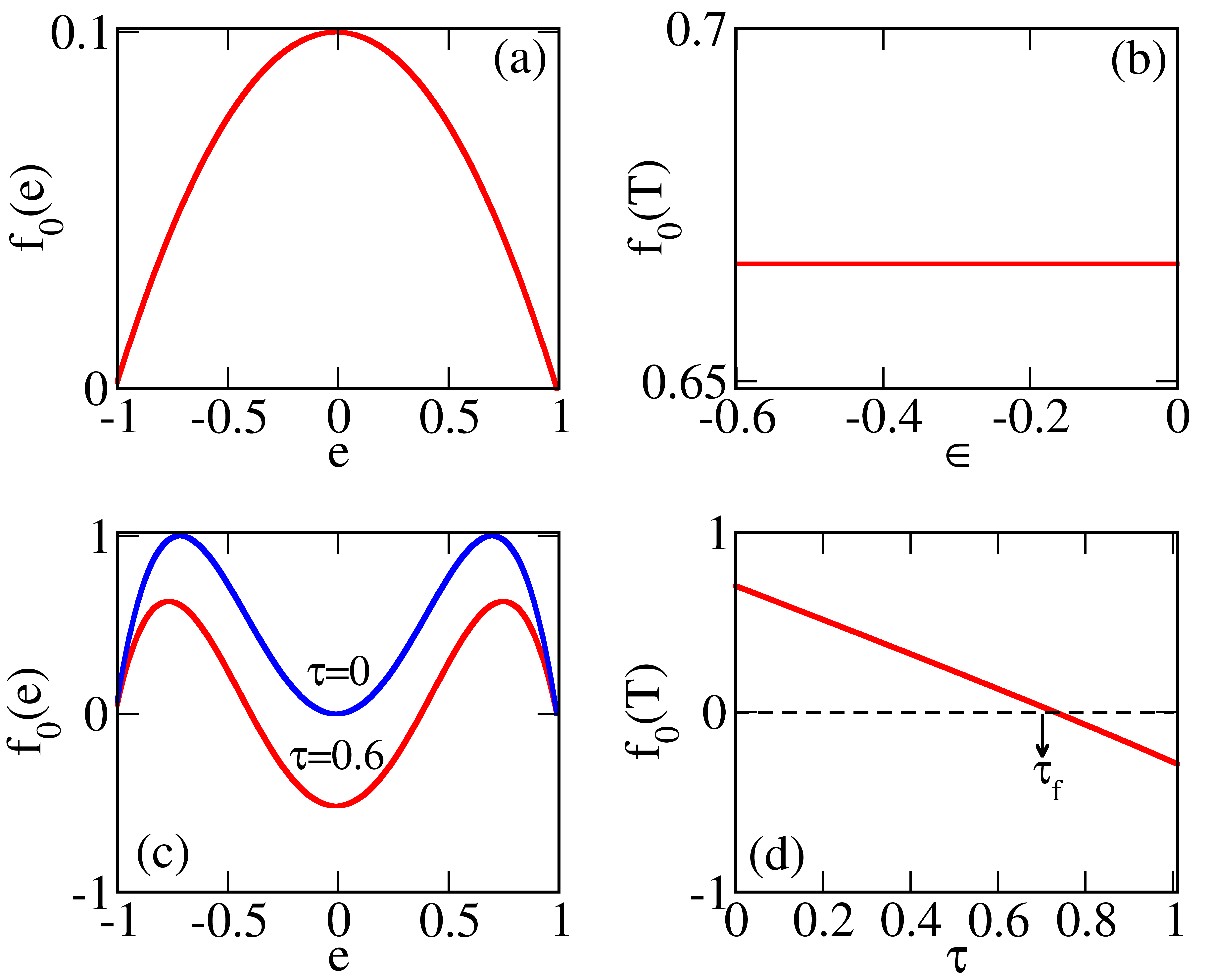
Figure 1: (Color online) BG case temperature dependent parameters: (a) Landau free energy density fLsubscript𝑓𝐿f_{L} vs order parameter e𝑒e, for various temperatures τ𝜏\tau. There are well-minima at ε¯¯𝜀\bar{\varepsilon}, and barrier-maxima at ε¯bsubscript¯𝜀𝑏{\bar{\varepsilon}}_{b}. (b) Mean-field order parameter ε¯¯𝜀\bar{\varepsilon} and barrier ε¯bsubscript¯𝜀𝑏{\bar{\varepsilon}}_{b}, vs τ𝜏\tau. (c) Scaling length ξscsubscript𝜉sc\xi_{\rm sc}, scaling time tscsubscript𝑡sct_{\rm sc}, and residual T𝑇T-dependence of ηsc(τ)subscript𝜂sc𝜏\eta_{\rm sc}(\tau), vs τ𝜏\tau.

Bales and Gooding (BG) have used a Lagrangian formalism to obtain R19 a continuous-strain, underdamped, momentum-conserving dynamics in 1D, for a one-component order parameter, or NOP=1subscript𝑁OP1N_{\rm OP}=1. For 1D, there is only one type of strain e=u(x)/x𝑒𝑢𝑥𝑥e=\partial u(x)/\partial x or gradient of displacement u(x)𝑢𝑥u(x), that is, the OP. The free energy F=E0xf𝐹subscript𝐸0subscript𝑥𝑓F=E_{0}\sum_{x}f where the free energy density f=fL+fG𝑓subscript𝑓𝐿subscript𝑓𝐺f=f_{L}+f_{G} is a sum of a triple-well Landau term fL=e62e4+τe2subscript𝑓𝐿superscript𝑒62superscript𝑒4𝜏superscript𝑒2f_{L}=e^{6}-2e^{4}+\tau e^{2}, and a Ginzburg term fGξ02(e/x)2similar-tosubscript𝑓𝐺superscriptsubscript𝜉02superscript𝑒𝑥2f_{G}\sim\xi_{0}^{2}(\partial e/\partial x)^{2}.

The Lagrangian density is ρ0e˙2fsubscript𝜌0superscript˙𝑒2𝑓\rho_{0}\dot{e}^{2}-f where in the “kinetic-energy” term, ρ0subscript𝜌0\rho_{0} is the mass of the unit cell of volume a0dsuperscriptsubscript𝑎0𝑑{a_{0}}^{d}, and the “potential-energy” is f𝑓f. With a Lagrangian minimization, and adding a Rayleigh dissipation term γe˙similar-toabsent𝛾˙𝑒\sim-\gamma\dot{e}, one gets R19

ρ0e¨(x,t)=(2x2)[Fe(x,t)γe˙(x,t)].(2.4)formulae-sequencesubscript𝜌0¨𝑒𝑥𝑡superscript2superscript𝑥2delimited-[]𝐹𝑒𝑥𝑡𝛾˙𝑒𝑥𝑡2.4\rho_{0}\ddot{e}(x,t)=\left(\frac{-\partial^{2}}{\partial x^{2}}\right)\left[\frac{-\partial F}{\partial e(x,t)}-\gamma\dot{e}(x,t)\right].~{}~{}(2.4)

Note that the long-wavelength k0𝑘0k\rightarrow 0 limit enforces global conservation of the total system momentum, with nonzero damping only for k0𝑘0\vec{k}\neq 0 internal momenta.

For higher spatial dimensions d=2𝑑2d=2 and 333, there are multiple strain components, describing the physical shear, compression and “deviatoric” or rectangular, distortions of the unit cell. A subset of the physical strains are the NOPsubscript𝑁OPN_{\rm OP} order parameter components that enter the nonlinear Landau free energy. The remaining non-OP physical strains are linked to the OP strains by R15 ; R16 “compatibility constraints” that ensure the distorted unit cells fit together in a smoothly compatible way, without dislocations. A constrained minimization yields an OP-OP effective interaction with an elastic constant prefactor A1subscript𝐴1A_{1}, that is, power-law and anisotropic, inducing preferred diagonal domain-wall orientations R15 ; R16 . We will throughout, set A1=0subscript𝐴10A_{1}=0, and consider these compatibility-induced interactions, elsewhere.

For a square-to-rectangle transition, the OP is the deviatoric strain written as e𝑒e, and as before, the free energy F=E0[fL+fG]𝐹subscript𝐸0delimited-[]subscript𝑓𝐿subscript𝑓𝐺F=E_{0}\sum[f_{L}+f_{G}]. The triple-well Landau term as shown in Fig 1(a), has minima at e=0𝑒0e=0, e=±ε¯(τ)𝑒plus-or-minus¯𝜀𝜏e=\pm{\bar{\varepsilon}}(\tau),

fL=[(τ1)e2+e2(e21)2],(2.5)subscript𝑓𝐿delimited-[]𝜏1superscript𝑒2superscript𝑒2superscriptsuperscript𝑒2122.5f_{L}=[(\tau-1)e^{2}+e^{2}(e^{2}-1)^{2}],~{}~{}(2.5)

with a scaled temperature defined as

τ(T)TTcT0Tc.(2.6a)formulae-sequence𝜏𝑇𝑇subscript𝑇𝑐subscript𝑇0subscript𝑇𝑐2.6𝑎\tau(T)\equiv\frac{T-T_{c}}{T_{0}-T_{c}}.~{}~{}(2.6a)

The minima are at e=±ε¯(τ)𝑒plus-or-minus¯𝜀𝜏e=\pm{\bar{\varepsilon}}(\tau), where

ε¯223[1+13τ/4],(2.6b)superscript¯𝜀223delimited-[]113𝜏42.6𝑏{\bar{\varepsilon}}^{2}\equiv\frac{2}{3}[1+\sqrt{1-3\tau/4}],~{}~{}(2.6b)

while the barriers between the austenite and martensite wells are at ε¯b(τ)223[113τ/4]subscript¯𝜀𝑏superscript𝜏223delimited-[]113𝜏4{\bar{\varepsilon}}_{b}(\tau)^{2}\equiv\frac{2}{3}[1-\sqrt{1-3\tau/4}]. Here, just below T=T0𝑇subscript𝑇0T=T_{0}, or τ(T0)=1𝜏subscript𝑇01\tau(T_{0})=1, when the triple wells are degenerate, the OP jumps from zero to unity ε¯(1)=1¯𝜀11\bar{\varepsilon}(1)=1. Below the austenite spinodal T=Tc𝑇subscript𝑇𝑐T=T_{c} or τ(Tc)=0𝜏subscript𝑇𝑐0\tau(T_{c})=0, the barriers vanish, ε¯b(τ=0)=0subscript¯𝜀𝑏𝜏00{\bar{\varepsilon}}_{b}(\tau=0)=0, and the metastable austenite minimum at e=0𝑒0e=0 disappears, (when the martensite minima are at ε¯(0)=±4/3¯𝜀0plus-or-minus43\bar{\varepsilon}(0)=\pm\sqrt{4/3}). At zero temperature, τ(0)=Tc/(T0Tc)𝜏0subscript𝑇𝑐subscript𝑇0subscript𝑇𝑐\tau(0)=-T_{c}/(T_{0}-T_{c}) (see Fig 1).

The Ginzburg term is

FG=E0ξ02(e)2,(2.7)subscript𝐹𝐺subscript𝐸0subscriptsuperscript𝜉20superscript𝑒22.7F_{G}=E_{0}\sum\xi^{2}_{0}(\vec{\nabla}e)^{2},~{}~{}(2.7)

where ξ0subscript𝜉0\xi_{0} is an OP bending length scale.

The underdamped dynamics is R20 ,

ρ0e¨(r,t)=c022[Fe+γe˙],(2.8)subscript𝜌0¨𝑒𝑟𝑡superscriptsubscript𝑐02superscript2delimited-[]𝐹𝑒𝛾˙𝑒2.8\rho_{0}\ddot{e}(\vec{r},t)=c_{0}^{2}\vec{\nabla}^{2}\left[\frac{\partial F}{\partial e}+\gamma\dot{e}\right],~{}~{}(2.8)

where c0=12subscript𝑐012c_{0}=\frac{1}{2} is a normalization. Here with a compatibility term fCA1=0similar-tosubscript𝑓𝐶subscript𝐴10f_{C}\sim A_{1}=0 suppressed, f=fL+fG𝑓subscript𝑓𝐿subscript𝑓𝐺f=f_{L}+f_{G}, and

fe(r,t)=fLe2ξ022e.(2.9)formulae-sequence𝑓𝑒𝑟𝑡subscript𝑓𝐿𝑒2superscriptsubscript𝜉02superscript2𝑒2.9\frac{\partial f}{\partial e({\vec{r}},t)}=\frac{\partial f_{L}}{\partial e}-2\xi_{0}^{2}{\vec{\nabla}}^{2}e.~{}~{}(2.9)

Re-defining space and time variables as before, ra0r;t(γ/2E0)tformulae-sequence𝑟subscript𝑎0𝑟𝑡𝛾2subscript𝐸0𝑡r\rightarrow a_{0}r;~{}~{}~{}t\rightarrow(\gamma/2E_{0})t, (2.8) becomes

Λ2e(r,t)t2=r2[μ(r,t)+e(r,t)t],(2.10)Λsuperscript2𝑒𝑟𝑡superscript𝑡2superscriptsubscript𝑟2delimited-[]𝜇𝑟𝑡𝑒𝑟𝑡𝑡2.10\Lambda\frac{\partial^{2}e(\vec{r},t)}{\partial t^{2}}={{\vec{\nabla}}_{\vec{r}}}^{2}\left[\mu(\vec{r},t)+\frac{\partial e(\vec{r},t)}{\partial t}\right],~{}~{}(2.10)

where the dimensionless Λγ2similar-toΛsuperscript𝛾2\Lambda\sim\gamma^{-2} is an inverse-damping squared and, with the unit-cell length a0=1subscript𝑎01a_{0}=1, is

Λ[2E0ρ0c02]1γ2.(2.11)formulae-sequenceΛdelimited-[]2subscript𝐸0subscript𝜌0superscriptsubscript𝑐021superscript𝛾22.11\Lambda\equiv\left[\frac{2E_{0}\rho_{0}}{c_{0}^{2}}\right]\frac{1}{\gamma^{2}}.~{}~{}~{}(2.11)

The chemical potential is

μ(r,t)=μLξ02r2e(r,t),(2.12)𝜇𝑟𝑡subscript𝜇𝐿superscriptsubscript𝜉02superscriptsubscript𝑟2𝑒𝑟𝑡2.12\mu(\vec{r},t)=\mu_{L}-{\xi_{0}}^{2}{\vec{\nabla}}_{\vec{r}}^{2}e(\vec{r},t),~{}~{}(2.12)

where μL(1/2)fL/e=e[τ4e2+3e4]subscript𝜇𝐿12subscript𝑓𝐿𝑒𝑒delimited-[]𝜏4superscript𝑒23superscript𝑒4\mu_{L}\equiv(1/2)\partial f_{L}/\partial e=e[\tau-4e^{2}+3e^{4}].

II.3 Scaling out the OP T𝑇T-dependence

As is well-known R1 ; R2 ; R4 , the CH dynamics can be cast in T𝑇T-independent form, by scaling the OP by its Landau-minimum value, and introducing T𝑇T-dependent length and time scales, as

eε¯e;rrξsc(T);tttsc(T),(2.13)formulae-sequence𝑒¯𝜀𝑒formulae-sequence𝑟𝑟subscript𝜉sc𝑇𝑡𝑡subscript𝑡sc𝑇2.13e\rightarrow{\bar{\varepsilon}}~{}e~{};r\rightarrow r~{}\xi_{\rm sc}(T);~{}t\rightarrow t~{}t_{\rm sc}(T),~{}~{}(2.13)

where ε¯=|ϵ|1/2¯𝜀superscriptitalic-ϵ12{\bar{\varepsilon}}=|\epsilon|^{1/2}. The kinetic term on the left side of (2.3) then has a factor ξsc4/tscsuperscriptsubscript𝜉sc4subscript𝑡sc\xi_{\rm sc}^{4}/t_{\rm sc}, while the Landau term on right side has a factor ξsc2ε¯2superscriptsubscript𝜉sc2superscript¯𝜀2\xi_{\rm sc}^{2}{\bar{\varepsilon}}^{2}. Setting both equal to unity, the scaling length is seen to be the Ginzburg-Landau correlation length ξsc=1/ε¯=1/|ϵ|1/2=ξGL(T)subscript𝜉sc1¯𝜀1superscriptitalic-ϵ12subscript𝜉𝐺𝐿𝑇\xi_{\rm sc}=1/{\bar{\varepsilon}}=1/|\epsilon|^{1/2}=\xi_{GL}(T), while the scaling time is tsc=1/ε¯4=1/|ϵ|2subscript𝑡sc1superscript¯𝜀41superscriptitalic-ϵ2t_{\rm sc}=1/{\bar{\varepsilon}}^{4}=1/|\epsilon|^{2}. The OP-scaled CH dynamics is then in the T𝑇T-independent form,

e/t=2μLξ024e,(2.14)𝑒𝑡superscript2subscript𝜇𝐿superscriptsubscript𝜉02superscript4𝑒2.14\partial e/\partial t={\vec{\nabla}^{2}}\mu_{L}-\xi_{0}^{2}{\vec{\nabla}^{4}}e,~{}~{}(2.14)

where μL=ef0(e)subscript𝜇𝐿𝑒subscript𝑓0𝑒\mu_{L}=-ef_{0}(e), with a scaled factor f0=(1e2)subscript𝑓01superscript𝑒2f_{0}=(1-e^{2}), that vanishes in the bulk.

For the BG case, the OP-scaling of (2.13) yields factors of the same type (ξsc2/tsc)2superscriptsuperscriptsubscript𝜉sc2subscript𝑡sc2(\xi_{\rm sc}^{2}/t_{\rm sc})^{2}, and ξsc2/tscsuperscriptsubscript𝜉sc2subscript𝑡sc\xi_{\rm sc}^{2}/t_{\rm sc}, for the inertial and damping terms, respectively, while the Landau term has a factor ξsc2ε¯4superscriptsubscript𝜉sc2superscript¯𝜀4\xi_{\rm sc}^{2}{\bar{\varepsilon}}^{4}. Setting these to unity, ξsc=1/ε¯2(τ),tsc=1/ε¯4(τ)formulae-sequencesubscript𝜉sc1superscript¯𝜀2𝜏subscript𝑡sc1superscript¯𝜀4𝜏\xi_{\rm sc}=1/{\bar{\varepsilon}}^{2}(\tau),~{}t_{\rm sc}=1/{\bar{\varepsilon}}^{4}(\tau). The OP-scaled BG dynamics without compatibility interactions is

Λ2e/t2=2[μL+e/t]ξ024e,(2.15)Λsuperscript2𝑒superscript𝑡2superscript2delimited-[]subscript𝜇𝐿𝑒𝑡superscriptsubscript𝜉02superscript4𝑒2.15\Lambda\partial^{2}e/\partial t^{2}={\vec{\nabla}^{2}}[\mu_{L}+\partial e/\partial t]-\xi_{0}^{2}{\vec{\nabla}^{4}}e,~{}~{}(2.15)

where μL=ef0(e)subscript𝜇𝐿𝑒subscript𝑓0𝑒\mu_{L}=-ef_{0}(e) with f0=3(1e2)(e2ηsc(T))subscript𝑓031superscript𝑒2superscript𝑒2subscript𝜂sc𝑇f_{0}=3(1-e^{2})(e^{2}-\eta_{\rm sc}(T)). Thus for a first-order transition, scaling the OP by its Landau value still leaves behind a residual temperature-dependence, through

ηsc(T)τ/3ε¯4,(2.16)subscript𝜂sc𝑇𝜏3superscript¯𝜀42.16\eta_{\rm sc}(T)\equiv\tau/3{\bar{\varepsilon}}^{4},~{}~{}(2.16)

that is negative for τ<0𝜏0\tau<0 below the spinodal, and for τ>0𝜏0\tau>0 is essentially the (positive) ratio of barrier height to well depth, ηsc=[ε¯b(τ)/ε¯(τ)]2subscript𝜂scsuperscriptdelimited-[]subscript¯𝜀𝑏𝜏¯𝜀𝜏2\eta_{\rm sc}=[{\bar{\varepsilon}}_{b}(\tau)/~{}{\bar{\varepsilon}}(\tau)]^{2} [see Fig 1(c)].

For the numerical simulations of Sec. IV, we will use the unscaled or T𝑇T-dependent forms (2.3), (2.10), and only later multiply the curvature-evolution data by the scaling lengths and times. For the theoretical analysis of Sec. V, we will use the “OP-scaled” forms (2.14), and (2.15).

III Strain correlations and dynamical scaling

In this section, we define the OP-OP and related correlations, and their dynamical scaling forms.

For a one-component martensitic-strain order parameter e(r,t)𝑒𝑟𝑡e(\vec{r},t), we consider a two-point correlation between OP’s at r=R+r0𝑟𝑅subscript𝑟0\vec{r}=\vec{R}+\vec{r}_{0}, and r=r0superscript𝑟subscript𝑟0\vec{r^{\prime}}=\vec{r}_{0} on a d𝑑d-dimensional lattice, and at equal times t𝑡t. With an average over all origins r0subscript𝑟0{\vec{r}_{0}} and over many runs, OP-OP correlations are dependent only on the separation R=rr𝑅𝑟superscript𝑟\vec{R}=\vec{r}-\vec{r^{\prime}},

C(R,t)=e(r,t)e(r,t),(3.1a)𝐶𝑅𝑡delimited-⟨⟩𝑒𝑟𝑡𝑒superscript𝑟𝑡3.1𝑎C(\vec{R},t)=\langle e(\vec{r},t)e(\vec{r^{\prime}},t)\rangle,~{}~{}(3.1a)
=1Nr0<e(R+r0,t)e(r0,t)>.(3.1b)formulae-sequenceabsent1𝑁subscriptsubscript𝑟0expectation𝑒𝑅subscript𝑟0𝑡𝑒subscript𝑟0𝑡3.1𝑏=\frac{1}{N}\sum_{r_{0}}<e({\vec{R}}+{\vec{r}}_{0},t)e({\vec{r}}_{0},t)>.~{}~{}(3.1b)

With a Fourier expansion e(r,t)=1Nkeikre(k,t)𝑒𝑟𝑡1𝑁subscript𝑘superscript𝑒𝑖𝑘𝑟𝑒𝑘𝑡e(\vec{r},t)=\frac{1}{\sqrt{N}}\sum_{\vec{k}}e^{i\vec{k}\cdot\vec{r}}e(\vec{k},t), we get

C(R,t)=kS(k,t)eikR,(3.2a)𝐶𝑅𝑡subscript𝑘𝑆𝑘𝑡superscript𝑒𝑖𝑘𝑅3.2𝑎C(\vec{R},t)=\sum_{\vec{k}}S(\vec{k},t)e^{i\vec{k}\cdot\vec{R}},~{}~{}(3.2a)

where the time-dependent structure factor is

S(k,t)=|e(k,t)|2.(3.2b)formulae-sequence𝑆𝑘𝑡delimited-⟨⟩superscript𝑒𝑘𝑡23.2𝑏S(\vec{k},t)=\langle|e(k,t)|^{2}\rangle.~{}~{}(3.2b)

Since the OP is real, its Fourier coefficients e(k,t)=e(k,t)𝑒superscript𝑘𝑡𝑒𝑘𝑡e(\vec{k},t)^{*}=e(-\vec{k},t) and so S(k,t)=S(k,t)𝑆𝑘𝑡𝑆𝑘𝑡S(\vec{k},t)=S(-\vec{k},t).

Another correlation that enters is the chemical potential-order parameter or μ𝜇\mu-OP correlation:

C(μ)(R,t)=μ(r,t)e(r,t)(3.3a)superscript𝐶𝜇𝑅𝑡delimited-⟨⟩𝜇𝑟𝑡𝑒superscript𝑟𝑡3.3𝑎C^{(\mu)}(\vec{R},t)=\langle\mu(\vec{r},t)e(\vec{r^{\prime}},t)\rangle~{}~{}(3.3a)
=1Nr0μ(R+r0,t)e(r0,t).(3.3b)formulae-sequenceabsentdelimited-⟨⟩1𝑁subscriptsubscript𝑟0𝜇𝑅subscript𝑟0𝑡𝑒subscript𝑟0𝑡3.3𝑏=\left\langle\frac{1}{N}\sum_{r_{0}}\mu({\vec{R}}+{\vec{r}}_{0},t)e({\vec{r}}_{0},t)\right\rangle.~{}~{}~{}(3.3b)

With a Fourier expansion μ(r,t)=1Nkeikrμ(k,t)𝜇𝑟𝑡1𝑁subscript𝑘superscript𝑒𝑖𝑘𝑟𝜇𝑘𝑡\mu(\vec{r},t)=\frac{1}{\sqrt{N}}\sum_{\vec{k}}e^{i\vec{k}\cdot\vec{r}}\mu(\vec{k},t), we get

C(μ)(R,t)=kS(μ)(k,t)eikR,(3.4a)superscript𝐶𝜇𝑅𝑡subscript𝑘superscript𝑆𝜇𝑘𝑡superscript𝑒𝑖𝑘𝑅3.4𝑎C^{(\mu)}(\vec{R},t)=\sum_{\vec{k}}S^{(\mu)}(\vec{k},t)e^{i\vec{k}\cdot\vec{R}},~{}~{}~{}~{}(3.4a)

where only the symmetric part survives, and the μ𝜇\mu-OP Fourier correlation is the real part,

S(μ)(k,t)=Reμ(k,t)e(k,t).(3.4b)formulae-sequencesuperscript𝑆𝜇𝑘𝑡𝑅𝑒delimited-⟨⟩𝜇𝑘𝑡𝑒superscript𝑘𝑡3.4𝑏S^{(\mu)}(\vec{k},t)=Re\langle\mu(\vec{k},t)e(\vec{k},t)^{\ast}\rangle.~{}~{}(3.4b)

Since the anisotropic compatibility interaction is switched off, the system is isotropic, and we can work throughout with averages <>expectation<...> that now include angular averages, so correlations become C(R,t)C(R,t)𝐶𝑅𝑡𝐶𝑅𝑡C(\vec{R},t)\rightarrow C(R,t) and S(k,t)S(k,t)𝑆𝑘𝑡𝑆𝑘𝑡S(\vec{k},t)\rightarrow S(k,t),S(μ)(k,t)S(μ)(k,t)superscript𝑆𝜇𝑘𝑡superscript𝑆𝜇𝑘𝑡S^{(\mu)}(\vec{k},t)\rightarrow S^{(\mu)}(k,t) where R|R|𝑅𝑅R\equiv|\vec{R}|, and k|k|𝑘𝑘k\equiv|\vec{k}|.

The OP-OP correlation C(R,t)𝐶𝑅𝑡C(R,t) for a given time t𝑡t will show a fall-off in separation R𝑅R; while at a given separation R𝑅R, it will increase with time. Since L(t)similar-toabsent𝐿𝑡\sim L(t) is the scale of the OP-correlation region, it will also increase with t𝑡t. As L(t)𝐿𝑡L(t) is also the separation of the OP-dips at domain walls, these strain patterns must coarsen with time.

Dynamical scaling says that R1 ; R13 (i) the time t𝑡t enters only through the length L(t)𝐿𝑡L(t); (ii) the separation R𝑅R appears only in scaled form as R¯R/L(t)¯𝑅𝑅𝐿𝑡\bar{R}\equiv R/L(t), [and in Fourier space, the wave vector k𝑘k appears only as k¯kL(t)¯𝑘𝑘𝐿𝑡\bar{k}\equiv kL(t)]. Further, in a common assumption, (iii) the coarsening length scale grows as a power law Ltαsimilar-to𝐿superscript𝑡𝛼L\sim t^{\alpha}, which is plausible R1 , but here is justified. The OP-OP correlation is then

C(R,t)/C(0,t)=G(R/L(t))G(R¯).(3.5)formulae-sequence𝐶𝑅𝑡𝐶0𝑡𝐺𝑅𝐿𝑡𝐺¯𝑅3.5C(R,t)/C(0,t)=G(R/L(t))\equiv G(\bar{R}).~{}~{}~{}(3.5)

We find later that the zero-separation values, in a few hundred time steps, on the onset of dynamical scaling, are insensitive to time, C(0,t)C(0,tonset)similar-to-or-equals𝐶0𝑡𝐶0subscript𝑡onsetC(0,t)\simeq C(0,t_{\rm onset}), so we henceforth suppress the constant denominator.

In Fourier space, the scaling behaviour is

S(k,t)=Ldχ(kL(t))Ldχ(k¯).(3.6)formulae-sequence𝑆𝑘𝑡superscript𝐿𝑑𝜒𝑘𝐿𝑡superscript𝐿𝑑𝜒¯𝑘3.6S(k,t)=L^{d}\chi(kL(t))\equiv L^{d}\chi(\bar{k}).~{}~{}~{}(3.6)

For sharp domain walls, of widths small compared to L(t)𝐿𝑡L(t), Porod’s law holds for the Fourier space structure factor R1 ; R7

χ(k¯)1/[k¯]d+NOP.(3.7)formulae-sequencesimilar-to-or-equals𝜒¯𝑘1superscriptdelimited-[]¯𝑘𝑑subscript𝑁OP3.7\chi(\bar{k})\simeq 1/[\bar{k}]^{d+N_{\rm OP}}.~{}~{}~{}(3.7)

For NOP=1subscript𝑁OP1N_{\rm OP}=1, we have χ1/(kL)d+1similar-to-or-equals𝜒1superscript𝑘𝐿𝑑1\chi\simeq 1/(kL)^{d+1}, and a log-log plot of S(k,t)𝑆𝑘𝑡S(k,t) versus k𝑘k will be a straight line with slope (d+1)𝑑1-(d+1), with the length L(t)𝐿𝑡L(t) extracted from the intercepts lnχ=(d+1)lnklnL(t)𝜒𝑑1𝑘𝐿𝑡\ln\chi=-(d+1)\ln k-\ln L(t). Then with this scaling length, replots of lnχ𝜒\ln\chi versus ln(k¯)¯𝑘\ln(\bar{k}), as well as G(R¯)𝐺¯𝑅G(\bar{R}) versus R¯¯𝑅\bar{R}, will show data collapse of different-time curves.

The coarsening curvature is defined R1 as (d1)/L(t)𝑑1𝐿𝑡(d-1)/L(t), but we will simply work with an inverse length, or

g(t)1/L(t),(3.8)𝑔𝑡1𝐿𝑡3.8g(t)\equiv 1/L(t),~{}~{}~{}(3.8)

and call this the “curvature,” as it indeed is, for d=2𝑑2d=2. Thus the scaled variables are

R¯g(t)R;k¯k/g(t).(3.9)formulae-sequenceformulae-sequence¯𝑅𝑔𝑡𝑅¯𝑘𝑘𝑔𝑡3.9\bar{R}\equiv g(t)R~{};\bar{k}\equiv k/g(t).~{}~{}~{}(3.9)

We later show that the correlation dynamics results in a nonlinear kinetics for the curvature g(t)𝑔𝑡g(t), that has power-law solutions g1/tαsimilar-to𝑔1superscript𝑡𝛼g\sim 1/t^{\alpha}, explaining the observed coarsening-length behaviour Ltαsimilar-to𝐿superscript𝑡𝛼L\sim t^{\alpha}.

IV Numerical results on dynamical scaling

In this section, we present numerical work, showing domain-wall (DW) textures, demonstrating dynamical scaling, and extracting exponent behaviour of coarsening curvatures. In an actual experimental quench, the physical temperature is changed suddenly, and the coarsening probe is followed in physical time. Any universal curve independent of quench temperatures T𝑇T, is obtained only by later scaling the measured physical values, by factors dependent on T𝑇T. As mentioned, we mimic this experimental procedure in simulations by using the unscaled forms of both the CH and BG dynamics in (2.3)and (2.10); only then doing scaling on the numerical data obtained.
Refer to caption
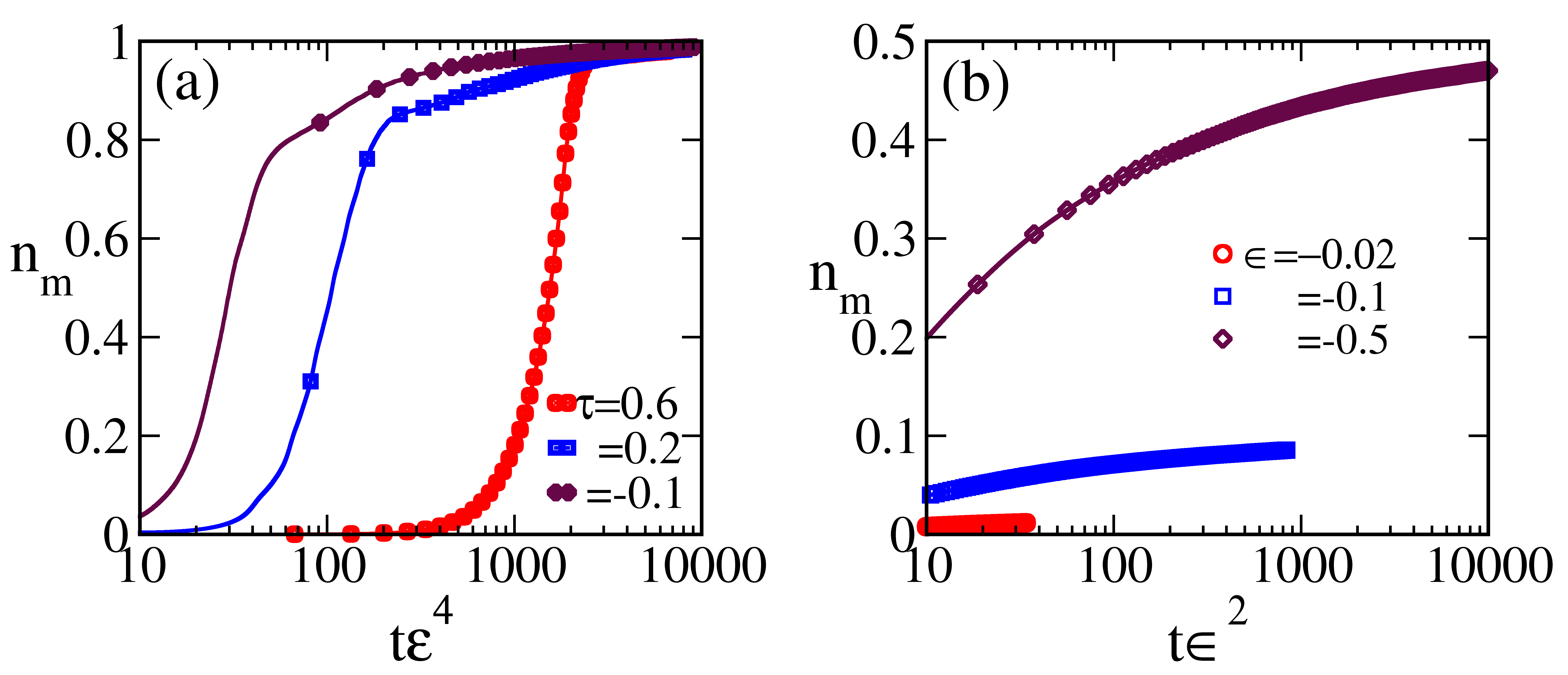
Figure 2: (Color online) Ordered-fraction evolutions: (a) BG case martensitic-ordered fraction nmsubscript𝑛𝑚n_{m} versus scaled time tε¯(τ)4𝑡¯𝜀superscript𝜏4t{\bar{\varepsilon}}(\tau)^{4}, for quenches τ=0.1,0.2,0.6𝜏0.10.20.6\tau=-0.1,0.2,0.6. (b) CH case ordered fraction nmsubscript𝑛𝑚n_{m} versus scaled time tε¯4=tϵ(T)2𝑡superscript¯𝜀4𝑡italic-ϵsuperscript𝑇2t{\bar{\varepsilon}}^{4}=t~{}\epsilon(T)^{2}, for quenches to ϵ(T/Tc1)=0.5,0.1,0.02formulae-sequenceitalic-ϵ𝑇subscript𝑇𝑐10.50.10.02\epsilon\equiv(T/T_{c}-1)=-0.5,-0.1,-0.02. Critical slowing down is seen close to Tcsubscript𝑇𝑐T_{c}, with ordered-fractions rising only slowly, within the holding-time t<th𝑡subscript𝑡t<t_{h}.

The initial high-temperature state for both the CH and BG cases, corresponds to a single well, with a minimum at e(r,t=0)=0𝑒𝑟𝑡00e(\vec{r},t=0)=0, plus a few local fluctuations of the ordered variants. A numerical “quench” then corresponds to evolving at some suddenly lower temperature T𝑇T. There will be an early-time regime where the ordered phases expand, to crowd out the initially dominant e=0𝑒0e=0 background as a DW vapour phase; while at intermediate and long times, there will be only competing variants, separated by domain walls, as a DW liquid phase.
Refer to caption
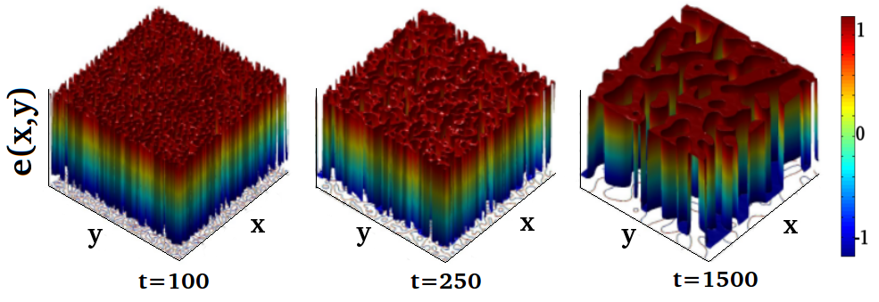
Figure 3: (Color online) Relief plot of coarsening: Snapshots for various times, showing coarsening of the OP strain e(r,t)𝑒𝑟𝑡e({\vec{r}},t) after a quench, for system size 5122superscript5122512^{2}.Positive/negative/zero strains are red/blue/green. See cross-sectional slices.The top of the relief plot shows positive (red) regions, plunging down through valleys, to reach complementary negative (blue) values, passing through domain walls regions, where order parameters go through zero (green).

We thus start with a dilute set of initial seeds of both martensite variants equally, in a sea of e=0𝑒0e=0 austenite. The martensite conversion fraction nm(t)1Nre2(r,t)/|ε¯|subscript𝑛𝑚𝑡1𝑁subscript𝑟superscript𝑒2𝑟𝑡¯𝜀n_{m}(t)\equiv\frac{1}{N}\sum_{\vec{r}}e^{2}(\vec{r},t)/|\bar{\varepsilon}| is initially nonzero only at 2%percent22\% random sites surrounded by 2×2222\times 2 unit cells where e=±ε¯𝑒plus-or-minus¯𝜀e=\pm{\bar{\varepsilon}}, with e=0𝑒0e=0 elsewhere, and so nm(0)=0.08subscript𝑛𝑚00.08n_{m}(0)=0.08.

Refer to caption
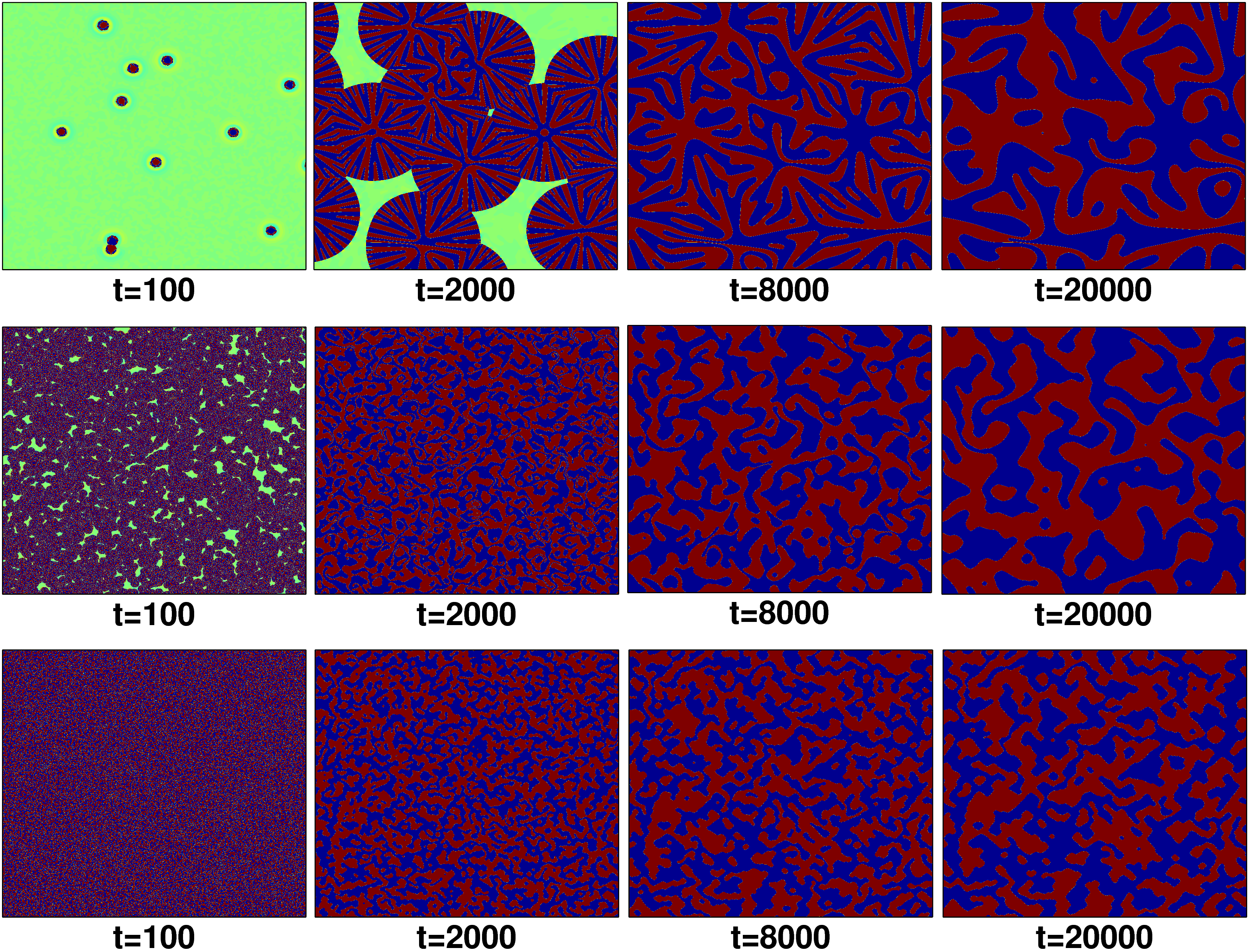
Figure 4: (Color online) Contour-plots of strain evolutions: Snapshots of e(r,t)𝑒𝑟𝑡e(\vec{r},t) textures, held at fixed quench temperatures, up to a holding time th=20,000subscript𝑡20000t_{h}=20,000 for system size 81922superscript819228192^{2}; the pictures are zoomed in to an area of 40962superscript409624096^{2}. (a) First row: shallow quench to τ=0.6𝜏0.6\tau=0.6, or Δτ=0.1Δ𝜏0.1\Delta\tau=-0.1; (b) Second row: moderate quench to τ=0.2𝜏0.2\tau=0.2, or Δτ=0.5Δ𝜏0.5\Delta\tau=-0.5; (c) Third row: deep quench to τ=0.1𝜏0.1\tau=-0.1, or Δτ=0.8Δ𝜏0.8\Delta\tau=-0.8, when coarsening seems to slow, suggesting a glassy state.

We use an Euler-discretized dynamics of (2.3), (2.10) to find the OP evolution of e(r,t)𝑒𝑟𝑡e(\vec{r},t), focusing on Λ=1Λ1\Lambda=1. We take time steps Δt=0.05Δ𝑡0.05\Delta t=0.05; and spatial derivatives νsubscript𝜈\nabla_{\nu} as finite-difference operators (a0)1Δνsuperscriptsubscript𝑎01subscriptΔ𝜈(a_{0})^{-1}\Delta_{\nu} on a square unit lattice. For wave vectors k𝑘\vec{k} in the Brillouin zone, Δν2sin(kνa0/2)subscriptΔ𝜈2subscript𝑘𝜈subscript𝑎02\Delta_{\nu}\rightarrow 2\sin(k_{\nu}a_{0}/2) , with the grid scale set to a0=1subscript𝑎01a_{0}=1. A fast Fourier transform yields the Fourier coefficient e(k,t)𝑒𝑘𝑡e(\vec{k},t); and hence the angularly averaged dynamic structure factor S(k,t)=<|e(k,t)|2>𝑆𝑘𝑡expectationsuperscript𝑒𝑘𝑡2S(k,t)=<|e(\vec{k},t)|^{2}> of (3.2). (To focus on DW time scales, a “strain-hardening” procedure is used R9 .) Run averages are taken, over Nrun=5subscript𝑁𝑟𝑢𝑛5N_{run}=5. A reverse FFT yields the OP-OP correlations C(R,t)𝐶𝑅𝑡C(R,t) of (3.1). The quench temperature T𝑇T is held fixed, for a holding time th=20,000subscript𝑡20000t_{h}=20,000 steps. The 2D system is of size Lsys2=81922superscriptsubscript𝐿sys2superscript81922L_{\rm sys}^{2}=8192^{2}.

Figure 2(a) shows the BG case single-run martensite or ordered-fraction nm(t)subscript𝑛𝑚𝑡n_{m}(t) versus scaled time tε¯4(τ)𝑡superscript¯𝜀4𝜏t\bar{\varepsilon}^{4}(\tau). For temperatures just below T=T4𝑇subscript𝑇4T=T_{4} or τ=τ(T4)=0.74𝜏𝜏subscript𝑇40.74\tau=\tau(T_{4})=0.74 the martensite fraction rises slowly towards unity, with larger delays, closer to T4subscript𝑇4T_{4}. Above T4subscript𝑇4T_{4} there is no conversion at all, as the initial martensite seeds dissolve back into the four-fold symmetry austenite. We will quench to temperatures sufficiently below T4subscript𝑇4T_{4} so conversion delays are small.

Refer to caption
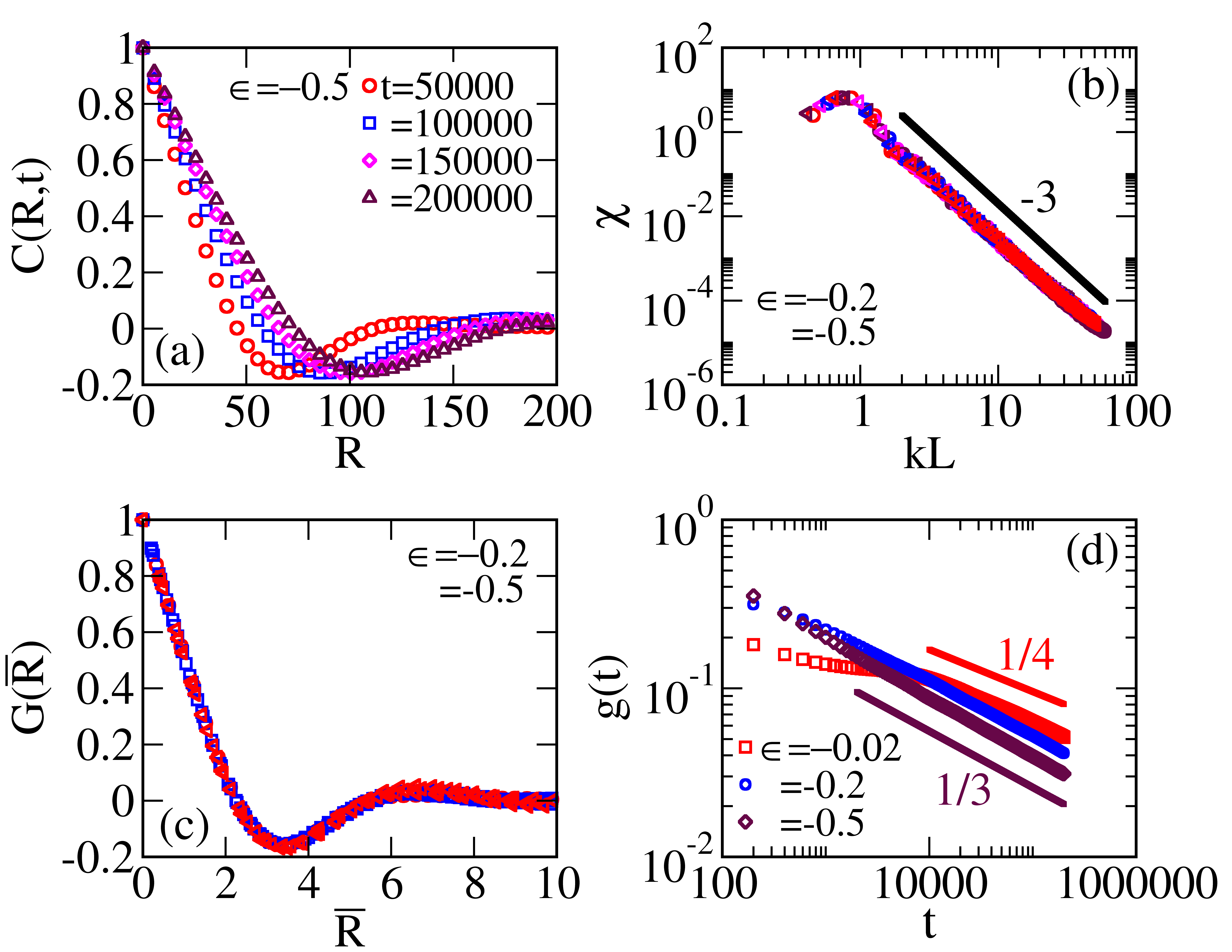
Figure 5: (Color online) Cahn-Hilliard OP correlations for various quenches : (a) For ϵ=0.5italic-ϵ0.5\epsilon=-0.5, data for C(R,t)𝐶𝑅𝑡C(R,t) vs R𝑅R for various times t𝑡t; (b) Porod’s Law behaviour in scaled structure factor χ(kL)𝜒𝑘𝐿\chi(kL) vs scaled wave-vector kL(t)𝑘𝐿𝑡kL(t), showing data collapse in Fourier space, for all times and temperatures; (c) Dynamical scaling in G(R¯)𝐺¯𝑅G(\bar{R}) vs scaled separation R¯R/L¯𝑅𝑅𝐿\bar{R}\equiv R/L, showing data collapse in coordinate space, for all times, and temperatures; (d) Log-log plot of unscaled curvature g(t)1/L(t)𝑔𝑡1𝐿𝑡g(t)\equiv 1/L(t) vs time t𝑡t, showing “guide to the eye” indicated exponents α=1/4,1/3𝛼1413\alpha=1/4,1/3, seen within the holding time thsubscript𝑡t_{h}.
Refer to caption
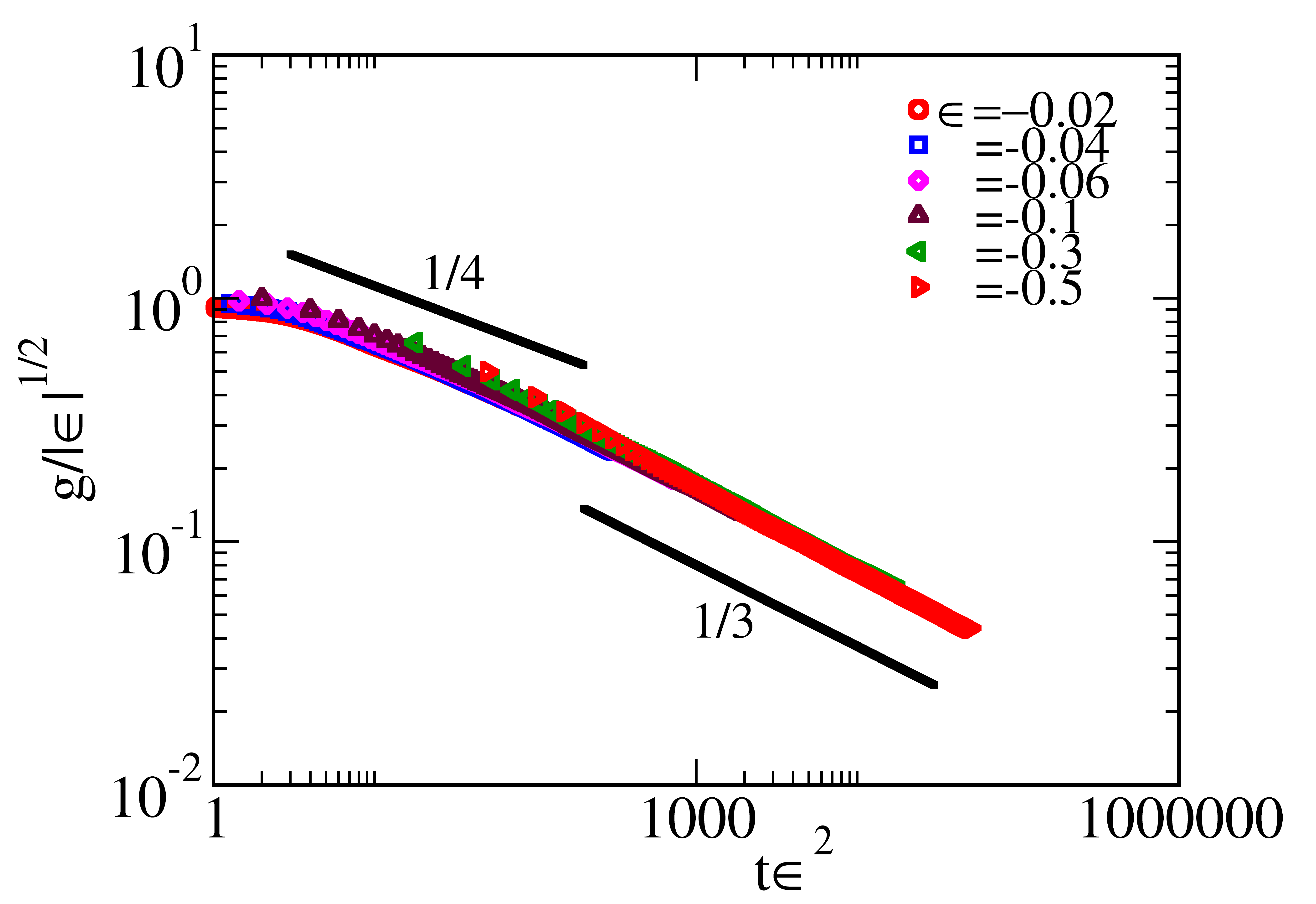
Figure 6: (Color online) CH curvature coarsening and scaled variables: Plot of previous CH data of Fig. 5(d), in scaled variables, showing g/ε¯=g/|ϵ|1/2𝑔¯𝜀𝑔superscriptitalic-ϵ12g/{\bar{\varepsilon}}=g/|\epsilon|^{1/2} vs tε¯4=t|ϵ|2𝑡superscript¯𝜀4𝑡superscriptitalic-ϵ2t~{}{\bar{\varepsilon}}^{4}=t~{}|\epsilon|^{2}. There is data collapse for all temperatures, and guide to the eye lines indicate exponents of α=1/4𝛼14\alpha=1/4 for intermediate times, crossing over to α=1/3𝛼13\alpha=1/3 for long times.
Refer to caption
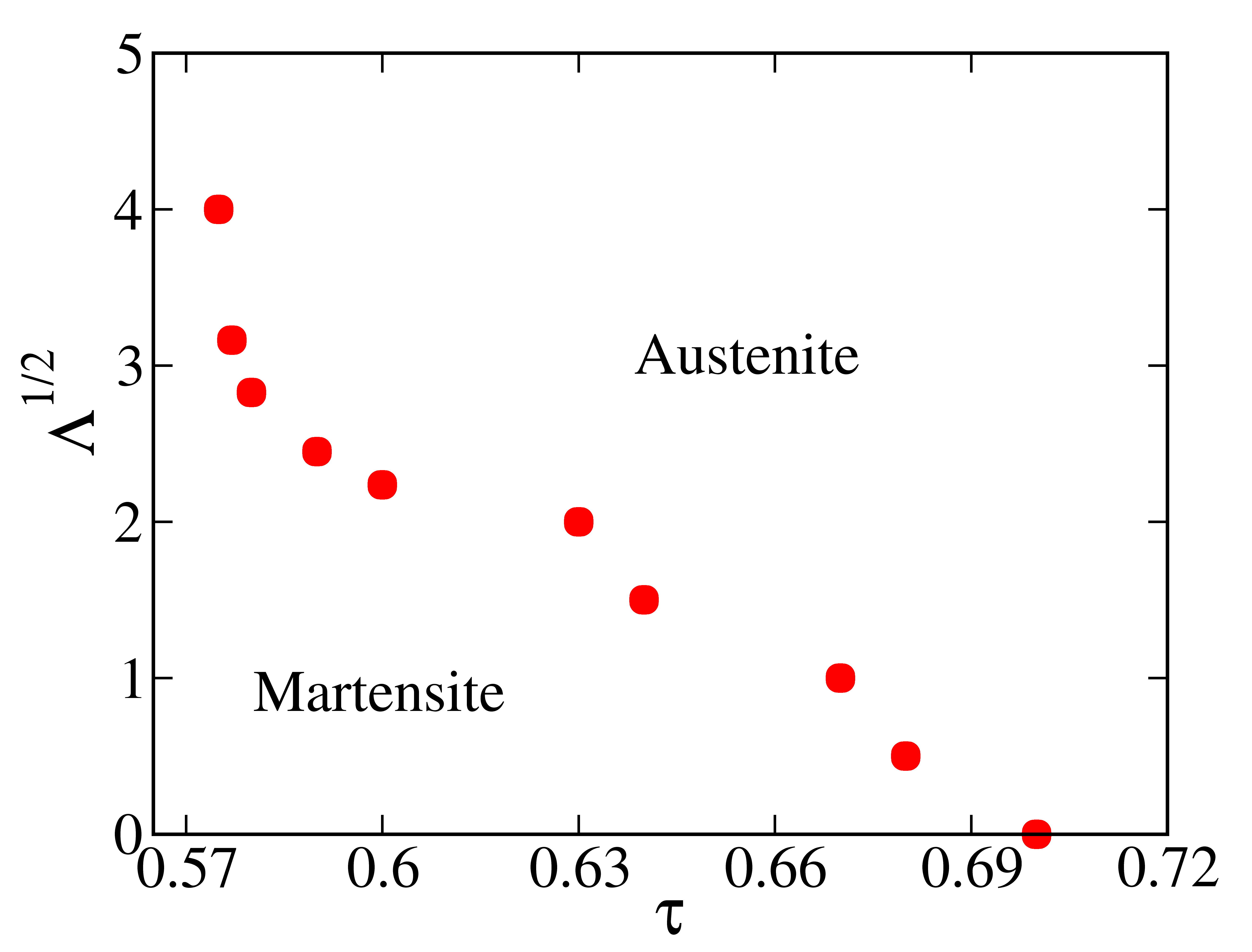
Figure 7: (Color online) Phase diagram: Inverse damping ΛΛ\Lambda versus scaled quench temperature τ𝜏\tau, with austenite above the transition-temperature curve, and martensite, below it.
Refer to caption
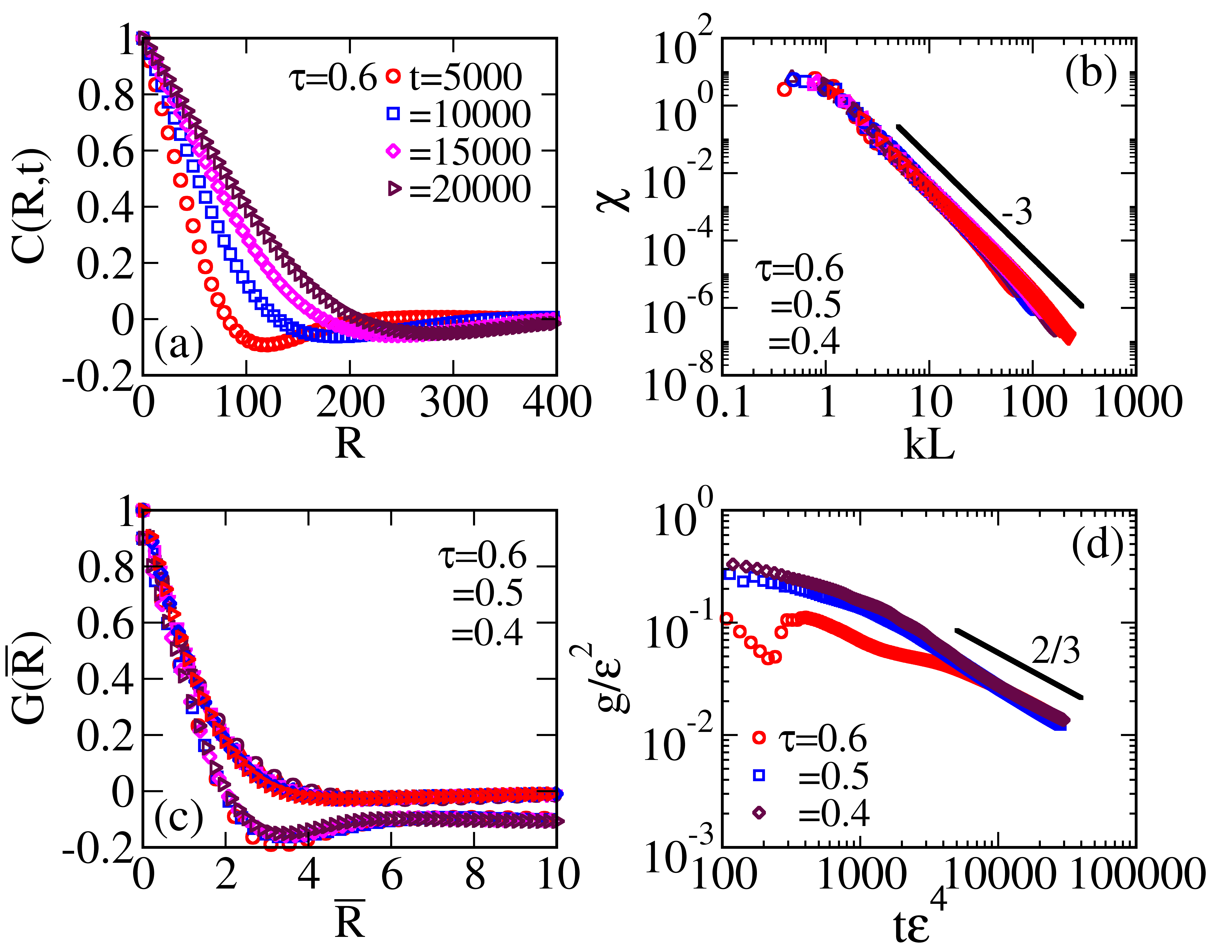
Figure 8: (Color online) Bales-Gooding OP correlations for shallow quenches: (a) For τ=0.6𝜏0.6\tau=0.6, data for C(R,t)𝐶𝑅𝑡C(R,t) versus R𝑅R for various times; (b) Porod’s Law behaviour in scaled structure factor χ(kL)𝜒𝑘𝐿\chi(kL) versus scaled wave-vector kL(t)𝑘𝐿𝑡kL(t) showing data collapse in Fourier space, for all times ; (c) Dynamical scaling in G(R¯)𝐺¯𝑅G(\bar{R}) versus scaled separation R¯R/L¯𝑅𝑅𝐿\bar{R}\equiv R/L showing data collapse in coordinate space, for all times. The scaled curves actually have slightly different shapes, for different temperatures, due to residual τ𝜏\tau dependence, and the τ=0.6𝜏0.6\tau=0.6 curve is shifted downwards by 0.10.10.1, to highlight this.For decreasing temperatures τ=0.5,0.4𝜏0.50.4\tau=0.5,0.4 the curves are closer in shape and values, so the data are not relatively shifted. (d) Log-Log plot of scaled coarsening curvature g(t)/ε¯(τ)2𝑔𝑡¯𝜀superscript𝜏2g(t)/{\bar{\varepsilon}}(\tau)^{2}, vs tε¯(τ)4𝑡¯𝜀superscript𝜏4t~{}{\bar{\varepsilon}}(\tau)^{4}, with indicated exponents α=2/3𝛼23\alpha=2/3 seen, within thsubscript𝑡t_{h}.
Refer to caption
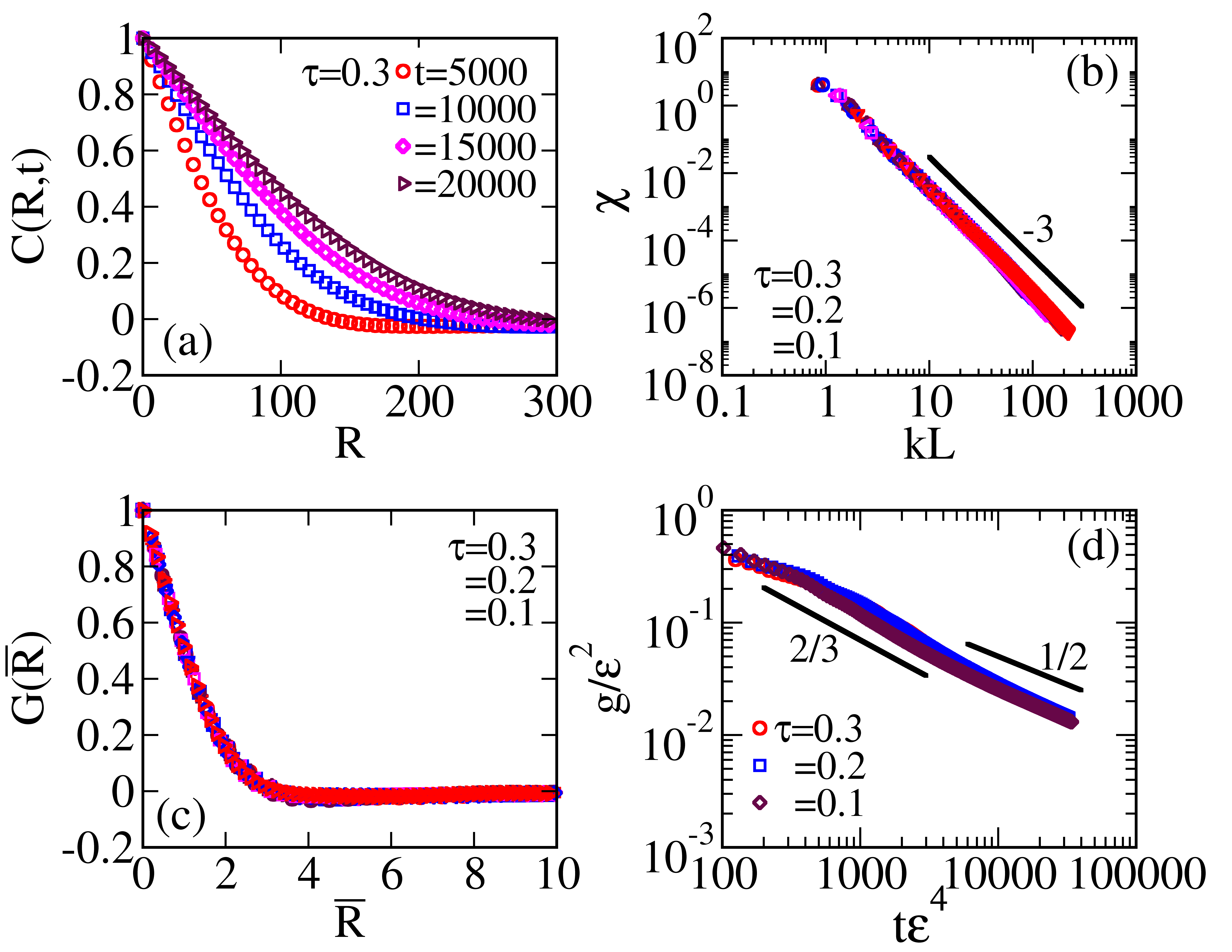
Figure 9: (Color online) Bales-Gooding OP correlations for moderate quenches: (a) For τ=0.3𝜏0.3\tau=0.3, data for C(R,t)𝐶𝑅𝑡C(R,t) versus R𝑅R for various times; (b) Porod’s Law behaviour in scaled structure factor χ(kL)𝜒𝑘𝐿\chi(kL) versus scaled wave-vector kL(t)𝑘𝐿𝑡kL(t), showing data collapse in Fourier space for all times; (c) Dynamical scaling in G(R¯)𝐺¯𝑅G(\bar{R}) versus scaled separation R¯R/L¯𝑅𝑅𝐿\bar{R}\equiv R/L, showing data collapse in coordinate space, for all times, and approximately for all temperatures; (d) Log-Log plot of scaled coarsening curvature g(t)/ε¯(τ)2𝑔𝑡¯𝜀superscript𝜏2g(t)/{\bar{\varepsilon}}(\tau)^{2} versus scaled time tε¯(τ)4𝑡¯𝜀superscript𝜏4t~{}{\bar{\varepsilon}}(\tau)^{4}, with indicated exponentsα=2/3,1/2𝛼2312\alpha=2/3,1/2 seen within the thsubscript𝑡t_{h}.
Refer to caption
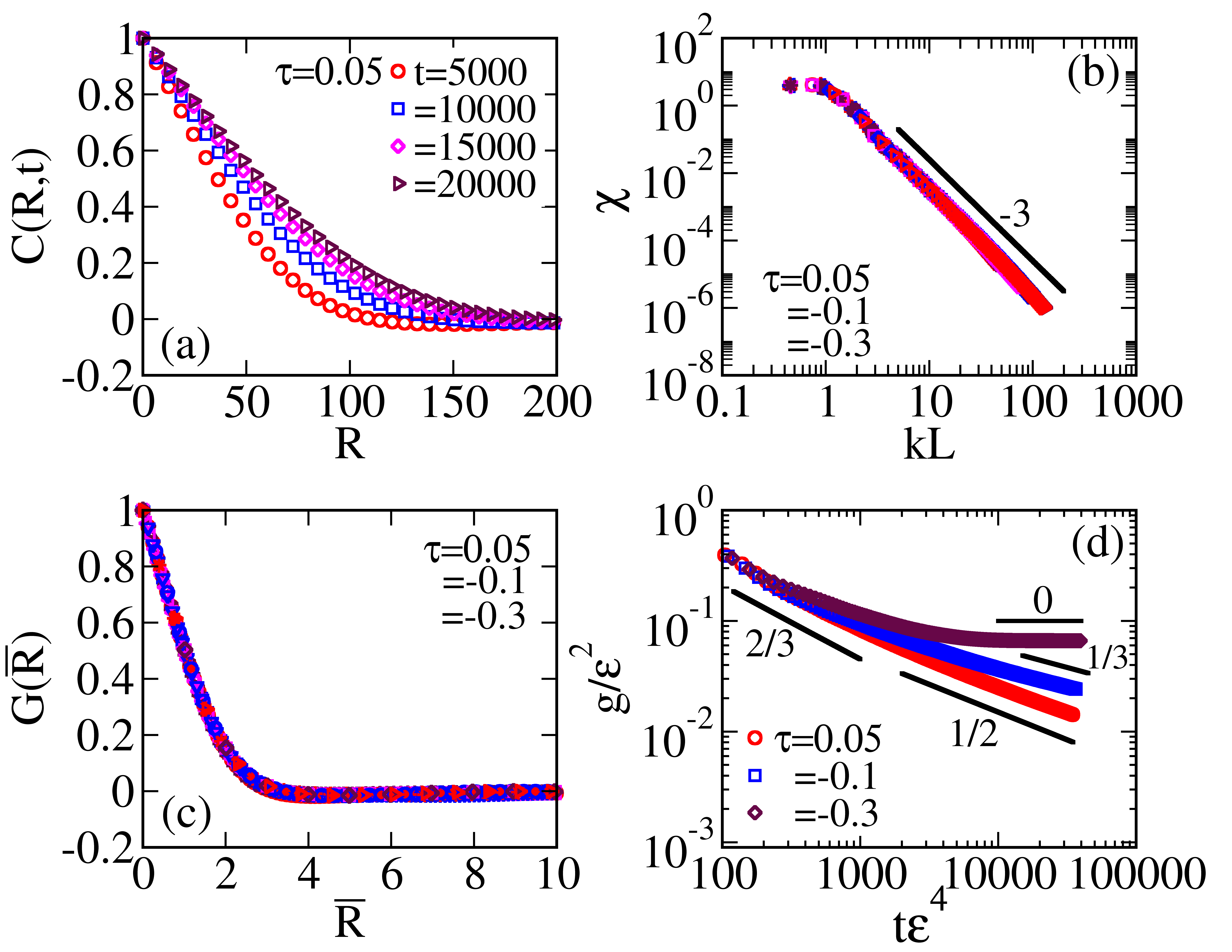
Figure 10: (Color online) Bales-Gooding OP correlations for deep quenches, including below the τ=0𝜏0\tau=0 spinodal: (a) For τ=0.05𝜏0.05\tau=0.05, data for C(R,t)𝐶𝑅𝑡C(R,t) versus R𝑅R for various times t𝑡t; (b) Porod’s Law behaviour in χ(kL)𝜒𝑘𝐿\chi(kL) versus scaled wave-vector kL(t)𝑘𝐿𝑡kL(t) showing data collapse in Fourier space, for all times, and temperatures ; (c) Dynamical scaling in G(R¯)𝐺¯𝑅G(\bar{R}) versus R¯R/L¯𝑅𝑅𝐿\bar{R}\equiv R/L showing data collapse for all times, and approximately for all temperatures; (d) Log-Log plot of scaled coarsening curvature g(t)/ε¯(τ)2𝑔𝑡¯𝜀superscript𝜏2g(t)/{\bar{\varepsilon}}(\tau)^{2} versus scaled time tε¯(τ)4𝑡¯𝜀superscript𝜏4t~{}{\bar{\varepsilon}}(\tau)^{4} with indicated exponents α=1/2,1/3,0𝛼12130\alpha=1/2,1/3,0, seen within the thsubscript𝑡t_{h}.

Figure 2(b) shows the CH case ordered-fraction nm(t)subscript𝑛𝑚𝑡n_{m}(t) versus scaled time t/tsc=tϵ2𝑡subscript𝑡sc𝑡superscriptitalic-ϵ2t/t_{\rm sc}=t\epsilon^{2}, where its slow rise for T𝑇T close to Tcsubscript𝑇𝑐T_{c} is due to critical slowing down near a second-order transition. As will be seen, these intermediate times can nonetheless show exponent behaviour.

Figure 3 shows snapshots of evolving relief plots of the OP e(r,t)𝑒𝑟𝑡e(\vec{r},t) versus position (x,y)𝑥𝑦(x,y), for early time evolutions for t=100,250,1500𝑡1002501500t=100,250,1500, and deep quenches. The strain textures or DW patterns, clearly coarsen with time.

Figure 4 again shows snapshots of coarsening, but now as evolving contour plots, for shallow, moderate and deep quenches. We will later consider several such quenches just below τ=+0.6,+0.3,+0.05𝜏0.60.30.05\tau=+0.6,+0.3,+0.05, corresponding to Δτ(T)τ(T)τ(T4)=0.1,0.5,0.8formulae-sequenceΔ𝜏𝑇𝜏𝑇𝜏subscript𝑇40.10.50.8\Delta\tau(T)\equiv\tau(T)-\tau(T_{4})=-0.1,-0.5,-0.8. The first row is for a shallow quench, to τ=0.6𝜏0.6\tau=0.6, and shows, in a background of e=0𝑒0e=0 austenite, many whorl-texture droplets at early times, like a DW vapour. The second and third rows are for moderate and deep quenches around τ=0.2,0.1𝜏0.20.1\tau=0.2,-0.1, with wandering martensite-martensite interfaces, like a DW liquid. For deep quenches, the coarsening seems to slow, or be arrested to form a DW Glass, as discussed later.

As a benchmark, we start with the familiar CH case, in 2D and with a scalar NOP=1subscript𝑁𝑂𝑃1N_{OP}=1 order parameter. Fig 5 shows the well-known results of dynamical scaling.

Figure 5(a) shows C(R,t)𝐶𝑅𝑡C(R,t) versus R𝑅R curves at different times for a given quench, with ϵ(T)=0.5italic-ϵ𝑇0.5\epsilon(T)=-0.5 shown. Extracting the coarsening length and re-plotting, we find (i) data collapse of different- time curves on to a common scaling curve C(R,t)=G(g(t)R)𝐶𝑅𝑡𝐺𝑔𝑡𝑅C(R,t)=G(g(t)R), for that quench; further, (ii) data collapse of different-quench scaling curves G(R¯)𝐺¯𝑅G(\bar{R}) onto a single T𝑇T-independent curve. This is consistent with (2.14), which predicted a OP-scaled CH dynamics would be independent of temperature. The curvature exponents are consistent with the literature, with a long-time exponent R1 of α=1/3𝛼13\alpha=1/3 and, for temperatures close to Tcsubscript𝑇𝑐T_{c}, an intermediate-time exponent R5 α=1/4𝛼14\alpha=1/4. Simulations in d=3𝑑3d=3, show R8 the same asymptotic α=1/3𝛼13\alpha=1/3 exponent, that is, thus independent of spatial dimension.

Figure 6 shows CH case log–log plots of the scaled curvature g/ε¯=g/|ϵ|1/2𝑔¯𝜀𝑔superscriptitalic-ϵ12g/{\bar{\varepsilon}}=g/|\epsilon|^{1/2} versus scaled time tε¯4=t|ϵ|2𝑡superscript¯𝜀4𝑡superscriptitalic-ϵ2t{\bar{\varepsilon}}^{4}=t|\epsilon|^{2}, showing data collapse, not only for all times, but also for all temperatures, as expected from the OP-scaled form of (2.14). Existing results R1 ; R8 ; R9 have temperature-independent exponents at intermediate-times where g(t)ξGL(T)>1𝑔𝑡subscript𝜉GL𝑇1g(t)\xi_{\rm GL}(T)>1 as α=1/4𝛼14\alpha=1/4; and a long times where gξGL(T)<1𝑔subscript𝜉GL𝑇1g\xi_{\rm GL}(T)<1 as the Lifshitz-Slyozov exponent of α=1/3𝛼13\alpha=1/3. Extracting exponent values from data (as for BG case of Appendix C), we find averaged exponents and standard deviations as

α=0.27±0.02;α=0.34±0.02,(4.1)formulae-sequence𝛼plus-or-minus0.270.02𝛼plus-or-minus0.340.024.1~{}~{}~{}\alpha=0.27\pm 0.02~{};~{}~{}\alpha=0.34\pm 0.02,~{}~{}~{}~{}~{}~{}~{}(4.1)

close to 1/4141/4 and 1/3131/3, as in previous work.

Turning to the BG case quenches, Bales and Gooding in 1D find a backward-bending phase boundary of inverse damping versus temperature. Figure 7 shows that in the 2D case, the phase diagram of inverse-damping Λ1/γsimilar-toΛ1𝛾\sqrt{\Lambda}\sim 1/\gamma versus temperature τ(T)𝜏𝑇\tau(T) also has the transition occurring at lower τ𝜏\tau, for decreasing damping. Below the boundary, the dilute initial seeds with small nmsubscript𝑛𝑚n_{m}, evolve to nm1subscript𝑛𝑚1n_{m}\rightarrow 1 (martensite), while above it, nm0subscript𝑛𝑚0n_{m}\rightarrow 0 (austenite). All quenches are to below the phase boundary.

For d=2𝑑2d=2 in previous Monte Carlo simulations of a related model, a complex textural energy was parametrized by a surrogate-droplet energy that was a universal inverted parabola versus a scaled evolving textural parameter R18 . As a check, our BG case dynamical evolutions were benchmarked against this energy parametrization R23 .

The BG case plots of Figs. 8-10 show numerical results analogous to the CH case, demonstrating dynamical scaling, for the three quench regimes each, just below τ=0.6,0.3,0.05𝜏0.60.30.05\tau=0.6,0.3,0.05, as mentioned. More in detail, all the Figures show the following: (a) correlations C(R,t)𝐶𝑅𝑡C(R,t) versus R𝑅R curves at different times, for quench to a given τ(T)𝜏𝑇\tau(T); (b) scaled structure factor χ(kL)𝜒𝑘𝐿{\chi}(kL), using the extracted L(t)𝐿𝑡L(t), versus k¯=kL¯𝑘𝑘𝐿\bar{k}=kL showing Porod’s tail behaviour of exponent -3 and Fourier data collapse; (c) dynamical scaling with data collapse of different-time curves on to a common scaling curve C(R,t)=G(g(t)R)𝐶𝑅𝑡𝐺𝑔𝑡𝑅C(R,t)=G(g(t)R), for that τ𝜏\tau quench. However, the scaling curves G(R¯)𝐺¯𝑅G(\bar{R}), are different for different τ𝜏\tau, especially for the shallow quenches of Fig. 8; while for deeper quenches of Figs. 9 and 10, the curves are closer. This is consistent with the OP-scaled result of (2.15), that shows a residual T𝑇T-dependence of the BG dynamics, through ηsc(T)=τ(T)/3ε¯(T)4subscript𝜂𝑠𝑐𝑇𝜏𝑇3¯𝜀superscript𝑇4\eta_{sc}(T)=\tau(T)/3{\bar{\varepsilon}}(T)^{4}, that is, insensitive to τ𝜏\tau at low temperatures. Also they show (d) log-log plots of the coarsening curvature versus time, showing different indicated exponents in different time windows, within the holding time thsubscript𝑡t_{h}.

Figure 8 shows α=2/3𝛼23\alpha=2/3; Fig. 9 shows α=2/3𝛼23\alpha=2/3 followed by 1/2121/2; Fig. 10 shows α=1/2𝛼12\alpha=1/2 followed by α=1/3𝛼13\alpha=1/3, and a peculiar flattening to ‘α=0𝛼0\alpha=0’ at low temperatures. The trapped curvature g0=0.1subscript𝑔00.1g_{0}=0.1 is not just a finite-size effect, as for our system sizes, g01/Lsys104much-greater-thansubscript𝑔01subscript𝐿syssimilar-tosuperscript104g_{0}\gg 1/L_{\rm sys}\sim 10^{-4} .

The exponent mean values and standard deviations, with simple arithmetic average over all temperatures, are

α=0.66±0.02and0.53±0.02,(4.2)𝛼plus-or-minus0.660.02a𝑛𝑑plus-or-minus0.530.024.2~{}~{}~{}~{}~{}\alpha=0.66\pm 0.02~{}~{}~{}{\text{a}nd}~{}~{}~{}~{}0.53\pm 0.02,~{}~{}~{}~{}~{}~{}~{}~{}~{}~{}~{}~{}~{}~{}~{}~{}~{}~{}~{}~{}~{}~{}(4.2)

that are close to α=2/3𝛼23\alpha=2/3 and α=1/2𝛼12\alpha=1/2. See Appendix C for a time-window procedure for extracting exponents.
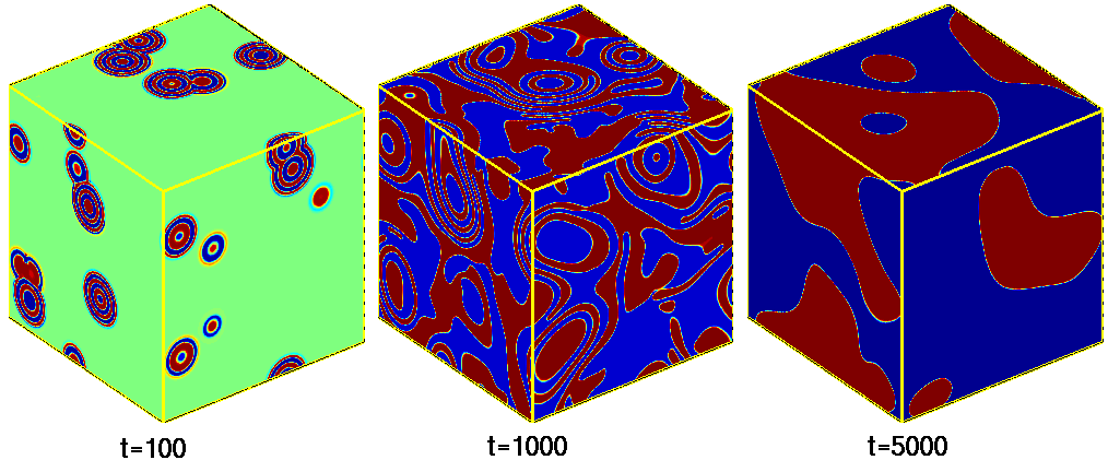
Refer to caption
Figure 11: (Color online) Contour plots of 3D strain evolutions: Snapshots for various times show the OP strain e(r,t)𝑒𝑟𝑡e({\vec{r}},t) evolving after a quench, in a system of size 5123superscript5123512^{3}.
Refer to caption
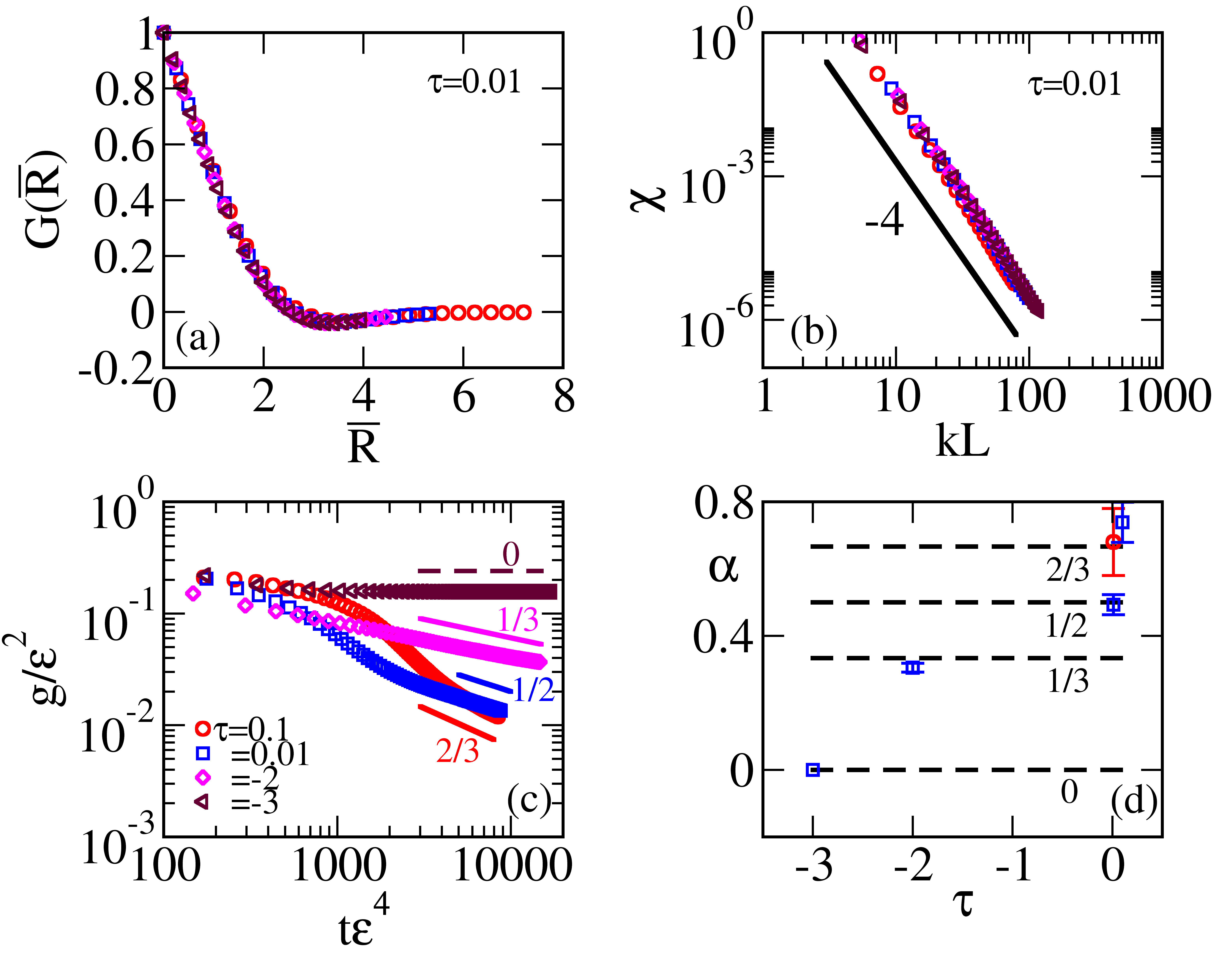
Figure 12: (Color online) Bales-Gooding OP correlations in 3D for τ=0.01𝜏0.01\tau=0.01 : (a) Dynamical scaling in G(R¯)𝐺¯𝑅G(\bar{R}) versus R¯R/L¯𝑅𝑅𝐿\bar{R}\equiv R/L for various times t𝑡t, showing data collapse in coordinate space; (b) Porod’s Law behaviour in χ(kL)𝜒𝑘𝐿\chi(kL) versus kL𝑘𝐿kL showing data collapse in Fourier space, with slope (d+NOP)=4𝑑subscript𝑁OP4-(d+N_{\rm OP})=-4; (c) Log-Log plot of scaled coarsening curvature g(t)/ε¯2𝑔𝑡superscript¯𝜀2g(t)/{\bar{\varepsilon}}^{2} versus scaled time tε¯4𝑡superscript¯𝜀4t\bar{\varepsilon}^{4} showing various indicated exponents; (d) Fitted exponent values α𝛼\alpha versus quench temperature τ𝜏\tau, showing that the 3D values close to 2/3,1/2,1/3,023121302/3,1/2,1/3,0 are the same as in 2D.

All this is for 2D. We have also considered 3D coarsening textures, as shown in surface contour plots of Fig. 11. The 3D case also shows dynamical scaling as shown in Fig. 12, with the Porod’s law exponent now (d+1)=4𝑑14-(d+1)=-4, and data collapse as before. For successively deeper quenches, the exponents are found to be again close to α=2/3,1/2,1/3,0𝛼2312130\alpha=2/3,1/2,1/3,0, so the coarsening exponents are independent of spatial dimension.

V Correlation-function Dynamics and Dynamical Scaling

The exponent behaviour has been extracted from various OP dynamics by many authors R1 ; R5 ; R6 ; R11 , including Siggia through insightful heuristic arguments; Bray and Rutenberg through matching global and local dissipation; Ohta, Jasnow, and Kawasaki; Bray, and Puri, and Mazenko, through a fluctuating domain wall approach; and Langer et al. through a self-consistent truncation of correlation function dynamics. We suggest a complementary, and systematic curvature kinetics approach, to extract exponent behaviour.

In our theoretical analysis, we will use throughout, the OP-scaled form of the CH and BG dynamics, that fully or mostly, scales out the OP temperature dependence. We first obtain the dynamics of the two-point OP-OP correlation as done previously, elsewhere R5 .

V.1 Evolution of correlation function

The correlation function dynamics can be derived R5 ; R24 . from a given order parameter dynamics, such as the OP-scaled dynamics of (2.14) and (2.15). From (2.14), the “mass-conserving” Cahn-Hilliard correlation function dynamics is

tC(R,t)=R2C(μ)(R,t).(5.1)formulae-sequence𝑡𝐶𝑅𝑡superscriptsubscript𝑅2superscript𝐶𝜇𝑅𝑡5.1\frac{\partial}{\partial t}C(R,t)={\vec{\nabla}_{\vec{R}}}^{2}C^{(\mu)}(R,t).~{}~{}~{}(5.1)

From (2.15) we similarly get a “momentum-conserving” Bales-Gooding correlation dynamics,

Λ2t2C(R,t)=R2[C(μ)(R,t)+C(R,t)t].(5.2)formulae-sequenceΛsuperscript2superscript𝑡2𝐶𝑅𝑡superscriptsubscript𝑅2delimited-[]superscript𝐶𝜇𝑅𝑡𝐶𝑅𝑡𝑡5.2\Lambda\frac{\partial^{2}}{\partial t^{2}}C(R,t)={\vec{\nabla}_{\vec{R}}}^{2}\left[~{}C^{(\mu)}(R,t)+\frac{\partial C(R,t)}{\partial t}\right].~{}~{}~{}(5.2)

The chemical potential-order parameter correlation or μOP𝜇O𝑃\mu-{\text{O}P} correlation of (3.3), has separate Landau and Ginzburg contributions,

C(μ)(R,t)C(μL)(R,t)+C(μG)(R,t),(5.3)superscript𝐶𝜇𝑅𝑡superscript𝐶subscript𝜇𝐿𝑅𝑡superscript𝐶subscript𝜇𝐺𝑅𝑡5.3C^{(\mu)}(R,t)\equiv{C}^{(\mu_{L})}(R,t)+{C}^{(\mu_{G})}(R,t),~{}~{}~{}(5.3)

where the Ginzburg term depends directly on the OP-OP correlation,

C(μG)(R,t)[12fGe(r,t)]e(r,t)superscript𝐶subscript𝜇𝐺𝑅𝑡delimited-⟨⟩delimited-[]12subscript𝑓𝐺𝑒𝑟𝑡𝑒superscript𝑟𝑡{C}^{(\mu_{G})}(R,t)\equiv\left\langle\left[\frac{1}{2}\frac{\partial f_{G}}{\partial e(\vec{r},t)}\right]e(\vec{r^{\prime}},t)\right\rangle
=R2C(R,t),(5.4a)absentsuperscriptsubscript𝑅2𝐶𝑅𝑡5.4𝑎=-{\vec{\nabla}_{\vec{R}}}^{2}C(R,t),~{}~{}~{}(5.4a)

while the Landau contribution carries the higher powers of the strain

C(μL)(R,t)[12fLe(r,t)]e(r,t)superscript𝐶subscript𝜇𝐿𝑅𝑡delimited-⟨⟩delimited-[]12subscript𝑓𝐿𝑒𝑟𝑡𝑒superscript𝑟𝑡{C}^{(\mu_{L})}(R,t)\equiv\left\langle\left[\frac{1}{2}\frac{\partial f_{L}}{\partial e(\vec{r},t)}\right]e(\vec{r^{\prime}},t)\right\rangle
f0(e(r,t))e(r,t)e(r,t),(5.4b)absentdelimited-⟨⟩subscript𝑓0𝑒𝑟𝑡𝑒𝑟𝑡𝑒superscript𝑟𝑡5.4𝑏\equiv-\left\langle f_{0}(e(\vec{r},t))e(\vec{r},t)e(\vec{r^{\prime}},t)\right\rangle,~{}~{}~{}(5.4b)

where the BG-case scaled polynomial factors f0(e)subscript𝑓0𝑒f_{0}(e) have been given earlier.

V.2 Dynamic scaling ansatz

We assume the correlation functions have a dynamic scaling form, and insert this as an ansatz or trial solution,

C(R,t)=G(R¯),(5.5a)𝐶𝑅𝑡𝐺¯𝑅5.5𝑎C(R,t)=G(\bar{R}),~{}~{}(5.5a)

where the argument of the scaling function is henceforth

R¯g(t)R.(5.5b)formulae-sequence¯𝑅𝑔𝑡𝑅5.5𝑏{\bar{R}}\equiv g(t)R.~{}~{}(5.5b)

For the Landau part of μlimit-from𝜇\mu-OP correlation function with three lengths ξ0,R,Lsubscript𝜉0𝑅𝐿\xi_{0},R,L,we can similarly assume a general scaling form in ratios R/L(t),ξ0/L(t)𝑅𝐿𝑡subscript𝜉0𝐿𝑡R/L(t),\xi_{0}/L(t):

C(μL)(R,t)=(gξ0)δLG(μL)(R¯,gξ0),(5.6)superscript𝐶subscript𝜇𝐿𝑅𝑡superscript𝑔subscript𝜉0subscript𝛿𝐿superscript𝐺subscript𝜇𝐿¯𝑅𝑔subscript𝜉05.6{C}^{(\mu_{L})}(R,t)=(g\xi_{0})^{\delta_{L}}G^{(\mu_{L})}(\bar{R},g\xi_{0}),~{}(5.6)

where G(μL)superscript𝐺subscript𝜇𝐿G^{(\mu_{L})} is some scaling function, and δLsubscript𝛿𝐿\delta_{L} some universal exponent.

The model dynamics can be written in terms of R¯¯𝑅{\bar{R}} derivatives of the scaling functions, and time-derivatives of the curvature g(t)𝑔𝑡g(t).

The Laplacians are derivatives in R¯¯𝑅\bar{R}, with no angular derivative surviving, when acting on isotropic functions

R2=g2D^;D^[2R¯2+(d1)R¯R¯].(5.7)formulae-sequenceformulae-sequencesuperscriptsubscript𝑅2superscript𝑔2^𝐷^𝐷delimited-[]superscript2superscript¯𝑅2𝑑1¯𝑅¯𝑅5.7\vec{\nabla}_{\vec{R}}^{2}=g^{2}{\hat{D}}~{};{\hat{D}}\equiv\left[\frac{\partial^{2}}{\partial{\bar{R}}^{2}}+\frac{(d-1)}{\bar{R}}\frac{\partial}{\partial{\bar{R}}}\right].~{}(5.7)

The time derivatives are

G(gR)t={g˙g}R¯G(R¯);(5.8a)𝐺𝑔𝑅𝑡˙𝑔𝑔¯𝑅superscript𝐺¯𝑅5.8𝑎\frac{\partial G(gR)}{\partial t}=\left\{\frac{\dot{g}}{g}\right\}{\bar{R}}G^{\prime}({\bar{R}});~{}~{}~{}(5.8a)
2G(gR)t2={g¨g}R¯G(R¯)+{g˙g}2R¯2G′′(R¯),(5.8b)superscript2𝐺𝑔𝑅superscript𝑡2¨𝑔𝑔¯𝑅superscript𝐺¯𝑅superscript˙𝑔𝑔2superscript¯𝑅2superscript𝐺′′¯𝑅5.8𝑏\frac{\partial^{2}G(gR)}{\partial t^{2}}=\left\{\frac{\ddot{g}}{g}\right\}{\bar{R}}G^{\prime}(\bar{R})+\left\{\frac{\dot{g}}{g}\right\}^{2}{\bar{R}}^{2}G^{\prime\prime}(\bar{R}),~{}~{}(5.8b)

where primes denote derivatives GdG/dR¯,G′′d2G/dR¯2formulae-sequencesuperscript𝐺𝑑𝐺𝑑¯𝑅superscript𝐺′′superscript𝑑2𝐺𝑑superscript¯𝑅2G^{\prime}\equiv dG/d{\bar{R}},G^{\prime\prime}\equiv d^{2}G/d{\bar{R}}^{2} and so on. Note the prefactors of the curvature time-derivatives contain G(R¯)superscript𝐺¯𝑅G^{\prime}(\bar{R}), which is slowly varying at its turning points G′′(R¯=R¯0)=0superscript𝐺′′¯𝑅subscript¯𝑅00G^{\prime\prime}(\bar{R}=\bar{R}_{0})=0.

The Cahn-Hilliard (CH) dynamics is, setting ξ0=1subscript𝜉01\xi_{0}=1,

{g˙g}R¯G(R¯)=gδL[g2D^G(μL)(R¯,g)]g4[D^]2G.(5.9a)formulae-sequence˙𝑔𝑔¯𝑅superscript𝐺¯𝑅superscript𝑔subscript𝛿𝐿delimited-[]superscript𝑔2^𝐷superscript𝐺subscript𝜇𝐿¯𝑅𝑔superscript𝑔4superscriptdelimited-[]^𝐷2𝐺5.9𝑎\left\{\frac{\dot{g}}{g}\right\}{\bar{R}}G^{\prime}({\bar{R}})=g^{\delta_{L}}\left[g^{2}{\hat{D}}{G}^{(\mu_{L})}({\bar{R}},g)\right]-g^{4}\left[{\hat{D}}\right]^{2}G~{}.~{}~{}(5.9a)

The Bales-Gooding (BG) dynamics is

Λ[{g¨g}R¯G(R¯)+{g˙g}2R¯2G′′(R¯)]=Λdelimited-[]¨𝑔𝑔¯𝑅superscript𝐺¯𝑅superscript˙𝑔𝑔2superscript¯𝑅2superscript𝐺′′¯𝑅absent\Lambda\left[\left\{\frac{\ddot{g}}{g}\right\}{\bar{R}}G^{\prime}(\bar{R})+\left\{\frac{\dot{g}}{g}\right\}^{2}{\bar{R}}^{2}G^{\prime\prime}(\bar{R})\right]=
g2+δL[D^G(μL)(R¯)]g4[D^2G]+g2{g˙g}D^(R¯G).(5.9b)formulae-sequencesuperscript𝑔2subscript𝛿𝐿delimited-[]^𝐷superscript𝐺subscript𝜇𝐿¯𝑅superscript𝑔4delimited-[]superscript^𝐷2𝐺superscript𝑔2˙𝑔𝑔^𝐷¯𝑅superscript𝐺5.9𝑏g^{2+\delta_{L}}\left[{\hat{D}}G^{(\mu_{L})}({\bar{R}})\right]-g^{4}\left[{\hat{D}}^{2}G\right]+g^{2}\left\{\frac{\dot{g}}{g}\right\}{\hat{D}}({\bar{R}}G^{\prime}).~{}~{}(5.9b)

The derivative operators of (5.7) yield

D^G(μL)=1R¯2[(d1)R¯G(μL)+R¯2G(μL)′′];(5.10a)^𝐷superscript𝐺subscript𝜇𝐿1superscript¯𝑅2delimited-[]𝑑1¯𝑅superscriptsuperscript𝐺subscript𝜇𝐿superscript¯𝑅2superscriptsuperscript𝐺subscript𝜇𝐿′′5.10𝑎{\hat{D}}G^{(\mu_{L})}=\frac{1}{{\bar{R}}^{2}}\left[(d-1){\bar{R}}{G^{(\mu_{L})}}^{\prime}+{\bar{R}}^{2}{G^{(\mu_{L})}}^{\prime\prime}\right]~{};~{}~{}(5.10a)
D^2G=1R¯4[(3d)(d1)(R¯GR¯2G′′){\hat{D}}^{2}G=\frac{1}{{\bar{R}}^{4}}[(3-d)(d-1)({\bar{R}}G^{\prime}-{\bar{R}}^{2}G^{\prime\prime})
+2(d1)R¯3G′′′+R¯4G′′′′];(5.10b)+2(d-1){{\bar{R}}^{3}}G^{\prime\prime\prime}+{\bar{R}}^{4}G^{\prime\prime\prime\prime}]~{};~{}~{}~{}~{}~{}~{}(5.10b)
D^[R¯G]=1R¯2[(d1)R¯G+(d+1)R¯2G′′+R¯3G′′′].(5.10c)formulae-sequence^𝐷delimited-[]¯𝑅superscript𝐺1superscript¯𝑅2delimited-[]𝑑1¯𝑅superscript𝐺𝑑1superscript¯𝑅2superscript𝐺′′superscript¯𝑅3superscript𝐺′′′5.10𝑐{\hat{D}}\left[{\bar{R}}G^{\prime}\right]=\frac{1}{{\bar{R}}^{2}}\left[(d-1){\bar{R}}G^{\prime}+(d+1){\bar{R}}^{2}G^{\prime\prime}+{\bar{R}}^{3}G^{\prime\prime\prime}\right].~{}(5.10c)

Collecting terms above, and dividing through by R¯G(R¯)¯𝑅superscript𝐺¯𝑅{\bar{R}}G^{{}^{\prime}}({\bar{R}})~{}, we have for the CH case,

g˙g=J3(R¯)g2+δL+J4(R¯)g4;(5.11a)˙𝑔𝑔subscript𝐽3¯𝑅superscript𝑔2subscript𝛿𝐿subscript𝐽4¯𝑅superscript𝑔45.11𝑎\frac{-\dot{g}}{g}=J_{3}(\bar{R})g^{2+\delta_{L}}+J_{4}(\bar{R})g^{4};~{}~{}(5.11a)

and for the BG case,

Λ[g¨g+I2(R¯){g˙g}2]+K1(R¯){g˙g}g2Λdelimited-[]¨𝑔𝑔subscript𝐼2¯𝑅superscript˙𝑔𝑔2subscript𝐾1¯𝑅˙𝑔𝑔superscript𝑔2-\Lambda\left[\frac{\ddot{g}}{g}+I_{2}(\bar{R})\left\{\frac{\dot{g}}{g}\right\}^{2}\right]+K_{1}(\bar{R})\left\{\frac{-\dot{g}}{g}\right\}g^{2}
=J3(R¯)g2+δL+J4(R¯)g4.(5.11b)formulae-sequenceabsentsubscript𝐽3¯𝑅superscript𝑔2subscript𝛿𝐿subscript𝐽4¯𝑅superscript𝑔45.11𝑏=J_{3}(\bar{R})g^{2+\delta_{L}}+J_{4}(\bar{R})g^{4}.~{}~{}(5.11b)

Here Jnsubscript𝐽𝑛J_{n} are R¯¯𝑅\bar{R}-dependent coefficients of powers gnsuperscript𝑔𝑛g^{n} of the force terms, while K1(R¯)subscript𝐾1¯𝑅K_{1}(\bar{R}) is a coefficient of the kinetic damping term. (The Landau term coefficient is called J3(R¯)subscript𝐽3¯𝑅J_{3}(\bar{R}), as δL=1subscript𝛿𝐿1\delta_{L}=1, later.)

The coefficients in (5.11) are

K1(R¯)[1R¯2][(d1)+(d+1)I2+I3];(5.12a)subscript𝐾1¯𝑅delimited-[]1superscript¯𝑅2delimited-[]𝑑1𝑑1subscript𝐼2subscript𝐼35.12𝑎K_{1}(\bar{R})\equiv\left[\frac{-1}{{{\bar{R}}}^{2}}\right]\left[(d-1)+(d+1)I_{2}+I_{3}\right]~{};~{}~{}(5.12a)
J3(R¯,T)[1R¯2][(d1)R¯G(μL)+R¯2G(μL)′′]/R¯G;(5.12b)subscript𝐽3¯𝑅𝑇delimited-[]1superscript¯𝑅2delimited-[]𝑑1¯𝑅superscriptsuperscript𝐺subscript𝜇𝐿superscript¯𝑅2superscriptsuperscript𝐺subscript𝜇𝐿′′¯𝑅superscript𝐺5.12𝑏J_{3}(\bar{R},T)\equiv\left[\frac{-1}{{\bar{R}}^{2}}\right][(d-1){\bar{R}}{G^{(\mu_{L})}}^{\prime}+{\bar{R}}^{2}{G^{(\mu_{L})}}^{\prime\prime}]/{\bar{R}}G^{\prime}~{};(5.12b)
J4(R¯)[1R¯4][(3d)(d1)(1I2)+2(d1)I3+I4],(5.12c)subscript𝐽4¯𝑅delimited-[]1superscript¯𝑅4delimited-[]3𝑑𝑑11subscript𝐼22𝑑1subscript𝐼3subscript𝐼45.12𝑐J_{4}(\bar{R})\equiv\left[\frac{1}{{\bar{R}}^{4}}\right]\left[(3-d)(d-1)(1-I_{2})+2(d-1)I_{3}+I_{4}\right],~{}(5.12c)

with all in terms of the derivative ratios of G(R¯)𝐺¯𝑅G(\bar{R}),

I2R¯2G(μL)′′(R¯)R¯G(R¯);subscript𝐼2superscript¯𝑅2superscriptsuperscript𝐺subscript𝜇𝐿′′¯𝑅¯𝑅superscript𝐺¯𝑅I_{2}\equiv\frac{{{\bar{R}}}^{2}{G^{(\mu_{L})}}^{\prime\prime}({\bar{R}})}{{{\bar{R}}}G^{\prime}({\bar{R}})}~{};
I3(R¯)R¯3G′′′(R¯)R¯G(R¯);I4(R¯)R¯4G′′′′(R¯)R¯G(R¯).(5.13)formulae-sequenceformulae-sequencesubscript𝐼3¯𝑅superscript¯𝑅3superscript𝐺′′′¯𝑅¯𝑅superscript𝐺¯𝑅subscript𝐼4¯𝑅superscript¯𝑅4superscript𝐺′′′′¯𝑅¯𝑅superscript𝐺¯𝑅5.13~{}I_{3}(\bar{R})\equiv\frac{{{\bar{R}}}^{3}G^{\prime\prime\prime}({\bar{R}})}{{{\bar{R}}}G^{\prime}({\bar{R}})}~{};I_{4}(\bar{R})\equiv\frac{{{\bar{R}}}^{4}G^{\prime\prime\prime\prime}({\bar{R}})}{{{\bar{R}}}G^{\prime}({\bar{R}})}~{}.~{}~{}(5.13)

So far, this is formally exact, with the only input being a dynamical-scaling trial solution. The coefficient J3subscript𝐽3J_{3} contains the yet unspecified G(μL)superscript𝐺subscript𝜇𝐿G^{(\mu_{L})}, that carries the higher-order correlations in the OP. Its further evolution equations would induce a dynamically coupled, infinite hierarchy R5 . A closure approximation is needed, and there must be a coefficient evaluation at some physically motivated, expanding-front value of R¯¯𝑅\bar{R}.

V.3 Approximations

a) Closure Approximation:

The correlation between the Landau chemical potential and the OP is

C(μL)=f0(e(r,t))e(r,t)e(r,t).(5.14a)formulae-sequencesuperscript𝐶subscript𝜇𝐿delimited-⟨⟩subscript𝑓0𝑒𝑟𝑡𝑒𝑟𝑡𝑒superscript𝑟𝑡5.14𝑎C^{(\mu_{L})}=-\left\langle f_{0}(e(\vec{r},t))~{}e(\vec{r},t)e(\vec{r^{\prime}},t)\right\rangle.~{}~{}(5.14a)

and the factor f0(e)subscript𝑓0𝑒f_{0}(e) carries higher order powers of e𝑒e, that induce the correlation hierarchy. For a uniform or bulk order parameter e=±1𝑒plus-or-minus1e=\pm 1, the Landau part of the chemical potential vanishes, μLfL/e=ef0(e)=0similar-tosubscript𝜇𝐿subscript𝑓𝐿𝑒𝑒subscript𝑓0𝑒0\mu_{L}\sim\partial f_{L}/\partial e=-ef_{0}(e)=0. The correlation C(μL)(R,t)superscript𝐶subscript𝜇𝐿𝑅𝑡{C}^{(\mu_{L})}(R,t) has contributions only from the non-uniform OP regions around domain walls, where f0(e)0subscript𝑓0𝑒0f_{0}(e)\neq 0 over a thickness ξ0subscript𝜉0\xi_{0} between the competing bulk values. Thus C(μL)superscript𝐶subscript𝜇𝐿{C}^{(\mu_{L})} is a correlation between an OP and many possible DW. It decreases for decreasing DW thickness ξ0subscript𝜉0\xi_{0}, and C(gξ0)δLsimilar-to𝐶superscript𝑔subscript𝜉0subscript𝛿𝐿C\sim(g\xi_{0})^{\delta_{L}} as in (5.6). Interpreting the scaling function G(μL)superscript𝐺subscript𝜇𝐿G^{(\mu_{L})} as a correlation between the OP and a single DW the prefactor is then the probability of finding a DW, enabling an estimate of δLsubscript𝛿𝐿\delta_{L}.

In a coarsening volume L(t)2𝐿superscript𝑡2L(t)^{2}, the probability of finding a scalar-OP DW is roughly (ξ0L)/L2=ξ0/L=ξ0gsubscript𝜉0𝐿superscript𝐿2subscript𝜉0𝐿subscript𝜉0𝑔(\xi_{0}L)/L^{2}=\xi_{0}/L=\xi_{0}g. The exponent in (5.6) for NOP=1subscript𝑁OP1N_{\rm OP}=1 is then δL=1subscript𝛿𝐿1\delta_{L}=1.

As Bray R1 has noted, for general number of OP components, and in d𝑑d spatial dimensions, the vanishing at a DW of all the NOPsubscript𝑁OPN_{\rm OP} components, corresponds to a ‘surface’ of reduced dimension dNOP>0𝑑subscript𝑁OP0d-N_{\rm OP}>0. Thus more generally, in a coarsening volume Ldsuperscript𝐿𝑑L^{d}, the probability of finding a DW is roughly (ξ0NOPLdNOP)/Ld=(ξ0/L)NOP=(ξ0g)NOPsuperscriptsubscript𝜉0subscript𝑁OPsuperscript𝐿𝑑subscript𝑁OPsuperscript𝐿𝑑superscriptsubscript𝜉0𝐿subscript𝑁OPsuperscriptsubscript𝜉0𝑔subscript𝑁OP(\xi_{0}^{N_{\rm OP}}L^{d-N_{\rm OP}})/L^{d}=(\xi_{0}/L)^{N_{\rm OP}}=(\xi_{0}g)^{N_{\rm OP}}. The exponent for general NOPsubscript𝑁OPN_{\rm OP} is then δL=NOPsubscript𝛿𝐿subscript𝑁OP\delta_{L}=N_{\rm OP}, and (5.6) is taken as

C(μL)(R,t)=(gξ0)NOPG(μL)(R¯,gξ0).(5.14b)formulae-sequencesuperscript𝐶subscript𝜇𝐿𝑅𝑡superscript𝑔subscript𝜉0subscript𝑁OPsuperscript𝐺subscript𝜇𝐿¯𝑅𝑔subscript𝜉05.14𝑏{C}^{(\mu_{L})}(R,t)=(g\xi_{0})^{N_{\rm OP}}G^{(\mu_{L})}(\bar{R},g\xi_{0}).~{}~{}~{}(5.14b)

We make a simple closure approximation for the domain-wall scaling function G(μL)(R¯,gξ0)superscript𝐺subscript𝜇𝐿¯𝑅𝑔subscript𝜉0G^{(\mu_{L})}(\bar{R},g\xi_{0}). To leading order in gξ0𝑔subscript𝜉0g\xi_{0}, we take G(μL)(R¯,gξ0)G(μL)(R¯,0)similar-to-or-equalssuperscript𝐺subscript𝜇𝐿¯𝑅𝑔subscript𝜉0superscript𝐺subscript𝜇𝐿¯𝑅0G^{(\mu_{L})}(\bar{R},g\xi_{0})\simeq G^{(\mu_{L})}(\bar{R},0). (However in Section VI, we will consider possible higher curvature corrections in gξ0𝑔subscript𝜉0g\xi_{0} from G(μL)(R¯,gξ0)superscript𝐺subscript𝜇𝐿¯𝑅𝑔subscript𝜉0G^{(\mu_{L})}(\bar{R},g\xi_{0}), in a toy model for coarsening arrest.) We then replace the DW factor f0(e)subscript𝑓0𝑒f_{0}(e) by its spatial average f¯0(T)=f0(e(r))subscript¯𝑓0𝑇delimited-⟨⟩subscript𝑓0𝑒𝑟{\bar{f}}_{0}(T)=\langle f_{0}(e(\vec{r}))\rangle. This yields, as in Appendix A,

G(μL)(R¯,gξ0)G(μL)(R¯,0)=f¯0(T)G(R¯).(5.14c)formulae-sequencesimilar-to-or-equalssuperscript𝐺subscript𝜇𝐿¯𝑅𝑔subscript𝜉0superscript𝐺subscript𝜇𝐿¯𝑅0subscript¯𝑓0𝑇𝐺¯𝑅5.14𝑐G^{(\mu_{L})}(\bar{R},g\xi_{0})\simeq G^{(\mu_{L})}(\bar{R},0)=-{\bar{f}}_{0}(T)G(\bar{R}).~{}~{}(5.14c)

Thus reasonably, G(μL)superscript𝐺subscript𝜇𝐿G^{(\mu_{L})} has the same R¯¯𝑅\bar{R} dependence as G𝐺G, as also holds in other approximations R5 .

Inserting this closure approximation into the Landau term coefficient of (5.12b),

J3(R¯)f¯0(T)R¯2[(d1)+I2(R¯)].(5.15)formulae-sequencesimilar-to-or-equalssubscript𝐽3¯𝑅subscript¯𝑓0𝑇superscript¯𝑅2delimited-[]𝑑1subscript𝐼2¯𝑅5.15~{}J_{3}(\bar{R})\simeq\frac{{\bar{f}}_{0}(T)}{{\bar{R}}^{2}}\left[(d-1)+I_{2}(\bar{R})\right]~{}.~{}(5.15)

b) Coefficient evaluations

The correlation-function dynamics of (5.11) is now closed, but has a peculiar form, of an equation nonlinear in the curvature g(t)𝑔𝑡g(t) and its time derivatives; with coefficients linear in G(R¯)𝐺¯𝑅G(\bar{R}) and its scaled space derivatives.

The coefficients are evaluated at some constant separation R¯¯𝑅\bar{R}. As the slope G(R¯)superscript𝐺¯𝑅G^{\prime}(\bar{R}) is a prefactor in the kinetic terms, it is natural to focus on where it is slowly varying, at its own turning point, G′′(R¯0)=0superscript𝐺′′subscript¯𝑅00G^{\prime\prime}({\bar{R}}_{0})=0. This defines a dominant curvature front R=R¯0L(t)𝑅subscript¯𝑅0𝐿𝑡R={\bar{R}}_{0}L(t). For both CH and BG dynamics, G(R¯)𝐺¯𝑅G(\bar{R}) first has a minimum (G′′>0superscript𝐺′′0G^{\prime\prime}>0), and then a maximum (G′′<0superscript𝐺′′0G^{\prime\prime}<0), so this point where G′′=0superscript𝐺′′0G^{\prime\prime}=0 is somewhere in between. We evaluate all coefficients at the first turning point R¯=R¯0¯𝑅subscript¯𝑅0\bar{R}={\bar{R}}_{0} of G(R¯)superscript𝐺¯𝑅G^{\prime}(\bar{R}), that is also a non-stationary inflection point of the scaled correlation G(R¯)𝐺¯𝑅G(\bar{R}).

With G′′(R¯0)=0superscript𝐺′′subscript¯𝑅00G^{\prime\prime}({\bar{R}}_{0})=0 and hence I2(R¯0)=0subscript𝐼2subscript¯𝑅00I_{2}({\bar{R}}_{0})=0, the coefficients are

K10K1(R¯0)=[1R¯02][I3(R¯0)+(d1)];(5.16a)formulae-sequencesubscript𝐾10subscript𝐾1subscript¯𝑅0delimited-[]1superscriptsubscript¯𝑅02delimited-[]subscript𝐼3subscript¯𝑅0𝑑15.16𝑎K_{10}\equiv K_{1}({\bar{R}}_{0})=\left[\frac{-1}{{{\bar{R}}_{0}}^{2}}\right]\left[I_{3}(\bar{R}_{0})+(d-1)\right]~{};~{}~{}(5.16a)
J30J3(R¯0)=f¯0(T)(d1)R¯02;(5.16b)formulae-sequencesubscript𝐽30subscript𝐽3subscript¯𝑅0subscript¯𝑓0𝑇𝑑1superscriptsubscript¯𝑅025.16𝑏J_{30}\equiv J_{3}({\bar{R}}_{0})=\frac{{\bar{f}}_{0}(T)~{}(d-1)}{{\bar{R}_{0}}^{2}}~{};~{}~{}~{}(5.16b)
J40J4(R¯0)subscript𝐽40subscript𝐽4subscript¯𝑅0J_{40}\equiv J_{4}({\bar{R}}_{0})
=[1R¯04][I4(R¯0)+2(d1)I3(R¯0)+(3d)(d1)].(5.16c)formulae-sequenceabsentdelimited-[]1superscriptsubscript¯𝑅04delimited-[]subscript𝐼4subscript¯𝑅02𝑑1subscript𝐼3subscript¯𝑅03𝑑𝑑15.16𝑐=\left[\frac{1}{{\bar{R}_{0}}^{4}}\right]\left[I_{4}(\bar{R}_{0})+2(d-1)I_{3}(\bar{R}_{0})+(3-d)(d-1)\right].~{}(5.16c)

Note that I2=0subscript𝐼20I_{2}=0 in the inertial term of (5.8b), suppresses nonlinearities, leaving just a curvature acceleration, Λg¨/gsimilar-toabsentΛ¨𝑔𝑔\sim\Lambda\ddot{g}/g. Fits to G(R¯)𝐺¯𝑅G(\bar{R}) in Appendix B yield R¯0>1subscript¯𝑅01{\bar{R}}_{0}>1.

An alternative, and equivalent choice for coefficient evaluation is where the OP gradient-gradient correlation, or effective DW-DW correlation

Γ(R¯)g2re(r,t).re(r,t)(5.17)\Gamma(\bar{R})\equiv g^{-2}\langle\nabla_{\vec{r}}~{}e(\vec{r},t).\nabla_{\vec{r^{\prime}}}~{}e(\vec{r^{\prime}},t)\rangle~{}(5.17)

flattens to zero. Fig 15d of Appendix B shows that this flattening occurs near the previous choice, of the first inflection point R¯/R¯0=1¯𝑅subscript¯𝑅01{\bar{R}}/{\bar{R}}_{0}=1. This gives a physical justification to our evaluation choice.

The simple approximations made here are solely for the limited purpose of determining the now-constant coefficients, of a curvature kinetics.

VI Curvature Kinetics

The dynamics is now in terms of g(t)𝑔𝑡g(t) only, and can yield exponent behaviour for appropriate coefficient signs; with possible crossovers in time between these exponents.

The curvature kinetics, derived from a given order parameter dynamics, yields five main results.
i) There are time regimes where the curvatures decay as single power laws in time g1/tαsimilar-to𝑔1superscript𝑡𝛼g\sim 1/t^{\alpha}.
ii) The exponents α𝛼\alpha are ratios of integers, induced directly from the integer powers of the curvatures, in each derived kinetics.
iii) In addition to the long-time exponents, there can also be different exponent behaviour at intermediate times, from two different force terms sequentially balancing the kinetic term.
iv) The exponents are manifestly independent of spatial dimension d𝑑d that can be scaled out, but can depend on the number of order parameter components NOPsubscript𝑁OPN_{\rm OP}.
v) The scaled kinetics can be solved analytically in some cases, providing a universal scaling function of curvature versus time.

The curvature kinetics for the CH case is

g˙g=J30g2+NOP+J40g4.(6.1)formulae-sequence˙𝑔𝑔subscript𝐽30superscript𝑔2subscript𝑁OPsubscript𝐽40superscript𝑔46.1\frac{-\dot{g}}{g}=J_{30}g^{2+N_{\rm OP}}+J_{40}g^{4}.~{}~{}(6.1)

The curvature kinetics for the BG case is,

Λ[g¨g]+K10{g˙g}g2Λdelimited-[]¨𝑔𝑔subscript𝐾10˙𝑔𝑔superscript𝑔2-\Lambda\left[\frac{\ddot{g}}{g}\right]+K_{10}\left\{\frac{-\dot{g}}{g}\right\}g^{2}
=J30g2+NOP+J40g4.(6.2)formulae-sequenceabsentsubscript𝐽30superscript𝑔2subscript𝑁OPsubscript𝐽40superscript𝑔46.2=J_{30}g^{2+N_{\rm OP}}+J_{40}g^{4}.~{}~{}(6.2)

We now scale times and curvatures in crossover values tcr,gcrsubscript𝑡crsubscript𝑔crt_{\rm cr},g_{\rm cr}, and define

t¯t/tcr;g¯g/gcr.(6.3)formulae-sequenceformulae-sequence¯𝑡𝑡subscript𝑡cr¯𝑔𝑔subscript𝑔cr6.3\bar{t}\equiv t/t_{\rm cr}~{};~{}~{}\bar{g}\equiv g/g_{\rm cr}.~{}~{}(6.3)

The ’dot’ notation henceforth is X˙dX/dt¯˙𝑋𝑑𝑋𝑑¯𝑡\dot{X}\equiv dX/d{\bar{t}}, and we pull out the coefficient signs σnsubscript𝜎𝑛\sigma_{n} through Jn0=σn|Jn0|subscript𝐽𝑛0subscript𝜎𝑛subscript𝐽𝑛0J_{n0}=\sigma_{n}|J_{n0}|.

The curvature kinetics for the CH case is

g¯˙/g¯=σ3{tcrgcr2+NOP|J30|}g¯2+NOP+σ4{tcrgcr4|J40|}g¯4.(6.4a)formulae-sequence˙¯𝑔¯𝑔subscript𝜎3subscript𝑡crsuperscriptsubscript𝑔cr2subscript𝑁OPsubscript𝐽30superscript¯𝑔2subscript𝑁OPsubscript𝜎4subscript𝑡crsuperscriptsubscript𝑔cr4subscript𝐽40superscript¯𝑔46.4𝑎-{\dot{\bar{g}}}/{\bar{g}}=\sigma_{3}\left\{t_{\rm cr}g_{\rm cr}^{2+N_{\rm OP}}|J_{30}|\right\}{\bar{g}}^{2+N_{\rm OP}}+\sigma_{4}\left\{t_{\rm cr}g_{\rm cr}^{4}|J_{40}|\right\}{\bar{g}}^{4}.~{}(6.4a)

Choosing both the curly brackets to be unity,

gcr=[|J30||J40|]1/λ;tcr=[|J40|2+NOP|J30|4]1/λ(6.4b).formulae-sequencesubscript𝑔crsuperscriptdelimited-[]subscript𝐽30subscript𝐽401𝜆subscript𝑡crsuperscriptdelimited-[]superscriptsubscript𝐽402subscript𝑁OPsuperscriptsubscript𝐽3041𝜆6.4𝑏g_{\rm cr}=\left[\frac{|J_{30}|}{|J_{40}|}\right]^{1/\lambda};~{}~{}t_{\rm cr}=\left[\frac{|J_{40}|^{2+N_{\rm OP}}}{~{}|J_{30}|^{4}}\right]^{1/\lambda}~{}~{}(6.4b).

where λ=2NOP𝜆2subscript𝑁OP\lambda=2-N_{\rm OP}. For the special case NOP=2subscript𝑁OP2N_{\rm OP}=2, there is a line of possible scalings, tcrg¯cr4=1/(|J30|+|J40|)subscript𝑡crsuperscriptsubscript¯𝑔cr41subscript𝐽30subscript𝐽40t_{\rm cr}{{\bar{g}}_{\rm cr}}^{4}=1/(|J_{30}|+|J_{40}|).

As discussed in Appendix B, we find from the CH case fits to the data, that R¯04.4similar-tosubscript¯𝑅04.4\bar{R}_{0}\sim 4.4, independent of τ𝜏\tau, and J30,J40subscript𝐽30subscript𝐽40J_{30},J_{40} are positive, or σ3=σ4=1subscript𝜎3subscript𝜎41\sigma_{3}=\sigma_{4}=1. The CH scaled curvature kinetics is then

g¯˙/g¯=g¯3+g¯4.(6.4c)formulae-sequence˙¯𝑔¯𝑔superscript¯𝑔3superscript¯𝑔46.4𝑐-{\dot{\bar{g}}}/{\bar{g}}={\bar{g}}^{3}+{\bar{g}}^{4}.~{}(6.4c)\

The curvature kinetics for the Bales-Gooding case is

{Λ/tcr2}g¯¨/g¯+σ1{|K10|gcr2/tcr}g¯2(g¯˙/g¯)Λsuperscriptsubscript𝑡cr2¨¯𝑔¯𝑔subscript𝜎1subscript𝐾10superscriptsubscript𝑔cr2subscript𝑡crsuperscript¯𝑔2˙¯𝑔¯𝑔-\left\{\Lambda/t_{\rm cr}^{2}\right\}{\ddot{\bar{g}}}/{\bar{g}}+\sigma_{1}\left\{|K_{10}|g_{\rm cr}^{2}/t_{\rm cr}\right\}{\bar{g}}^{2}(-{\dot{\bar{g}}}/{\bar{g}})
=σ3{|J30|gcr2+NOP}g¯2+NOP+σ4{|J40|gcr4}g¯4.(6.5a)formulae-sequenceabsentsubscript𝜎3subscript𝐽30superscriptsubscript𝑔cr2subscript𝑁OPsuperscript¯𝑔2subscript𝑁OPsubscript𝜎4subscript𝐽40superscriptsubscript𝑔cr4superscript¯𝑔46.5𝑎=\sigma_{3}\left\{|J_{30}|g_{\rm cr}^{2+N_{\rm OP}}\right\}{\bar{g}}^{2+N_{\rm OP}}+\sigma_{4}\left\{|J_{40}|g_{\rm cr}^{4}\right\}{\bar{g}}^{4}.~{}~{}(6.5a)

Dividing through by {|K10|gcr2/tcr}subscript𝐾10superscriptsubscript𝑔cr2subscript𝑡cr\{|K_{10}|g_{\rm cr}^{2}/t_{\rm cr}\}, and choosing the crossover scales such that the resultant prefactors are unity as before,

gcr=[|J30||J40|]1/λ;tcr=|K10|[|J40|NOP|J30|2]1/λ;formulae-sequencesubscript𝑔crsuperscriptdelimited-[]subscript𝐽30subscript𝐽401𝜆subscript𝑡crsubscript𝐾10superscriptdelimited-[]superscriptsubscript𝐽40subscript𝑁OPsuperscriptsubscript𝐽3021𝜆g_{\rm cr}=\left[\frac{|J_{30}|}{|J_{40}|}\right]^{1/\lambda};~{}~{}t_{\rm cr}=|K_{10}|~{}\left[\frac{|J_{40}|^{N_{\rm OP}}}{~{}|J_{30}|^{2}}\right]^{1/\lambda};
ΛΛ|K10|gcr2tcr=Λ|J40||K10|2.(6.5b)formulae-sequencesuperscriptΛΛsubscript𝐾10superscriptsubscript𝑔cr2subscript𝑡crΛsubscript𝐽40superscriptsubscript𝐾1026.5𝑏~{}{\Lambda}^{\prime}\equiv\frac{\Lambda}{|K_{10}|g_{\rm cr}^{2}t_{\rm cr}}=\frac{\Lambda|J_{40}|}{|K_{10}|^{2}}.~{}(6.5b)

where ΛsuperscriptΛ\Lambda^{\prime} is independent of NOPsubscript𝑁OPN_{\rm OP}.

For the BG case, R¯0subscript¯𝑅0\bar{R}_{0} and hence the coefficients, depend on τ𝜏\tau, as in Fig 15c of Appendix B. While K10,J40subscript𝐾10subscript𝐽40K_{10},J_{40} are positive, or σ1=σ4=+1subscript𝜎1subscript𝜎41\sigma_{1}=\sigma_{4}=+1, the sign σ3subscript𝜎3\sigma_{3} of J30subscript𝐽30J_{30} is that of f¯0(1τ/τf)similar-tosubscript¯𝑓01𝜏subscript𝜏𝑓\bar{f}_{0}\sim(1-\tau/\tau_{f}), as in Appendix B. The BG scaled curvature kinetics is then

Λg¯¨/g¯+g¯2(g¯˙/g¯)=σ3g¯3+g¯4.(6.5c)formulae-sequencesuperscriptΛ¨¯𝑔¯𝑔superscript¯𝑔2˙¯𝑔¯𝑔subscript𝜎3superscript¯𝑔3superscript¯𝑔46.5𝑐-{\Lambda}^{\prime}{\ddot{\bar{g}}}/{\bar{g}}+{\bar{g}}^{2}(-{\dot{\bar{g}}}/{\bar{g}})=\sigma_{3}{\bar{g}}^{3}+{\bar{g}}^{4}.~{}~{}(6.5c)

Note that in both the CH and BG cases, d𝑑d only enters the coefficients, and can be scaled out. The exponents are then predicted to be independent of spatial dimension, as is indeed found in simulations, for the CH case R1 ; R9 , and in the BG case of Fig 12.

We now turn to power-law solutions and their regimes.

VI.1 Exponent regimes for CH equation

For a pure power-law decay, g¯(t)=g¯α/t¯α¯𝑔𝑡subscript¯𝑔𝛼superscript¯𝑡𝛼\bar{g}(t)={\bar{g}}_{\alpha}/\bar{t}^{\alpha}, the time derivative terms in (5.11) are independent of the prefactor g¯αsubscript¯𝑔𝛼\bar{g}_{\alpha}; and the time powers are independent of α𝛼\alpha:

g¯˙g¯=αt¯;g¯¨g¯=α(1+α)t¯2.(6.6)formulae-sequenceformulae-sequence˙¯𝑔¯𝑔𝛼¯𝑡¨¯𝑔¯𝑔𝛼1𝛼superscript¯𝑡26.6\frac{\dot{\bar{g}}}{\bar{g}}=\frac{-\alpha}{\bar{t}};~{}~{}\frac{\ddot{\bar{g}}}{\bar{g}}=\frac{\alpha(1+\alpha)}{{\bar{t}}^{2}}.~{}(6.6)

For asymptotic vanishing of the curvature g¯(t)0¯𝑔𝑡0\bar{g}(t)\rightarrow 0, the balancing of kinetic terms with the lowest power of g<1𝑔1g<1 determines the long-time behaviour; while a balancing with higher powers of curvature determines the intermediate-time behaviour.

With σ3=σ4=+1subscript𝜎3subscript𝜎41\sigma_{3}=\sigma_{4}=+1, as in Appendix B, the CH curvature kinetics is (g¯˙/g¯)=g¯3+g¯4˙¯𝑔¯𝑔superscript¯𝑔3superscript¯𝑔4(-{\dot{\bar{g}}}/{\bar{g}})={\bar{g}}^{3}+{\bar{g}}^{4}. The kinetic term can balance the two forces sequentially, resulting in two exponents: (g¯˙/g¯)=g¯n˙¯𝑔¯𝑔superscript¯𝑔𝑛(-\dot{\bar{g}}/{\bar{g}})={\bar{g}}^{n}, with n=3,4𝑛34n=3,4, with power-law solutions g¯=g¯α/t¯α¯𝑔subscript¯𝑔𝛼superscript¯𝑡𝛼{\bar{g}}={\bar{g}}_{\alpha}/{\bar{t}}^{\alpha}, with α=1/n𝛼1𝑛\alpha=1/n and g¯α=(1/n)1/nsubscript¯𝑔𝛼superscript1𝑛1𝑛\bar{g}_{\alpha}=(1/n)^{1/n}.

In previous results R9 , from heuristic arguments, the t¯1/4superscript¯𝑡14{\bar{t}}^{1/4}-regime is associated with diffusion of material along interfaces, while the t¯1/3superscript¯𝑡13{\bar{t}}^{1/3}-regime is associated with bulk diffusion. In the curvature kinetics approach, these physical results are derived directly, yielding the 1/4141/4 exponent from the Ginzburg term, and the 1/3131/3 exponent from the Landau term.

We go back to the scaled CH dynamics of (6.4c) and note it can be integrated exactly to yield a theoretical scaling function. For NOP=1subscript𝑁OP1N_{\rm OP}=1,

t¯=I(1/g¯)(6.7a)¯𝑡𝐼1¯𝑔6.7𝑎{\bar{t}}=I(1/{\bar{g}})~{}~{}~{}~{}~{}~{}~{}~{}~{}~{}~{}~{}~{}~{}(6.7a)

where

I(Y)=[=1,2,3{(1)+1Y/}ln|1+Y|](6.7b)𝐼𝑌delimited-[]subscript123superscript11superscript𝑌1𝑌6.7𝑏I(Y)=[\sum_{\ell=1,2,3}\{(-1)^{\ell+1}Y^{\ell}/\ell\}-\ln|1+Y|]~{}~{}(6.7b)

where the sum is the first three terms of an expansion of the logarithm ln(1+(1/g¯))11¯𝑔\ln(1+(1/{\bar{g}})). For Y1much-less-than𝑌1Y\ll 1, the leading term is Y4superscript𝑌4Y^{4}, yielding g¯1/t¯1/4similar-to¯𝑔1superscript¯𝑡14\bar{g}\sim 1/{\bar{t}}^{1/4}, while for Y1much-greater-than𝑌1Y\gg 1 the leading term is Y3superscript𝑌3Y^{3}, yielding g¯1/t¯1/3similar-to¯𝑔1superscript¯𝑡13\bar{g}\sim 1/{\bar{t}}^{1/3}.

For multicomponent R1 ; R10 or ’vector’ OP with NOP2subscript𝑁OP2N_{\rm OP}\geq 2, the Landau term g¯2+NOPsuperscript¯𝑔2subscript𝑁OP{\bar{g}}^{2+N_{\rm OP}} is comparable to the Ginzburg term g¯4superscript¯𝑔4{\bar{g}}^{4} for NOP=2subscript𝑁OP2N_{\rm OP}=2; and smaller than it, for NOP>2subscript𝑁OP2N_{\rm OP}>2. Hence the long-time exponent is predicted to be α=1/4𝛼14\alpha=1/4 for vector order parameters. This is again consistent with known 2D simulation results R1 , that yield a long-time falloff of g¯1/(tlnt)1/4similar-to¯𝑔1superscript𝑡𝑡14{\bar{g}}\sim 1/(t\ln t)^{1/4} for NOP=2subscript𝑁OP2N_{\rm OP}=2, and of 1/t1/4similar-toabsent1superscript𝑡14\sim 1/t^{1/4} for NOP>2subscript𝑁OP2N_{\rm OP}>2. The intermediate time exponents are predicted to be α=1/(2+NOP)𝛼12subscript𝑁OP\alpha=1/(2+N_{\rm OP}), or 1/5,1/6..15161/5,1/6.. for NOP=3,4..subscript𝑁OP34N_{\rm OP}=3,4.. .

VI.2 Exponent regimes for BG equation

From Appendix B, the coefficient J30f¯0(T)(1τ/τf)similar-tosubscript𝐽30subscript¯𝑓0𝑇similar-to1𝜏subscript𝜏𝑓J_{30}\sim\bar{f}_{0}(T)\sim-(1-\tau/\tau_{f}) goes from negative to positive on cooling through τ=τf+0.3𝜏subscript𝜏𝑓similar-to0.3\tau=\tau_{f}\sim+0.3. Simulations further show there is a possible flattening of the curvature for quenches below some τg0.3similar-tosubscript𝜏𝑔0.3\tau_{g}\sim-0.3. Hence we consider three temperature quench ranges, with characteristic exponents.

VI.2.1 τ>τf>τg𝜏subscript𝜏𝑓subscript𝜏𝑔\tau>\tau_{f}>\tau_{g} quench range

Here σ3=1subscript𝜎31\sigma_{3}=-1, and the scaled curvature kinetics is

Λg¯¨/g¯+g¯2(g¯˙/g¯)=g¯2+NOP+g¯4.(6.8)formulae-sequencesuperscriptΛ¨¯𝑔¯𝑔superscript¯𝑔2˙¯𝑔¯𝑔superscript¯𝑔2subscript𝑁OPsuperscript¯𝑔46.8-{\Lambda}^{\prime}~{}{\ddot{\bar{g}}}/{\bar{g}}+{\bar{g}}^{2}(-{\dot{\bar{g}}}/{\bar{g}})=-{\bar{g}}^{2+N_{\rm OP}}+{\bar{g}}^{4}.~{}~{}(6.8)

For scalar order parameters NOP=1subscript𝑁OP1N_{\rm OP}=1, a balance between the Landau term g¯3superscript¯𝑔3{\bar{g}}^{3} and the acceleration term Λ/t¯2Λsuperscript¯𝑡2\Lambda/{\bar{t}}^{2} yields g¯1/t¯2/3similar-to¯𝑔1superscript¯𝑡23\bar{g}\sim 1/{\bar{t}}^{2/3}. A balance between the Ginzburg term g¯4superscript¯𝑔4{\bar{g}}^{4} and the damping term g¯2/t¯superscript¯𝑔2¯𝑡{\bar{g}}^{2}/{\bar{t}} supports g¯1/t¯1/2similar-to¯𝑔1superscript¯𝑡12\bar{g}\sim 1/{\bar{t}}^{1/2}. Since damping should dominate acceleration at late times, the kinetics predicts α=2/3𝛼23\alpha=2/3 in the acceleration-dominated or inertial regime at intermediate times; and α=1/2𝛼12\alpha=1/2 in the damping-dominated regime at long times. This explains the behaviour of Figs. 8-10. Simulations in other models with inertial terms, R10 , can show other exponent sequences of α=1,1/2𝛼112\alpha=1,1/2.

For vector order parameters with NOP>2subscript𝑁OP2N_{\rm OP}>2, the acceleration dominated intermediate-time regime shows exponents α=2/(2+NOP)=2/5,1/3..formulae-sequence𝛼22subscript𝑁OP2513\alpha=2/(2+N_{\rm OP})=2/5,1/3.. for NOP=3,4..subscript𝑁OP34N_{\rm OP}=3,4..; while the damping dominated late-time regime shows exponent α=1/2𝛼12\alpha=1/2 as before. For the special case NOP=2subscript𝑁OP2N_{\rm OP}=2, one needs higher order curvature terms, similar to the toy model as given below, that could yield α=2/5𝛼25\alpha=2/5, in this quench range.

VI.2.2 τfτ>τgsubscript𝜏𝑓𝜏subscript𝜏𝑔\tau_{f}\geq\tau>\tau_{g} quench range

Here σ3=+1subscript𝜎31\sigma_{3}=+1, and the Landau term is the wrong sign to balance the acceleration. In fact, going back to the unscaled kinetics if τ=τf𝜏subscript𝜏𝑓\tau=\tau_{f}, then J3=0subscript𝐽30J_{3}=0, and only the Ginzburg term survives, to balance both the acceleration and damping. Inserting a pure power-law solution g¯=g¯α/t¯α¯𝑔subscript¯𝑔𝛼superscript¯𝑡𝛼{\bar{g}}={\bar{g}}_{\alpha}/{\bar{t}}^{\alpha},

g¯α4/t¯4α(g¯α2/t¯1+2α)+(Λα(α+1)/t¯2)0,(6.9)similar-to-or-equalssuperscriptsubscript¯𝑔𝛼4superscript¯𝑡4𝛼superscriptsubscript¯𝑔𝛼2superscript¯𝑡12𝛼superscriptΛ𝛼𝛼1superscript¯𝑡206.9{{\bar{g}}_{\alpha}}^{4}/{\bar{t}}^{4\alpha}-({{\bar{g}}_{\alpha}}^{2}/{\bar{t}}^{1+2\alpha})+({\Lambda}^{\prime}\alpha(\alpha+1)/{\bar{t}}^{2})\simeq 0,~{}~{}(6.9)

This gives α=1/2𝛼12\alpha=1/2, with a prefactor from solving the quadratic as g¯1/22=(1/4)(1+112Λ)superscriptsubscript¯𝑔122141112superscriptΛ{\bar{g}}_{1/2}^{2}=(1/4)(1+\sqrt{1-12\Lambda^{\prime}}).

There is also the possibility of the damping and Landau terms balancing, to give in a narrow τ𝜏\tau region, a small final tail g¯1/t<<1similar-to¯𝑔1𝑡much-less-than1{\bar{g}}\sim 1/t<<1 with α=1𝛼1\alpha=1, but after inaccessibly long crossover times R25 .

VI.2.3 τ<τg<0𝜏subscript𝜏𝑔0\tau<\tau_{g}<0 quench range

For deep quenches well below the τ=0𝜏0\tau=0 spinodal, simulations show a peculiar curvature flattening g(t)g0𝑔𝑡subscript𝑔0g(t)\rightarrow g_{0}, or the exponent α=0𝛼0\alpha=0 of Fig 10, corresponding to the possible DW glass R26 of Fig. 4(c) . A similar “coarsening arrest” has been considered elsewhere R22 . We here suggest a toy model, to provide some understanding.

VI.3 Coarsening arrest: a toy model

The closure approximation (5.14c) had kept only the leading term in gξ0𝑔subscript𝜉0g\xi_{0}, approximating G(μL)(R¯,gξ0)G(μL)(R¯,0)=f¯0G(R¯)similar-to-or-equalssuperscript𝐺subscript𝜇𝐿¯𝑅𝑔subscript𝜉0superscript𝐺subscript𝜇𝐿¯𝑅0subscript¯𝑓0𝐺¯𝑅{G^{(\mu_{L})}}(\bar{R},g\xi_{0})\simeq G^{(\mu_{L})}(\bar{R},0)=-{\bar{f}}_{0}~{}G(\bar{R}), as is reasonable for an asymptotically vanishing curvature. However, if for deep quenches the curvature is constant, then with higher terms, G(μL)(R¯,gξ0)[f¯0+f¯1(gξ0)f¯2(gξ0)2]Gsimilar-to-or-equalssuperscript𝐺subscript𝜇𝐿¯𝑅𝑔subscript𝜉0delimited-[]subscript¯𝑓0subscript¯𝑓1𝑔subscript𝜉0subscript¯𝑓2superscript𝑔subscript𝜉02𝐺G^{(\mu_{L})}(\bar{R},g\xi_{0})\simeq\left[-{\bar{f}}_{0}+{\bar{f}}_{1}~{}(g\xi_{0})-{\bar{f}}_{2}~{}(g\xi_{0})^{2}\right]~{}G, where f¯nsubscript¯𝑓𝑛{\bar{f}}_{n} are constants. For (6.2) in the damping-dominated regime,

K10{g˙g}g2=[J30X40g+X50g2]g3+J40(τ)g4subscript𝐾10˙𝑔𝑔superscript𝑔2delimited-[]subscript𝐽30subscript𝑋40𝑔subscript𝑋50superscript𝑔2superscript𝑔3subscript𝐽40𝜏superscript𝑔4K_{10}\left\{\frac{-\dot{g}}{g}\right\}g^{2}=\left[J_{30}-X_{40}g+X_{50}g^{2}\right]g^{3}+J_{40}(\tau)g^{4}
=J30g3+{J40(τ)X40}g4+X50g5(6.10)absentsubscript𝐽30superscript𝑔3subscript𝐽40𝜏subscript𝑋40superscript𝑔4subscript𝑋50superscript𝑔56.10=J_{30}g^{3}+\left\{J_{40}(\tau)-X_{40}\right\}g^{4}+X_{50}g^{5}~{}~{}(6.10)

where X40f¯1,X50f¯2formulae-sequencesimilar-tosubscript𝑋40subscript¯𝑓1similar-tosubscript𝑋50subscript¯𝑓2X_{40}\sim{\bar{f}}_{1},X_{50}\sim{\bar{f}}_{2} are the extra coefficients, assumed for simplicity to be positive, τ𝜏\tau-independent constants.

Refer to caption
Figure 13: (Color online) Curvature Potential: (a) Schematic plot of parameter θ(τ)=1J(τ0)/J(τ)𝜃𝜏1𝐽subscript𝜏0𝐽𝜏\theta(\tau)=1-J(\tau_{0})/J(\tau) versus τ𝜏\tau, showing linear approximation and special temperatures τ=τ0,0,τg𝜏subscript𝜏00subscript𝜏𝑔\tau=\tau_{0},0,\tau_{g}. (b) Plot of curvature potential V(ρ)𝑉𝜌V(\rho) versus scaled curvature ρ𝜌\rho, for various decreasing values of the scaled variable θ¯(τ)¯𝜃𝜏{\bar{\theta}}(\tau). Note onset of a metastable minimum in curvature, below θ¯=1¯𝜃1\bar{\theta}=-1, at a coarsening arrest onset temperature τgsubscript𝜏𝑔\tau_{g}.

Figure 15(c) of Appendix B shows J40(τ)subscript𝐽40𝜏J_{40}(\tau) has a dip near τ=0𝜏0\tau=0. Just above this, the falling J40(τ)subscript𝐽40𝜏J_{40}(\tau) could cross the constant at some positive τ=τ0>0𝜏subscript𝜏00\tau=\tau_{0}>0 where J40(τ0)=X40subscript𝐽40subscript𝜏0subscript𝑋40J_{40}(\tau_{0})=X_{40}. Then doing scaling as before to absorb |J30|,|J40(τ)|subscript𝐽30subscript𝐽40𝜏|J_{30}|,|J_{40}(\tau)|, and with the scaled version of the coefficient X50subscript𝑋50X_{50} factor written without subscripts, as X¯¯𝑋{\bar{X}},

g¯2(g¯˙/g¯)=g¯3+θ(τ)g¯4+X¯g¯5.(6.11)formulae-sequencesuperscript¯𝑔2˙¯𝑔¯𝑔superscript¯𝑔3𝜃𝜏superscript¯𝑔4¯𝑋superscript¯𝑔56.11{\bar{g}}^{2}(-{\dot{\bar{g}}}/{\bar{g}})={\bar{g}}^{3}+\theta(\tau){\bar{g}}^{4}+{\bar{X}}{\bar{g}}^{5}.~{}~{}(6.11)

where

θ(τ)1J40(τ0)/J40(τ)b(τ/τ01)(6.12)𝜃𝜏1subscript𝐽40subscript𝜏0subscript𝐽40𝜏similar-to-or-equals𝑏𝜏subscript𝜏016.12\theta(\tau)\equiv 1-J_{40}(\tau_{0})/J_{40}(\tau)\simeq b(\tau/\tau_{0}-1)~{}(6.12)

and θ(τ0)=0𝜃subscript𝜏00\theta(\tau_{0})=0.

Drawing on the J40(τ)subscript𝐽40𝜏J_{40}(\tau) behaviour of Fig. 15(c), we assume a θ𝜃\theta versus τ𝜏\tau curve as in the schematic of Fig. 13(a), and for ease of discussion, assume linearity around τ0subscript𝜏0\tau_{0}, as in (6.12), followed by a low-temperature levelling (dashed curve). The slope b𝑏b, in terms of the J40(τ)subscript𝐽40𝜏J_{40}(\tau) values at τ=τ0,0𝜏subscript𝜏00\tau=\tau_{0},0, is b=(J(τ0)/J(0))1>0𝑏𝐽subscript𝜏0𝐽010b=(J(\tau_{0})/J(0))-1>0.

Forces in (6.11) vanish at the usual zero-curvature g¯=0¯𝑔0{\bar{g}}=0 final value. However, for τ/τ0<1𝜏subscript𝜏01\tau/\tau_{0}<1, i.e., for θ<0𝜃0\theta<0, the net forces can also vanish at a nonzero, metastable curvature g¯0subscript¯𝑔0{\bar{g}}_{0}. Absorbing X¯¯𝑋\bar{X} by defining scaled curvatures and temperature deviations,

ρgX¯;θ¯(τ)=θ(τ)/2X¯,(6.13)formulae-sequence𝜌𝑔¯𝑋¯𝜃𝜏𝜃𝜏2¯𝑋6.13\rho\equiv g\sqrt{\bar{X}};~{}{\bar{\theta}}(\tau)=\theta(\tau)/2\sqrt{\bar{X}},~{}(6.13)

we find (6.11) becomes

ρ˙=ρ2X¯[1+2θ¯ρ+ρ2]1X¯Vρ,(6.14)formulae-sequence˙𝜌superscript𝜌2¯𝑋delimited-[]12¯𝜃𝜌superscript𝜌21¯𝑋𝑉𝜌6.14\dot{\rho}=\frac{-\rho^{2}}{\sqrt{\bar{X}}}\left[1+2{\bar{\theta}}\rho+{\rho^{2}}\right]\equiv\frac{-1}{\sqrt{\bar{X}}}\frac{\partial V}{\partial\rho},~{}(6.14)

where V𝑉V is an effective curvature potential

V(ρ,θ¯)=ρ33+θ¯ρ42+ρ55(6.15)𝑉𝜌¯𝜃superscript𝜌33¯𝜃superscript𝜌42superscript𝜌556.15V(\rho,{\bar{\theta}})=\frac{\rho^{3}}{3}+\frac{{\bar{\theta}}\rho^{4}}{2}+\frac{\rho^{5}}{5}~{}~{}(6.15)

with maxima/ minima at roots

ρ±(τ)=θ¯(τ)±θ¯(τ)21(6.16)subscript𝜌plus-or-minus𝜏plus-or-minus¯𝜃𝜏¯𝜃superscript𝜏216.16\rho_{\pm}(\tau)=-{\bar{\theta}(\tau)}\pm\sqrt{{\bar{\theta}(\tau)}^{2}-1}~{}~{}(6.16)

provided θ¯<0¯𝜃0{\bar{\theta}}<0 and θ¯2>1superscript¯𝜃21{\bar{\theta}}^{2}>1. The roots are real only for (sub-spinodal) deep quenches τ<τg𝜏subscript𝜏𝑔\tau<\tau_{g}, below the glassy or ‘coarsening-arrest’ temperature τg<0subscript𝜏𝑔0\tau_{g}<0, defined by θ¯(τg)1¯𝜃subscript𝜏𝑔1{\bar{\theta}}(\tau_{g})\equiv-1. Here,

τg/τ0=[(4X¯/b)1]<0,(6.17)formulae-sequencesubscript𝜏𝑔subscript𝜏0delimited-[]4¯𝑋𝑏106.17\tau_{g}/\tau_{0}=-\left[(\sqrt{4{\bar{X}}}/b)-1\right]<0,~{}~{}(6.17)

and ρ(τg)=1𝜌subscript𝜏𝑔1\rho(\tau_{g})=1. See Fig. 13(a).

The curvature potential V𝑉V is plotted in Fig. 13(b), showing manifestly metastable minima. To check that parameters are reasonable and obey required constraints, we draw on Fig. 15(c) to estimate values as τ0+0.025,J(τ0)10,J(0)1formulae-sequencesimilar-to-or-equalssubscript𝜏00.025formulae-sequencesimilar-to-or-equals𝐽subscript𝜏010similar-to-or-equals𝐽01\tau_{0}\simeq+0.025,J(\tau_{0})\simeq 10,J(0)\simeq 1 so that b10>0similar-to-or-equals𝑏100b\simeq 10>0. Taking X¯=100¯𝑋100{\bar{X}}=100, one has τg0.025<0similar-to-or-equalssubscript𝜏𝑔0.0250\tau_{g}\simeq-0.025<0; and θ(τg)20similar-to-or-equals𝜃subscript𝜏𝑔20\theta(\tau_{g})\simeq-20. The trapped curvature is then g0(τg)0.1similar-to-or-equalssubscript𝑔0subscript𝜏𝑔0.1g_{0}(\tau_{g})\simeq 0.1, comparable to the flat value of Fig. 10.

The intermediate-time curvature decay towards the metastable value g0subscript𝑔0g_{0}, is dominated by the highest power, g¯˙X¯g¯4similar-to-or-equals˙¯𝑔¯𝑋superscript¯𝑔4\dot{\bar{g}}\simeq-{\bar{X}}{\bar{g}}^{4}, that yields g¯1/t¯1/3similar-to¯𝑔1superscript¯𝑡13{\bar{g}}\sim 1/{\bar{t}}^{1/3}, or α=1/3𝛼13\alpha=1/3, preceding the curvature flattening, as is indeed the case in Fig. 10. The (d𝑑d-independent) toy model thus explains the relevant coarsening-arrest features seen in Fig. 10 for 2D, and in Fig. 12 for 3D.

VII Discussion and Future Work

Dynamical scaling is found in numerical simulations for martensitic models with first-order transitions and Bales-Gooding dynamics. The coarsening exponent values include α=2/3,1/2𝛼2312\alpha=2/3,1/2 for intermediate and long times. For deep quenches there is some indication α=1/3𝛼13\alpha=1/3 can occur, before an α=0𝛼0\alpha=0 value of coarsening arrest.

The simulation exponents are theoretically understood through a curvature kinetics, can be generally derived as follows. i) Derive the dynamics of the two-point OP-OP correlation function, from a given OP-dynamics. ii) Insert a dynamical scaling form, as an ansatz solution, with partial time derivatives now yielding total time derivatives of the curvature, multiplying space derivatives of the scaled correlation function. iii) Make approximations that (a) treat the chemical potential-OP correlation as a DW-OP correlation and (b) spatially average the internal DW profile to yield a two-point OP-OP correlation, providing closure of the hierarchy. iv) Evaluate coefficients at a dominant curvature front, yielding a characteristic curvature kinetics for the given OP-dynamics. v) Balance kinetic and force terms, to find powerlaw contributions, and their exponents.

We will elsewhere study the effects of compatibility-induced power-law anisotropic interactions. Since the Fourier kernels are scale-independent, dynamic scaling could again hold. Further work could study multicomponent martensitic order-parameter dynamics with NOP=2,3subscript𝑁OP23N_{\rm OP}=2,3 and NV=3,4,6subscript𝑁𝑉346N_{V}=3,4,6; and for both 2D and 3D.

More generally, the curvature kinetics method could be tried out on other models such as binary fluids, where different sequential exponents α=1/3,1,2/3𝛼13123\alpha=1/3,1,2/3 also occur R1 . Of course, in the case of fluids, we have to deal with two coupled equations for the composition and velocity fields.

Acknowledgements: It is a pleasure to thank Prasad Perlekar and Surajit Sengupta for useful conversations. NS acknowledges support from the University Grants Commission, India for a Dr. D. S. Kothari Postdoctoral Fellowship.

Appendix A: Closure approximation for Correlation Dynamics

The DW-OP correlation of (5.14a) is

C(μL)=<f0(e)e(r,t)e(r,t)>,(A1)superscript𝐶subscript𝜇𝐿expectationsubscript𝑓0𝑒𝑒𝑟𝑡𝑒superscript𝑟𝑡𝐴1C^{(\mu_{L})}=-<f_{0}(e)~{}e(\vec{r},t)~{}e(\vec{r^{\prime}},t)>~{},~{}~{}~{}~{}(A1)

where the factor f0(e)subscript𝑓0𝑒f_{0}(e) vanishes for the equilibrium, uniform OP, f0(ε¯)=0subscript𝑓0¯𝜀0f_{0}(\bar{\varepsilon})=0, and is nonzero only in a region of order ξ0subscript𝜉0\xi_{0} around the domain walls, i.e., in a relative volume (ξ0/L)subscript𝜉0𝐿(\xi_{0}/L). In a closure approximation, we spatially average at each domain wall, the factor as <f0(e(x))>f¯0(T)expectationsubscript𝑓0𝑒𝑥subscript¯𝑓0𝑇<f_{0}(e(x))>\equiv{\bar{f}}_{0}(T) so

C(μL)(R,t)(ξ0/L)f¯0(T)G(R/L).(A2)formulae-sequencesimilar-to-or-equalssuperscript𝐶subscript𝜇𝐿𝑅𝑡subscript𝜉0𝐿subscript¯𝑓0𝑇𝐺𝑅𝐿𝐴2{C}^{(\mu_{L})}(R,t)\simeq-(\xi_{0}/L){\bar{f}}_{0}(T)G(R/L).~{}~{}~{}(A2)

Note that R1 the total chemical potential around a spherical domain wall is a constant μ<0𝜇0\mu<0 inside, and μσ/R=σ/R¯Lsimilar-to𝜇𝜎𝑅𝜎¯𝑅𝐿\mu\sim-\sigma/R=-\sigma/{\bar{R}}L outside, where σ𝜎\sigma is the surface tension. Hence for fixed R¯¯𝑅{\bar{R}}, one also has effectively, μ1/Lsimilar-to𝜇1𝐿\mu\sim 1/L.

Now we estimate the average f¯0subscript¯𝑓0{\bar{f}}_{0} for a domain wall. For the CH case and a double-well scaled Landau potential, fL=e2+e4/2subscript𝑓𝐿superscript𝑒2superscript𝑒42f_{L}=-e^{2}+e^{4}/2, so f0(e)=1e2,subscript𝑓0𝑒1superscript𝑒2f_{0}(e)=1-e^{2},~{}~{} as plotted versus e𝑒e in Fig. 14(a). In a direction perpendicular to the domain wall and a thickness ξ0similar-toabsentsubscript𝜉0\sim\xi_{0}, we take a linear profile e=x𝑒𝑥{e}=x for |x|<1𝑥1|x|<1; and flat at e(x)=±1𝑒𝑥plus-or-minus1{e}(x)=\pm 1 for |x|>1𝑥1|x|>1. Then spatially averaging, <x¯2>=1/3expectationsuperscript¯𝑥213<\bar{x}^{2}>=1/3 and

f¯0=(2/3)(A3)subscript¯𝑓023𝐴3{\bar{f}}_{0}=(2/3)~{}~{}~{}~{}~{}~{}~{}~{}~{}~{}~{}~{}~{}~{}~{}~{}~{}~{}~{}~{}~{}~{}~{}~{}~{}~{}~{}~{}~{}~{}~{}~{}~{}~{}~{}~{}~{}(A3)

is constant, as in Fig. 14(b). Thus, for the CH case, J3f¯0>0similar-tosubscript𝐽3subscript¯𝑓00J_{3}\sim{\bar{f}}_{0}>0 is always positive, or σ3=+1subscript𝜎31\sigma_{3}=+1 as used in the text.

Refer to caption
Figure 14: (Color online) Evaluation of prefactor f¯0subscript¯𝑓0{\bar{f}}_{0}: First row: (a) Plot of CH case f0(e)subscript𝑓0𝑒f_{0}(e) versus e𝑒e, showing it has a maximum at e=0𝑒0e=0, at the centre of a domain wall, and is zero in the bulk on either side. (b) CH case average f¯0(T)subscript¯𝑓0𝑇{\bar{f}}_{0}(T) versus ϵitalic-ϵ\epsilon showing constant positive value. Second row: (c) Plot of BG case f0(e)subscript𝑓0𝑒f_{0}(e) versus e𝑒e for τ=0,0.6𝜏00.6\tau=0,0.6, showing a double peak, with a minimum at e=0𝑒0e=0, that can give a negative f0(e)subscript𝑓0𝑒f_{0}(e); (d) BG case average f¯0(T)subscript¯𝑓0𝑇{\bar{f}}_{0}(T) versus τ𝜏\tau showing change of sign from negative to positive, on cooling through τ=τf𝜏subscript𝜏𝑓\tau={\tau}_{f}. The approximation gives τf=0.7subscript𝜏𝑓0.7\tau_{f}=0.7, while the simulation suggests from exponent-change, that τf0.3similar-to-or-equalssubscript𝜏𝑓0.3\tau_{f}\simeq 0.3.

For BG dynamics, and a triple-well scaled Landau potential, f0(e)=3[1e2)(e2ηsc(τ))]f_{0}(e)=3[1-e^{2})(e^{2}-\eta_{\rm sc}(\tau))] as plotted versus e𝑒e in Fig. 14(c), where ηscτ/3ε¯4subscript𝜂sc𝜏3superscript¯𝜀4\eta_{\rm sc}\equiv\tau/3{\bar{\varepsilon}}^{4}. We take linear profiles e=x𝑒𝑥e=x as before, for simplicity (although the martensitic profiles actually are different R14 ), to obtain

f¯0=3[(1+ηsc)<x2><x4>ηsc],(A4)subscript¯𝑓03delimited-[]1subscript𝜂scexpectationsuperscript𝑥2expectationsuperscript𝑥4subscript𝜂sc𝐴4{\bar{f}}_{0}=3[(1+\eta_{\rm sc})<x^{2}>-<x^{4}>-\eta_{\rm sc}],~{}(A4)

or

f¯0(τ)=(2/5)[15ηsc(τ)].(A5)formulae-sequencesubscript¯𝑓0𝜏25delimited-[]15subscript𝜂sc𝜏𝐴5{\bar{f}}_{0}(\tau)=(2/5)[1-5\eta_{\rm sc}(\tau)].~{}~{}(A5)

From Fig. 14(d), f¯0(τ)subscript¯𝑓0𝜏{\bar{f}}_{0}(\tau) changes sign from negative to positive on cooling through some τ=τf𝜏subscript𝜏𝑓\tau=\tau_{f}. The temperature dependence of f0(T)subscript𝑓0𝑇f_{0}(T) comes from the first-order nature of the Landau free energy fL(e)subscript𝑓𝐿𝑒f_{L}(e). A linear form is

f¯0(τ)=(2/5)[1τ/τf].(A6)formulae-sequencesubscript¯𝑓0𝜏25delimited-[]1𝜏subscript𝜏𝑓𝐴6{\bar{f}}_{0}(\tau)=(2/5)[1-\tau/\tau_{f}].~{}~{}(A6)

The exponent α=2/3𝛼23\alpha=2/3 is supported for τ>τf𝜏subscript𝜏𝑓\tau>\tau_{f} when f¯0<0subscript¯𝑓00{\bar{f}}_{0}<0, and simulations find this exponent for τ<τf+0.3𝜏subscript𝜏𝑓similar-to-or-equals0.3\tau<\tau_{f}\simeq+0.3. However, the above mean-field-like approximation yields a higher value, τf+0.7similar-to-or-equalssubscript𝜏𝑓0.7\tau_{f}\simeq+0.7.


Appendix B: Coefficients of curvature kinetics

The coefficients J3(R¯),J4(R¯),K1(R¯)subscript𝐽3¯𝑅subscript𝐽4¯𝑅subscript𝐾1¯𝑅J_{3}(\bar{R}),J_{4}(\bar{R}),K_{1}(\bar{R}) are evaluated at some dominant scale R¯0subscript¯𝑅0{\bar{R}}_{0}. The scaled function G(R¯)𝐺¯𝑅G(\bar{R}) is fitted to a hexic-exponential function

G(R¯)=[1+=16bR¯]eλR¯(B1)𝐺¯𝑅delimited-[]1superscriptsubscript16subscript𝑏superscript¯𝑅superscript𝑒𝜆¯𝑅𝐵1G(\bar{R})=\left[1+{\sum_{\ell=1}}^{6}b_{\ell}{\bar{R}}^{\ell}\right]e^{-\lambda{\bar{R}}}~{}~{}(B1)

from the origin at R¯=0¯𝑅0\bar{R}=0 to R¯=10¯𝑅10\bar{R}=10. We choose R¯0subscript¯𝑅0{\bar{R}}_{0} as the non-stationary inflection point where G′′(R¯0)=0superscript𝐺′′subscript¯𝑅00G^{\prime\prime}({\bar{R}}_{0})=0, while G(R¯0)0superscript𝐺subscript¯𝑅00G^{\prime}({\bar{R}}_{0})\neq 0.

The CH value is R¯0=4.4subscript¯𝑅04.4{\bar{R}}_{0}=4.4, independent of temperature, as expected from the OP-scaled CH dynamics with a second-order transition. The coefficients are positive, J30=+0.03;J40=+0.25formulae-sequencesubscript𝐽300.03subscript𝐽400.25J_{30}=+0.03;J_{40}=+0.25, so the signs are σ3=σ4=+1subscript𝜎3subscript𝜎41\sigma_{3}=\sigma_{4}=+1.

The BG value R¯0(τ)subscript¯𝑅0𝜏{\bar{R}}_{0}(\tau) is temperature- dependent through the residual ηsc(τ)subscript𝜂sc𝜏\eta_{\rm sc}(\tau) of (2.16) in the OP-scaled BG dynamics with a first-order transition. Figure 15(a) shows the values of R¯0subscript¯𝑅0{\bar{R}}_{0} versus τ𝜏\tau, and Fig. 15(c) shows the coefficients evaluated at this R¯0(τ)subscript¯𝑅0𝜏{\bar{R}}_{0}(\tau). Since K10>0,J40>0formulae-sequencesubscript𝐾100subscript𝐽400K_{10}>0,J_{40}>0, the signs are σ1=σ4=+1subscript𝜎1subscript𝜎41\sigma_{1}=\sigma_{4}=+1 always. From Fig 15b, the sign of J30f0(T)/R¯0(τ)similar-tosubscript𝐽30subscript𝑓0𝑇subscript¯𝑅0𝜏J_{30}\sim f_{0}(T)/{\bar{R}}_{0}(\tau) is negative for τ>τf𝜏subscript𝜏𝑓\tau>\tau_{f} (supporting an exponent α=2/3𝛼23\alpha=2/3), but changes sign to positive on cooling through τfsubscript𝜏𝑓\tau_{f}. These results are used in the curvature kinetics of the text.

The text also has a toy model for coarsening arrest R22 with the g4superscript𝑔4g^{4} effective-coefficient dependent on J40(τ)X¯subscript𝐽40𝜏¯𝑋J_{40}(\tau)-\bar{X} where X¯¯𝑋\bar{X} is a constant. Note the Fig 15a local maxima in R¯0subscript¯𝑅0{\bar{R}}_{0} at τ=0𝜏0\tau=0 and 0.30.30.3, show up in the Fig 15c curves of J40(τ)1/R¯0(τ)similar-tosubscript𝐽40𝜏1subscript¯𝑅0𝜏J_{40}(\tau)\sim 1/{\bar{R}}_{0}(\tau), as local minima. Thus the fall of J40(τ)subscript𝐽40𝜏J_{40}(\tau) for temperatures just below the τ=0𝜏0\tau=0 spinodal, can make the effective g4superscript𝑔4g^{4} coefficient J40(τ)X¯subscript𝐽40𝜏¯𝑋J_{40}(\tau)-\bar{X} go negative at low temperatures, supporting a metastable glassy state of trapped curvature.
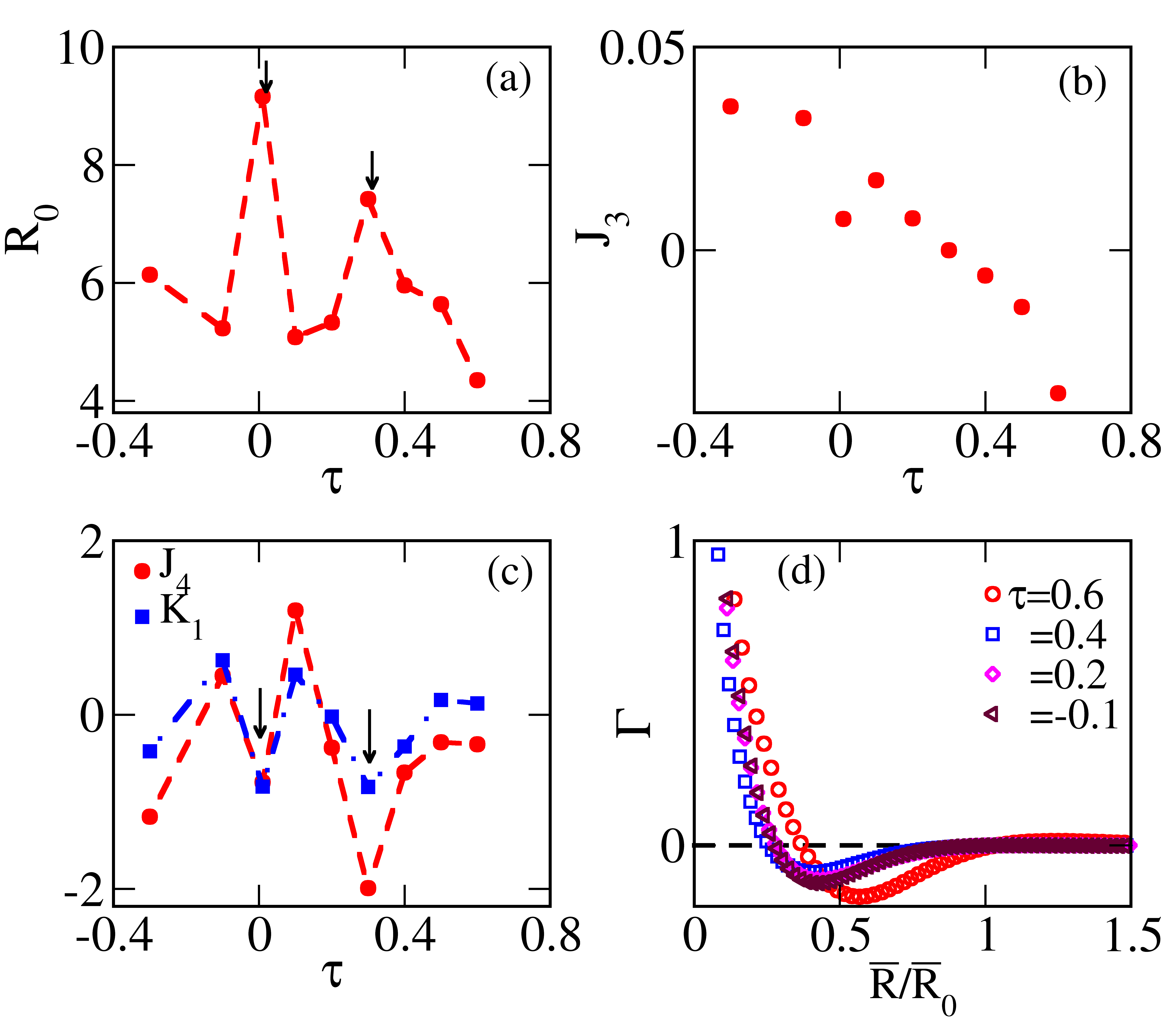
Refer to caption
Figure 15: (Color online) Signs of BG case curvature-dynamics coefficients: a) Plot of coefficient-evaluation choice R¯0(τ)subscript¯𝑅0𝜏{\bar{R}}_{0}(\tau) versus τ𝜏\tau from data, with dashed lines as guides to the eye. Arrows mark local maxima near τ=0𝜏0\tau=0 and τ=τf=0.3𝜏subscript𝜏𝑓0.3\tau=\tau_{f}=0.3. b) Plot of J30f¯0(T)/R¯0(τ)similar-tosubscript𝐽30subscript¯𝑓0𝑇subscript¯𝑅0𝜏J_{30}\sim{\bar{f}}_{0}(T)/{\bar{R}}_{0}(\tau) versus τ𝜏\tau, showing the change in sign at τf0.3similar-to-or-equalssubscript𝜏𝑓0.3\tau_{f}\simeq 0.3; c)Log-linear plot of (positive) coefficients log10(J40)subscript10subscript𝐽40\log_{10}(J_{40}), log10(K10)subscript10subscript𝐾10\log_{10}(K_{10}) versus τ𝜏\tau. Arrows mark local minima near τ=0,0.3𝜏00.3\tau=0,0.3. d) Plot of domain-wall correlation Γ(R¯)Γ¯𝑅\Gamma(\bar{R}) versus R¯/R¯0(τ)¯𝑅subscript¯𝑅0𝜏\bar{R}/{\bar{R}}_{0}(\tau), showing that it flattens to zero, close to our inflection-point choice of R¯/R¯0(τ)¯𝑅subscript¯𝑅0𝜏{\bar{R}}/{\bar{R}}_{0}(\tau).

An alternate choice of R¯¯𝑅\bar{R} for coefficient evaluation, is where the domain-wall correlations fall to zero. As domain walls carry nonzero OP gradients, we define the gradient-gradient OP correlations scaled in the curvature as

Γ(R¯)g2re(r,t).re(r,t)=g2r.rG(R¯)\Gamma(\bar{R})\equiv g^{-2}\langle\nabla_{\vec{r}}~{}e(\vec{r},t).\nabla_{\vec{r^{\prime}}}~{}e(\vec{r^{\prime}},t)\rangle=g^{-2}\nabla_{\vec{r}}.\nabla_{\vec{r^{\prime}}}G(\bar{R})
=D^G(R¯)=[G′′+(d1)G/R¯].(B2)formulae-sequenceabsent^𝐷𝐺¯𝑅delimited-[]superscript𝐺′′𝑑1superscript𝐺¯𝑅𝐵2=-{\hat{D}}G(\bar{R})=-[G^{\prime\prime}+(d-1)G^{\prime}/{\bar{R}}].~{}(B2)

This is a measure of DW correlations during coarsening, and also appears in the correlation dynamics of (5.9a), (5.9b). Fig 15d shows that Γ(R¯)Γ¯𝑅\Gamma(\bar{R}) flattens to zero close to R¯/R¯0=1¯𝑅subscript¯𝑅01{\bar{R}}/{{\bar{R}}_{0}}=1, so this alternative choice gives the same coefficient signs, as our G𝐺G-inflection choice.

Appendix C: Coarsening exponents

We here outline the procedure for numerically extracting, from curvature falloffs, the exponent values given in the text.

A possible diagnostic for whether g(t)𝑔𝑡g(t) has a powerlaw decay component 1/tαsimilar-toabsent1superscript𝑡𝛼\sim 1/t^{\alpha} is to plot tαg(t)superscript𝑡𝛼𝑔𝑡t^{\alpha}g(t) versus t𝑡t. It will flatten, where α𝛼\alpha is the most prominent contribution, and fall (or rise) as tαβsuperscript𝑡𝛼𝛽t^{\alpha-\beta}, where another exponent β𝛽\beta contributes more substantially. Fig 16a shows the variable

Yα=(tε¯4)α(g/ε¯2),(C1)subscript𝑌𝛼superscript𝑡superscript¯𝜀4𝛼𝑔superscript¯𝜀2𝐶1Y_{\alpha}=(t{\bar{\varepsilon}}^{4})^{\alpha}(g/{\bar{\varepsilon}}^{2}),~{}~{}~{}(C1)

plotted versus (tε¯4)𝑡superscript¯𝜀4(t{\bar{\varepsilon}}^{4}) for the test or trial values α=2/3,1/2𝛼2312\alpha=2/3,1/2. This shows clear signatures of single powerlaw decay contributions, with actual exponents close to these trial values. A supporting width-diagnostic for the time windows, is dlogg/dlogt𝑑𝑔𝑑𝑡d\log g/d\log t versus t𝑡t (not shown): although the data is noisy, it also shows flat regions as in Fig 16a. Fig 16b shows linear fits in log-log plots within these single-powerlaw, dominance windows, that yield the actual, numerically fitted exponents.
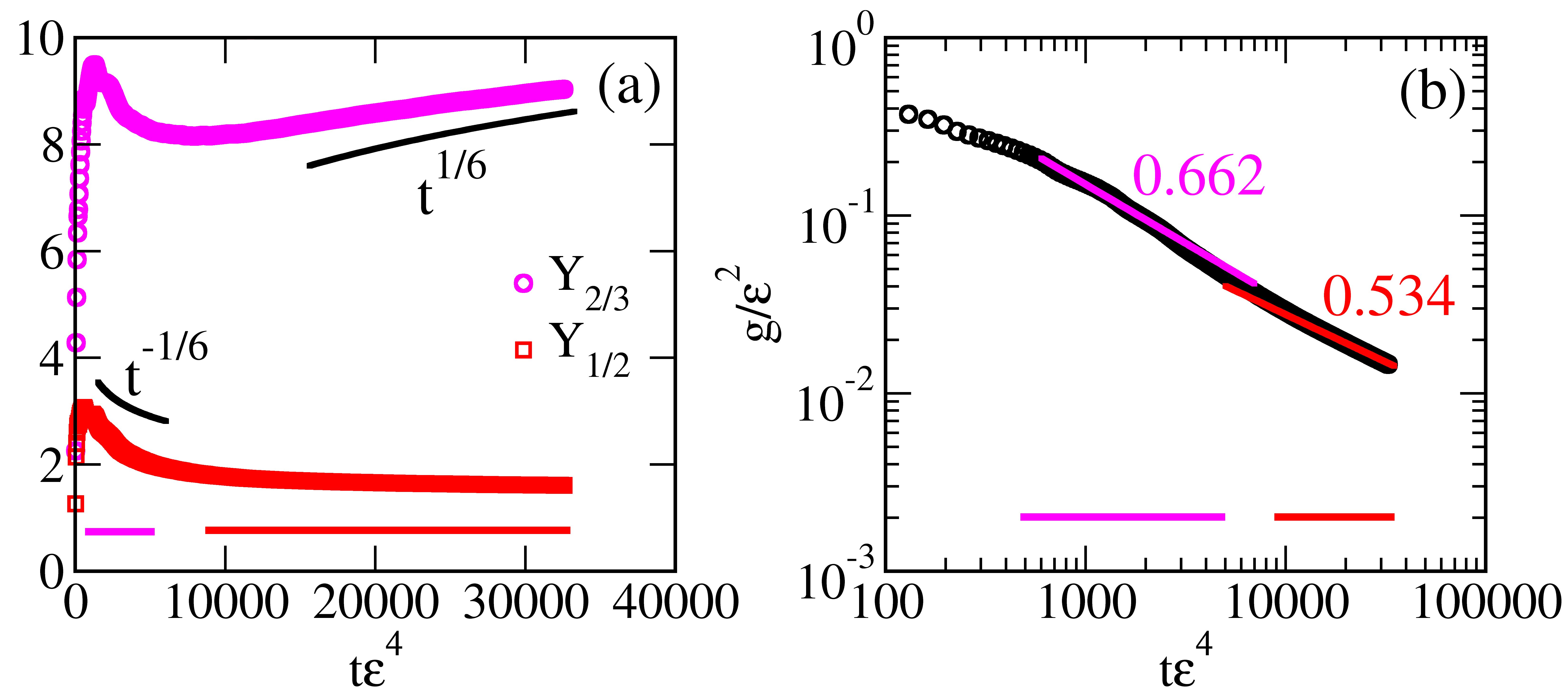
Refer to caption
Figure 16: (Color online) Intermediate and late time BG exponents for τ=0.2𝜏0.2\tau=0.2 : (a) Plot of data for Yαsubscript𝑌𝛼Y_{\alpha} defined in the text vs tε¯4𝑡superscript¯𝜀4t{\bar{\varepsilon}}^{4}, for test values α=2/3,1/2𝛼2312\alpha=2/3,1/2. Flat regions are from dominance of single power-laws, with exponents close to these test values. Horizontal bars denote the time windows taken, for numerical fits. (b) Plot of log10g/ε¯2subscript10𝑔superscript¯𝜀2\log_{10}g/{\bar{\varepsilon}}^{2} vs log10tε¯4subscript10𝑡superscript¯𝜀4\log_{10}t{\bar{\varepsilon}}^{4} showing lines numerically fitted, within the time windows (see text).

With this procedure, in the dominance time-windows, the exponent mean values and standard deviations, for τ=0.6,0.5,0.4,0.3,0.2,0.1,0.05𝜏0.60.50.40.30.20.10.05\tau=0.6,~{}0.5,~{}0.4,~{}0.3,~{}0.2,~{}0.1,~{}0.05 are found to be respectively α=0.619±0.012;0.680±0.018;0.688±0.014;0.683±;0.662±0.015;0.636±0.013;0.649±0.026𝛼plus-or-minus0.6190.012plus-or-minus0.6800.018plus-or-minus0.6880.014limit-from0.683plus-or-minusplus-or-minus0.6620.015plus-or-minus0.6360.013plus-or-minus0.6490.026\alpha=0.619\pm 0.012;~{}~{}0.680\pm 0.018;~{}~{}0.688\pm 0.014;~{}~{}0.683\pm;~{}~{}0.662\pm 0.015;~{}~{}0.636\pm 0.013;~{}~{}0.649\pm 0.026, which are all close to 2/3232/3. For τ=0.3,0.2,0.1,0.05𝜏0.30.20.10.05\tau=0.3,~{}0.2,~{}0.1,~{}0.05 the exponents are found to be α=0.555±0.03;0.534±0.02;0.543±0.01;0.497±0.01𝛼plus-or-minus0.5550.03plus-or-minus0.5340.02plus-or-minus0.5430.01plus-or-minus0.4970.01\alpha=0.555\pm 0.03;~{}~{}0.534\pm 0.02;~{}~{}0.543\pm 0.01;~{}~{}0.497\pm 0.01, which are all close to 1/2121/2. The exponents are expected to be τ𝜏\tau-independent, and a simple arithmetic average yields α=0.661±0.017;α=0.531±0.016formulae-sequence𝛼plus-or-minus0.6610.017𝛼plus-or-minus0.5310.016\alpha=0.661\pm 0.017;~{}~{}\alpha=0.531\pm 0.016. Keeping two significant figures for consistency,

α=0.66±0.02,and0.53±0.02.(C2)\alpha=0.66\pm 0.02,~{}~{}~{}{\text{a}nd}~{}~{}~{}0.53\pm 0.02.~{}~{}~{}~{}(C2)

For deep quenches of Fig 10, the other exponents seen are α=0.35±0.03;α=0.001±0.002formulae-sequence𝛼plus-or-minus0.350.03𝛼plus-or-minus0.0010.002\alpha=0.35\pm 0.03;~{}~{}\alpha=0.001\pm 0.002, which are close to 1/3131/3 and 00. See Sec. VI on coarsening arrest.

References

  • (1) A.J. Bray, Advances in Physics, 51, 481 (2002).
  • (2) Kinetics of Phase Transitions, edited by S. Puri and V. Wadhawan, (CRC Press, Florida (2009)).
  • (3) K.  Bhattacharya, Microstructure of Martensite, (Oxford University Press, Oxford, 2003);.
  • (4) J. W. Cahn and J. E. Hilliard, J. Chem. Phys 28, 258 (1958); S. Puri, in Ref. [2].
  • (5) J. S. Langer, M. Bar-on and H.D. Miller, Phys. Rev. A 11, 1417 (1975).
  • (6) E.D. Siggia, Phys. Rev. A 20, 595 (1979); A.J. Bray and E. Rutenberg, Phys. Rev. E, 49, R27 (1994).
  • (7) A.J. Bray and S. Puri, Phys. Rev. Lett. 67, 2670 (1991).
  • (8) Y. Oono and S. Puri, Phys. Rev. Lett. 58, 836 (1987); Phys. Rev. A 38, 434 (1988);
    S. Puri and Y. Oono, Phys. Rev. A 38, 1542 (1988).
  • (9) CH exponents α=1/4,1/3𝛼1413\alpha=1/4,1/3 have been found. S. Puri, A.J. Bray and J.L. Lebowitz, Phys. Rev. E 56, 758 (1997); S. van Gemmert, G.T. Barkema and S. Puri, Phys. Rev. E 72, 046131 (2005); G. Sheng, T. Wang, Q. Du, K.G. Wang, Z. K. Liu, and L. Q. Chen, Commun. Comput. Phys., 8, 249 (2010). Continuum-strain evolutions e(r,t)𝑒𝑟𝑡e(\vec{r},t) involve both a slow re-arrangement of domain walls, and a faster relaxation of strains on either side of the DW to their final, equilibrium values ±ε¯plus-or-minus¯𝜀\pm{\bar{\varepsilon}}. To reduce noisy data from the latter, one can promptly set the strain, to the equilibrium value it will attain, once the sign is determined by the evolution dynamics, in a ’strain hardening’ procedure, that focuses on the relevant slower DW timescales, for structure factors.
  • (10) A. Singh, S. Puri and H. Mishra, Nucl. Phys. A 864, 176 (2011); Nucl. Phys. A 908, 12 (2013).
  • (11) M. San Miguel, M. Grant and J.D. Gunton, Phys. Rev. A 31, 1001 (1985); T. Ohta, D. Jasnow and K. Kawasaki, Phys. Rev. Lett. 49, 1223 (1982); G. F. Mazenko, Phys. Rev. Lett. 63, 1605 (1989); Phys. Rev. B 42, 4487 (1990). Phys. Rev. B 43, 5747 (1991).
  • (12) B. Sciolla and G. Biroli, Phys. Rev. B 88, 201110(R), (2013).
  • (13) P.C. Hohenberg and B. I. Halperin, Rev. Mod. Phys. 49, 435 (1977); Phys. Rev. 177,952 (1969).
  • (14) G.R. Barsch and J.A. Krumhansl Phys. Rev. Lett. 53, 1069 (1984).
  • (15) S. Kartha, J.A. Krumhansl, J.P. Sethna, and L. K. Wickham, Phys. Rev. B 52, 803 (1995).
  • (16) S.R. Shenoy, T. Lookman, A. Saxena, and A. R. Bishop, Phys. Rev. B 60, R12537 (1999).
  • (17) S.R. Shenoy, T. Lookman and A. Saxena, Phys. Rev. B 82, 144103 (2010).
  • (18) N. Shankaraiah, K.P.N. Murthy, T. Lookman and S.R. Shenoy, Europhys. Lett. 92, 36002 (2010); Phys. Rev. B 84, 064119 (2011); Phys. Rev. B 91, 214108 (2015).
  • (19) G.S. Bales and R.J. Gooding, Phys. Rev. Lett. 67, 3412 (1991).
  • (20) T. Lookman, S.R. Shenoy, K.O. Rasmussen, A. Saxena and A.R. Bishop, Phys. Rev. B 67 024114 (2003).
  • (21) A. Paul, J. Bhattacharya, S. Sengupta and M. Rao, J. Phys: Condens. Matt. 20. 365211 (2008); A. Onuki, J. Phys. Soc. Jpn. 68, 5 (1999).
  • (22) Y. Gao, J. Kim and M.E. Helgeson, Soft Matter 11, 6360 (2015); P. Perlekar, R. Benzi, H.J. H. Clerex, D.R. Nelson and F. Toschi, Phys. Rev. Lett. 112, 014502 (2014); P. Perlekar, N. Pal and R. Pandit, arXiv:1506.08524v1 physics.fl-dyn.
  • (23) The evolutions from random dilute seeds in a zero-OP background depend on both the temperature and the seed size, as is reasonable for a first-order transition with a critical droplet radius for expansion. A surrogate-droplet parametrization of complex-texture energies was introduced in a discretized-strain Monte Carlo context R18 , with the Hamiltonian energy H(t)𝐻𝑡H(t) taken as proportional to simple energy expression of a surface plus bulk energy in 2D as fL(T)R(t)2+R(t)subscript𝑓𝐿𝑇𝑅superscript𝑡2𝑅𝑡f_{L}(T)R(t)^{2}+R(t). For t=0𝑡0t=0 (only), the energy parameter R(t)𝑅𝑡R(t) has the geometric meaning of an initial seed size R(0)𝑅0R(0). There is a critical parameter Rc(T)subscript𝑅𝑐𝑇R_{c}(T) that for A1=0subscript𝐴10A_{1}=0 is defined as Rc2ξ02ε¯2/|fL(τ)|subscript𝑅𝑐2superscriptsubscript𝜉02superscript¯𝜀2subscript𝑓𝐿𝜏R_{c}\equiv 2\xi_{0}^{2}{\bar{\varepsilon}}^{2}/|f_{L}(\tau)|, that diverges at τ=1𝜏1\tau=1. The surrogate-droplet energy versus R(0)/Rc(T)𝑅0subscript𝑅𝑐𝑇R(0)/R_{c}(T), is a single inverted parabola for all temperatures. Our continuous-strain dynamics simulations also fall on such a curve, as a bench-mark.
  • (24) We multiply the dynamics for e(r,t)𝑒𝑟𝑡e({\vec{r}},t) by e(r,t)𝑒superscript𝑟superscript𝑡e(\vec{r^{\prime}},t^{\prime}) and set r=R+r0𝑟𝑅subscript𝑟0\vec{r}=\vec{R}+\vec{r}_{0}, r=r0superscript𝑟subscript𝑟0\vec{r^{\prime}}=\vec{r}_{0}, to get an equation for C(R,t,t)𝐶𝑅𝑡superscript𝑡C(\vec{R},t,t^{\prime}) where R=rr𝑅𝑟superscript𝑟\vec{R}=\vec{r}-\vec{r^{\prime}}. We then take a dynamics for e(r,t)𝑒superscript𝑟superscript𝑡e(\vec{r^{\prime}},t^{\prime}) and multiply by e(r,t)𝑒𝑟𝑡e({\vec{r}},t), set r=r0𝑟subscript𝑟0\vec{r}=\vec{r}_{0}, r=R+r0superscript𝑟𝑅subscript𝑟0\vec{r^{\prime}}=-\vec{R}+\vec{r}_{0}, to get an equation for C(R,t,t)𝐶𝑅𝑡superscript𝑡C(-\vec{R},t,t^{\prime}). Adding, and letting ttsuperscript𝑡𝑡t^{\prime}\rightarrow t, we get a dynamics for the symmetrized OP-OP correlation Csym(R,t)=12[C(R,t)+C(R,t)]subscript𝐶𝑠𝑦𝑚𝑅𝑡12delimited-[]𝐶𝑅𝑡𝐶𝑅𝑡C_{sym}(\vec{R},t)=\frac{1}{2}[C(\vec{R},t)+C(-\vec{R},t)] in terms of the symmetrized μ𝜇\mu-OP correlation Csym(μ)=12[C(μ)(R,t)+C(μ)(R,t)]superscriptsubscript𝐶𝑠𝑦𝑚𝜇12delimited-[]superscript𝐶𝜇𝑅𝑡superscript𝐶𝜇𝑅𝑡{C_{sym}}^{(\mu)}=\frac{1}{2}[C^{(\mu)}(\vec{R},t)+C^{(\mu)}(-\vec{R},t)], whose Fourier transform thus depends only on the real part Csym(μ)(k)Re[μ(k,t)e(k,t)]similar-tosuperscriptsubscript𝐶𝑠𝑦𝑚𝜇𝑘𝑅𝑒delimited-[]𝜇𝑘𝑡𝑒superscript𝑘𝑡{C_{sym}}^{(\mu)}(\vec{k})\sim Re[\mu(\vec{k},t){e(\vec{k},t)}^{\ast}], and we drop the subscript. On angular averaging, the correlation depends on |k|𝑘|\vec{k}| only.
  • (25) From the unscaled curvature kinetics of (6.2), in the damping regime, a powerlaw falloff g(K10/J40)1/2/t1/2similar-to-or-equals𝑔superscriptsubscript𝐾10subscript𝐽4012superscript𝑡12g\simeq(K_{10}/J_{40})^{1/2}/t^{1/2} could crossover to an even smaller tail g(K10/J30)/t<<1similar-to-or-equals𝑔subscript𝐾10subscript𝐽30𝑡much-less-than1g\simeq(K_{10}/J_{30})/t<<1, at very long times 105similar-toabsentsuperscript105\sim 10^{5}, much larger than the present holding time th=20,000subscript𝑡20000t_{h}=20,000.
  • (26) In Monte Carlo simulations R18 , (with compatibilty interactions), there are transient zeros of the OP acting as dynamical catalysts, that facilitate domain wall rearrangements. For τ𝜏\tau well below the Landau spinodal, nucleation of these catalysts became less probable, and domain walls can form a glassy state, with trapped internal stresses. In the present OP dynamics simulation, a similar glass-like trapping seems to occur, for sub-spinodal quench temperatures.