Weighted Matrix Completion and Recovery
with Prior Subspace Information

Abstract

An incoherent low-rank matrix can be efficiently reconstructed after observing a few of its entries at random, and then solving a convex program that minimizes the nuclear norm. In many applications, in addition to these entries, potentially valuable prior knowledge about the column and row spaces of the matrix is also available to the practitioner. In this paper, we incorporate this prior knowledge in matrix completion—by minimizing a weighted nuclear norm—and precisely quantify any improvements. In particular, we find in theory that reliable prior knowledge reduces the sample complexity of matrix completion by a logarithmic factor, and the observed improvement in numerical simulations is considerably more magnified. We also present similar results for the closely related problem of matrix recovery from generic linear measurements.

I Introduction

Matrix completion is commonly defined as the problem of recovering a low-rank matrix $M\in\mathbb{R}^{n\times n}$ from a fraction of its entries, observed on an often random index set [1, 2]. More concretely, let $r$ denote the rank of $M$. Also let $M=U_{r}\Sigma_{r}V_{r}^{*}$ be a (thin) singular value decomposition (SVD) of $M$, where $U_{r},V_{r}\in\mathbb{R}^{n\times r}$ have orthonormal columns and the diagonal matrix $\Sigma_{r}\in\mathbb{R}^{r\times r}$ contains the singular values of $M$.

In a typical low-rank matrix completion problem, each entry of $M$ is observed with a probability of $p\in(0,1]$ so that $pn^{2}$ entries of $M$ are revealed in expectation. Let the matrix $Y=\mathcal{R}_{p}(M)\in\mathbb{R}^{n\times n}$ contain the observed entries of $M$ with zeros everywhere else. Here, $\mathcal{R}_{p}(\cdot)$ represents the measurement process. In fact, with overwhelming probability, $M$ can be successfully reconstructed from the measurements $Y$ by solving the convex program

$$\begin{cases}\min_{X}\left\|X\right\|_{*},\\ \mbox{subject to }\mathcal{R}_{p}(X)=Y,\end{cases}$$ (1)

provided that

$$1\geq p\gtrsim\frac{\eta(M)r\log^{2}n}{n}.$$ (2)

Above, the nuclear norm $\|X\|_{*}$ returns the sum of singular values of a matrix $X$. In addition, the coherence $\eta(M)$ measures how “spiky” $M$ is, as precisely defined later in Section II. One can therefore expect to successfully recover $M$ from $O(\eta(M)\cdot rn\log^{2}n)$ uniform samples [3, 4, 5].

I-A Incorporating Prior Knowledge

Let $\operatorname{U}_{r}=\mbox{span}(U_{r})$ and $\operatorname{V}_{r}=\mbox{span}(V_{r})$ be the column and row spaces of $M=U_{r}\Sigma_{r}V_{r}^{*}$. Suppose that we have been presented with some prior knowledge about $M$ in the form of estimates for the subspaces $\operatorname{U}_{r}$ and $\operatorname{V}_{r}$. More specifically, let the $r$-dimensional subspaces $\widetilde{\operatorname{U}}_{r}$ and $\widetilde{\operatorname{V}}_{r}$ be the initial estimates of the column and row spaces of $M$, respectively, made available to us.

As an example in the context of collaborative filtering, $\widetilde{\operatorname{U}}_{r}$ might represent the similarities among users in the “Netflix challenge”. To be specific, the rows and columns of the popular Netflix matrix correspond to the Netflix subscribers and available movies, respectively. The Netflix matrix is sparsely populated with the ratings assigned by its users and the challenge is then to complete the Netflix matrix given only the ratings available, namely given only a small fraction of its entries. A more realistic setup for the Netflix challenge should perhaps incorporate the changes in the preferences of Netflix users over time which are for example significantly altered by child-rearing, see [6] for such temporal dynamics. Here, $\widetilde{\operatorname{U}}_{r}$ might incorporate prior information about the users and for instance might be obtained by taking an SVD of the current estimate of the database matrix $M$, with the anticipation that these features and thus $M$ itself might change over time. Similar problems arise in tracking changes in videos or updating the Laplacian of a graph with time-variant connectivity. See [7, 8] for more examples.

As another example, in exploration seismology, large and often incomplete matrices are acquired and processed in order to determine the subsurface structure of an area. Each target matrix is comprised of responses from many sources at a certain frequency recorded at many receivers, where some recordings are missing. In this context, information from adjacent frequency bands might help enhance completion of the target matrix. More specifically, one might set $\widetilde{\operatorname{U}}_{r}$ to be the column space of the estimated response matrix from an adjacent frequency band and perform the reconstruction band-by-band in a “dynamic” fashion similar to the collaborative filtering setup above, see [9, Sec. 8] for full details. The resulting algorithm would iteratively update the estimate of $t$th slice of the data tensor based on the estimate from, say, the $t-1$th slice, and cycle through the tensor multiple times if needed. These ideas might also be generalized to the problem of subspace tracking from incomplete data, in which we are interested in recovering a subspace from a sequence of generic vectors in that subspace, observed partially. This subspace tracking problem is also closely related to streaming principal component analysis [10, 11]. The related literature is more carefully studied later in Section V.

Motivated by such scenarios, it is perhaps natural to ask:

• Question: How should we incorporate in matrix completion any prior knowledge about column and row spaces?

We approach this question with the aid of a weighted nuclear norm as follows. Let $P_{\widetilde{\operatorname{U}}_{r}},P_{\widetilde{\operatorname{U}}_{r}^{\perp}}\in\mathbb{R}^{n\times n}$ be the orthogonal projections onto the subspace $\widetilde{\operatorname{U}}_{r}$ and its orthogonal complement $\widetilde{\operatorname{U}}_{r}^{\perp}$, respectively. For some weight $w\in(0,1]$, define

$$Q_{\widetilde{\operatorname{U}}_{r},w}:=w\cdot P_{\widetilde{\operatorname{U}}_{r}}+P_{\widetilde{\operatorname{U}}_{r}^{\perp}}\in\mathbb{R}^{n\times n}.$$ (3)

Likewise, define ${\color[rgb]{0,0,0}Q_{\widetilde{\operatorname{V}}_{r},w}}\in\mathbb{R}^{n\times n}$ and let us modify Program (1) to read

$$\begin{cases}\min_{X}\left\|{\color[rgb]{0,0,0}Q_{\widetilde{\operatorname{U}}_{r},w}\cdot X\cdot Q_{\widetilde{\operatorname{V}}_{r},w}}\right\|_{*},\\ \mbox{subject to }\mathcal{R}_{p}(X)=Y.\end{cases}$$ (4)

In a sense, the weight $w$ reflects our uncertainty in the prior knowledge. The smaller $w$, the more confident we are that $\operatorname{U}_{r}\approx\widetilde{\operatorname{U}}_{r}$ and $\operatorname{V}_{r}\approx\widetilde{\operatorname{V}}_{r}$ and in turn the more penalty Program (4) places on feasible matrices with column or row spaces orthogonal to $\widetilde{\operatorname{U}}_{r}$ or $\widetilde{\operatorname{V}}_{r}$, respectively. In contrast, when our prior information is not reliable, we might set $w=1$, in which case $Q_{\widetilde{\operatorname{U}}_{r},w}=Q_{\widetilde{\operatorname{V}}_{r},w}=I_{n}$ and Program (4) reduces to standard matrix completion, namely Program (1), thereby completely ignoring any prior knowledge about the problem.

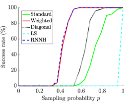
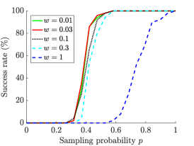
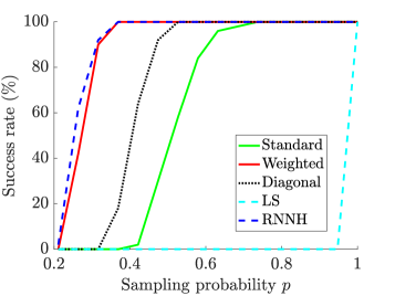
A more general form of Program (4) is discussed in Section II in greater detail. For now, let us briefly compare the two Programs (1) and (4) in practice. We take $M$ be a square matrix of sidelength $n=20$, rank $r=4$, and norm $\|M\|_{F}=1$. As prior knowledge to be used in completing $M$, we construct a perturbed version $M^{\prime}$ of $M$, where $M^{\prime}=M+N$ and entries of $N\in\mathbb{R}^{n\times n}$ are independent Gaussian random variables with mean zero and variance $10^{-4}$. We then compute the SVD of $M^{\prime}$ and let $(\widetilde{\operatorname{U}}_{r},\widetilde{\operatorname{V}}_{r})$ contain the leading $r$ left- and right-singular vectors of $M^{\prime}$. Lastly we set the weight $w=0.1$. As the probability $p$ of observing each entry of $M$ varies in $(0,1]$, we solve both Programs (1,4) and record the results. The success rates for both programs, averaged over $50$ trials, is shown in Figure 1a. (Program (1) corresponds to the solid green line, Program (4) corresponds to the solid red line, and other lines are explained in Section IV.) A trial is considered successful if it recovers $M$ up to a relative error of $10^{-3}$. Observe how reliable prior knowledge, when used properly, allows for successful matrix completion from substantially fewer measurements.

(a)

(b)

(c)

Figure 1: Matrix completion with prior information, where the principal angles between the ground truth and prior knowledge subspaces are $u=\angle[\operatorname{U}_{r},{\widetilde{\operatorname{U}}}_{r}]=0.099$ and $v=\angle[\operatorname{V}_{r},\widetilde{\operatorname{V}}_{r}]=0.103$. (a) compares standard matrix completion via Program (1), weighted matrix completion proposed in Program (4) with $w=0.1$, diagonal weighted matrix completion, weighted least-squares, and a weighted nuclear norm heuristic (RNNH) algorithm with the tuning parameter $\delta=0.01$. (b) shows the performance of weighted matrix completion with various weights $w$. (c) shows RNNH with various parameters $\delta$. See Section IV for more details.

I-B Simplified Main Result

One of our main results in this paper concerns the performance of a more general form of Program (4), which we next outline, deferring a more rigorous statement of the result to Theorem 2 in Section III.

Consider a rank-$r$ matrix $M\in\mathbb{R}^{n\times n}$, and let $\operatorname{U}_{r}=\mbox{span}(M)$ and $\operatorname{V}_{r}=\mbox{span}(M^{*})$ be the column and row spaces of $M$. Let also $\eta(M)$ be the coherence of $M$, which we briefly introduced earlier.

Suppose also that the $r$-dimensional subspaces ${\widetilde{\operatorname{U}}}_{r}$ and $\widetilde{\operatorname{V}}_{r}$, with orthonormal bases $\widetilde{U}_{r},\widetilde{V}_{r}\in\mathbb{R}^{n\times r}$, represent our prior knowledge about the column and row spaces of $M$, respectively. In particular, let $u=\angle[\operatorname{U}_{r},{\widetilde{\operatorname{U}}}_{r}]$ and $v=\angle[\operatorname{V}_{r},\widetilde{\operatorname{V}}_{r}]$ denote the largest principal angles between each pair of subspaces. We set $\theta=\max[u,v]$ for short. Moreover, consider the sampling probability $p\in(0,1]$ and let $Y=\mathcal{R}_{p}(M)$ be the matrix of measurements, defined earlier. Lastly, for weight $w\in(0,1]$, let $\widehat{M}$ be a solution of Program (4). Then, $\widehat{M}=M$, except with a probability of $o(n^{-19})$ and provided that

$$1\geq p\gtrsim\max\left[\log\left(\Cl[factors]{4p}\cdot n\right),1\right]\cdot\frac{\eta(M)r\log n}{n}$$

$$\qquad\qquad\qquad\qquad\,\cdot\mbox{inter-coherence factor},$$

$$\Cl[factors]{3p}\leq\frac{1}{8},$$ (5)

where the “inter-coherence factor” above, to be made precise later, is often not large and reflects the interaction between the coherence of prior subspaces and the true ones. Additionally,

$$\Cr{4p}:={\frac{w^{4}\cos^{2}\theta+\sin^{2}\theta}{w^{2}\cos^{2}\theta+\sin^{2}\theta}},\quad\Cr{3p}:=\frac{3\sqrt{1-w^{2}}\sin\theta}{\sqrt{w^{2}\cos^{2}\theta+\sin^{2}\theta}}.$$

In particular, when $w=1$, then the prior information $(\widetilde{\operatorname{U}}_{r},\widetilde{\operatorname{V}}_{r})$ is ignored and Program (4) reduces to Program (1). In this case, $\Cr{4p}=1,\Cr{3p}=0$ and (5) reduces to (2), save for the typically small coherence factor.

On the other hand, when our prior knowledge is reliable, namely when $\theta$ is small, the proper choice of $w$ in Program (4) leads to substantial improvement over Program (1). For example, with $\sin\theta\lesssim 1/n$ and $w=\sqrt{\tan\theta}$, observe that $\Cr{4p}=O(\sin\theta)$, $\max\left[\log\left(\Cr{4p}\cdot n\right),1\right]=1$, $\Cr{3p}=O(\sqrt{\sin\theta})$, and (5) now reads as

$$1\geq p\gtrsim\frac{\eta(M)r\log n}{n},$$ (6)

save for the often small inter-coherence factor. The lower bound in (6) is better than (2) by a logarithmic factor and is likely near optimal, as discussed in Section III.

I-C Matrix Recovery with Prior Knowledge

Matrix completion, discussed above, is a special case of the more general matrix recovery problem, in which the objective is to recover a matrix from generic and often random linear measurements. This problem is reviewed in Section II and our other main result, Theorem 1 in Section III, concerns leveraging prior information in this context.

I-D Organization

The rest of this paper is organized as follows. In Section II, we briefly review standard low-rank matrix recovery and completion, and further motivate the use of prior knowledge in these contexts. Our main results quantify the use of prior knowledge in matrix recovery and completion, and are summarized in Section III. Section IV offers some numerical evidence to support the theory and the related literature is highlighted in Section V. Technical details are postponed to Sections VI-VIII and appendices. In particular, Section VI collects the technical tools common to the analysis of both matrix recovery and completion. Sections VII and VIII then contain the arguments specialized to matrix recovery and completion, respectively.

II Problem Statement

Consider a matrix $M\in\mathbb{R}^{n\times n}$ and its SVD $M=U\Sigma V^{*}$. Here, $U,V\in\mathbb{R}^{n\times n}$ are orthonormal bases and the diagonal matrix $\Sigma\in\mathbb{R}^{n\times n}$ collects the singular values of $M$ in a non-increasing order, namely $\sigma_{1}(M)\geq\sigma_{2}(M)\geq\cdots\geq\sigma_{n}(M)$. For an integer $r\leq n$, let $U_{r},V_{r}\in\mathbb{R}^{n\times r}$ comprise of the first $r$ columns of $U,V$, respectively and let $\Sigma_{r}\in\mathbb{R}^{r\times r}$ contain $r$ largest singular values of $M$. Ties are broken arbitrarily. Then, $M_{r}=U_{r}\Sigma_{r}V_{r}^{*}\in\mathbb{R}^{n\times n}$ is a rank-$r$ truncation of $M$ and we also let $M_{r^{+}}=M-M_{r}$ denote the residual.

Suppose that we can only access $M\in\mathbb{R}^{n\times n}$ through a linear operator $\mathcal{R}_{m}(\cdot)$ that collects $m$ measurements from $M$. More specifically, let

$$y=\mathcal{R}_{m}(M+E)\in\mathbb{R}^{m},\qquad\left\|\mathcal{R}_{m}(E)\right\|_{2}\leq e,$$ (7)

be the vector of $m$ (possibly noisy) measurements. Here, $E\in\mathbb{R}^{n\times n}$ and $e\geq 0$ represent the noise. Matrix recovery is then the problem of (approximately) reconstructing $M$ from the measurement vector $y$.

The case where the entries of $M$ are randomly observed is of particular importance in practice, where we pragmatically assume that a measurement operator $\mathcal{R}_{p}(\cdot)$ observes each entry of $M$ with a probability of $p\in(0,1]$. We set $p=m/n^{2}$ so that $\mathcal{R}_{p}(M)$ contains $m$ entries of $M$, in expectation. To be more specific, $\mathcal{R}_{p}(\cdot)$ takes $M\in\mathbb{R}^{n\times n}$ to $\mathcal{R}_{p}(M)\in\mathbb{R}^{n\times n}$ defined as

$$\mathcal{R}_{p}(M)=\sum_{i,j=1}^{n}\frac{\epsilon_{ij}}{p}\cdot M[i,j]\cdot C_{ij},$$ (8)

where $\{\epsilon_{ij}\}_{i,j}$ is a sequence of independent Bernoulli random variables taking one with probability of $p$ and zero otherwise. Throughout, $C_{ij}\in\mathbb{R}^{n\times n}$ is the $[i,j]$th canonical matrix, so that $C_{ij}[i,j]=1$ is its only nonzero entry. We also let

$$Y=\mathcal{R}_{p}(M+E)\in\mathbb{R}^{n\times n},\qquad\left\|\mathcal{R}_{p}(E)\right\|_{F}\leq e,$$ (9)

be the (possibly noisy) matrix of measurements. As before, $E$ and $e$ represent the noise. Matrix completion is the problem of (approximately) reconstructing $M$ from $Y$.

II-A Standard Low-Rank Matrix Recovery and Completion

In general, both matrix recovery and completion problems are ill-posed when $m\leq n^{2}$ and, to rectify this issue, it is common to impose that $M$ is (nearly) low-rank. Let us briefly review both low-rank matrix completion and recovery next.

In low-rank matrix recovery, the restricted isometry property (RIP) plays a key role by ensuring that the measurement operator preserves the geometry of the set of low-rank matrices. More specifically, for $\delta_{r}\in[0,1)$, we say that $\mathcal{R}_{m}(\cdot)$ satisfies the $(r,\delta_{r})$-RIP (or simply $\delta_{r}$-RIP when there is no ambiguity) if

$$\left(1-\delta_{r}\right)\|X\|_{F}\leq\left\|\mathcal{R}_{m}(X)\right\|_{2}\leq\left(1+\delta_{r}\right)\|X\|_{F},$$

for every $X\in\mathbb{R}^{n\times n}$ with $\mbox{rank}(X)\leq r$. It is perhaps remarkable that a “generic” linear operator from $\mathbb{R}^{n\times n}$ to $\mathbb{R}^{m}$ satisfies the RIP when the number of measurements $m$ is sufficiently large. For example, suppose that $G\in\mathbb{R}^{n\times n}$ is populated with independent zero-mean Gaussian random variables with variance $1/m$. Then, $\langle G,X\rangle$ collects one linear measurement from $X$. The measurement operator formed from $m$ independent copies of $\langle G,X\rangle$ is known to satisfy $\delta_{r}$-RIP with high probability when $m\gtrsim rn\log n/\delta_{r}^{2}$. When $M$ is nearly low-rank (in the sense that the residual $M_{r^{+}}=M-M_{r}$ is small) and when $\mathcal{R}_{m}(\cdot)$ satisfies the RIP, we can in fact (approximately) recover $M$ by solving the following convex program:

$$\begin{cases}\min_{X}\left\|X\right\|_{*},\\ \mbox{subject to }\left\|\mathcal{R}_{m}(X)-y\right\|_{2}\leq e.\end{cases}$$ (11)

Above, with $\{\sigma_{i}(X)\}_{i}$ standing for the singular values of the matrix $X$, $\|X\|_{*}=\sum_{i}\sigma_{i}(X)$ is the nuclear norm of $X$. We also use the Frobenius norm $\|X\|_{F}=(\sum_{i}\sigma_{i}^{2}(X))^{\frac{1}{2}}$ below. The recovery error of Program (11) is summarized next [12, 13].

Proposition 1.

(Matrix recovery) For an integer $r\leq n$ and matrix $M\in\mathbb{R}^{n\times n}$, let $M_{r}\in\mathbb{R}^{n\times n}$ be a rank-$r$ truncation of $M$ and let $M_{r^{+}}=M-M_{r}$ be the residual. Suppose that the linear measurement operator $\mathcal{R}_{m}:\mathbb{R}^{n\times n}\rightarrow\mathbb{R}^{m}$ satisfies $\delta_{5r}$-RIP with $\delta_{5r}\leq 0.1$. Let also $\widehat{M}\in\mathbb{R}^{n\times n}$ be a solution of Program (11). Then it holds that

$$\left\|\widehat{M}-M\right\|_{F}\lesssim\frac{\left\|M_{r^{+}}\right\|_{*}}{\sqrt{r}}+e.$$ (12)

In low-rank matrix completion, on the other hand, $\mathcal{R}_{p}(\cdot)$ does not satisfy the RIP unless $p\approx 1$, in which case nearly every entry of $M$ is observed anyway. For example, with $C_{11}$ standing for the first canonical matrix in $\mathbb{R}^{n\times n}$, note that $\mathcal{R}_{p}(C_{11})=0$ with a probability of $1-p$ and so $p$ must be close to one to capture the energy of $C_{11}$. However, $\mathcal{R}_{p}(\cdot)$ does preserve the geometry of the set of low-rank and incoherent matrices, provided that $p$ is sufficiently large. More specifically, let $M_{r}=U_{r}\Sigma_{r}V_{r}^{*}$ be an SVD of $M_{r}$, a rank-$r$ truncation of $M$. Then the coherence of $M_{r}$, denoted by $\eta(M_{r})$ throughout, is defined as

$$\eta\left(M_{r}\right)=\frac{n}{r}\max\left[\left\|U_{r}\right\|^{2}_{2\rightarrow\infty},\left\|V_{r}\right\|^{2}_{2\rightarrow\infty}\right],$$ (13)

where $\|X\|_{2\rightarrow\infty}$ returns the largest $\ell_{2}$ norm of the rows of $X$. It is not difficult to verify that $\eta(M_{r})\in[1,\frac{n}{r}]$, and that $\eta(M_{r})$ depends only on the column and row spaces of $M_{r}$. When $\eta(M_{r})$ is small, entries of $M_{r}$ tend to be roughly equal in magnitude and we say that $M_{r}$ is incoherent. At the other extreme, when $\eta(M_{r})$ is large, $M_{r}$ is often “spiky” and we say that $M_{r}$ is coherent. When $M$ is nearly low-rank and incoherent, we can (approximately) reconstruct $M$ by solving the convex program

$$\begin{cases}\min_{X}\left\|X\right\|_{*},\\ \mbox{subject to }\left\|\mathcal{R}_{p}(X)-Y\right\|_{F}\leq e,\end{cases}$$ (14)

for which the recovery error is obtained by slightly modifying Theorem 7 in [3] to fit our setup [14, Proposition 2].

Proposition 2.

(Matrix completion) For an integer $r\leq n$ and matrix $M\in\mathbb{R}^{n\times n}$, let $M_{r}\in\mathbb{R}^{n\times n}$ be a rank-$r$ truncation of $M$ and let $M_{r^{+}}=M-M_{r}$ be the residual. Let $\widehat{M}\in\mathbb{R}^{n\times n}$ be a solution of Program (14). Then, except with a probability of at most $o(n^{-19})$, it holds that

$$\left\|\widehat{M}-M\right\|_{F}\lesssim\frac{\left\|M_{r^{+}}\right\|_{*}}{\sqrt{p}}+e\sqrt{pn},$$ (15)

provided that

$$1\geq p\gtrsim\frac{\eta\left(M_{r}\right)r\log^{2}n}{n}.$$ (16)

For instance, when $M_{r}$ is incoherent, say $\eta_{r}(M_{r})\approx 1$, solving Program (14) approximately completes $M$ after observing only $O(rn\log^{2}n)$ of its samples, in expectation.

II-B Incorporating Prior Knowledge

Ideally, if the column and row spaces of a rank-$r$ matrix $M_{r}$ were known a priori, only $r^{2}$ linear measurements of $M_{r}$ would suffice for exact recovery in the absence of noise. Indeed, if rank-$r$ matrices $A_{r},B_{r}\in\mathbb{R}^{n\times r}$ span the column and row spaces of $M_{r}$, then $A_{r}^{*}M_{r}B_{r}\in\mathbb{R}^{r\times r}$ contains all the necessary information to reconstruct $M_{r}$.

More generally, consider $M\in\mathbb{R}^{n\times n}$ and let $M_{r}$ be a rank-$r$ truncation of $M$ as before. If available, suppose that the $r$-dimensional subspaces $\widetilde{\operatorname{U}}_{r}$ and $\widetilde{\operatorname{V}}_{r}$ represent our prior knowledge about the column and row spaces of $M_{r}=U_{r}\Sigma_{r}V_{r}^{*}$. In order to incorporate this prior knowledge into matrix recovery and completion, we propose the following approach. Let

$$P_{{\widetilde{\operatorname{U}}}_{r}}\in\mathbb{R}^{n\times n}\mbox{ and }P_{{\widetilde{\operatorname{U}}}_{r}^{\perp}}\in\mathbb{R}^{n\times n}$$

be the orthogonal projections onto the subspace $\widetilde{\operatorname{U}}_{r}$ and its complement, respectively. Likewise, we define $n\times n$ projection matrices $P_{\widetilde{\operatorname{V}}_{r}}$ and $P_{\widetilde{\operatorname{V}}_{r}^{\perp}}$. For (left and right) weights $\lambda,\rho\in[0,1]$, set

$$Q_{{\widetilde{\operatorname{U}}}_{r},\lambda}:=\lambda\cdot P_{{\widetilde{\operatorname{U}}}_{r}}+P_{{\widetilde{\operatorname{U}}}_{r}^{\perp}}\in\mathbb{R}^{n\times n},$$

$$Q_{\widetilde{\operatorname{V}}_{r},\rho}:=\rho\cdot P_{\widetilde{\operatorname{V}}_{r}}+P_{\widetilde{\operatorname{V}}_{r}^{\perp}}\in\mathbb{R}^{n\times n}.$$ (17)

In order to leverage the prior information $(\widetilde{\operatorname{U}}_{r},\widetilde{\operatorname{V}}_{r})$ in low-rank matrix recovery, we modify Program (11) as follows:

$$\begin{cases}\min_{X}\left\|Q_{{\widetilde{\operatorname{U}}}_{r},\lambda}\cdot X\cdot Q_{\widetilde{\operatorname{V}}_{r},\rho}\right\|_{*},\\ \mbox{subject to }\left\|\mathcal{R}_{m}(X)-y\right\|_{2}\leq e.\end{cases}$$ (18)

Note that the weights $\lambda,\rho\in[0,1]$ reflect our uncertainty (or lack of confidence) in available prior knowledge, as the following examples might help clarify. Notice also that the above setup allows for weighting column and row spaces differently by choosing $\lambda\neq\rho$.

Example 1.

Consider the rank-$r$ matrix $M_{r}=U_{r}\Sigma_{r}V_{r}^{*}\in\mathbb{R}^{n\times n}$ and suppose that $\widetilde{\operatorname{U}}_{r}=\operatorname{U}_{r}=\mbox{span}(M_{r})$ and $\widetilde{\operatorname{V}}_{r}=\operatorname{V}_{r}=\mbox{span}(M^{*}_{r})$, namely our prior knowledge about $M$ is perfectly accurate. To represent the lack of uncertainty in this knowledge, we set $\lambda=\rho=0$ so that $Q_{\widetilde{\operatorname{U}}_{r}}=P_{{\operatorname{U}}_{r}^{\perp}}$ and $Q_{\widetilde{\operatorname{V}}_{r}}=P_{{\operatorname{V}}_{r}^{\perp}}$, which in turn penalizes the component of solution orthogonal to the column and row spaces of $M_{r}$ in Program (18).

Example 2.

At the other extreme, suppose that $\widetilde{\operatorname{U}}_{r}$ and $\widetilde{\operatorname{V}}_{r}$ are poor estimates of the true column and row spaces of $M_{r}=U_{r}\Sigma_{r}V_{r}^{*}$. To represent our uncertainty about the available prior information, we might set $\lambda=\rho=1$, in which case Program (18) ignores the prior information and simplifies to standard matrix recovery, namely Program (11).

Similarly, for low-rank matrix completion, given the prior information $(\widetilde{\operatorname{U}}_{r},\widetilde{\operatorname{V}}_{r})$, we consider the following modification of Program (14):

$$\begin{cases}\min_{X}\left\|Q_{{\widetilde{\operatorname{U}}}_{r},\lambda}\cdot X\cdot Q_{\widetilde{\operatorname{V}}_{r},\rho}\right\|_{*},\\ \mbox{subject to }\left\|\mathcal{R}_{p}(X)-Y\right\|_{F}\leq e.\end{cases}$$ (19)

To what extent, does prior knowledge help (or hurt) matrix recovery and completion? We answer this question by quantifying the performance of Programs (18) and (19) in the next section.

III Main Results

In Section II-B, we proposed Programs (18) and (19) in order to leverage available prior knowledge in matrix recovery and completion, respectively. Our first main result, proved in Section VII, is concerned with the performance of Program (18).

Theorem 1.

(Matrix recovery with prior knowledge) For an integer $r$ and matrix $M\in\mathbb{R}^{n\times n}$, let $M_{r}\in\mathbb{R}^{n\times n}$ be a rank-$r$ truncation of $M$ and let $M_{r^{+}}=M-M_{r}$ be the residual. Let also $\operatorname{U}_{r}=\mbox{span}(M_{r})$ and $\operatorname{V}_{r}=\mbox{span}(M_{r}^{*})$ denote the column and row spaces of $M_{r}$, respectively. Additionally, let $\eta(M_{r})$ be the coherence of $M_{r}$, see (13). Suppose that the $r$-dimensional subspaces ${\widetilde{\operatorname{U}}}_{r}$ and $\widetilde{\operatorname{V}}_{r}$ represent the prior knowledge about $\operatorname{U}_{r}$ and $\operatorname{V}_{r}$, respectively. Let

$$u=\angle\left[\operatorname{U}_{r},{\widetilde{\operatorname{U}}}_{r}\right],\qquad v=\angle\left[\operatorname{V}_{r},\widetilde{\operatorname{V}}_{r}\right],$$

denote the largest principal angles between each pair of subspaces.

For an integer $m$, suppose that the linear measurement operator $\mathcal{R}_{m}(\cdot)$ satisfies $\delta_{32r}$-RIP with

$$\delta_{32r}\leq\frac{0.9-\max\left[\Cl[factors]{1},\Cl[factors]{2}\right]/\sqrt{30}}{0.9+\max\left[\Cr{1},\Cr{2}\right]/\sqrt{30}},$$ (20)

and acquire the (possibly noisy) measurement vector $y=\mathcal{R}_{m}(M+E)\in\mathbb{R}^{m}$, where $\|\mathcal{R}_{m}(E)\|_{2}\leq e$. Lastly, for weights $\lambda,\rho\in(0,1]$, let $\widehat{M}$ be a solution of Program (18). Then it holds that

$$\left\|\widehat{M}-M\right\|_{F}\lesssim\frac{\left\|M_{r^{+}}\right\|_{*}}{\sqrt{{r}}}+e.$$ (21)

Above, $\Cr{1}$ and $\Cr{2}$ are set to be

$$\Cr{1}:=\sqrt{\frac{\lambda^{4}\cos^{2}u+\sin^{2}u}{\lambda^{2}\cos^{2}u+\sin^{2}u}}+\sqrt{\frac{\rho^{4}\cos^{2}v+\sin^{2}v}{\rho^{2}\cos^{2}v+\sin^{2}v}},$$

$$\Cr{2}:=\sqrt{\frac{2(1-\lambda^{2})\sin^{2}u}{\lambda^{2}\cos^{2}u+\sin^{2}u}}+\sqrt{\frac{2(1-\rho^{2})\sin^{2}v}{\rho^{2}\cos^{2}v+\sin^{2}v}}.$$ (22)

A few remarks are in order to help clarify Theorem 1.

Remark 1.

(Connection to standard low-rank matrix recovery) If we set $\lambda=\rho=1$, Program (18) reduces to Program (11) for standard low-rank matrix recovery, which entirely ignores the prior knowledge $({\widetilde{\operatorname{U}}}_{r},\widetilde{\operatorname{V}}_{r})$. In this case, $\Cr{1}=2,\Cr{2}=0$, and (20) reads $\delta_{32r}\leq 0.42$. It is known that $\delta_{t}\leq\frac{t-1}{s-1}\cdot\delta_{s}$ for $t\geq s>1$ [15, Exercise 6.10]. Therefore, $\delta_{32r}\leq 7.75\cdot\delta_{5r}$, so that $\delta_{5r}\leq 0.05$ implies $\delta_{32r}\leq 0.42$. This bound is slightly more conservative than $\delta_{5r}\leq 0.1$ in Proposition 1, as we made no attempts to optimize the constants.

On the other hand, even with the conservative bounds in Theorem 1, we observe that Program (18) indeed outperforms Program (11) when the prior knowledge is reliable (namely, the principal angles $u,v$ are small) and when the weights $\lambda,\rho$ are selected small to reflect our confidence about the available information. For example, suppose that $u=v=\theta$ and $\lambda=\rho=\sqrt{\tan\theta}$ which gives $\Cr{1},\Cr{2}\leq 2\sqrt{2\sin\theta}$. Then, if we repeat the calculations at the end of Section VII-B to find the tightest bound here, we find that matrix recovery is successful and (21) holds if $\delta_{5r}\leq 0.75$ and $\theta\leq 0.0248$. This requirement is substantially better than $\delta_{5r}\leq 0.1$ in Proposition 1. That is, the bound for Program (18) considerably improves upon the bound for Program (11) and it does so by leveraging the available prior information.

Remark 2.

(Different weights for column and row spaces) Note that the formulation in Program (18) allows for assigning different weights to the column and row spaces by selecting $\lambda\neq\rho$. This enables the user to handle scenarios when the uncertainty about $\widetilde{\operatorname{U}}_{r}$ and $\widetilde{\operatorname{V}}_{r}$ are different. For example, if one expects $u=\angle[{\operatorname{U}}_{r},\widetilde{\operatorname{U}}_{r}]\approx\frac{\pi}{2}$ and $v=\angle[{\operatorname{V}}_{r},\widetilde{\operatorname{V}}_{r}]\approx 0$, one might naturally choose $\lambda\approx 1$ and $\rho\approx 0$ to best handle this scenario.

Remark 3.

(On choosing the weights) Ideally, the weights $\lambda,\rho\in(0,1]$ must reflect our uncertainty (or lack of confidence) in the prior information $(\widetilde{\operatorname{U}}_{r},\widetilde{\operatorname{V}}_{r})$. To loosen the restriction on the isometry constant for $\mathcal{R}_{m}(\cdot)$ in (20), inaccurate prior knowledge must be given lower influence in Program (19) and vice versa. As a concrete example, suppose that $u=v=\theta$ and $\lambda=\rho$. Then, if $\theta\approx\frac{\pi}{2}$ for example, the prior information is obviously unreliable, and it is wise to choose $\lambda=\rho\approx 1$ so as to give less influence to $\widetilde{\operatorname{U}}_{r}$ and $\widetilde{\operatorname{V}}_{r}$ in Program (19). On the contrary, if $\theta\approx 0$, the prior information is reliable and it is best to take $\lambda=\rho\approx 0$ to reflect our confidence in the prior knowledge.

More specifically, given the principal angle $u=v=\theta$ (or its estimate), one might naturally ask: What is the optimal choice of weights $\lambda=\rho$ in Program (18)?

For a fixed angle $\theta\neq 0$, it is not difficult to verify that $\max[\Cr{1},\Cr{2}]$ is minimized by the choice of $\lambda^{2}=\rho^{2}=\sqrt{\tan^{4}\theta+\tan^{2}\theta}-\tan^{2}\theta$. This choice in turn maximizes the right hand side of (20). In particular, when the principal angle is small ($\theta\approx 0$) this suggests the choice of $\lambda=\rho\approx\sqrt{\tan\theta}$.

Here the reader will note that the optimal weights $\lambda,\rho$ depend on the angles $u,v$ between the true subspaces and prior knowledge, which will in general be unknown. However, in some applications such as those discussed in the introduction (collaborative filtering and seismology), it is reasonable to assume that a practitioner may have some educated guess as to the accuracy of the prior information, which could be used to set the weights. In addition, our simulations in Section IV indicate that over a broad range of weight choices, the weighted algorithm outperforms the standard one, and so there is some robustness to the selection of these parameters.

Our second main result in this paper, proved in Section VIII, quantifies the performance of Program (19) for low-rank matrix completion with prior knowledge.

Theorem 2.

(Matrix completion with prior knowledge) Recall the first paragraph of Theorem 1 and let $\eta(M_{r})=\eta(U_{r}V_{r}^{*})$ denote the coherence of $M_{r}$, see (13). Additionally, let $\breve{U}$ and $\breve{V}$ be orthonormal bases for $\mbox{span}([\operatorname{U}_{r},\widetilde{\operatorname{U}}_{r}])$ and $\mbox{span}([\operatorname{V}_{r},\widetilde{\operatorname{V}}_{r}])$, respectively. For $p\in(0,1]$ and recalling (8), acquire the (possibly noisy) measurement matrix $Y=\mathcal{R}_{p}(M+E)$ where $\|\mathcal{R}_{p}(E)\|_{F}\leq e$ for noise level $e\geq 0$. Lastly, for $\lambda,\rho\in(0,1]$, let $\widehat{M}$ be a solution of Program (19). Then it holds that

$$\left\|\widehat{M}-M\right\|_{F}\lesssim\frac{\left\|M_{r^{+}}\right\|_{*}}{\sqrt{p}}+{e\sqrt{pn}},$$ (23)

except with a probability of $o(n^{-19})$, and provided that

$$1\geq p\gtrsim\max\left[\log\left(\Cl[factors]{4}\cdot n\right),1\right]\cdot\frac{\eta(M_{r})r\log n}{n}$$

$$\qquad\quad\,\cdot\max\left[\Cl[factors]{5}\left(1+\sqrt{\frac{\eta(\breve{U}\breve{V}^{*})}{\eta(U_{r}V_{r}^{*})}}\right),1\right],$$

$$\Cl[factors]{3}\leq\frac{1}{8},$$ (24)

where $\eta(\breve{U}\breve{V}^{*})$ is the coherence of $\breve{U}\breve{V}^{*}$. Above, we also set

$$\Cr{4}:=\sqrt{\frac{\lambda^{4}\cos^{2}u+\sin^{2}u}{\lambda^{2}\cos^{2}u+\sin^{2}u}}\cdot\sqrt{\frac{\rho^{4}\cos^{2}v+\sin^{2}v}{\rho^{2}\cos^{2}v+\sin^{2}v}},$$

$$\Cr{5} :=\left(\sqrt{\frac{\lambda^{2}\cos^{2}u+\sin^{2}u}{\rho^{2}\cos^{2}v+\sin^{2}v}}+\sqrt{\frac{\rho^{2}\cos^{2}v+\sin^{2}v}{\lambda^{2}\cos^{2}u+\sin^{2}u}}\right)$$

$$\qquad\cdot\left(\sqrt{\lambda^{4}\cos^{2}u+\sin^{2}u}+\sqrt{\rho^{4}\cos^{2}v+\sin^{2}v}\right),$$

$$\Cr{3}:=\frac{3\sqrt{1-\lambda^{2}}\sin u}{2\sqrt{\lambda^{2}\cos^{2}u+\sin^{2}u}}+\frac{3\sqrt{1-\rho^{2}}\sin v}{2\sqrt{\rho^{2}\cos^{2}v+\sin^{2}v}}.$$

A few remarks are in order about Theorem 2.

Remark 4.

(Connection to standard low-rank matrix completion) Note that, by taking $\lambda=\rho=1$, Program (19) reduces to Program (14) for standard matrix completion, thereby ignoring any prior information. In this special case, $\Cr{4}=1,\Cr{5}=4,\Cr{3}=0$, and (24) reads

$$1\geq p\gtrsim\frac{\eta(M_{r})r\log^{2}n}{n}\cdot\left(1+\sqrt{\frac{\eta(\breve{U}\breve{V}^{*})}{\eta(U_{r}V_{r}^{*})}}\right),$$

which is worse than (16) in Proposition 2 because of the term $\eta(\breve{U}\breve{V}^{*})/\eta(U_{r}V_{r}^{*})$. However, employing a slightly sharper bound in Appendix E gives $p\gtrsim\eta r\log^{2}n/n$, which precisely matches (16). We opted for the looser bound in (24) to keep the bound compact.

As was the case in matrix recovery, Program (19) improves over Program (14) when the prior knowledge is reliable and our confidence is reflected in the small choice of weights. For example, suppose again that $u=v=\theta$ and $\lambda=\rho=\sqrt{\tan\theta}$. Then a simple calculation shows that

$$\Cr{4}=\frac{2\sin\theta}{\sin\theta+\cos\theta}\leq 2\sin\theta.$$

Therefore, if $\sin\theta\leq 1/n$, the logarithmic factors in (24) reduce to merely $\log n$. If also $\eta(\breve{U}\breve{V}^{*})\approx\eta(U_{r}V_{r}^{*})$, then the lower bound on sampling probability in (24) improves over that in standard matrix completion, where prior knowledge is not utilized, by reducing $\log^{2}n$ to $\log n$.

Note also that, in the extreme case of $\theta=0$ (namely, when the row and column spaces are exactly known a priori), one might recover $M$ from only $r^{2}$ samples (or equivalently $p=r^{2}/n^{2}$) by solving a simple least-squares program. For incoherent matrices, it is natural to ask whether it is possible to obtain a theoretical result that interpolates between a total sample complexity of $O(rn\log^{2}n)$ when prior information is ignored (as in standard matrix completion) and $O(r^{2})$ when perfect prior subspace information is available and utilized. However, we point out that even when the prior subspace estimates are very accurate but not perfect, the number of degrees of the freedom remains substantially greater than $O(r^{2})$. We argue this by considering the dimension of the Grassmannian manifold of all $r$-dimensional subspaces of $\mathbb{R}^{n}$: its dimension is $r(n-r)$ and so the number of degrees of freedom required to parameterize the difference between two (even very nearby) subspaces on this manifold is $O(rn)$. In particular, for the rank-$r$ matrix $M_{r}=U_{r}\Sigma_{r}V_{r}^{*}$, one may verify that the elements of the tangent space to the manifold of rank-$r$ $n\times n$ matrices take the form

$$U_{r}\Delta_{1}V_{r}^{*}+U_{r}^{\perp}\Delta_{2}V_{r}^{*}+U_{r}\Delta_{3}^{*}(V_{r}^{\perp})^{*},$$

where $\Delta_{1}\in\mathbb{R}^{r\times r},\Delta_{2},\Delta_{3}\in\mathbb{R}^{n-r\times r}$ are arbitrary. That is, the tangent space at $M_{r}$ is a $(2n-r)r$-dimensional linear subspace. Thus, there appears to be is a discontinuity in the achievable sample complexity as a function of $\theta$: when $\theta=0$, a specialized algorithm can succeed with $O(r^{2})$ samples, but when $\theta\neq 0$, no algorithm can succeed in general without at least $O(rn)$ samples.

Remark 5.

(On choosing the weights) Similar to Remark 3, this remark discusses the optimal choice of weights $\lambda,\rho\in(0,1]$ now in Program (19). For simplicity, again assume that $u=v=\theta$ and $\lambda=\rho$. Then, $\Cr{5}$ and $\Cr{3}$ are non-increasing and non-decreasing in $\lambda=\rho$, respectively. However, $\Cr{4}$ is minimized with the choice of $\lambda^{2}=\rho^{2}=\sqrt{\tan^{4}\theta+\tan^{2}\theta}-\tan^{2}\theta$. In particular, when $\theta$ is small, $\Cr{4}$ is minimized with the choice of $\lambda=\rho\approx\sqrt{\tan\theta}$.

Remark 6.

(Solving Programs (18) and (19)) As noted in [9], both $Q_{{\widetilde{\operatorname{U}}}_{r},\lambda}$ and $Q_{\widetilde{\operatorname{V}}_{r},\rho}$ are invertible matrices when $\lambda,\rho>0$. Therefore the weighting matrices appearing in the objective function of (18) and (19) can be absorbed into the constraints by minimizing the nuclear norm of $X^{\prime}=Q_{{\widetilde{\operatorname{U}}}_{r},\lambda}\cdot X\cdot Q_{\widetilde{\operatorname{V}}_{r},\rho}$ and making the substituition in the constraints that $X=Q_{{\widetilde{\operatorname{U}}}_{r},\lambda}^{-1}\cdot X^{\prime}\cdot Q_{\widetilde{\operatorname{V}}_{r},\rho}^{-1}$. Therefore, standard semi-definite programming [12] or bilinear factorization methods [16] can be used to solve the weighted nuclear norm minimization problems.

IV Simulations

This section provides some numerical characterization of the weighted matrix recovery and completion schemes. All simulations were performed using CVX [17].

IV-A How to best use prior information?

As a baseline test, we construct a square matrix $M$ of sidelength $n=20$ and rank $r=4$, namely $M=U_{r}V_{r}^{*}$. Here, $U_{r}\in\mathbb{R}^{n\times r}$ spans a random $r$-dimensional subspace of $\mathbb{R}^{n}$, namely drawn from the uniform distribution on the Grassmannian, as it is constructed by orthogonalizing the columns of a standard random Gaussian matrix $G\in\mathbb{R}^{n\times r}$. Likewise, $V_{r}\in\mathbb{R}^{n\times r}$ is constructed from an independent copy of $G$. Finally, $M$ is normalized such that $\|M\|_{F}=1$. As prior knowledge to be used in completing $M$, we construct a perturbed version $M^{\prime}$ of $M$, where $M^{\prime}=M+N$ and the entries of $N\in\mathbb{R}^{n\times n}$ are independent Gaussian random variables with mean zero and variance $\sigma^{2}=10^{-4}$. We then compute the SVD of $M^{\prime}$ and let $(\widetilde{\operatorname{U}}_{r},\widetilde{\operatorname{V}}_{r})$ contain the leading $r$ left- and right-singular vectors of $M^{\prime}$, and let $\widetilde{\Sigma}_{r}$ contain the leading $r$ singular values of $M^{\prime}$. The principal angles between the ground truth and prior knowledge subspaces are $u=\angle[\operatorname{U}_{r},{\widetilde{\operatorname{U}}}_{r}]=0.099$ and $v=\angle[\operatorname{V}_{r},\widetilde{\operatorname{V}}_{r}]=0.103$.

For various values of a sampling probability $p$, we sample without noise each element of $M$ independently with probability $p$, and we consider the matrix completion problem of filling in the unobserved entries of $M$. We compare several algorithms for solving this problem with the prior information available in $M^{\prime}$:

• Standard matrix completion, corresponding to (14) with $e=0$.

• Weighted matrix completion, corresponding to Program (19) with $e=0$. For simplicity, we take the left and right weights to be equal: $\lambda=\rho=w$ for various values of $w$ that we test. This algorithm uses $(\widetilde{\operatorname{U}}_{r},\widetilde{\operatorname{V}}_{r})$ to aid in the completion of $M$.

• A diagonal weighting algorithm proposed in [4, end of Sec. 5]. This approach takes advantage of prior information of the leverage scores of a matrix to reweight the rows and columns of the matrix in order to equalize its leverage scores with the sampling probabilities (which are uniform in our example). Specifically, this algorithm uses only the row norms of $\widetilde{\operatorname{U}}_{r}$ and $\widetilde{\operatorname{V}}_{r}$ to aid in the completion of $M$, see (13).

• A weighted least-squares algorithm proposed in [18]. This approach appears as one iteration of an iterative, reweighted least squares (IRLS) algorithm for matrix completion. This algorithm uses all of $M^{\prime}$ (rather than just its leverage scores or singular vectors) to aid in the completion of $M$. It involves a regularization parameter $\gamma$, which we fix to $0.1$ throughout this section. (Results were similar with other values of $\gamma$.)

• A reweighted nuclear norm heuristic algorithm proposed in [19]. This approach appears as one iteration of an iterative, reweighted algorithm for matrix completion, which we discuss further in Section V. Specifically, to use this heuristic in a non-iterative fashion, we solve Program (26) once with weighting matrices $W_{1}^{k}$ and $W_{2}^{k}$ that are constructed not from some previous iteration but rather from $M^{\prime}$ itself. The full recipe for constructing $W_{1}^{k}$ and $W_{2}^{k}$ is provided in [19]; it involves using all of $M^{\prime}$. This recipe also involves a regularization parameter $\delta$, for which we test various values.

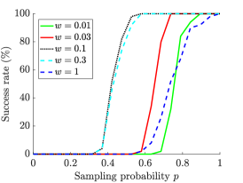
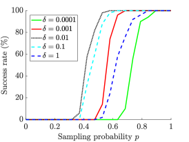
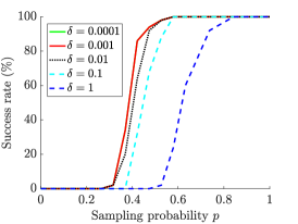
Figure 1a shows the results from the five algorithms, averaging the success probability over $50$ trials, where a successful trial is declared if $M$ is recovered up to a relative error of $10^{-3}$. The weighted matrix completion result is shown with a choice of $w=0.1$ and the reweighted nuclear norm heuristic (RNNH) result is shown with a choice of $\delta=0.01$. The results from these two algorithms with other values of $w$ and $\delta$ are shown in Figures 1b and 1c, respectively. We see in these plots that, with proper choices of $w$ and $\delta$, both the weighted algorithm and RNNH can substantially outperform standard matrix completion. In both cases, setting $w$ or $\delta$ too large or too small can hamper the performance. Moreover, in the best case, the weighted algorithm and RNNH perform comparably to each other. However, the weighted algorithm uses slightly weaker prior information, since it depends only on $(\widetilde{\operatorname{U}}_{r},\widetilde{\operatorname{V}}_{r})$ rather than all of $M^{\prime}$. The diagonal weighting algorithm also outperforms standard matrix completion, but its performance is not as strong as the weighted algorithm and RNNH, possibly because it relies on much less prior information (only the leverage scores of $M^{\prime}$). The least-squares algorithm does not succeed unless $p=1$ because one iteration of a least-squares algorithm is not enough to promote low-rank structure.

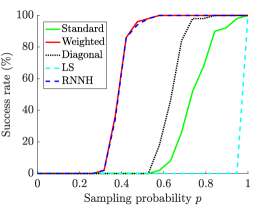
Figures 2a–2c show the results from a second experiment, where we use more accurate prior information. Specifically, in constructing $M^{\prime}$, we set $M^{\prime}=M+N$ where the entries of $N$ are independent Gaussian random variables with mean $0$ and variance $\sigma^{2}=10^{-6}$. The principal angles between the ground truth and prior knowledge subspaces are $u=\angle[\operatorname{U}_{r},{\widetilde{\operatorname{U}}}_{r}]=0.0099$ and $v=\angle[\operatorname{V}_{r},\widetilde{\operatorname{V}}_{r}]=0.0104$. We see a slight improvement in the performance of the weighted algorithm and RNNH, although the optimal choices of both $w$ and $\delta$ have decreased, as anticipated in Remarks 3 and 5. Although the best case performance is only slightly better than in the earlier experiment, we do observe a greater robustness to parameter choices: there are much wider ranges of $w$ and $\delta$ for which the algorithms perform well.

(a)

(b)

(c)

Figure 2: Matrix completion with stronger prior information, where the principal angles between the ground truth and prior knowledge subspaces are $u=\angle[\operatorname{U}_{r},{\widetilde{\operatorname{U}}}_{r}]=0.0099$ and $v=\angle[\operatorname{V}_{r},\widetilde{\operatorname{V}}_{r}]=0.0104$. (a) Comparison of standard (unweighted) matrix completion, weighted matrix completion with $w=0.03$, diagonal weighted matrix completion, weighted least-squares, and a weighted nuclear norm heuristic (RNNH) algorithm with $\delta=0.001$. (b) Weighted matrix completion with various weights $w$. (c) RNNH with various parameters $\delta$.

Figures 3a–3c repeat this experiment with less accurate prior information. In constructing $M^{\prime}$, we set $\sigma^{2}=0.0025$. The principal angles between the ground truth and prior knowledge subspaces are $u=\angle[\operatorname{U}_{r},{\widetilde{\operatorname{U}}}_{r}]=0.512$ and $v=\angle[\operatorname{V}_{r},\widetilde{\operatorname{V}}_{r}]=0.480$. Compared to the other experiments, we see a degradation in the performance of the weighted algorithm and RNNH, due to worse prior information. While both can still outperform standard matrix completion by choosing $w$ and $\delta$ suitably large, they can also both underperform standard matrix completion with an improper choice of parameters.

(a)

(b)

(c)

Figure 3: Matrix completion with weaker prior information, where the principal angles between the ground truth and prior knowledge subspaces are $u=\angle[\operatorname{U}_{r},{\widetilde{\operatorname{U}}}_{r}]=0.512$ and $v=\angle[\operatorname{V}_{r},\widetilde{\operatorname{V}}_{r}]=0.480$. (a) Comparison of standard (unweighted) matrix completion, weighted matrix completion with $w=0.3$, diagonal weighted matrix completion, weighted least-squares, and a weighted nuclear norm heuristic (RNNH) algorithm with $\delta=0.1$. (b) Weighted matrix completion with various weights $w$. (c) RNNH with various parameters $\delta$.

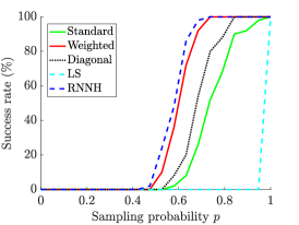
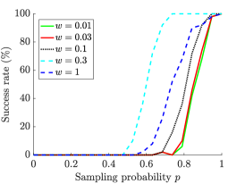
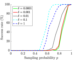
Figure 4 repeats the experiment from Figure 1a but with an equivalent number of random linear measurements in place of sampling the matrix entries. The algorithms are modified to perform matrix recovery instead of matrix completion, except we omit the diagonal weighting algorithm as the leverage score weighting algorithm in [4] was tailored to the problem of matrix completion. The relative algorithm performance is similar to other experiments.

Figure 4: Matrix recovery from random measurements with prior information, where $u=\angle[\operatorname{U}_{r},{\widetilde{\operatorname{U}}}_{r}]=0.119$ and $v=\angle[\operatorname{V}_{r},\widetilde{\operatorname{V}}_{r}]=0.086$. The figure shows a comparison of standard (unweighted) matrix completion, weighted matrix recovery with $w=0.3$, weighted least-squares, and a weighted nuclear norm heuristic (RNNH) algorithm with $\delta=0.01$.

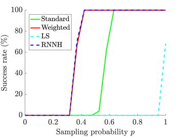
Figure 5 repeats the matrix completion experiment from Figure 1a but with a rank $r=2$ matrix rather than $r=4$. All algorithms perform better, as anticipated.

Figure 5: Matrix completion with prior information for a rank $r=2$ matrix. Here, $u=\angle[\operatorname{U}_{r},{\widetilde{\operatorname{U}}}_{r}]=0.075$ and $v=\angle[\operatorname{V}_{r},\widetilde{\operatorname{V}}_{r}]=0.064$. The algorithm parameters are $w=0.1$ and $\delta=0.01$.

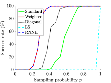
Figure 6 repeats the matrix completion experiment from Figure 1a but with a coherent matrix $M$ having larger leverage scores (the largest leverage score is $4.055$, as opposed to $2.211$ for the matrix used in the earlier experiment). This higher coherence hampers the performance of standard matrix completion and makes the advantages of the diagonal weighted algorithm more substantial. However, the weighted algorithm and RNNH still have the best performance in this experiment.

Figure 6: Matrix completion of a coherent matrix with prior information. Here, $u=\angle[\operatorname{U}_{r},{\widetilde{\operatorname{U}}}_{r}]=0.096$ and $v=\angle[\operatorname{V}_{r},\widetilde{\operatorname{V}}_{r}]=0.111$. The algorithm parameters are $w=0.1$ and $\delta=0.01$.

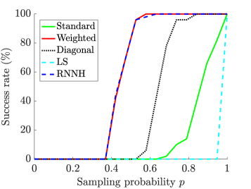
Finally, Figure 7 repeats the matrix completion experiment from Figure 1a but with a matrix sidelength of $n=40$ rather than $n=20$.

Figure 7: Matrix completion of a $40\times 40$ rank-$4$ matrix with prior information. Here, $u=\angle[\operatorname{U}_{r},{\widetilde{\operatorname{U}}}_{r}]=0.139$ and $v=\angle[\operatorname{V}_{r},\widetilde{\operatorname{V}}_{r}]=0.142$. The algorithm parameters are $w=0.1$ and $\delta=0.01$.

In all experiments in this section, we see that with proper parameter choices, both the weighted algorithm and RNNH can substantially outperform other techniques. Interestingly, the weighted algorithm and RNNH generally perform similarly to each other, although they originally came from different motivations (one as a means of employing prior information in a non-iterative fashion, the other as a step in an iterative algorithm that does not require prior information). Finally, as we have noted, the weighted algorithm uses slightly weaker prior information than RNNH, since it depends only on $(\widetilde{\operatorname{U}}_{r},\widetilde{\operatorname{V}}_{r})$ rather than all of $M^{\prime}$.

IV-B Iterative reweighting without prior information

Section IV-A focused on the question of how to best employ prior matrix information in one iteration of a matrix completion/recovery algorithm; this is indeed the main topic of this paper.

However, it is also possible to consider employing weighting in an iterative fashion, even when no prior information is available. In such a case, one begins by solving standard matrix completion/recovery, uses the result (call it $M^{\prime}$) as “prior” information to set weighting matrices, and then solves a weighted matrix completion/recovery program. As discussed in Section V, this is the original motivation for the RNNH that was evaluated in Section IV-A. In Figure 8, we compare an iterative, reweighted application of (19) to the iterative reweighted nuclear norm minimization algorithm from [19]. We see that after one weighted iteration, the algorithm from [19] has a slight performance advantage, while after four iterations (as prescribed in [19]), the two iterative algorithms perform similarly.

Figure 8: Matrix completion of a $20\times 20$ rank-$4$ matrix without prior information, through an iterative application of the weighted program (19) (labeled IRW) and an iterative application of the RNNH (labeled IRNN). Both algorithms are initialized using standard (unweighted) nuclear norm minimization, and the results after one and four subsequent weighted iterations are shown.

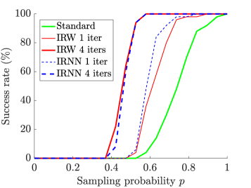
Overall, whether used in one iteration as a means of incorporating prior information or used in iterative fashion starting from an unweighted initialization, the weighted program in (19) and RNNH appear to perform similarly to each other across a range of problem instances. The goal of this paper is to quantify the benefit of incorporating prior information in one iteration of (19). It would be interesting to develop a similar analysis for RNNH, or to study the convergence of the iterative application of (19).

V Related Work

Programs similar to (18) and (19) have appeared in the literature before, and we wish to summarize here some of the related work. In [20, 21], the authors incorporate side information for matrix completion using nuclear norm minimization. However, their works differ from ours in that they assume perfect subspace information, which they use to reduce the dimension of the low-rank recovery problem (as well as the sample complexity). A later paper [22] supplements this recovery program with a correction term to account for imperfect side information. Theory is again provided which allows for a reduction in sample complexity; however, this theory is limited to randomly generated matrices and uses a different characterization of subspace accuracy than the principal angles we consider.

In [19], the authors considered the following non-convex program for rank minimization:

$$\begin{cases}\min_{X}\log\left(\det(X)\right)\\ X\in\mbox{C}.\end{cases}$$ (25)

Here, the feasible set $\mbox{C}\subset\mathbb{R}^{n\times n}$ is assumed to be convex. (Local) linearization of the above objective function leads to a majorization-minimization algorithm to solve Program (25), in which the $k$-th iteration takes the form of

$$\begin{cases}\min_{X}\left\|W_{1}^{k}XW_{2}^{k}\right\|_{*}\\ X\in\mbox{C},\end{cases}$$ (26)

for certain weight matrices $W_{1}^{k}$ and $W_{2}^{k}$. Convergence of this reweighted algorithm to a local minimum of Program (25) is known. See also [23] for a related problem.

In [7], the authors study the following program:

$$\min_{X\in\mathbb{R}^{n\times n}}\frac{1}{m}\left\|P_{\Omega}\left(X-Y\right)\right\|_{F}^{2}+\lambda_{N}\left\|AXB\right\|_{*}.$$ (27)

Here, $\Omega\subseteq[1:n]^{2}$ is a random index set of size $m$, and $P_{\Omega}(X)\in\mathbb{R}^{n\times n}$ retains the entries of $X$ on the index set $\Omega$ and sets the rest to zero. In addition, $Y=P_{\Omega}(M+E)$ where we take $M\in\mathbb{R}^{n\times n}$ to be rank-$r$ for simplicity, and the entries of $E\in\mathbb{R}^{n\times n}$ are independent zero-mean Gaussian random variables with variance $\sigma^{2}/n$. Lastly, $\lambda_{N}>0$ and $A,B\in\mathbb{R}^{n\times n}$ are both assumed to be invertible. Let $\widehat{M}\in\mathbb{R}^{n\times n}$ be a solution of Program (27). Then, Theorem 2 in the same reference establishes that

$$\left\|\widehat{M}-M\right\|_{F}^{2}\lesssim\alpha_{N}^{2}\max\left[1,\sigma^{2}\right]\frac{r\log n}{m},$$ (28)

with high probability and provided that $\lambda_{N}\gtrsim\sqrt{\frac{n\log n}{m}}$. Above,

$$\alpha_{N}:=n\cdot\frac{\left\|AMB^{*}\right\|_{\infty}}{\left\|AMB^{*}\right\|_{F}}.$$ (29)

By setting $A=Q_{\widetilde{\operatorname{U}}_{r},\lambda}$ and $B=Q_{\widetilde{\operatorname{V}}_{r},\rho}$ (see (17)), Program (27) will be equivalent to Program (19) for the right choice of $\lambda_{N}$. To compare (28) and Theorem 2, let $Q_{\widetilde{\operatorname{U}}_{r},\lambda}MQ^{*}_{\widetilde{\operatorname{V}}_{r},\rho}=U_{N,r}\Sigma_{N,r}V_{N,r}^{*}$ be the SVD of $AMB$ and note that

$$\alpha_{N}^{2} =n^{2}\cdot\frac{\left\|Q_{\widetilde{\operatorname{U}}_{r},\lambda}MQ_{\widetilde{\operatorname{V}}_{r},\rho}^{*}\right\|_{\infty}^{2}}{\left\|Q_{\widetilde{\operatorname{U}}_{r},\lambda}MQ_{\widetilde{\operatorname{V}}_{r},\rho}^{*}\right\|_{F}^{2}}$$

$$=n^{2}\cdot\frac{\left\|U_{N,r}\Sigma_{N,r}V_{N,r}^{*}\right\|_{\infty}^{2}}{\left\|U_{N,r}\Sigma_{N,r}V_{N,r}^{*}\right\|_{F}^{2}}$$

$$\leq n^{2}\cdot\frac{\left\|U_{N,r}\right\|_{2\rightarrow\infty}^{2}\cdot\left\|\Sigma_{N,r}\right\|^{2}\cdot\left\|V_{N,r}\right\|_{2\rightarrow\infty}^{2}}{\left\|\Sigma_{N,r}\right\|_{F}^{2}}$$

$$=n^{2}\cdot\frac{r^{2}\cdot\eta^{2}\left(Q_{\widetilde{\operatorname{U}}_{r},\lambda}MQ_{\widetilde{\operatorname{V}}_{r},\rho}^{*}\right)\left\|\Sigma_{N,r}\right\|^{2}}{n^{2}\left\|\Sigma_{N,r}\right\|_{F}^{2}}$$

$$\leq\frac{r\cdot\eta^{2}\left(Q_{\widetilde{\operatorname{U}}_{r},\lambda}MQ_{\widetilde{\operatorname{V}}_{r},\rho}^{*}\right)\left\|\Sigma_{N,r}\right\|^{2}}{\sigma_{r}^{2}\left(\Sigma_{N,r}\right)}$$

$$=r\cdot\eta^{2}\left(Q_{\widetilde{\operatorname{U}}_{r},\lambda}MQ_{\widetilde{\operatorname{V}}_{r},\rho}^{*}\right)\kappa^{2}\left(Q_{\widetilde{\operatorname{U}}_{r},\lambda}MQ_{\widetilde{\operatorname{V}}_{r},\rho}^{*}\right),$$ (30)

where $\eta(\cdot)$ and $\kappa(\cdot)$ return the coherence and condition number of a matrix, respectively. In particular, the above inequalities hold with equality when $U_{N,r},V_{N,r}$ are columns of the Fourier basis and the condition number of $Q_{\widetilde{\operatorname{U}}_{r},\lambda}MQ_{\widetilde{\operatorname{V}}_{r},\rho}^{*}$ equals one. Since coherence and condition number are both never smaller than one, we conclude that the right-hand side of (28) scales with $r^{2}$. This, in turn, forces $m$ (number of measurements) to scale with $r^{2}$. In contrast, the expected number of measurements required in Theorem 2 scales linearly with $r$. We must note that [7] itself was preceded by [24] where, among other contributions, a weighted program for matrix completion was studied with diagonal $A$ and $B$ in Program (27). A similar program was empirically studied in [25] in the context of collaborative filtering.

We would like to point out that our interest in weighted matrix recovery was inspired by [9], which we have previously mentioned in Section 1.1. In [9], weighted nuclear norm minimization has been successfully but heuristically applied to a “frequency continuation” matrix completion problem in seismic signal processing.

The ideas in this work have a precedent in compressive sensing and, more generally, sparse regression. In [26, 27], weighted $\ell_{1}$ minimization was proposed in order to incorporate partial information about the support; this was actually the inspiration for the weighted matrix completion algorithm in [9]. Originally, iterative reweighed $\ell_{1}$ minimization to enhance sparse recovery appeared in [28]. As our analysis in Sections VI-VIII indicates, extending these ideas to matrices requires different techniques and is substantially more involved.

VI Commons

In this section, we collect the necessary technical tools that are common to the analysis of both Programs (18) and (19). In particular, we find canonical decompositions for $M_{r}$ and the estimation error that takes the prior knowledge $({\widetilde{\operatorname{U}}}_{r},\widetilde{\operatorname{V}}_{r})$ into account by using standard tools from matrix analysis.

VI-A Canonical Decomposition

Central to the analysis is a canonical way of decomposing $M_{r}$ that takes the prior knowledge $({\widetilde{\operatorname{U}}}_{r},\widetilde{\operatorname{V}}_{r})$ into account. This result is well-known and a short proof is given in Appendix A for the sake of completeness [29]. Throughout, the empty blocks of matrices should be interpreted as filled with zeros. Also, in our notation, $I_{a}\in\mathbb{R}^{a\times a}$ is the identity matrix and $0_{a}\in\mathbb{R}^{a\times a}$ and $0_{a\times b}\in\mathbb{R}^{a\times b}$ are filled with zeros.

Lemma 3.

Consider a rank-$r$ matrix $M_{r}\in\mathbb{R}^{n\times n}$, and let $\operatorname{U}_{r}=\mbox{span}(M_{r})$ be the column span of $M_{r}$. Let ${\widetilde{\operatorname{U}}}_{r}$ be another $r$-dimensional subpsace in $\mathbb{R}^{n}$. Then, there exists $U_{r},\widetilde{U}_{r}\in\mathbb{R}^{n\times r}$, $U_{r}^{\prime},\widetilde{U}_{r}^{\prime}\in\mathbb{R}^{n\times r}$, and $U_{n-2r}^{\prime\prime}\in\mathbb{R}^{n\times(n-2r)}$ such that

$$\operatorname{U}_{r}=\mbox{span}\left(U_{r}\right),\quad{\widetilde{\operatorname{U}}}_{r}=\mbox{span}(\widetilde{U}_{r}),$$

and

$$B_{L} :=\left[\begin{array}[]{ccc}U_{r}&U^{\prime}_{r}&U^{\prime\prime}_{n-2r}\end{array}\right]\in\mathbb{R}^{n\times n},$$ (32)

$$\widetilde{B}_{L} :=\left[\begin{array}[]{ccc}\widetilde{U}_{r}&\widetilde{U}^{\prime}_{r}&U^{\prime\prime}_{n-2r}\end{array}\right]\in\mathbb{R}^{n\times n},$$ (34)

are both orthonormal bases for $\mathbb{R}^{n}$. Moreover, it holds that

$$B_{L}^{*}\widetilde{B}_{L}=\left[\begin{array}[]{ccc}\cos u&\sin u\\ -\sin u&\cos u\\ &&I_{n-2r}\end{array}\right],$$ (35)

where $u\in\mathbb{R}^{r\times r}$ is diagonal and contains the principal angles between ${\operatorname{U}}_{r}$ and ${{\widetilde{\operatorname{U}}}}_{r}$, in a non-increasing order: $\pi/2\geq u_{1}\geq u_{2}\geq\cdots\geq u_{r}\geq 0$. The diagonal matrix $\cos u$ is naturally defined as

$$\cos u:=\left[\begin{array}[]{cccc}\cos u_{1}\\ &\cos u_{2}\\ &&\ddots\\ &&&\cos u_{r}\end{array}\right]\in\mathbb{R}^{r\times r},$$

and $\sin u\in\mathbb{R}^{r\times r}$ is defined likewise. A similar construction exists for $\operatorname{V}_{r}=\mbox{span}(M_{r}^{*})$ and $\widetilde{\operatorname{V}}_{r}$, where we form the orthonormal bases $B_{R},\widetilde{B}_{R}\in\mathbb{R}^{n\times n}$ such that

$$B_{R}^{*}\widetilde{B}_{R}=\left[\begin{array}[]{ccc}\cos v&\sin v\\ -\sin v&\cos v\\ &&I_{n-2r}\end{array}\right].$$ (36)

As before, the diagonal of $v\in\mathbb{R}^{r\times r}$ contains the principal angles between $\operatorname{V}_{r}$ and $\widetilde{\operatorname{V}}_{r}$ in non-decreasing order.

Lemma 3 immediately implies that

$$\widetilde{U}_{r}=B_{L}\left[\begin{array}[]{c}\cos u\\ -\sin u\\ 0_{(n-2r)\times r}\end{array}\right],$$

which, in turn, allows us to derive the following expressions for orthogonal projections onto the subspace ${\widetilde{\operatorname{U}}}_{r}$ and its complement:

$$P_{{\widetilde{\operatorname{U}}}_{r}} =\widetilde{U}_{r}\widetilde{U}_{r}^{*}$$

$$=B_{L}\left[\begin{array}[]{ccc}\cos^{2}u&-\sin u\cdot\cos u\\ -\sin u\cdot\cos u&\sin^{2}u\\ &&0_{n-2r}\end{array}\right]B_{L}^{*},$$

$$P_{{\widetilde{\operatorname{U}}}_{r}^{\perp}} =I_{n}-P_{{\widetilde{\operatorname{U}}}_{r}}$$

$$=B_{L}\left[\begin{array}[]{ccc}\sin^{2}u&\sin u\cdot\cos u\\ \sin u\cdot\cos u&\cos^{2}u\\ &&I_{n-2r}\end{array}\right]B_{L}^{*}.$$

It also follows that

$$Q_{{\widetilde{\operatorname{U}}}_{r},\lambda}$$

$$=\lambda\cdot P_{{\widetilde{\operatorname{U}}}_{r}}+P_{{\widetilde{\operatorname{U}}}_{r}^{\perp}}$$

$$=B_{L}$$

$$\cdot\left[\begin{array}[]{ccc}\lambda\cos^{2}u+\sin^{2}u&(1-\lambda)\sin u\cdot\cos u\\ (1-\lambda)\sin u\cdot\cos u&\lambda\sin^{2}u+\cos^{2}u\\ &&I_{n-2r}\end{array}\right]B_{L}^{*},$$ (40)

where we used (17). We next mold the above expression for $Q_{{\widetilde{\operatorname{U}}}_{r},\lambda}$ into one that involves an upper-triangular matrix, as this will prove useful shortly. Define the orthonormal basis $O_{L}\in\mathbb{R}^{n\times n}$ as

$$O_{L} :=\left[\begin{array}[]{c}\left(\lambda\cos^{2}u+\sin^{2}u\right)\Delta_{L}^{-1}\\ (1-\lambda)\sin u\cdot\cos u\cdot\Delta_{L}^{-1}\\ 0_{(n-r)\times r}\end{array}\right.$$

$$\qquad\qquad\left.\begin{array}[]{cc}-(1-\lambda)\sin u\cdot\cos u\cdot\Delta_{L}^{-1}&0_{r\times(n-r)}\\ \left(\lambda\cos^{2}u+\sin^{2}u\right)\Delta_{L}^{-1}&0_{r\times(n-r)}\\ 0_{(n-r)\times r}&I_{n-2r}\end{array}\right],$$

$$\Delta_{L}:=\sqrt{\lambda^{2}\cos^{2}u+\sin^{2}u}\in\mathbb{R}^{r\times r},$$ (41)

where $\Delta_{L}$ is invertible because $\lambda>0$, by assumption. (It is easily verify that indeed $O_{L}O_{L}^{*}=I_{n}$.) We then rewrite (VI-A) as

$$Q_{{\widetilde{\operatorname{U}}}_{r},\lambda}$$

$$=B_{L}\left(O_{L}O_{L}^{*}\right)$$

$$\cdot\left[\begin{array}[]{ccc}\lambda\cos^{2}u+\sin^{2}u&(1-\lambda)\sin u\cdot\cos u\\ (1-\lambda)\sin u\cdot\cos u&\lambda\sin^{2}u+\cos^{2}u\\ &&I_{n-2r}\end{array}\right]B_{L}^{*}$$ (45)

$$=B_{L}O_{L}\left[\begin{array}[]{ccc}\Delta_{L}&(1-\lambda^{2})\sin u\cdot\cos u\cdot\Delta_{L}^{-1}\\ &\lambda\Delta_{L}^{-1}\\ &&I_{n-2r}\end{array}\right]B_{L}^{*}$$ (49)

$$=:B_{L}O_{L}\left[\begin{array}[]{ccc}L_{11}&L_{12}\\ &L_{22}\\ &&I_{n-2r}\end{array}\right]B_{L}^{*}$$ (53)

$$=:B_{L}O_{L}LB_{L}^{*},$$ (54)

where $L\in\mathbb{R}^{n\times n}$ is an upper-triangular matrix with blocks $L_{11},L_{12},L_{22}\in\mathbb{R}^{r\times r}$ and defined as

$$L :=\left[\begin{array}[]{ccc}L_{11}&L_{12}\\ &L_{22}\\ &&I_{n-2r}\end{array}\right]$$ (58)

$$=\left[\begin{array}[]{ccc}\Delta_{L}&\left(1-\lambda^{2}\right)\sin u\cdot\cos u\cdot\Delta_{L}^{-1}\\ &\lambda\Delta_{L}^{-1}&\\ &&I_{n-2r}\end{array}\right].$$ (62)

In the third line of (54), we used the fact that $O_{L}O_{L}^{*}=I_{n}$. Because $B_{L},O_{L}$ are both orthonormal bases, we record that

$$\left\|Q_{{\widetilde{\operatorname{U}}}_{r},\lambda}\right\|=\|L\|=1.\qquad\mbox{(see \eqref{eq:def of Qs} and \eqref{eq:conn btw Q and L})}$$ (63)

We can perform the same calculations for the row spaces and, in particular, define $R\in\mathbb{R}^{n\times n}$ as

$$R :=\left[\begin{array}[]{ccc}R_{11}&R_{12}\\ &R_{22}\\ &&I_{n-2r}\end{array}\right]$$ (67)

$$=\left[\begin{array}[]{ccc}\Delta_{R}&(1-\rho^{2})\sin v\cdot\cos v\cdot\Delta_{R}^{-1}\\ &\rho\Delta_{R}^{-1}\\ &&I_{n-2r}\end{array}\right],$$ (71)

with $\Delta_{R}=\sqrt{\rho^{2}\cos^{2}v+\sin^{2}v}\in\mathbb{R}^{n\times n}$. With these calculations in mind, for an arbitrary matrix $H\in\mathbb{R}^{n\times n}$, we find the crucial decomposition

$$Q_{{\widetilde{\operatorname{U}}}_{r},\lambda}\cdot H\cdot Q_{\widetilde{\operatorname{V}}_{r},\rho}$$

$$=B_{L}O_{L}L\left(B_{L}^{*}HB_{R}\right)R^{*}O_{R}^{*}B_{R}^{*}\,\,\left(\mbox{\eqref{eq:conn btw Q and L} and }Q_{\widetilde{\operatorname{V}}_{r},\rho}=Q_{\widetilde{\operatorname{V}}_{r},\rho}^{*}\right)$$

$$=:B_{L}O_{L}L\overline{H}R^{*}O_{R}^{*}B_{R}^{*}\qquad\left(\overline{H}:=B_{L}^{*}HB_{R}\right)$$

$$=:B_{L}O_{L}L\left[\begin{array}[]{ccc}\overline{H}_{11}&\overline{H}_{12}&\overline{H}_{13}\\ \overline{H}_{21}&\overline{H}_{22}&\overline{H}_{23}\\ \overline{H}_{31}&\overline{H}_{32}&\overline{H}_{33}\end{array}\right]R^{*}O_{R}^{*}B_{R}^{*},$$ (75)

with $\overline{H}_{11},\overline{H}_{22}\in\mathbb{R}^{r\times r}$ and $\overline{H}_{33}\in\mathbb{R}^{(n-2r)\times(n-2r)}$ being the diagonal blocks of $\overline{H}$. Moreover, from Lemma 3, recall that

$$\mbox{span}\left(M_{r}\right)=\mbox{span}\left(U_{r}\right),\quad\mbox{span}\left(M_{r}^{*}\right)=\mbox{span}\left(V_{r}\right),$$ (76)

which allows us to record that

$$Q_{{\widetilde{\operatorname{U}}}_{r},\lambda}\cdot M_{r}\cdot Q_{\widetilde{\operatorname{V}}_{r},\rho}$$

$$=B_{L}O_{L}L\left(B_{L}^{*}M_{r}B_{R}\right)R^{*}O_{R}^{*}B_{R}^{*}\qquad\mbox{(see \eqref{eq:conn btw Q and L})}$$

$$=:B_{L}O_{L}L\overline{M}_{r}R^{*}O_{R}^{*}B_{R}^{*}\qquad\left(\overline{M}_{r}:=B_{L}^{*}M_{r}B_{R}\right)$$

$$=:B_{L}O_{L}L\left[\begin{array}[]{cc}\overline{M}_{r,11}\\ &0_{n-r}\\ \end{array}\right]R^{*}O_{R}^{*}B_{R}^{*}\qquad\mbox{(see \eqref{eq:M is single block})}$$ (79)

$$=B_{L}O_{R}\left[\begin{array}[]{cc}L_{11}\overline{M}_{r,11}R_{11}\\ &0_{n-r}\end{array}\right]$$ (82)

$$\qquad\qquad\qquad\cdot O_{R}^{*}B_{R}^{*}.\qquad\left(\mbox{\eqref{eq:def of Wu} and }R_{11}=R_{11}^{*}\right)$$ (83)

In the last line above, we benefited from the fact that, by construction, both $L$ and $R$ are upper-triangular matrices. Note also that $\overline{M}_{r,11}=U_{r}^{*}M_{r}V_{r}$, as defined above, is not necessarily diagonal. For future reference, the following useful inequalities are proved in Appendix B.

Lemma 4.

With $L$ and its blocks $L_{11},L_{12},L_{22}$ defined in (62), it holds that

$$\left\|L_{11}\right\|=\left\|\Delta_{L}\right\|\leq\sqrt{\lambda^{2}\cos^{2}u_{1}+\sin^{2}u_{1}},$$

$$\|L_{12}\| \leq\frac{\left(1-\lambda^{2}\right)\sin u_{1}}{\sqrt{\lambda^{2}\cos^{2}u_{1}+\sin^{2}u_{1}}}\leq 1-\lambda^{2},$$

$$\left\|I_{r}-L_{22}\right\| \leq\frac{\sqrt{1-\lambda^{2}}\sin u_{1}}{\sqrt{\lambda^{2}\cos^{2}u_{1}+\sin^{2}u_{1}}}\leq\sqrt{1-\lambda^{2}},$$

$$\left\|\left[\begin{array}[]{cc}L_{11}&L_{12}\end{array}\right]\right\|^{2} \leq\frac{\lambda^{4}\cos^{2}u_{1}+\sin^{2}u_{1}}{\lambda^{2}\cos^{2}u_{1}+\sin^{2}u_{1}}\leq 1,$$

$$\left\|\left[\begin{array}[]{cc}L_{22}-I_{r}&L_{12}\end{array}\right]\right\|^{2} \leq\frac{2(1-\lambda^{2})\sin^{2}u_{1}}{\lambda^{2}\cos^{2}u_{1}+\sin^{2}u_{1}},$$ (85)

where $u_{1}$ is the largest principal angle between $r$-dimensional subspaces $\operatorname{U}_{r}$ and ${\widetilde{\operatorname{U}}}_{r}$. Similar bounds hold for $R$ and its blocks, $R_{11},R_{12},R_{22}$.

VI-B Support

Let $M_{r}$ be a rank-$r$ truncation of $M\in\mathbb{R}^{n\times n}$ (obtained via SVD) and consider the decomposition

$$M=M_{r}+M_{r^{+}}=U_{r}\overline{M}_{r,11}V_{r}^{*}+M_{r^{+}},$$

where $U_{r},V_{r}\in\mathbb{R}^{n\times r}$ (with orthonormal columns) span column and row spaces of $M_{r}$, and $\overline{M}_{11}\in\mathbb{R}^{r\times r}$ is rank-$r$ but not necessary diagonal. Let $\operatorname{U}_{r}=\mbox{span}(U_{r})=\mbox{span}(M_{r})$ and $\operatorname{V}_{r}=\mbox{span}(V_{r})=\mbox{span}(M_{r}^{*})$. Then, the support of $M_{r}\in\mathbb{R}^{n\times n}$ is the linear subspace $\operatorname{T}\subset\mathbb{R}^{n\times n}$ defined as

$$\operatorname{T}=\left\{Z\in\mathbb{R}^{n\times n}\,:\,Z=P_{\operatorname{U}_{r}}\cdot Z+Z\cdot P_{\operatorname{V}_{r}}-P_{\operatorname{U}_{r}}\cdot Z\cdot P_{\operatorname{V}_{r}}\right\},$$ (86)

where $P_{\operatorname{U}_{r}},P_{\operatorname{V}_{r}}\in\mathbb{R}^{n\times n}$ are orthogonal projection onto $\operatorname{U}_{r},\operatorname{V}_{r}$, respectively. For the record, the orthogonal projection onto $\operatorname{T}$ and its complement $\operatorname{T}^{\perp}$ take $Z\in\mathbb{R}^{n\times n}$ to

$$\mathcal{P}_{\operatorname{T}}(Z)=P_{\operatorname{U}_{r}}\cdot Z+Z\cdot P_{\operatorname{V}_{r}}-P_{\operatorname{U}_{r}}\cdot Z\cdot P_{\operatorname{V}_{r}},$$

$$\mathcal{P}_{\operatorname{T}^{\perp}}(Z)=P_{\operatorname{U}_{r}^{\perp}}\cdot Z\cdot P_{\operatorname{V}_{r}^{\perp}},$$

respectively. As suggested above, throughout we reserve the calligraphic font for matrix operators. Note that, using Lemma 3, we can express $\operatorname{T}$ equivalently as

$$\operatorname{T} =\left\{Z\in\mathbb{R}^{n\times n}\,:\,Z=B_{L}\overline{Z}B_{R}^{*},\quad\overline{Z}=\left[\begin{array}[]{cc}\overline{Z}_{11}&\overline{Z}_{12}\\ \overline{Z}_{21}&0_{n-r}\end{array}\right]\right\}$$ (88)

$$=:B_{L}\cdot\overline{\operatorname{T}}\cdot B_{R}^{*},$$ (89)

where, to be clear, the new subspace $\overline{\operatorname{T}}\subset\mathbb{R}^{n\times n}$ is the support of $\overline{M}_{r}:=B_{L}^{*}M_{r}B_{R}$ and is defined as

$$\overline{\operatorname{T}}=\left\{\overline{Z}\in\mathbb{R}^{n\times n}\,:\,\overline{Z}=\left[\begin{array}[]{cc}\overline{Z}_{11}&\overline{Z}_{12}\\ \overline{Z}_{21}&0_{n-r}\end{array}\right]\right\}.$$ (90)

Also note that, for arbitrary

$$\overline{Z}=\left[\begin{array}[]{cc}\overline{Z}_{11}&\overline{Z}_{12}\\ \overline{Z}_{21}&\overline{Z}_{22}\end{array}\right]\in\mathbb{R}^{n\times n},$$

with $\overline{Z}_{11}\in\mathbb{R}^{r\times r},\overline{Z}_{22}\in\mathbb{R}^{(n-r)\times(n-r)}$, the orthogonal projection onto $\overline{\operatorname{T}}$ and its complement simply take $\overline{Z}$ to

$$\mathcal{P}_{\overline{\operatorname{T}}}\left(\overline{Z}\right)=\left[\begin{array}[]{cc}\overline{Z}_{11}&\overline{Z}_{12}\\ \overline{Z}_{21}&0_{n-r}\end{array}\right],$$

$$\mathcal{P}_{\overline{\operatorname{T}}^{\perp}}\left(\overline{Z}\right)=\left[\begin{array}[]{cc}0_{r}\\ &\overline{Z}_{22}\end{array}\right],$$ (91)

respectively. Lastly, we record the following connection: For arbitrary $Z\in\mathbb{R}^{n\times n}$ and with $\overline{Z}=B_{L}^{*}ZB_{R}$, we have that

$$\mathcal{P}_{\operatorname{T}}(Z)=B_{L}\cdot\mathcal{P}_{\overline{\operatorname{T}}}\left(\overline{Z}\right)\cdot B_{R}^{*},$$

$$\mathcal{P}_{\operatorname{T}^{\perp}}(Z)=B_{L}\cdot\mathcal{P}_{\overline{\operatorname{T}}^{\perp}}\left(\overline{Z}\right)\cdot B_{R}^{*}.$$ (92)

VII Analysis for Matrix Recovery

In this section, we study Program (18) in detail and eventually prove Theorem 1. First, in Section VII-A, we establish a variant of the well-known nullspace property for Program (18) which loosely states that the recovery error in Program (18) is concentrated along the subspace $\operatorname{T}$, namely the support of $M_{r}$. Using this property, we then complete the proof of Theorem 1 in Section VII-B by breaking down the error into smaller components to which we can apply the RIP.

VII-A Nullspace Property

For solution $\widehat{M}$, let $H:=\widehat{M}-M$ be the error. By feasibility of $M$ and optimality of $\widehat{M}=M+H$ in Program (18), we have that

$$\left\|Q_{\widetilde{\operatorname{U}}_{r},\lambda}\left(M+H\right)Q_{\widetilde{\operatorname{V}}_{r},\rho}\right\|_{*}\leq\left\|Q_{\widetilde{\operatorname{U}}_{r},\lambda}MQ_{\widetilde{\operatorname{V}}_{r},\rho}\right\|_{*}.$$ (93)

Recall that $M=M_{r}+M_{r^{+}}$. With the decomposition of $M_{r}$ in (83) at hand, the right-hand side above is then bounded follows:

$$\left\|Q_{\widetilde{\operatorname{U}}_{r},\lambda}MQ_{\widetilde{\operatorname{V}}_{r},\rho}\right\|_{*}$$

$$\leq\left\|Q_{\widetilde{\operatorname{U}}_{r},\lambda}M_{r}Q_{\widetilde{\operatorname{V}}_{r},\rho}\right\|_{*}+\left\|Q_{\widetilde{\operatorname{U}}_{r},\lambda}M_{r^{+}}Q_{\widetilde{\operatorname{V}}_{r},\rho}\right\|_{*}$$

$$=\left\|B_{L}O_{L}^{*}\left[\begin{array}[]{cc}L_{11}\overline{M}_{r,11}R_{11}\\ &0_{n-r}\end{array}\right]O_{R}^{*}B_{R}^{*}\right\|_{*}$$ (96)

$$\qquad\qquad+\left\|Q_{\widetilde{\operatorname{U}}_{r},\lambda}M_{r^{+}}Q_{\widetilde{\operatorname{V}}_{r},\rho}\right\|_{*}\qquad\mbox{(see \eqref{eq:M decompose})}$$

$$=\left\|\left[\begin{array}[]{cc}L_{11}\overline{M}_{r,11}R_{11}\\ &0_{n-r}\end{array}\right]\right\|_{*}+\left\|Q_{\widetilde{\operatorname{U}}_{r},\lambda}M_{r^{+}}Q_{\widetilde{\operatorname{V}}_{r},\rho}\right\|_{*}$$ (99)

$$=\left\|L\overline{M}R^{*}\right\|_{*}+\left\|Q_{\widetilde{\operatorname{U}}_{r},\lambda}M_{r^{+}}Q_{\widetilde{\operatorname{V}}_{r},\rho}\right\|_{*},\qquad\mbox{(see \eqref{eq:M decompose})}$$ (100)

where the first inequality above uses $M=M_{r}+M_{r^{+}}$ and the triangle inequality. The second identity uses the rotational invariance of the nuclear norm. In the last line, we used the fact that $B_{L},B_{R},O_{L},O_{R}$ are all orthonormal bases. Using the decomposition of $H$ in (75), the left hand side of (209) can also be bounded as follows:

$$\left\|Q_{\widetilde{\operatorname{U}}_{r},\lambda}\left(M+H\right)Q_{\widetilde{\operatorname{V}},\rho}\right\|_{*}$$

$$\geq\left\|Q_{\widetilde{\operatorname{U}}_{r},\lambda}\left(M_{r}+H\right)Q_{\widetilde{\operatorname{V}}_{r},\rho}\right\|_{*}-\left\|Q_{\widetilde{\operatorname{U}}_{r},\lambda}M_{r^{+}}Q_{\widetilde{\operatorname{V}}_{r},\rho}\right\|_{*}$$

$$=\left\|B_{L}O_{L}L\left(\overline{M}_{r}+\overline{H}\right)R^{*}O_{R}^{*}B_{R}^{*}\right\|_{*}-\left\|Q_{\widetilde{\operatorname{U}}_{r},\lambda}M_{r^{+}}Q_{\widetilde{\operatorname{V}}_{r},\rho}\right\|_{*}$$

$$=\left\|L\overline{M}_{r}R^{*}+L\overline{H}R^{*}\right\|_{*}-\left\|Q_{\widetilde{\operatorname{U}}_{r},\lambda}M_{r^{+}}Q_{\widetilde{\operatorname{V}}_{r},\rho}\right\|_{*}$$

$$=\left\|L\overline{M}_{r}R^{*}+L\mathcal{P}_{\overline{\operatorname{T}}}\left(\overline{H}\right)R^{*}+L\mathcal{P}_{\overline{\operatorname{T}}^{\perp}}\left(\overline{H}\right)R^{*}\right\|_{*}$$

$$\qquad-\left\|Q_{\widetilde{\operatorname{U}}_{r},\lambda}M_{r^{+}}Q_{\widetilde{\operatorname{V}}_{r},\rho}\right\|_{*}$$

$$=\left\|L\overline{M}_{r}R^{*}+L\mathcal{P}_{\overline{\operatorname{T}}}\left(\overline{H}\right)R^{*}+L\mathcal{P}_{\overline{\operatorname{T}}^{\perp}}\left(\overline{H}\right)R^{*}\right.$$

$$\qquad\qquad\left.-\mathcal{P}_{\overline{\operatorname{T}}^{\perp}}\left(\overline{H}\right)+\mathcal{P}_{\operatorname{T}^{\perp}}\left(\overline{H}\right)\right\|_{*}-\left\|Q_{\widetilde{\operatorname{U}}_{r},\lambda}M_{r^{+}}Q_{\widetilde{\operatorname{V}}_{r},\rho}\right\|_{*}.$$

Above, the second line uses $M=M_{r}+M_{r^{+}}$ and the the triangle inequality. The third line uses (75) and (83). The fourth line uses the rotational invariance of the nuclear norm. We continue by writing that

$$\left\|Q_{\widetilde{\operatorname{U}}_{r},\lambda}\left(M+H\right)Q_{\widetilde{\operatorname{V}},\rho}\right\|_{*}$$

$$=\left\|L\overline{M}_{r}R^{*}+L\mathcal{P}_{\overline{\operatorname{T}}}\left(\overline{H}\right)R^{*}+L\left[\begin{array}[]{ccc}0_{r}\\ &\overline{H}_{22}&\overline{H}_{23}\\ &\overline{H}_{32}&\overline{H}_{33}\end{array}\right]R^{*}\right.$$

$$\qquad\qquad\left.-\left[\begin{array}[]{ccc}0_{r}\\ &\overline{H}_{22}&\overline{H}_{23}\\ &\overline{H}_{32}&\overline{H}_{33}\end{array}\right]+\mathcal{P}_{\overline{\operatorname{T}}^{\perp}}\left(\overline{H}\right)\right\|_{*}$$

$$\qquad\qquad-\left\|Q_{\widetilde{\operatorname{U}}_{r},\lambda}M_{r^{+}}Q_{\widetilde{\operatorname{V}}_{r},\rho}\right\|_{*}\quad\mbox{(see \eqref{eq:PT PTperp})}$$

$$=:\left\|L\overline{M}_{r}R^{*}+L\mathcal{P}_{\overline{\operatorname{T}}}\left(\overline{H}\right)R^{*}+L\overline{H}^{\prime}R^{*}-\overline{H}^{\prime}+\mathcal{P}_{\overline{\operatorname{T}}^{\perp}}\left(\overline{H}\right)\right\|_{*}$$

$$\qquad-\left\|Q_{\widetilde{\operatorname{U}}_{r},\lambda}M_{r^{+}}Q_{\widetilde{\operatorname{V}}_{r},\rho}\right\|_{*}\qquad\mbox{(see \eqref{eq:def of H'})}$$

$$\geq\left\|L\overline{M}_{r}R^{*}+\mathcal{P}_{\overline{\operatorname{T}}^{\perp}}\left(\overline{H}\right)\right\|_{*}-\left\|L\mathcal{P}_{\overline{\operatorname{T}}}\left(\overline{H}\right)R^{*}\right\|_{*}$$

$$\qquad-\left\|L\overline{H}^{\prime}R^{*}-\overline{H}^{\prime}\right\|_{*}-\left\|Q_{\widetilde{\operatorname{U}}_{r},\lambda}M_{r^{+}}Q_{\widetilde{\operatorname{V}},\rho}\right\|_{*},$$

where the last line uses the triangle inequality. To be concrete, above we defined

$$\overline{H}^{\prime}:=\left[\begin{array}[]{ccc}0_{r}\\ &\overline{H}_{22}&\overline{H}_{23}\\ &\overline{H}_{32}&0_{n-2r}\end{array}\right]\in\mathbb{R}^{n\times n}.$$ (101)

Consequently,

$$\left\|Q_{\widetilde{\operatorname{U}}_{r},\lambda}\left(M+H\right)Q_{\widetilde{\operatorname{V}},\rho}\right\|_{*}$$

$$=\left\|\left[\begin{array}[]{ccc}L_{11}\overline{M}_{r,11}R_{11}\\ &\overline{H}_{22}&\overline{H}_{23}\\ &\overline{H}_{32}&\overline{H}_{33}\end{array}\right]\right\|_{*}-\left\|L\mathcal{P}_{\overline{\operatorname{T}}}\left(\overline{H}\right)R^{*}\right\|_{*}$$ (105)

$$\qquad\qquad-\left\|L\overline{H}^{\prime}R^{*}-\overline{H}^{\prime}\right\|_{*}-\left\|Q_{\widetilde{\operatorname{U}}_{r},\lambda}M_{r^{+}}Q_{\widetilde{\operatorname{V}}_{r},\rho}\right\|_{*}$$

$$=\left\|\left[\begin{array}[]{ccc}L_{11}\overline{M}_{r,11}R_{11}\\ &0_{r}\\ &&0_{n-2r}\end{array}\right]\right\|_{*}$$ (109)

$$\qquad+\left\|\left[\begin{array}[]{ccc}0_{r}\\ &\overline{H}_{22}&\overline{H}_{23}\\ &\overline{H}_{32}&\overline{H}_{33}\end{array}\right]\right\|_{*}-\left\|L\mathcal{P}_{\overline{\operatorname{T}}}\left(\overline{H}\right)R^{*}\right\|_{*}$$ (113)

$$\qquad-\left\|L\overline{H}^{\prime}R^{*}-\overline{H}^{\prime}\right\|_{*}-\left\|Q_{\widetilde{\operatorname{U}}_{r},\lambda}M_{r^{+}}Q_{\widetilde{\operatorname{V}}_{r},\rho}\right\|_{*}$$

$$=\left\|L\overline{M}R^{*}\right\|_{*}+\left\|\mathcal{P}_{\overline{\operatorname{T}}^{\perp}}\left(\overline{H}\right)\right\|_{*}-\left\|L\mathcal{P}_{\overline{\operatorname{T}}}\left(\overline{H}\right)R^{*}\right\|_{*}$$

$$\qquad-\left\|L\overline{H}^{\prime}R^{*}-\overline{H}^{\prime}\right\|_{*}-\left\|Q_{\widetilde{\operatorname{U}}_{r},\lambda}M_{r^{+}}Q_{\widetilde{\operatorname{V}}_{r},\rho}\right\|_{*}.$$ (114)

Above, we used (83) and (91) twice. In the second identity in (114), we used the fact that $\|A+B\|_{*}=\|A\|_{*}+\|B\|_{*}$ whenever both column and row spaces of $A$ are orthogonal to those of $B$, namely when $A^{*}B=AB^{*}=0$. Now combining (93) with the bounds in (100) and (114) yields that

$$\left\|\mathcal{P}_{\overline{\operatorname{T}}^{\perp}}\left(\overline{H}\right)\right\|_{*} \leq\left\|L\mathcal{P}_{\overline{\operatorname{T}}}\left(\overline{H}\right)R^{*}\right\|_{*}+\left\|L\overline{H}^{\prime}R^{*}-\overline{H}^{\prime}\right\|_{*}$$

$$\qquad\qquad+2\left\|Q_{\widetilde{\operatorname{U}}_{r},\lambda}M_{r^{+}}Q_{\widetilde{\operatorname{V}}_{r},\rho}\right\|_{*}.$$ (115)

We next simplify the terms in the above inequality. First, notice that

$$\left[\begin{array}[]{ccc}0_{r}&&\\ &L_{22}&\\ &&I_{n-2r}\end{array}\right]\mathcal{P}_{\overline{\operatorname{T}}}\left(\overline{H}\right)\left[\begin{array}[]{ccc}0_{r}&&\\ &R_{22}&\\ &&I_{n-2r}\end{array}\right]$$ (122)

$$=\left[\begin{array}[]{ccc}0_{r}&&\\ &L_{22}&\\ &&I_{n-2r}\end{array}\right]\left[\begin{array}[]{ccc}\overline{H}_{11}&\overline{H}_{12}&\overline{H}_{13}\\ \overline{H}_{21}&0_{r}&\\ \overline{H}_{31}&&0_{n-2r}\end{array}\right]$$ (129)

$$\qquad\qquad\cdot\left[\begin{array}[]{ccc}0_{r}&&\\ &R_{22}&\\ &&I_{n-2r}\end{array}\right]\qquad\mbox{(see \eqref{eq:PT PTperp})}$$ (133)

$$=0_{n},$$ (134)

which, in turn, allows us to simplify the first norm on the right-hand side of (115) as follows:

$$\left\|L\mathcal{P}_{\overline{\operatorname{T}}}\left(\overline{H}\right)R^{*}\right\|_{*}$$

$$=\left\|\left[\begin{array}[]{ccc}L_{11}&L_{12}\\ &L_{22}\\ &&I_{n-2r}\end{array}\right]\mathcal{P}_{\overline{\operatorname{T}}}\left(\overline{H}\right)\left[\begin{array}[]{ccc}R_{11}\\ R_{12}^{*}&R_{22}\\ &&I_{n-2r}\end{array}\right]\right.$$

$$\left.-\left[\begin{array}[]{ccc}0_{r}\\ &L_{22}\\ &&I_{n-2r}\end{array}\right]\mathcal{P}_{\overline{\operatorname{T}}}\left(\overline{H}\right)\left[\begin{array}[]{ccc}0_{r}\\ &R_{22}\\ &&I_{n-2r}\end{array}\right]\right\|_{*},$$

where we used (134). Then we continue by writing that

$$\left\|L\mathcal{P}_{\overline{\operatorname{T}}}\left(\overline{H}\right)R^{*}\right\|_{*}$$

$$=\left\|\left[\begin{array}[]{ccc}L_{11}&L_{12}\\ &0_{r}\\ &&0_{n-2r}\end{array}\right]\mathcal{P}_{\overline{\operatorname{T}}}\left(\overline{H}\right)R^{*}\right.$$

$$\left.+\left[\begin{array}[]{ccc}0_{r}\\ &L_{22}\\ &&I_{n-2r}\end{array}\right]\mathcal{P}_{\overline{\operatorname{T}}}\left(\overline{H}\right)\left[\begin{array}[]{ccc}R_{11}\\ R_{12}^{*}&0_{r}\\ &&0_{n-2r}\end{array}\right]\right\|_{*},$$

in which we applied (157). Consequently,

$$\left\|L\mathcal{P}_{\overline{\operatorname{T}}}\left(\overline{H}\right)R^{*}\right\|_{*}$$

$$\leq\left\|\left[\begin{array}[]{ccc}L_{11}&L_{12}\\ &0_{r}\\ &&0_{n-2r}\end{array}\right]\mathcal{P}_{\overline{\operatorname{T}}}\left(\overline{H}\right)R^{*}\right\|_{*}$$ (138)

$$+\left\|\left[\begin{array}[]{ccc}0_{r}\\ &L_{22}\\ &&I_{n-2r}\end{array}\right]\mathcal{P}_{\overline{\operatorname{T}}}\left(\overline{H}\right)\left[\begin{array}[]{ccc}R_{11}\\ R_{12}^{*}&0_{r}\\ &&0_{n-2r}\end{array}\right]\right\|_{*}$$ (145)

$$\leq\left\|\left[\begin{array}[]{cc}L_{11}&L_{12}\end{array}\right]\right\|\left\|\mathcal{P}_{\overline{\operatorname{T}}}\left(\overline{H}\right)\right\|_{*}\|R\|$$ (147)

$$\qquad+\max\left[\|L_{22}\|,1\right]\left\|\mathcal{P}_{\overline{\operatorname{T}}}\left(\overline{H}\right)\right\|_{*}\left\|\left[\begin{array}[]{cc}R_{11}&R_{12}\end{array}\right]\right\|$$ (149)

$$\leq\left\|\left[\begin{array}[]{cc}L_{11}&L_{12}\end{array}\right]\right\|\left\|\mathcal{P}_{\overline{\operatorname{T}}}\left(\overline{H}\right)\right\|_{*}$$ (151)

$$\qquad\qquad+\left\|\mathcal{P}_{\overline{\operatorname{T}}}\left(\overline{H}\right)\right\|_{*}\left\|\left[\begin{array}[]{cc}R_{11}&R_{12}\end{array}\right]\right\|$$ (153)

$$=\left(\left\|\left[\begin{array}[]{cc}L_{11}&L_{12}\end{array}\right]\right\|+\left\|\left[\begin{array}[]{cc}R_{11}&R_{12}\end{array}\right]\right\|\right)\left\|\mathcal{P}_{\overline{\operatorname{T}}}\left(\overline{H}\right)\right\|_{*}.$$ (156)

The second inequality above uses the fact that $\|AB\|_{*}\leq\|A\|\cdot\|B\|_{*}$ for all conforming matrices $A,B$. The last inequality uses (62), (63), and the observation that $\left\|L_{22}\right\|\leq\|L\|$. In the second inequality, we also used the so-called polarization identity

$$AZC-BZD=(A-B)ZC+BZ(C-D),$$ (157)

for conforming matrices $A,B,C,D,Z$. The second norm on the right-hand side of (115) may also be bounded as follows:

$$\left\|L\overline{H}^{\prime}R^{*}-\overline{H}^{\prime}\right\|_{*}$$

$$=\left\|\left[\begin{array}[]{ccc}L_{11}&L_{12}\\ &L_{22}\\ &&I_{n-2r}\end{array}\right]\overline{H}^{\prime}\left[\begin{array}[]{ccc}R_{11}\\ R_{12}^{*}&R_{22}\\ &&I_{n-2r}\end{array}\right]\right.$$

$$\qquad\left.-\left[\begin{array}[]{ccc}L_{11}\\ &I_{r}\\ &&I_{n-2r}\end{array}\right]\overline{H}^{\prime}\left[\begin{array}[]{ccc}R_{11}\\ &I_{r}\\ &&I_{n-2r}\end{array}\right]\right\|_{*}$$

$$=\left\|\left[\begin{array}[]{ccc}0_{r}&L_{12}\\ &L_{22}-I_{r}\\ &&0_{n-2r}\end{array}\right]\overline{H}^{\prime}R^{*}\right.$$

$$\left.\,-\left[\begin{array}[]{ccc}L_{11}\\ &I_{r}\\ &&I_{n-2r}\end{array}\right]\overline{H}^{\prime}\left[\begin{array}[]{ccc}0_{r}\\ R_{12}^{*}&R_{22}-I_{r}\\ &&0_{n-2r}\end{array}\right]\right\|_{*},$$

Above, the first identity uses (62). and (101). The second identity employs (157). We continue by applying the triangle inequality to find that

$$\left\|L\overline{H}^{\prime}R^{*}-\overline{H}^{\prime}\right\|_{*}$$

$$\leq\left\|\left[\begin{array}[]{ccc}0_{r}&L_{12}\\ &L_{22}-I_{r}\\ &&0_{n-2r}\end{array}\right]\overline{H}^{\prime}R^{*}\right\|_{*}$$

$$+\left\|\left[\begin{array}[]{ccc}L_{11}\\ &I_{r}\\ &&I_{n-2r}\end{array}\right]\overline{H}^{\prime}\left[\begin{array}[]{ccc}0_{r}\\ R_{12}^{*}&R_{22}-I_{r}\\ &&0_{n-2r}\end{array}\right]\right\|_{*},$$

and, consequently,

$$\left\|L\overline{H}^{\prime}R^{*}-\overline{H}^{\prime}\right\|_{*}$$

$$\leq\left\|\left[\begin{array}[]{cc}L_{12}^{*}&L_{22}-I_{r}\end{array}\right]\right\|\left\|\overline{H}^{\prime}\right\|_{*}\|R\|$$ (159)

$$\qquad+\max\left[\|L_{11}\|,1\right]\left\|\overline{H}^{\prime}\right\|_{*}\left\|\left[\begin{array}[]{cc}R_{12}^{*}&R_{22}-I_{r}\end{array}\right]\right\|$$ (161)

$$\leq\left\|\left[\begin{array}[]{cc}L_{12}^{*}&L_{22}-I_{r}\end{array}\right]\right\|\left\|\overline{H}^{\prime}\right\|_{*}$$ (163)

$$\qquad+\left\|\overline{H}^{\prime}\right\|_{*}\left\|\left[\begin{array}[]{cc}R_{12}^{*}&R_{22}-I_{r}\end{array}\right]\right\|\qquad$$ (165)

$$=\left(\left\|\left[\begin{array}[]{cc}L_{12}&L_{22}-I_{r}\end{array}\right]\right\|+\left\|\left[\begin{array}[]{cc}R_{12}&R_{22}-I_{r}\end{array}\right]\right\|\right)\left\|\overline{H}^{\prime}\right\|_{*}.$$ (168)

The first inequality above uses $\|AB\|_{*}\leq\|A\|\cdot\|B\|_{*}$. The second inequality applies (62), (63), and the fact that $\left\|L_{11}\right\|\leq\|L\|$. The last line benefits from the fact that $L_{12}=L_{12}^{*}$. By substituting (156) and (168) back into (115), we arrive at the following inequality:

$$\left\|\mathcal{P}_{\overline{\operatorname{T}}^{\perp}}\left(\overline{H}\right)\right\|_{*}$$

$$\leq\left(\left\|\left[\begin{array}[]{cc}L_{11}&L_{12}\end{array}\right]\right\|+\left\|\left[\begin{array}[]{cc}R_{11}&R_{12}\end{array}\right]\right\|\right)\left\|\mathcal{P}_{\overline{\operatorname{T}}}\left(\overline{H}\right)\right\|_{*}$$ (171)

$$\,+\left(\left\|\left[\begin{array}[]{cc}L_{12}&L_{22}-I_{r}\end{array}\right]\right\|+\left\|\left[\begin{array}[]{cc}R_{12}&R_{22}-I_{r}\end{array}\right]\right\|\right)\left\|\overline{H}^{\prime}\right\|_{*}$$ (174)

$$\qquad+2\left\|Q_{\widetilde{\operatorname{U}}_{r},\lambda}M_{r^{+}}Q_{\widetilde{\operatorname{V}}_{r},\rho}\right\|_{*}$$

$$\leq\left(\sqrt{\frac{\lambda^{4}\cos^{2}u_{1}+\sin^{2}u_{1}}{\lambda^{2}\cos^{2}u_{1}+\sin^{2}u_{1}}}+\sqrt{\frac{\rho^{4}\cos^{2}v_{1}+\sin^{2}v_{1}}{\rho^{2}\cos^{2}v_{1}+\sin^{2}v_{1}}}\right)$$

$$\qquad\cdot\left\|\mathcal{P}_{\overline{\operatorname{T}}}\left(\overline{H}\right)\right\|_{*}+\Bigg{(}\sqrt{\frac{2(1-\lambda^{2})\sin^{2}u_{1}}{\lambda^{2}\cos^{2}u_{1}+\sin^{2}u_{1}}}$$

$$+\sqrt{\frac{2(1-\rho^{2})\sin^{2}v_{1}}{\rho^{2}\cos^{2}v_{1}+\sin^{2}v_{1}}}\Bigg{)}\cdot\left\|\overline{H}^{\prime}\right\|_{*}+2\left\|Q_{\widetilde{\operatorname{U}}_{r},\lambda}M_{r^{+}}Q_{\widetilde{\operatorname{V}},\rho}\right\|_{*}$$

$$=:{\Cr{1}}(u_{1},v_{1},\lambda,\rho)\left\|\mathcal{P}_{\overline{\operatorname{T}}}\left(\overline{H}\right)\right\|_{*}+\Cr{2}(u_{1},v_{1},\lambda,\rho)\left\|\overline{H}^{\prime}\right\|_{*}$$

$$\qquad+2\left\|Q_{\widetilde{\operatorname{U}}_{r},\lambda}M_{r^{+}}Q_{\widetilde{\operatorname{V}}_{r},\rho}\right\|_{*}.$$ (175)

In the second inequality above, Lemma 4 is applied. Some additional manipulation of (175) is in order. First, owing to (92) and the rotational invariance of the nuclear norm, it holds that

$$\left\|\mathcal{P}_{\operatorname{T}}\left(H\right)\right\|_{*}=\left\|\mathcal{P}_{\overline{\operatorname{T}}}\left(\overline{H}\right)\right\|_{*},$$

$$\left\|\mathcal{P}_{\operatorname{T}^{\perp}}\left(H\right)\right\|_{*}=\left\|\mathcal{P}_{\overline{\operatorname{T}}^{\perp}}\left(\overline{H}\right)\right\|_{*}.$$ (176)

If we also define the linear subspace $\widetilde{\operatorname{T}}\subset\operatorname{T}^{\perp}\subset\mathbb{R}^{n\times n}$ as

$$\widetilde{\operatorname{T}}:=\left\{Z\in\mathbb{R}^{n\times n}\,:\,Z=B_{L}\left[\begin{array}[]{ccc}0_{r}\\ &\overline{Z}_{22}&\overline{Z}_{23}\\ &\overline{Z}_{32}&0_{n-2r}\end{array}\right]B_{R}^{*}\right\},$$ (177)

then we may write that

$$\left\|\overline{H}^{\prime}\right\|_{*}=\left\|B_{L}\overline{H}^{\prime}B_{R}^{*}\right\|_{*}=\left\|\mathcal{P}_{\widetilde{\operatorname{T}}}(H)\right\|_{*},$$ (178)

by rotational invariance of the nuclear norm and in light of (101). Putting these all together, we may rewrite (175) as

$$\left\|\mathcal{P}_{\operatorname{T}^{\perp}}\left(H\right)\right\|_{*} \leq\Cr{1}\left\|\mathcal{P}_{\operatorname{T}}\left(H\right)\right\|_{*}+\Cr{2}\left\|\mathcal{P}_{\widetilde{\operatorname{T}}}(H)\right\|_{*}$$

$$+2\left\|Q_{\widetilde{\operatorname{U}}_{r},\lambda}M_{r^{+}}Q_{\widetilde{\operatorname{V}}_{r},\rho}\right\|_{*}\quad\mbox{(see \eqref{eq:manipulation 1} and \eqref{eq:manipulation 2})}$$

$$\leq\Cr{1}\left\|\mathcal{P}_{\operatorname{T}}\left(H\right)\right\|_{*}+\Cr{2}\left\|\mathcal{P}_{\widetilde{\operatorname{T}}}(H)\right\|_{*}+2\left\|M_{r^{+}}\right\|_{*},$$ (179)

with $\Cr{1},\Cr{2}$ as defined in (175). The last line above uses the inequality $\|AB\|_{*}\leq\|A\|\cdot\|B\|_{*}$ and (63). Note that (VII-A) might be interpreted as an analog of the nullspace property in standard matrix recovery [12]. In particular, suppose that $M=M_{r}$ is rank-$r$ and $\lambda=\rho=1$ so that Program (18) reduces to Program (11). Then, in turn, (VII-A) reduces to $\|\mathcal{P}_{\operatorname{T}^{\perp}}(H)\|_{*}\leq 2\|\mathcal{P}_{\operatorname{T}}(H)\|_{*}$ which is by a factor of two worse than the standard nullspace property. With (VII-A) at hand, we are now prepared to prove Theorem 1.

VII-B Body of the Analysis

Let $\mathcal{P}_{\operatorname{T}^{\perp}}(H)=U^{\prime}\Sigma^{\prime}(V^{\prime})^{*}$ be the SVD of $\mathcal{P}_{\operatorname{T}^{\perp}}(H)$ with $U^{\prime},V^{\prime}\in\mathbb{R}^{n\times(n-r)}$ and where the diagonal matrix $\Sigma^{\prime}\in\mathbb{R}^{(n-r)\times(n-r)}$ contains the singular values of $P_{\operatorname{T}^{\perp}}(H)$, in a non-increasing order. We partition the singular values into groups of size $r^{\prime}$ as follows, with integer $r^{\prime}$ to be set later. Using MATLAB’s matrix notation, we form

$$\Sigma_{i}=\Sigma^{\prime}[(i-1)r^{\prime}+1:ir^{\prime},(i-1)r^{\prime}+1:ir^{\prime}]\in\mathbb{R}^{r^{\prime}\times r^{\prime}},$$

$$U_{i}:=U^{\prime}[:,(i-1)r^{\prime}+1:ir^{\prime}]\in\mathbb{R}^{n\times r^{\prime}},$$

$$V_{i}:=V^{\prime}[:,(i-1)r^{\prime}+1:ir^{\prime}]\in\mathbb{R}^{n\times r^{\prime}},$$

$$H_{i}:=U^{\prime}_{i}\Sigma_{i}\left(V_{i}^{\prime}\right)^{*}\in\mathbb{R}^{n\times n},$$

for $i\geq 1$. To unburden the notation, we also set $H_{0}=\mathcal{P}_{\operatorname{T}}(H)$. This setup allows us to decompose the error $H$ as

$$H=\mathcal{P}_{\operatorname{T}}(H)+\mathcal{P}_{\operatorname{T}^{\perp}}(H)=\sum_{i\geq 0}H_{i}.$$ (180)

Note that both row and column spans of $H_{i}$ and $H_{j}$ are orthogonal to one another when $i\neq j$, namely

$$H_{i}^{*}H_{j}=H_{i}H_{j}^{*}=0_{n},\qquad i\neq j.$$ (181)

On the other hand, by feasibility of both $M$ and $\widehat{M}$ in Program (18), we find the so-called tube constraint:

$$\left\|\mathcal{R}_{m}(H)\right\|_{F} =\left\|\mathcal{R}_{m}(\widehat{M}-M)\right\|_{F}$$

$$\leq\left\|\mathcal{R}_{m}(\widehat{M})-y\right\|_{*}+\left\|\mathcal{R}_{m}\left(M\right)-y\right\|_{*}$$

$$\leq 2e.\qquad\mbox{(see Program \eqref{eq:p1 MR})}$$ (182)

Using (180), (182), and the triangle inequality, we may then write that

$$\left\|\mathcal{R}_{m}(H_{0}+H_{1})\right\|_{F}\leq\sum_{i\geq 2}\left\|\mathcal{R}_{m}(H_{i})\right\|_{F}+2e.$$ (183)

Recall (LABEL:eq:RIP_def) and suppose that the measurement operator $\mathcal{R}_{m}(\cdot)$ satisfies $\delta_{r^{\prime\prime}}$-RIP with integer $r^{\prime\prime}\geq 2r+r^{\prime}$ to be set later. By construction,

$$\mbox{rank}\left(H_{0}+H_{1}\right)=\mbox{rank}\left(\mathcal{P}_{\operatorname{T}}(H)+H_{1}\right)\leq 2r+r^{\prime}\leq r^{\prime\prime},$$

$$\mbox{rank}(H_{i})\leq r^{\prime}\leq r^{\prime\prime},\quad i\geq 1,$$

and, therefore, (183) and the RIP together imply that

$$(1-\delta_{r^{\prime\prime}})\left\|H_{0}+H_{1}\right\|_{F} \leq(1+\delta_{r^{\prime\prime}})\sum_{i\geq 2}\left\|H_{i}\right\|_{F}+2e$$

$$\leq\frac{1+\delta_{r^{\prime\prime}}}{\sqrt{r^{\prime}}}\sum_{i\geq 1}\left\|H_{i}\right\|_{*}+2e$$

$$=\frac{1+\delta_{r^{\prime\prime}}}{\sqrt{r^{\prime}}}\left\|\sum_{i\geq 1}H_{i}\right\|_{*}+2e$$

$$=\frac{1+\delta_{r^{\prime\prime}}}{\sqrt{r^{\prime}}}\left\|\mathcal{P}_{\operatorname{T}^{\perp}}(H)\right\|_{*}+2e,$$ (184)

where, in the second line, we used the fact that $\left\|H_{i+1}\right\|_{F}\leq\frac{1}{\sqrt{r^{\prime}}}\left\|H_{i}\right\|_{*}$ for every $i\geq 1$, which itself follows directly from the non-increasing order of the singular values in $\Sigma^{\prime}$ and the fact that $\mbox{rank}(H_{i})\leq r^{\prime}$ for every $i\geq 1$. The last line uses the fact that $\|A+B\|_{*}=\|A\|_{*}+\|B\|_{*}$ when $\mbox{span}(A)\perp\mbox{span}(B)$ and $\mbox{span}(A^{*})\perp\mbox{span}(B^{*})$. Then, invoking the nullspace property (VII-A) below, we find that

$$\left\|H_{0}+H_{1}\right\|_{F} \leq\frac{1+\delta_{r^{\prime\prime}}}{1-\delta_{r^{\prime\prime}}}\sqrt{\frac{1}{r^{\prime}}}\left\|\mathcal{P}_{\operatorname{T}^{\perp}}(H)\right\|_{*}+\frac{2e}{1-\delta_{r^{\prime\prime}}}$$

$$\leq\frac{1+\delta_{r^{\prime\prime}}}{1-\delta_{r^{\prime\prime}}}\sqrt{\frac{1}{r^{\prime}}}\left(\Cr{1}\left\|\mathcal{P}_{\operatorname{T}}(H)\right\|_{*}+\Cr{2}\left\|\mathcal{P}_{\widetilde{\operatorname{T}}}(H)\right\|_{*}\right.$$

$$\qquad\qquad\qquad\left.+2\left\|M_{r^{+}}\right\|_{*}\right)+\frac{2e}{1-\delta_{r^{\prime\prime}}},$$

where the first and second inequalities use (184) and (VII-A), respectively. We now continue by writing that

$$\left\|H_{0}+H_{1}\right\|_{F}$$

$$\leq\frac{1+\delta_{r^{\prime\prime}}}{1-\delta_{r^{\prime\prime}}}\sqrt{\frac{1}{r^{\prime}}}\left(\Cr{1}\left\|\mathcal{P}_{\operatorname{T}}(H)\right\|_{*}+\Cr{2}\left\|\mathcal{P}_{\widetilde{\operatorname{T}}}(H)\right\|_{*}\right.$$

$$\qquad\qquad\qquad\left.+2\left\|M_{r^{+}}\right\|_{*}\right)+\frac{2e}{1-\delta_{r^{\prime\prime}}}\qquad\mbox{(see \eqref{eq:nsp final})}$$

$$\leq\frac{1+\delta_{r^{\prime\prime}}}{1-\delta_{r^{\prime\prime}}}\sqrt{\frac{2r}{r^{\prime}}}\cdot\left(\Cr{1}\left\|\mathcal{P}_{\operatorname{T}}(H)\right\|_{F}+\Cr{2}\left\|\mathcal{P}_{\widetilde{\operatorname{T}}}(H)\right\|_{F}\right)$$

$$\qquad+2\cdot\frac{1+\delta_{r^{\prime\prime}}}{1-\delta_{r^{\prime\prime}}}\sqrt{\frac{1}{r^{\prime}}}\left\|M_{r^{+}}\right\|_{*}+\frac{2e}{1-\delta_{r^{\prime\prime}}}$$

$$=\frac{1+\delta_{r^{\prime\prime}}}{1-\delta_{r^{\prime\prime}}}\sqrt{\frac{2r}{r^{\prime}}}\cdot\left(\Cr{1}\left\|H_{0}\right\|_{F}+\Cr{2}\left\|\mathcal{P}_{\widetilde{\operatorname{T}}}(H)\right\|_{F}\right)$$

$$\qquad+2\cdot\frac{1+\delta_{r^{\prime\prime}}}{1-\delta_{r^{\prime\prime}}}\sqrt{\frac{1}{r^{\prime}}}\left\|M_{r^{+}}\right\|_{*}+\frac{2e}{1-\delta_{r^{\prime\prime}}}$$

$$\leq\frac{1+\delta_{r^{\prime\prime}}}{1-\delta_{r^{\prime\prime}}}\sqrt{\frac{2r}{r^{\prime}}}\cdot\left(\Cr{1}\left\|H_{0}\right\|_{F}+\Cr{2}\left\|H_{1}\right\|_{F}\right)$$

$$\qquad+2\cdot\frac{1+\delta_{r^{\prime\prime}}}{1-\delta_{r^{\prime\prime}}}\sqrt{\frac{1}{r^{\prime}}}\left\|M_{r^{+}}\right\|_{*}+\frac{2e}{1-\delta_{r^{\prime\prime}}}$$

$$\leq\frac{1+\delta_{r^{\prime\prime}}}{1-\delta_{r^{\prime\prime}}}\sqrt{\frac{2r}{r^{\prime}}}\cdot\max\left[\Cr{1},\Cr{2}\right]\cdot\left(\left\|H_{0}\right\|_{F}+\left\|H_{1}\right\|_{F}\right)$$

$$\qquad+2\cdot\frac{1+\delta_{r^{\prime\prime}}}{1-\delta_{r^{\prime\prime}}}\sqrt{\frac{1}{r^{\prime}}}\left\|M_{r^{+}}\right\|_{*}+\frac{2e}{1-\delta_{r^{\prime\prime}}}$$

$$\leq\frac{1+\delta_{r^{\prime\prime}}}{1-\delta_{r^{\prime\prime}}}\sqrt{\frac{2r}{r^{\prime}}}\cdot\max\left[\Cr{1},\Cr{2}\right]\cdot\sqrt{2\left\|H_{0}\right\|_{F}^{2}+2\left\|H_{1}\right\|_{F}^{2}}$$

$$\qquad+2\cdot\frac{1+\delta_{r^{\prime\prime}}}{1-\delta_{r^{\prime\prime}}}\sqrt{\frac{1}{r^{\prime}}}\left\|M_{r^{+}}\right\|_{*}+\frac{2e}{1-\delta_{r^{\prime\prime}}}$$

$$=2\cdot\frac{1+\delta_{r^{\prime\prime}}}{1-\delta_{r^{\prime\prime}}}\sqrt{\frac{r}{r^{\prime}}}\cdot\max\left[\Cr{1},\Cr{2}\right]\cdot\left\|H_{0}+H_{1}\right\|_{F}$$

$$\qquad+2\cdot\frac{1+\delta_{r^{\prime\prime}}}{1-\delta_{r^{\prime\prime}}}\sqrt{\frac{1}{r^{\prime}}}\left\|M_{r^{+}}\right\|_{*}+\frac{2e}{1-\delta_{r^{\prime\prime}}},$$ (185)

which, as justified presently, holds as long as $r^{\prime}\geq 2r$. Above, the second inequality holds because, by (86), $\mbox{rank}(\mathcal{P}_{{\operatorname{T}}}(H))\leq 2r$ and, by (177), $\mbox{rank}(\mathcal{P}_{\widetilde{\operatorname{T}}}(H))\leq 2r$. The first identity there uses the fact that $H_{0}=\mathcal{P}_{\operatorname{T}}(H)$. The third inequality above follows because $\widetilde{\operatorname{T}},\operatorname{T}_{1}\subset\operatorname{T}^{\perp}$ and $H_{1}$, by construction, is a rank-$r^{\prime}$ truncation of $\mathcal{P}_{\operatorname{T}^{\perp}}(H)$. Therefore, as long as $r^{\prime}\geq 2r\geq\mbox{rank}(\mathcal{P}_{\widetilde{\operatorname{T}}}(H))$, we have that $\|\mathcal{P}_{\widetilde{\operatorname{T}}}(H)\|_{F}\leq\|H_{1}\|_{F}$, as claimed above. Also, the last inequality uses the fact that $a+b\leq\sqrt{2a^{2}+2b^{2}}$ for scalars $a,b$, and the last identity holds because $H_{0}=\mathcal{P}_{\operatorname{T}}(H)$, $\mbox{span}(H_{1})\subseteq\operatorname{T}^{\perp}$, and consequently $\langle H_{0},H_{1}\rangle=\mbox{trace}(H_{0}^{*}H_{1})=0$. After rearranging the terms in (185), we find that if

$$2\cdot\frac{1+\delta_{r^{\prime\prime}}}{1-\delta_{r^{\prime\prime}}}\cdot\sqrt{\frac{r}{r^{\prime}}}\max\left[\Cr{1},\Cr{2}\right]\leq 0.9,$$ (186)

or equivalently if

$$\delta_{r^{\prime\prime}}\leq\frac{0.9-2\max\left[\Cr{1},\Cr{2}\right]\sqrt{\frac{r}{r^{\prime}}}}{0.9+2\max\left[\Cr{1},\Cr{2}\right]\sqrt{\frac{r}{r^{\prime}}}},$$ (187)

then the following holds:

$$\left\|H_{0}+H_{1}\right\|_{F}\leq 20\cdot\frac{1+\delta_{r^{\prime\prime}}}{1-\delta_{r^{\prime\prime}}}\sqrt{\frac{1}{r^{\prime}}}\left\|M_{r^{+}}\right\|_{*}+\frac{20e}{1-\delta_{r^{\prime\prime}}}.$$ (188)

On the other hand, note that

$$\left\|\sum_{i\geq 2}H_{i}\right\|_{F}$$

$$\leq\sum_{i\geq 2}\left\|H_{i}\right\|_{F}\qquad\mbox{(triangle inequality)}$$

$$\leq\frac{\left\|\mathcal{P}_{\operatorname{T}^{\perp}}(H)\right\|_{*}}{\sqrt{r^{\prime}}}\qquad\mbox{(implicit in \eqref{eq:key RIP use})}$$

$$\leq 2\sqrt{\frac{r}{r^{\prime}}}\cdot\max[\Cr{1},\Cr{2}]\cdot\left\|H_{0}+H_{1}\right\|_{F}$$

$$\qquad+\frac{2}{\sqrt{r^{\prime}}}\left\|M_{r^{+}}\right\|_{*}\qquad\mbox{(implicit in \eqref{eq:pre rearrange RIP})}$$

$$\leq 2\sqrt{\frac{r}{r^{\prime}}}\cdot\max[\Cr{1},\Cr{2}]\cdot\Bigg{(}20\cdot\frac{1+\delta_{r^{\prime\prime}}}{1-\delta_{r^{\prime\prime}}}\sqrt{\frac{1}{r^{\prime}}}\left\|M_{r^{+}}\right\|_{*}$$

$$\qquad\qquad\qquad\qquad\quad+\frac{20e}{1-\delta_{r^{\prime\prime}}}\Bigg{)}+\frac{2}{\sqrt{r^{\prime}}}\left\|M_{r^{+}}\right\|_{*},$$ (189)

where the last inequality uses (188). Lastly, (188) and (189) together imply that

$$\left\|\widehat{M}-M\right\|_{F}$$

$$=\|H\|_{F}$$

$$\leq\left\|H_{0}+H_{1}\right\|_{F}+\left\|\sum_{i\geq 2}H_{i}\right\|_{F}\qquad\mbox{(see \eqref{eq:deco})}$$

$$\leq\left(1+2\sqrt{\frac{r}{r^{\prime}}}\cdot\max[\Cr{1},\Cr{2}]\right)$$

$$\cdot\left(20\cdot\frac{1+\delta_{r^{\prime\prime}}}{1-\delta_{r^{\prime\prime}}}\sqrt{\frac{1}{r^{\prime}}}\left\|M_{r^{+}}\right\|_{*}+\frac{20e}{1-\delta_{r^{\prime\prime}}}\right)+\frac{2}{\sqrt{r^{\prime}}}\left\|M_{r^{+}}\right\|_{*},$$

provided that $r^{\prime\prime}\geq 2r+r^{\prime}$ and as long as (187) is met. The last inequality above uses (189). This completes the proof of Theorem 1 after taking $r^{\prime}=30r$ and $r^{\prime\prime}=32r$.

VIII Analysis for Matrix Completion

In this section, we analyze Program (19) and eventually prove Theorem 2. In fact, we prove a stronger result based on leveraged sampling, of which Theorem 2 is a special case. Let us begin with recalling the definition of leverage scores of a matrix. We begin with recalling the definition of leverage scores of a matrix and then leveraged random sampling, of which the uniform random sampling in Theorem 2 is a special case. Then, in Section VIII-B, we study certain isometric properties of the leveraged sampling framework that are necessary for our analysis. After that, as is standard in convex analysis, we introduce the corresponding dual certificate of Program (19) in Section VIII-C, the existence of which allows us to quantify the performance of Program (19) and complete the proof of Theorem 2. The construction of the dual certificate is deferred to Appendix D.

VIII-A Leverage Scores

For a rank-$r$ matrix $M_{r}\in\mathbb{R}^{n\times n}$, let $\operatorname{U}_{r}=\mbox{span}(U_{r})=\mbox{span}(M_{r})$ and $\operatorname{V}_{r}=\mbox{span}(V_{r})=\mbox{span}(M_{r}^{*})$ be the column and row spaces of $M_{r}$ with orthonormal bases $U_{r},V_{r}\in\mathbb{R}^{n\times r}$, respectively. The leverage score corresponding to the $i$th row of $M_{r}$ is defined as

$$\mu_{i}=\mu_{i}\left(\operatorname{U}_{r}\right):=\frac{n}{r}\left\|U_{r}[i,:]\right\|_{2}^{2},\qquad i\in[1:n],$$ (190)

where $U_{r}[i,:]$ is the $i$th row of $U_{r}$. Similarly, the leverage score corresponding to the $j$th column of $M_{r}$ is defined as

$$\nu_{j}=\nu_{j}\left(\operatorname{V}_{r}\right):=\frac{n}{r}\left\|V_{r}[j,:]\right\|_{2}^{2},\qquad j\in[1:n].$$ (191)

As our notation above suggests, leverage scores of a subspace are indeed independent of the choice of the orthonormal basis for subspace. In particular, notice that the coherence of a matrix is simply the largest leverage score of its column and row spans (see (13)), namely

$$\eta(M_{r})=\max_{i}\mu_{i}\left(\operatorname{U}_{r}\right)\vee\max_{j}\mu_{j}\left(\operatorname{V}_{r}\right),$$ (192)

where $a\vee b=\max[a,b]$ is the shorthand for maximum. We also assign leverage scores to subspaces $\breve{\operatorname{U}}=\mbox{span}([\operatorname{U}_{r},\widetilde{\operatorname{U}}_{r}])$ and $\breve{\operatorname{V}}=\mbox{span}([\operatorname{V}_{r},\widetilde{\operatorname{V}}_{r}])$ :

$$\breve{\mu}_{i}=\mu_{i}(\breve{\operatorname{U}}_{r}),\qquad i\in[1:n],$$

$$\breve{\nu}_{j}=\nu_{i}(\breve{\operatorname{V}}_{r}),\qquad j\in[1:n].$$ (193)

Throughout, we will continue using $\{\mu_{i},\nu_{i}\}$ and $\{\breve{\mu}_{i},\breve{\nu}_{i}\}$ as shorthand to ease the notation. To facilitate the calculations later, let us define the $n\times n$ diagonal matrix

$$\mu=\left[\begin{array}[]{cccc}\mu_{1}\\ &\mu_{2}\\ &&\ddots\\ &&&\mu_{n}\end{array}\right].$$ (194)

The $n\times n$ matrices $\nu,\breve{\mu},\breve{\nu}$ are defined similarly using $\{\nu_{i},\breve{\mu}_{i},\breve{\nu}_{i}\}$, respectively. Recall the $n\times r$ matrices $U_{r},U^{\prime}_{r},V_{r},V^{\prime}_{r}$ constructed in Lemma 3 and denote with $\|A\|_{2\rightarrow\infty}$ the largest $\ell_{2}$ norm of the rows of a matrix $A$. Assuming that $\mu_{i},\nu_{i}\neq 0$ for all $i$, the relations below (which follow directly from earlier definitions) will prove useful later on:

$$\left\|\left(\frac{\mu r}{n}\right)^{-\frac{1}{2}}U_{r}\right\|_{2\rightarrow\infty}=1,\qquad\left\|\left(\frac{\nu r}{n}\right)^{-\frac{1}{2}}V_{r}\right\|_{2\rightarrow\infty}=1,$$

$$\left\|\left(\frac{\mu r}{n}\right)^{-\frac{1}{2}}U^{\prime}_{r}\right\|_{2\rightarrow\infty}\leq\sqrt{2\max_{i}\frac{\breve{\mu}_{i}}{\mu_{i}}},$$

$$\left\|\left(\frac{\nu r}{n}\right)^{-\frac{1}{2}}V^{\prime}_{r}\right\|_{2\rightarrow\infty}\leq\sqrt{2\max_{j}\frac{\breve{\nu}_{j}}{\nu_{j}}}.$$ (195)

To be complete, let us verify the third relation above. Letting $\breve{U}$ denote an orthonormal basis for $\breve{\operatorname{U}}$, we write that

$$\left\|\left(\frac{\mu r}{n}\right)^{-\frac{1}{2}}U^{\prime}_{r}\right\|_{2\rightarrow\infty}$$

$$=\max_{i}\frac{\left\|U^{\prime}_{r}[i,:]\right\|_{2}}{\left\|U_{r}[i,:]\right\|_{2}}\qquad\mbox{(see \eqref{eq:lev matrices} and then \eqref{eq:mus})}$$

$$\leq\max_{i}\frac{\left\|\breve{U}[i,:]\right\|_{2}}{\left\|U_{r}[i,:]\right\|_{2}}$$

$$=\sqrt{\max_{i}\frac{\breve{\mu}_{i}\cdot\mbox{dim}(\breve{\operatorname{U}})}{{\mu}_{i}r}}\qquad\mbox{(see \eqref{eq:mus})}$$

$$\leq\sqrt{\max_{i}\frac{\breve{\mu}_{i}\cdot 2r}{\mu_{i}r}},\qquad\left(\mbox{dim}(\breve{\operatorname{U}})\leq 2r\right)$$

where the third line above holds because $\operatorname{U}_{r}^{\prime}\subset\breve{\operatorname{U}}$, by construction in the proof of Lemma 3.

VIII-B Measurement Operator

Next, we slightly modify the measurement operator in (8) to gain more versatility. Throughout Section VIII, for probabilities $\{p_{ij}\}_{i,j=1}^{n}\subset(0,1]$, we assume that $\mathcal{R}_{p}(\cdot)$ takes $M\in\mathbb{R}^{n\times n}$ to $\mathcal{R}_{p}(M)\in\mathbb{R}^{n\times n}$ defined as

$$\mathcal{R}_{p}(M)=\sum_{i,j=1}^{n}\frac{\epsilon_{ij}}{p_{ij}}\cdot M[i,j]\cdot C_{ij},$$ (196)

where each $\epsilon_{ij}$ is a Bernoulli random variable that takes $1$ with a probability of $p_{ij}$ (and $0$ otherwise). Moreover, $\{\epsilon_{ij}\}$ are independent. Recall also that $C_{ij}\in\mathbb{R}^{n\times n}$ is the $[i,j]$th canonical matrix. Throughout Section VIII, we will assume that $\{p_{ij}\}\subset[l,h]$ for some $0<l\leq h\leq 1$. In particular, note that we retrieve the measurement operator in (8) by setting $p_{ij}=l=h=p$ for every $i,j$.

Through $\mathcal{R}_{p}(\cdot)$, we measure $M$. In particular, for noise level $e\geq 0$, let $Y=\mathcal{R}_{p}(M+E)$ with $\|\mathcal{R}_{p}(E)\|_{F}\leq e$ be the (possibly noisy) matrix of measurements. To (approximately) complete $M$ given the measurement matrix $Y$ and prior knowledge about column/row spaces of $M$, we solve

$$\begin{cases}\min_{X}\left\|Q_{{\widetilde{\operatorname{U}}}_{r},\lambda}\cdot X\cdot Q_{\widetilde{\operatorname{V}}_{r},\rho}\right\|_{*},\\ \mbox{subject to }\left\|\mathcal{R}_{p}(X)-Y\right\|_{F}\leq e,\end{cases}$$ (197)

where $Q_{\widetilde{\operatorname{U}}_{r},\lambda},Q_{\widetilde{\operatorname{V}}_{r},\rho}\in\mathbb{R}^{n\times n}$ encapsulate our prior knowledge about $M$ and were defined in (17). In the rest of Section VIII, we analyze Program (197) with $\mathcal{R}_{p}(\cdot)$ defined in (196). Theorem 2 will follow as a special case, as explained later.

Understanding the properties of the measurement operator is imperative to the development of supporting theory. To list these properties, let us introduce the following norms which, respectively, measure the (weighted) largest entry and largest $\ell_{2}$ norm of the rows of a matrix [4]: For a matrix $Z\in\mathbb{R}^{n\times n}$, we set

$$\|Z\|_{\mu(\infty)}$$

$$=\left\|\left(\frac{\mu r}{n}\right)^{-\frac{1}{2}}\cdot Z\cdot\left(\frac{\nu r}{n}\right)^{-\frac{1}{2}}\right\|_{\infty}$$

$$=\max_{i,j}\sqrt{\frac{n}{\mu_{i}r}}\cdot|Z[i,j]|\cdot\sqrt{\frac{n}{\nu_{j}r}},\qquad\mbox{(see \eqref{eq:lev matrices})}$$ (198)

where $\|A\|_{\infty}$ returns the largest entry of matrix $A$ in magnitude. Moreover, for $Z\in\mathbb{R}^{n\times n}$, we let

$$\|Z\|_{\mu(\infty,2)}$$

$$=\left\|\left(\frac{\mu r}{n}\right)^{-\frac{1}{2}}\cdot Z\right\|_{2\rightarrow\infty}\vee\left\|\left(\frac{\nu r}{n}\right)^{-\frac{1}{2}}\cdot Z^{*}\right\|_{2\rightarrow\infty}$$

$$=\left(\max_{i}\sqrt{\frac{n}{\mu_{i}r}}\left\|Z[i,:]\right\|_{2}\right)\vee\left(\max_{j}\sqrt{\frac{n}{\nu_{j}r}}\left\|Z[:,j]\right\|_{2}\right),$$ (199)

return the largest $\ell_{2}$ norm of the columns and rows of $Z$ after reweighting. Above, $\|A\|_{2\rightarrow\infty}$ returns the largest $\ell_{2}$ norm of the rows of matrix $A$.

Establishing the following results is a standard practice in the use of large deviation bounds, stated here without proof from [4].

Lemma 5.

[4, Lemma 9] For probabilities $\{p_{ij}\}\subset(0,1]$, consider the measurement operator $\mathcal{R}_{p}(\cdot)$ defined in (196). Let the subspace $\operatorname{T}$, defined in (86), be the support of $M_{r}\in\mathbb{R}^{n\times n}$ and let $\mathcal{P}_{\operatorname{T}}(\cdot)$ be the orthogonal projection onto $\operatorname{T}$. Then, except with a probability of at most $n^{-20}$, it holds that

$$\left\|\left(\mathcal{P}_{\operatorname{T}}-\mathcal{P}_{\operatorname{T}}\circ\mathcal{R}_{p}\circ\mathcal{P}_{\operatorname{T}}\right)(\cdot)\right\|_{F\rightarrow F}\leq\frac{1}{2},$$

provided that

$$\frac{\left(\mu_{i}+\nu_{j}\right)r\log n}{n}\lesssim p_{ij}\leq 1,\qquad\forall i,j\in[1:n].$$ (200)

Above, $\|\mathcal{A}(\cdot)\|_{F\rightarrow F}=\sup_{\|X\|_{F}\leq 1}\|\mathcal{A}(X)\|_{F}$ is the operator norm of the linear map $\mathcal{A}(\cdot)$, and $(\mathcal{A}\circ\mathcal{B})(\cdot)=\mathcal{A}(\mathcal{B}(\cdot))$ stands for composition of operators $\mathcal{A}(\cdot)$ and $\mathcal{B}(\cdot)$.

Lemma 6.

[4, Lemma 10] Consider the same setup as in Lemma 5 and fix a matrix $Z\in\mathbb{R}^{n\times n}$. Except with a probability of at most $n^{-20}$, it holds that

$$\left\|\left(\mathcal{I}-\mathcal{R}_{p}\right)(Z)\right\|\lesssim\|Z\|_{\mu(\infty)}+\|Z\|_{\mu(\infty,2)},$$

provided that (200) holds. Here, $\mathcal{I}(\cdot)$ is the identity operator, so that $\mathcal{I}(Z)=Z$ for any $Z$. In particular, multiplying the far-left side of (200) by a factor of $\Delta^{2}\geq 1$ will divide the right-hand side above by a factor of $\Delta$.

Lemma 7.

[4, Lemma 11] Consider the same setup as Lemma 5 and fix a matrix $Z\in\operatorname{T}\subset\mathbb{R}^{n\times n}$ (i.e., $\mathcal{P}_{\operatorname{T}}(Z)=Z$). Then, except with a probability of at most $n^{-20}$, it holds that

$$\left\|\left(\mathcal{P}_{\operatorname{T}}-\mathcal{P}_{\operatorname{T}}\circ\mathcal{R}_{p}\circ\mathcal{P}_{\operatorname{T}}\right)(Z)\right\|_{\mu(\infty,2)}$$

$$\qquad\leq\frac{1}{2}\|Z\|_{\mu(\infty)}+\frac{1}{2}\|Z\|_{\mu(\infty,2)},$$

as long as (200) holds.

Lemma 8.

[4, Lemma 12] Consider the same setup as in Lemma 5 and fix a matrix $Z\in\operatorname{T}\subset\mathbb{R}^{n\times n}$. Then, except with a probability of at most $n^{-20}$, it holds that

$$\left\|\left(\mathcal{P}_{\operatorname{T}}-\mathcal{P}_{\operatorname{T}}\circ\mathcal{R}_{p}\circ\mathcal{P}_{\operatorname{T}}\right)(Z)\right\|_{\mu(\infty)}\leq\frac{1}{2}\|Z\|_{\mu(\infty)},$$

as long as (200) holds.

At times, we will find it more convenient to work with the closely related operator $\overline{\mathcal{R}}_{p}(\cdot)$ that takes $\overline{Z}\in\mathbb{R}^{n\times n}$ to $\overline{\mathcal{R}}_{p}(\overline{Z})\in\mathbb{R}^{n\times n}$, where

$$\overline{\mathcal{R}}_{p}(\overline{Z})=B_{L}^{*}\cdot\mathcal{R}_{p}\left(B_{L}\overline{Z}B_{R}^{*}\right)\cdot B_{R},$$ (201)

in which we applied (34) and (196). Corresponding to the measurement operator $\mathcal{R}_{p}(\cdot)$, we also define the orthogonal projection $\mathcal{P}_{p}(\cdot)$ that projects onto the support of $\mathcal{R}_{p}(\cdot)$. More specifically, $\mathcal{P}_{p}(\cdot)$ takes $Z\in\mathbb{R}^{n\times n}$ to $\mathcal{P}_{p}(Z)\in\mathbb{R}^{n\times n}$ defined as

$$\mathcal{P}_{p}(Z)=\sum_{i,j}\epsilon_{ij}Z[i,j]\cdot C_{ij}.$$ (202)

Similarly, $\overline{\mathcal{P}}_{p}(\cdot)$ is the orthogonal xprojection that takes $\overline{Z}\in\mathbb{R}^{n\times n}$ to $\overline{\mathcal{P}}_{p}(\overline{Z})\in\mathbb{R}^{n\times n}$, defined as

$$\overline{\mathcal{P}}_{p}(\overline{Z})=B_{L}^{*}\cdot\mathcal{P}_{p}\left(B_{L}\overline{Z}B_{R}^{*}\right)\cdot B_{R}.$$ (203)

We will only $\mathcal{P}_{p}(\cdot)$ and $\overline{\mathcal{P}}_{p}(\cdot)$ once. Below, we collect a few basic properties of all these operators which, for the sake of completeness, are proved in Appendix C.

Lemma 9.

For an arbitrary $Z\in\mathbb{R}^{n\times n}$, with $\overline{Z}=B_{L}^{*}ZB_{R}\in\mathbb{R}^{n\times n}$, and for the operators $\mathcal{R}_{p}(\cdot)$, $\overline{\mathcal{R}}_{p}(\cdot)$, $\mathcal{P}_{p}(\cdot)$, $\overline{\mathcal{P}}_{p}(\cdot)$ defined above, it holds that

$$\left\langle\overline{Z},\overline{\mathcal{R}}_{p}(\overline{Z})\right\rangle=\left\langle Z,\mathcal{R}_{p}(Z)\right\rangle,$$ (204)

$$\left\|\overline{\mathcal{R}}_{p}(\overline{Z})\right\|_{F}=\left\|\mathcal{R}_{p}(Z)\right\|_{F}.$$ (205)

Additionally, if $\{p_{ij}\}\subset[l,h]$ with $0<l\leq h\leq 1$, it holds true that

$$\left(\overline{\mathcal{R}}_{p}\circ\overline{\mathcal{R}}_{p}\right)(\cdot)\succcurlyeq\overline{\mathcal{R}}_{p}(\cdot).$$ (206)

$$\left\|\overline{\mathcal{R}}_{p}(\cdot)\right\|_{F\rightarrow F}=\left\|{\mathcal{R}}_{p}(\cdot)\right\|_{F\rightarrow F}\leq l^{-1}.$$ (207)

Above, for operators $\mathcal{A}(\cdot)$ and $\mathcal{B}(\cdot)$, $\mathcal{A}(\cdot)\succcurlyeq\mathcal{B}(\cdot)$ means that $\left\langle Z,\mathcal{A}(Z)\right\rangle\succcurlyeq\left\langle Z,\mathcal{B}(Z)\right\rangle$ for any matrix $Z$. Lastly,

$$\left\|\overline{\mathcal{P}}_{p}(\overline{Z})\right\|_{F}\leq h\left\|\overline{\mathcal{R}}_{p}(\overline{Z})\right\|_{F}.$$ (208)

We are now in position to study Program (197) in more detail.

VIII-C Body of the Analysis

Assume for now that $M=M_{r}$ is rank-$r$ and that $e=0$, namely noise is absent. Extending to noise and nearly low-rank matrices is straightforward, as described later. For solution $\widehat{M}$, let $H:=\widehat{M}-M$ be the error. In Program (197), by feasibility of $M$ and optimality of $\widehat{M}=M+H$, we may write that

$$\left\|Q_{{\widetilde{\operatorname{U}}}_{r},\lambda}(M+H)Q_{\widetilde{\operatorname{V}}_{r},\rho}\right\|_{*}\leq\left\|Q_{{\widetilde{\operatorname{U}}}_{r},\lambda}MQ_{\widetilde{\operatorname{V}}_{r},\rho}\right\|_{*}.$$ (209)

The right-hand side above can itself be bounded as

$$\left\|Q_{{\widetilde{\operatorname{U}}}_{r},\lambda}MQ_{\widetilde{\operatorname{V}}_{r},\rho}\right\|_{*}$$

$$=\left\|Q_{{\widetilde{\operatorname{U}}}_{r},\lambda}M_{r}Q_{\widetilde{\operatorname{V}}_{r},\rho}\right\|_{*}$$

$$\leq\left\|B_{L}O_{L}L\overline{M}_{r}R^{*}O_{R}^{*}B_{R}^{*}\right\|_{*}$$

$$=\left\|L\overline{M}_{r}R^{*}\right\|_{*}\qquad\mbox{(rotational invariance)}$$

$$=\left\|\left[\begin{array}[]{cc}L_{11}\overline{M}_{r,11}R_{11}\\ &0_{n-r}\end{array}\right]\right\|_{*},\qquad\mbox{(see \eqref{eq:M decompose})}$$ (212)

where the third line applies (83) and then (63). Similarly, the left-hand side of (209) can be bounded from below as follows:

$$\left\|Q_{{\widetilde{\operatorname{U}}}_{r},\lambda}\left(M+H\right)Q_{\widetilde{\operatorname{V}}_{r},\rho}\right\|_{*}$$

$$=\left\|Q_{{\widetilde{\operatorname{U}}}_{r},\lambda}\left(M_{r}+H\right)Q_{\widetilde{\operatorname{V}}_{r},\rho}\right\|_{*}$$

$$\geq\left\|B_{L}O_{L}L\left(\overline{M}_{r}+\overline{H}\right)R^{*}O_{R}^{*}B_{R}^{*}\right\|_{*}-\left\|M_{r^{+}}\right\|_{*}$$

$$=\left\|L\left(\overline{M}_{r}+\overline{H}\right)R^{*}\right\|_{*}\qquad\mbox{(rotational invariance)}$$

$$=\left\|\left[\begin{array}[]{cc}L_{11}\overline{M}_{r,11}R_{11}\\ &0_{n-r}\end{array}\right]+L\overline{H}R^{*}\right\|_{*},\qquad\mbox{(see \eqref{eq:M decompose})}$$ (215)

where the third line uses (75) and then (63). By substituting (212) and (VIII-C) back in (209), and then using the convexity of nuclear norm, we arrive at the following:

$$\left\langle L\overline{H}R^{*},G\right\rangle$$

$$\leq\left\|\left[\begin{array}[]{cc}L_{11}\overline{M}_{r,11}R_{11}\\ &0_{n-r}\end{array}\right]+L\overline{H}R^{*}\right\|_{*}$$ (218)

$$\qquad\qquad-\left\|\left[\begin{array}[]{cc}L_{11}\overline{M}_{r,11}R_{11}\\ &0_{n-r}\end{array}\right]\right\|_{*}\leq 0.$$ (220)

$$\qquad\forall G\in\partial\left\|\left[\begin{array}[]{cc}L_{11}\overline{M}_{r,11}R_{11}\\ &0_{n-r}\end{array}\right]\right\|_{*}.$$ (223)

Above, $\partial\|A\|_{*}$ stands for the sub-differential of the nuclear norm at $A$ (e.g., [12, equation 2.9]). In order to fully characterize the sub-differential, we take the following steps. First, from (83), recall that $\mbox{rank}(\overline{M}_{r,11})=\mbox{rank}(\overline{M}_{r})=\mbox{rank}(M_{r})=r$. Second, assume that $\lambda\cdot\rho\neq 0$ so that $\mbox{rank}(L_{11}\overline{M}_{11}R_{11})=\mbox{rank}(\overline{M}_{11})=r$ too (see (62) for the definitions of $L_{11},R_{11}$). Third, consider the SVD

$$L_{11}\overline{M}_{r,11}R_{11}=\overline{U}_{r}\,\overline{\Lambda}_{r}\,\overline{V}_{r}^{*},\qquad\overline{U}_{r},\overline{V}_{r}\in\mathbb{R}^{r\times r},$$

and define the sign matrix $S\in\mathbb{R}^{n\times n}$ as

$$S:=\left[\begin{array}[]{cc}S_{11}\\ &0_{n-r}\end{array}\right]:=\left[\begin{array}[]{cc}\overline{U}_{r}\,\overline{V}_{r}{}^{*}\\ &0_{n-r}\end{array}\right].$$ (224)

Finally, the sub-differential in (223) is specified as

$$\partial\left\|\left[\begin{array}[]{cc}L_{11}\overline{M}_{r,11}R_{11}\\ &0_{n-r}\end{array}\right]\right\|_{*}$$ (227)

$$=\Big{\{}G\in\mathbb{R}^{n\times n}\,:$$

$$\qquad G=\left[\begin{array}[]{cc}S_{11}\in\mathbb{R}^{r\times r},\\ &G_{22}\in\mathbb{R}^{(n-r)\times(n-r)}\end{array}\right]$$ (230)

$$\qquad\mbox{and }\|G_{22}\|\leq 1\Big{\}}$$

$$=\Big{\{}G\in\mathbb{R}^{n\times n}\,:$$

$$\qquad\mathcal{P}_{\overline{\operatorname{T}}}(G)=S=\left[\begin{array}[]{cc}S_{11}\\ &0_{n-r}\end{array}\right],$$ (233)

$$\qquad\mbox{and }\left\|\mathcal{P}_{\overline{\operatorname{T}}^{\perp}}(G)\right\|\leq 1\Big{\}}.\qquad\mbox{(see \eqref{eq:T bar})}$$ (234)

For the record, (224) also implies that

$$\mbox{rank}(S)=\mbox{rank}(S_{11})=r,\qquad\|S\|=\|S_{11}\|=1,$$

$$\|S\|_{F}=\|S_{11}\|_{F}=\sqrt{r}.$$ (235)

With the characterization of the sub-differential in (234), we rewrite (223) as

$$\left\langle L\overline{H}R^{*},S+\left[\begin{array}[]{cc}0_{r}\\ &G_{22}\end{array}\right]\right\rangle\leq 0,$$

for any $G_{22}\in\mathbb{R}^{(n-r)\times(n-r)}$ such that $\|G_{22}\|\leq 1$, from which it follows that

$$0 \geq\left\langle L\overline{H}R^{*},S\right\rangle+\sup_{\|G_{22}\|\leq 1}\left\langle L\overline{H}R^{*},\left[\begin{array}[]{cc}0_{r}\\ &G_{22}\end{array}\right]\right\rangle$$ (238)

$$=\left\langle L\overline{H}R^{*},S\right\rangle+\sup_{\|G\|\leq 1}\left\langle\mathcal{P}_{\overline{\operatorname{T}}^{\perp}}\left(L\overline{H}R^{*}\right),G\right\rangle\qquad\mbox{(see \eqref{eq:T bar})}$$

$$=\left\langle L\overline{H}R^{*},S\right\rangle+\left\|\mathcal{P}_{\overline{\operatorname{T}}^{\perp}}(L\overline{H}R^{*})\right\|_{*}$$

$$=\left\langle\overline{H},L^{*}SR\right\rangle+\left\|\mathcal{P}_{\overline{\operatorname{T}}^{\perp}}\left(L\overline{H}R^{*}\right)\right\|_{*}$$

$$=\left\langle\overline{H},\left[\begin{array}[]{ccc}L_{11}S_{11}R_{11}&L_{11}S_{11}R_{12}\\ L_{12}^{*}S_{11}R_{11}&L_{12}^{*}S_{11}R_{12}\\ &&0_{n-2r}\end{array}\right]\right\rangle$$ (242)

$$\qquad+\left\|\left[\begin{array}[]{ccc}0_{r}\\ &L_{22}\overline{H}_{22}R_{22}&L_{22}\overline{H}_{23}\\ &\overline{H}_{32}R_{22}&\overline{H}_{33}\end{array}\right]\right\|_{*}$$ (246)

$$=\left\langle\overline{H},\left[\begin{array}[]{ccc}L_{11}S_{11}R_{11}&L_{11}S_{11}R_{12}\\ L_{12}^{*}S_{11}R_{11}&0_{r}\\ &&0_{n-2r}\end{array}\right]\right\rangle$$ (250)

$$\qquad+\left\langle\overline{H}_{22},L_{12}^{*}S_{11}R_{12}\right\rangle$$

$$\qquad+\left\|\left[\begin{array}[]{ccc}0_{r}\\ &L_{22}\overline{H}_{22}R_{22}&L_{22}\overline{H}_{23}\\ &\overline{H}_{32}R_{22}&\overline{H}_{33}\end{array}\right]\right\|_{*}$$ (254)

$$=:\left\langle\overline{H},\overline{S}^{\prime}\right\rangle+\left\langle\overline{H}_{22},L_{12}^{*}S_{11}R_{12}\right\rangle+\left\|L^{\prime}\cdot\mathcal{P}_{\overline{\operatorname{T}}^{\perp}}(\overline{H})\cdot R^{\prime}\right\|_{*},$$ (255)

where the third line uses the duality of nuclear and spectral norms. The fourth idednity applies (62) and (91). Above, we also conveniently defined $\overline{S}^{\prime},L^{\prime}\in\mathbb{R}^{n\times n}$ as

$$\overline{S}^{\prime}:=\left[\begin{array}[]{ccc}L_{11}S_{11}R_{11}&L_{11}S_{11}R_{12}\\ L_{12}^{*}S_{11}R_{11}&0_{r}\\ &&0_{n-2r}\end{array}\right],$$

$$L^{\prime}:=\left[\begin{array}[]{ccc}0_{r}\\ &L_{22}\\ &&I_{n-2r}\end{array}\right].$$ (256)

We define $R^{\prime}\in\mathbb{R}^{n\times n}$ similarly. The key feature in (255) is that $\overline{S}^{\prime}\in\overline{\operatorname{T}}$, namely $\overline{S}^{\prime}=\mathcal{P}_{\overline{\operatorname{T}}}(\overline{S}^{\prime})$. Before going any further, let us record the following properties of $\overline{S}^{\prime},L^{\prime},R^{\prime}$ for future reference:

$$\left\|\overline{S}^{\prime}\right\|_{F}$$

$$=\left\|\left[\begin{array}[]{ccc}L_{11}S_{11}R_{11}&L_{11}S_{11}R_{12}\\ L_{12}^{*}S_{11}R_{11}&0_{r}\\ &&0_{n-2r}\end{array}\right]\right\|_{F}\quad\mbox{(see \eqref{eq:def of L'})}$$ (260)

$$\leq\left\|\left[\begin{array}[]{ccc}L_{11}S_{11}R_{11}&L_{11}S_{11}R_{12}\\ L_{12}^{*}S_{11}R_{11}&L_{12}^{*}S_{11}R_{12}\\ &&0_{n-2r}\end{array}\right]\right\|_{F}$$ (264)

$$\leq\left\|\left[\begin{array}[]{cc}L_{11}&L_{12}\end{array}\right]\right\|\cdot\left\|S_{11}\right\|_{F}\cdot\left\|\left[\begin{array}[]{cc}R_{11}&R_{12}\end{array}\right]\right\|$$ (267)

$$=\left\|\left[\begin{array}[]{cc}L_{11}&L_{12}\end{array}\right]\right\|\cdot\|S\|_{F}\cdot\left\|\left[\begin{array}[]{cc}R_{11}&R_{12}\end{array}\right]\right\|\qquad\mbox{(see \eqref{eq:Sw def})}$$ (270)

$$=\sqrt{r}\left\|\left[\begin{array}[]{cc}L_{11}&L_{12}\end{array}\right]\right\|\cdot\left\|\left[\begin{array}[]{cc}R_{11}&R_{12}\end{array}\right]\right\|\qquad\mbox{(see \eqref{eq:sign matrix props})}$$ (273)

$$\leq\sqrt{r}\cdot\sqrt{\frac{\lambda^{4}\cos^{2}u_{1}+\sin^{2}u_{1}}{\lambda^{2}\cos^{2}u_{1}+\sin^{2}u_{1}}}\cdot\sqrt{\frac{\rho^{4}\cos^{2}v_{1}+\sin^{2}v_{1}}{\rho^{2}\cos^{2}v_{1}+\sin^{2}v_{1}}}$$

$$=:\sqrt{r}\cdot\Cr{4}(u_{1},v_{1},\lambda,\rho),$$ (274)

$$\left\|L^{\prime}\right\|\leq\|L\|=1.\qquad\mbox{(see \eqref{eq:def of Wu}, (\ref{eq:norm of L}), and (\ref{eq:def of L'}))}$$ (275)

The second inequality in (274) uses the fact that $\|AB\|_{F}\leq\|A\|\cdot\|B\|_{F}$ for conforming matrices $A,B$. The last inequality there uses Lemma 4. Let us now continue the line of argument in (255) by writing that

$$0 \geq\left\langle\overline{H},\overline{S}^{\prime}\right\rangle+\left\langle\overline{H}_{22},L_{12}^{*}S_{11}R_{12}\right\rangle+\left\|L^{\prime}\mathcal{P}_{\overline{\operatorname{T}}^{\perp}}(\overline{H})R^{\prime}\right\|_{*}$$

$$\geq\left\langle\overline{H},\overline{S}^{\prime}\right\rangle-\left\|\mathcal{P}_{\overline{\operatorname{T}}^{\perp}}(\overline{H})\right\|_{*}\cdot\|L_{12}\|\|S_{11}\|\|R_{12}\|$$

$$\quad+\left\|\mathcal{P}_{\overline{\operatorname{T}}^{\perp}}(\overline{H})\right\|_{*}-\left\|\mathcal{P}_{\overline{\operatorname{T}}^{\perp}}(\overline{H})-L^{\prime}\mathcal{P}_{\overline{\operatorname{T}}^{\perp}}(\overline{H})R^{\prime}\right\|_{*}$$

$$=\left\langle\overline{H},\overline{S}^{\prime}\right\rangle+\left(1-\|L_{12}\|\|R_{12}\|\right)\left\|\mathcal{P}_{\overline{\operatorname{T}}^{\perp}}(\overline{H})\right\|_{*}$$

$$\quad-\left\|\mathcal{P}_{\overline{\operatorname{T}}^{\perp}}(I_{n})\cdot\mathcal{P}_{\overline{\operatorname{T}}^{\perp}}(\overline{H})\cdot\mathcal{P}_{\overline{\operatorname{T}}^{\perp}}(I_{n})-L^{\prime}\mathcal{P}_{\overline{\operatorname{T}}^{\perp}}(\overline{H})R^{\prime}\right\|_{*}$$

$$\geq\left\langle\overline{H},\overline{S}^{\prime}\right\rangle+\left(1-\|L_{12}\|\|R_{12}\|\right)\left\|\mathcal{P}_{\overline{\operatorname{T}}^{\perp}}(\overline{H})\right\|_{*}$$

$$\qquad-\left\|\mathcal{P}_{\overline{\operatorname{T}}^{\perp}}(I_{n})-L^{\prime}\right\|\left\|\mathcal{P}_{\overline{\operatorname{T}}^{\perp}}(\overline{H})\right\|_{*}$$

$$\qquad-\|L^{\prime}\|\left\|\mathcal{P}_{\overline{\operatorname{T}}^{\perp}}(\overline{H})\right\|_{*}\left\|\mathcal{P}_{\overline{\operatorname{T}}^{\perp}}(I_{n})-R^{\prime}\right\|$$

$$\geq\left\langle\overline{H},\overline{S}^{\prime}\right\rangle+\left(1-\|L_{12}\|\|R_{12}\|\right)\left\|\mathcal{P}_{\overline{\operatorname{T}}^{\perp}}(\overline{H})\right\|_{*}$$

$$\quad-\left\|I_{r}-L_{22}\right\|\left\|\mathcal{P}_{\overline{\operatorname{T}}^{\perp}}(\overline{H})\right\|_{*}-\left\|\mathcal{P}_{\overline{\operatorname{T}}^{\perp}}(\overline{H})\right\|_{*}\left\|I_{r}-R_{22}\right\|$$

$$=\left\langle\overline{H},\overline{S}^{\prime}\right\rangle+\left(1-\|L_{12}\|\|R_{12}\|-\|I_{r}-L_{22}\|\right.$$

$$\qquad\qquad\qquad\qquad\left.-\|I_{r}-R_{22}\|\right)\cdot\left\|\mathcal{P}_{\overline{\operatorname{T}}^{\perp}}(\overline{H})\right\|_{*}$$

$$\geq\left\langle\overline{H},\overline{S}^{\prime}\right\rangle+\left(1-\frac{3\sqrt{1-\lambda^{2}}\sin u_{1}}{2\sqrt{\lambda^{2}\cos^{2}u_{1}+\sin^{2}u_{1}}}\right.$$

$$\qquad\qquad\qquad\left.-\frac{3\sqrt{1-\rho^{2}}\sin v_{1}}{2\sqrt{\rho^{2}\cos^{2}v_{1}+\sin^{2}v_{1}}}\right)\left\|\mathcal{P}_{\overline{\operatorname{T}}^{\perp}}(\overline{H})\right\|_{*}$$

$$=:\left\langle\overline{H},\overline{S}^{\prime}\right\rangle+\left(1-\Cr{3}\left(u_{1},v_{1},\lambda,\rho\right)\right)\left\|\mathcal{P}_{\overline{\operatorname{T}}^{\perp}}(\overline{H})\right\|_{*}.$$ (276)

Above, the first inequality applies (255). The second inequality uses the Holder’s inequality, and the fact that $\overline{H}_{22}$ is a submatrix of $\mathcal{P}_{\overline{\operatorname{T}}^{\perp}}(\overline{H})$ (see (90)), which yields $\|\overline{H}_{22}\|_{*}\leq\|\mathcal{P}_{\overline{\operatorname{T}}^{\perp}}(\overline{H})\|_{*}$. An application of the triangle inequality also appears in the second inequality. The first identity above uses (235) and then (91). In the third inequality, we deployed the polarization identity (157), followed with an application of the triangle inequality, and then applied the fact that $\|AB\|_{*}\leq\|A\|\cdot\|B\|_{*}$ for conforming matrices $A,B$. In the fourth inequality, we used (256) and (275). In the last inequality above, we used Lemma 4 and the observation that $ab+a+b\leq\frac{3}{2}(a+b)$ for $a,b\in[0,1]$. At this point, we introduce the dual certificate. Validating the claims below are postponed until Appendix D.

Lemma 10.

(Dual certificate) Let the subspace $\overline{\operatorname{T}}\subset\mathbb{R}^{n\times n}$ be the support of $\overline{M}_{r}$, as defined in (90). Assume that $\min_{i,j}p_{ij}\geq l$, with $l^{-1}=1/l(n)=\mbox{poly}(n)$, so that $l^{-1}$ is bounded above by a polynomial in $n$ (of finite degree). Recall also the operators $\overline{\mathcal{R}}_{p}(\cdot)$ and $\overline{\mathcal{P}}_{p}(\cdot)$ from (201) and (203), respectively. Then, as long as

$$\max\left[\log\left(\Cr{4}\cdot n\right),1\right]\cdot\frac{(\mu_{i}+\nu_{j})r\log n}{n}$$

$$\qquad\cdot\max\left[\Cr{5}\left(1+{\max_{i}\frac{\breve{\mu}_{i}}{\mu_{i}}}+{\max_{j}\frac{\breve{\nu}_{j}}{\nu_{j}}}\right),1\right]\lesssim p_{ij}\leq 1,$$

for all $i,j\in[1:n]$, the following statements are all true. First,

$$\left\|\left(\mathcal{P}_{\overline{\operatorname{T}}}-\mathcal{P}_{\overline{\operatorname{T}}}\circ\overline{\mathcal{R}}_{p}\circ\mathcal{P}_{\overline{\operatorname{T}}}\right)(\cdot)\right\|_{F\rightarrow F}\leq\frac{1}{2},$$ (277)

except with a probability of $o(n^{-19})$. Moreover, there exists $\overline{\Lambda}\in\mathbb{R}^{n\times n}$ such that

$$\left\|\overline{S}^{\prime}-\mathcal{P}_{\overline{\operatorname{T}}}(\overline{\Lambda})\right\|_{F}\leq\frac{l}{4\sqrt{2}},$$ (278)

$$\left\|\mathcal{P}_{\overline{\operatorname{T}}^{\perp}}(\overline{\Lambda})\right\|\leq\frac{1}{2},$$ (279)

$$\overline{\Lambda}=\overline{\mathcal{P}}_{p}(\overline{\Lambda}).$$ (280)

Here,

$$\Cr{4} =\Cr{4}\left(u_{1},v_{1},\lambda,\rho\right)$$

$$:=\sqrt{\frac{\lambda^{4}\cos^{2}u_{1}+\sin^{2}u_{1}}{\lambda^{2}\cos^{2}u_{1}+\sin^{2}u_{1}}}\cdot\sqrt{\frac{\rho^{4}\cos^{2}v_{1}+\sin^{2}v_{1}}{\rho^{2}\cos^{2}v_{1}+\sin^{2}v_{1}}},$$

$$\Cr{5} =\Cr{5}\left(u_{1},v_{1},\lambda,\rho\right)$$

$$:=\left(\sqrt{\frac{\lambda^{2}\cos^{2}u_{1}+\sin^{2}u_{1}}{\rho^{2}\cos^{2}v_{1}+\sin^{2}v_{1}}}+\sqrt{\frac{\rho^{2}\cos^{2}v_{1}+\sin^{2}v_{1}}{\lambda^{2}\cos^{2}u_{1}+\sin^{2}u_{1}}}\right)$$

$$\qquad\cdot\left(\sqrt{\lambda^{4}\cos^{2}u_{1}+\sin^{2}u_{1}}+\sqrt{\rho^{4}\cos^{2}v_{1}+\sin^{2}v_{1}}\right).$$

Under Lemma 10, in particular, there exists $\overline{\Lambda}$ that satisfies (278-280). This allows us to continue the line of argument in (255) by writing that

$$0 \geq\left\langle\overline{H},\overline{S}^{\prime}\right\rangle+\left(1-\Cr{3}\right)\left\|\mathcal{P}_{\overline{\operatorname{T}}^{\perp}}(\overline{H})\right\|_{*}\qquad\mbox{(see \eqref{eq:before dual cert})}$$

$$=\left\langle\overline{H},\mathcal{P}_{\overline{\operatorname{T}}}(\overline{\Lambda})\right\rangle+\left\langle\overline{H},\overline{S}^{\prime}-\mathcal{P}_{\overline{\operatorname{T}}}(\overline{\Lambda})\right\rangle$$

$$\qquad+\left(1-\Cr{3}\right)\left\|\mathcal{P}_{\overline{\operatorname{T}}^{\perp}}(\overline{H})\right\|_{*}$$

$$=\left\langle\overline{H},\overline{\Lambda}\right\rangle-\left\langle\overline{H},\mathcal{P}_{\overline{\operatorname{T}}^{\perp}}(\overline{\Lambda})\right\rangle+\left\langle\overline{H},\overline{S}^{\prime}-\mathcal{P}_{\overline{\operatorname{T}}}(\overline{\Lambda})\right\rangle$$

$$\qquad+\left(1-\Cr{3}\right)\left\|\mathcal{P}_{\overline{\operatorname{T}}^{\perp}}(\overline{H})\right\|_{*}$$

$$=-\left\langle\overline{H},\mathcal{P}_{\overline{\operatorname{T}}^{\perp}}(\overline{\Lambda})\right\rangle+\left\langle\overline{H},\overline{S}^{\prime}-\mathcal{P}_{\overline{\operatorname{T}}}(\overline{\Lambda})\right\rangle$$

$$\qquad+\left(1-\Cr{3}\right)\left\|\mathcal{P}_{\overline{\operatorname{T}}^{\perp}}(\overline{H})\right\|_{*}$$

$$\geq-\left\|\mathcal{P}_{\overline{\operatorname{T}}^{\perp}}(\overline{H})\right\|_{*}\left\|\mathcal{P}_{\overline{\operatorname{T}}^{\perp}}(\overline{\Lambda})\right\|-\left\|\mathcal{P}_{\overline{\operatorname{T}}}(\overline{H})\right\|_{F}$$

$$\qquad\cdot\left\|\overline{S}^{\prime}-\mathcal{P}_{\overline{\operatorname{T}}}(\overline{\Lambda})\right\|_{F}+\left(1-\Cr{3}\right)\left\|\mathcal{P}_{\overline{\operatorname{T}}^{\perp}}(\overline{H})\right\|_{*}$$

$$\geq-\frac{1}{2}\left\|\mathcal{P}_{\overline{\operatorname{T}}^{\perp}}(\overline{H})\right\|_{*}-\frac{l}{4\sqrt{2}}\left\|\mathcal{P}_{\overline{\operatorname{T}}}(\overline{H})\right\|_{F}$$

$$\qquad+\left(1-\Cr{3}\right)\left\|\mathcal{P}_{\overline{\operatorname{T}}^{\perp}}(\overline{H})\right\|_{*}$$

$$=\left(\frac{1}{2}-\Cr{3}\right)\left\|\mathcal{P}_{\overline{\operatorname{T}}^{\perp}}(\overline{H})\right\|_{*}-\frac{l}{4\sqrt{2}}\left\|\mathcal{P}_{\overline{\operatorname{T}}}(\overline{H})\right\|_{F},$$ (281)

or, equivalently,

$$\left(\frac{1}{2}-\Cr{3}\right)\left\|\mathcal{P}_{\overline{\operatorname{T}}^{\perp}}(\overline{H})\right\|_{*}\leq\frac{l}{4\sqrt{2}}\left\|\mathcal{P}_{\overline{\operatorname{T}}}(\overline{H})\right\|_{F}.$$ (282)

The bound above is nontrivial if $\Cr{3}=\Cr{3}(u_{1},v_{1},\lambda,\rho)<\frac{1}{2}$. In (281), we used the Holder’s inequality. Also, the third inequality in (281) uses (278) and (279). Lastly, the third identity in (281) holds because $\left\langle\overline{H},\overline{\Lambda}\right\rangle=0$. To see why this is the case, first set $\overline{H}=B_{L}^{*}HB_{R}$ (see (75)). Then note that

$$\left\|\overline{\mathcal{R}}_{p}(\overline{H})\right\|_{F} =\left\|\mathcal{R}_{p}(H)\right\|_{F}\qquad\mbox{(see \eqref{eq:aux 9})}$$

$$=\left\|\mathcal{R}_{p}(\widehat{M}-M)\right\|_{F}$$

$$=0,$$ (283)

where the last line uses the feasibility of $M$ and $\widehat{M}$ in Program (19). Therefore,

$$\left\langle\overline{H},\overline{\Lambda}\right\rangle =\left\langle\overline{H},\overline{\mathcal{P}}_{p}(\overline{\Lambda})\right\rangle\qquad\mbox{(see \eqref{eq:aux 16})}$$

$$=\left\langle\overline{\mathcal{P}}_{p}(\overline{H}),\overline{\Lambda}\right\rangle\qquad\left(\overline{\mathcal{P}}_{p}(\cdot)\mbox{ is self-adjoint}\right)$$

$$=0,\qquad\mbox{(see \eqref{eq:feas 2})}$$

thereby verifying the fourth line of (282). On the other hand, to find a matching upper bound for (282), we reason as follows. First, note that

$$\left\|\overline{\mathcal{R}}_{p}\left(\mathcal{P}_{\overline{\operatorname{T}}}(\overline{H})\right)\right\|_{F} =\left\|\overline{\mathcal{R}}_{p}\left(\mathcal{P}_{\overline{\operatorname{T}}^{\perp}}(\overline{H})\right)\right\|_{F}\qquad\mbox{(see \eqref{eq:feas 2})}$$

$$\leq\left\|\overline{\mathcal{R}}_{p}\left(\cdot\right)\right\|_{F\rightarrow F}\cdot\left\|\mathcal{P}_{\overline{\operatorname{T}}^{\perp}}(\overline{H})\right\|_{F}$$

$$\leq\frac{1}{l}\left\|\mathcal{P}_{\overline{\operatorname{T}}^{\perp}}(\overline{H})\right\|_{F}.\qquad\mbox{(see (\ref{eq:aux 10}))}$$ (284)

Under Lemma 10, $\overline{\mathcal{R}}_{p}(\cdot)$ acts as a near-isometry on the subspace $\overline{\operatorname{T}}$, which allows us to find a matching lower bound for (284):

$$\left\|\overline{\mathcal{R}}_{p}\left(\mathcal{P}_{\overline{\operatorname{T}}}(\overline{H})\right)\right\|_{F}^{2}$$

$$=\left\langle\mathcal{P}_{\overline{\operatorname{T}}}(\overline{H}),\left(\overline{\mathcal{R}}_{p}\circ\overline{\mathcal{R}}_{p}\right)\left(\mathcal{P}_{\overline{\operatorname{T}}}(\overline{H})\right)\right\rangle$$

$$\geq\left\langle\mathcal{P}_{\overline{\operatorname{T}}}(\overline{H}),\overline{\mathcal{R}}_{p}\left(\mathcal{P}_{\overline{\operatorname{T}}}(\overline{H})\right)\right\rangle\qquad\mbox{(see \eqref{eq:aux 11})}$$

$$=\left\langle\mathcal{P}_{\overline{\operatorname{T}}}(\overline{H}),\mathcal{P}_{\overline{\operatorname{T}}}(\overline{H})\right\rangle$$

$$\qquad+\left\langle\mathcal{P}_{\overline{\operatorname{T}}}(\overline{H}),\left(\mathcal{P}_{\overline{\operatorname{T}}}\circ\overline{\mathcal{R}}_{p}\circ\mathcal{P}_{\overline{\operatorname{T}}}-\mathcal{P}_{\overline{\operatorname{T}}}\right)\circ\mathcal{P}_{\overline{\operatorname{T}}}(\overline{H})\right\rangle$$

$$\geq\left\|\mathcal{P}_{\overline{\operatorname{T}}}(\overline{H})\right\|_{F}^{2}-\left\|\mathcal{P}_{\overline{\operatorname{T}}}\circ\overline{\mathcal{R}}_{p}\circ\mathcal{P}_{\overline{\operatorname{T}}}-\mathcal{P}_{\overline{\operatorname{T}}}\right\|_{F\rightarrow F}\cdot\left\|\mathcal{P}_{\overline{\operatorname{T}}}(\overline{H})\right\|_{F}^{2}$$

$$\geq\frac{1}{2}\left\|\mathcal{P}_{\overline{\operatorname{T}}}(\overline{H})\right\|_{F}^{2}.\qquad\mbox{(see (\ref{eq:aux 12}))}$$ (285)

Comparing (284) to (285) yields that

$$\left\|\mathcal{P}_{\overline{\operatorname{T}}}(\overline{H})\right\|_{F}\leq\frac{\sqrt{2}}{l}\left\|\mathcal{P}_{\overline{\operatorname{T}}^{\perp}}(\overline{H})\right\|_{F}.$$ (286)

The inequality above, when put together with (282), leads us to

$$\left(\frac{1}{2}-\Cr{3}\right)\left\|\mathcal{P}_{\overline{\operatorname{T}}^{\perp}}(\overline{H})\right\|_{*} \leq\frac{l}{4\sqrt{2}}\left\|\mathcal{P}_{\overline{T}}(\overline{H})\right\|_{F},\qquad\mbox{(see \eqref{eq:post lambda cert 2})}$$

which, as long as $\Cr{3}=\Cr{3}(u_{1},v_{1},\lambda,\rho)\leq\frac{1}{8}$, immediately yields that

$$\mathcal{P}_{\overline{\operatorname{T}}^{\perp}}(\overline{H})=0.$$ (287)

We extend the error bound above to $\overline{H}$ by noting that

$$\left\|\overline{H}\right\|_{F} \leq\left\|\mathcal{P}_{\overline{\operatorname{T}}}(\overline{H})\right\|_{F}+\left\|\mathcal{P}_{\overline{\operatorname{T}}^{\perp}}(\overline{H})\right\|_{F}$$

$$\leq\left(\frac{\sqrt{2}}{l}+1\right)\left\|\mathcal{P}_{\overline{\operatorname{T}}^{\perp}}(\overline{H})\right\|_{F}\qquad\mbox{(see (\ref{eq:l2}))}$$

$$=0.\qquad\mbox{(see \eqref{eq:final pre})}$$

Since $\|H\|_{F}=\|\overline{H}\|_{F}$ (see (75)), we find that $\widehat{M}=M$. Extending to nearly low-rank matrices ($M_{r^{+}}\neq 0$) and accounting for noise ($e>0$) is a straightforward generalization of Theorem 7 in [3], matching [14, Proposition 2] nearly verbatim. Such an argument would lead us to:

$$\left\|\widehat{M}-M\right\|_{F} \lesssim\frac{\sqrt{h}}{l}\left\|Q_{\widetilde{\operatorname{U}}_{r},\lambda}M_{r^{+}}Q_{\widetilde{\operatorname{V}}_{r},\rho}\right\|_{*}+\frac{e\sqrt{n}h^{\frac{3}{2}}}{l}\qquad$$

$$\leq\frac{\sqrt{h}}{l}\left\|Q_{\widetilde{\operatorname{U}}_{r},\lambda}\right\|\cdot\left\|M_{r^{+}}\right\|_{*}\cdot\left\|Q_{\widetilde{\operatorname{V}}_{r},\rho}\right\|+\frac{e\sqrt{n}h^{\frac{3}{2}}}{l}$$

$$=\frac{\sqrt{h}}{l}\left\|M_{r^{+}}\right\|_{*}+\frac{e\sqrt{n}h^{\frac{3}{2}}}{l},\qquad\mbox{(see \eqref{eq:norm of L})}$$

where, in the first line, $\{p_{ij}\}\subset[l,h]$ and $e$ is the noise level. The second inequality uses the fact that $\|AB\|_{*}\leq\|A\|\cdot\|B\|_{*}$ for conforming matrices $A,B$. We therefore arrive at the following result.

Theorem 11.

(Leveraged matrix completion with prior knowledge) For integer $r$ and matrix $M\in\mathbb{R}^{n\times n}$, let $M_{r}\in\mathbb{R}^{n\times n}$ be a rank-$r$ truncation of $M$, and let $M_{r^{+}}=M-M_{r}$ be the residual. Let $\{\mu_{i},\nu_{i}\}_{i=1}^{n}$ be the leverage scores of $M_{r}$ (see (190) and (191)). Suppose that the $r$-dimensional subspaces ${\widetilde{\operatorname{U}}}_{r}$ and $\widetilde{\operatorname{V}}_{r}$ represent our prior knowledge about the column and row spaces of $M_{r}$, respectively, and let

$$u=\angle\left[\operatorname{U}_{r},{\widetilde{\operatorname{U}}}_{r}\right],\qquad v=\angle\left[\operatorname{V}_{r},\widetilde{\operatorname{V}}_{r}\right],$$

denote the largest principal angles. Take $\{\breve{\mu}_{i},\breve{\nu}_{i}\}_{i=1}^{n}$ to be the leverage scores of subspaces $\breve{\operatorname{U}}=\mbox{span}([\operatorname{U}_{r},\widetilde{\operatorname{U}}_{r}])$ and $\breve{\operatorname{V}}=\mbox{span}([\operatorname{V}_{r},\widetilde{\operatorname{V}}_{r}])$, respectively. Moreover, consider the probabilities $\{p_{ij}\}_{i,j=1}^{n}\subset[l,h]$ for $0<l\leq h\leq 1$, and assume that $l^{-1}=1/l(n)$ is bounded above by a polynomial in $n$ of finite degree. Recalling (8), acquire the (possibly noisy) measurement matrix $Y=\mathcal{R}_{p}(M+E)$ where $\|\mathcal{R}_{p}(E)\|_{F}\leq e$ for noise level $e\geq 0$. Lastly, for $\lambda,\rho\in(0,1]$, let $\widehat{M}$ be a solution of Program (197). Then, it holds that

$$\left\|\widehat{M}-M\right\|_{F}\lesssim\frac{\sqrt{h}}{l}\left\|M_{r^{+}}\right\|_{*}+\frac{e\sqrt{n}h^{\frac{3}{2}}}{l}.,$$

except with a probability of $o(n^{-19})$, and provided that

$$\max\left[\log\left(\Cr{4}\cdot n\right),1\right]\cdot\frac{(\mu_{i}+\nu_{j})r\log n}{n}$$

$$\qquad\cdot\max\left[\Cr{5}\left(1+{\max_{i}\frac{\breve{\mu}_{i}}{\mu_{i}}}+{\max_{j}\frac{\breve{\nu}_{j}}{\nu_{j}}}\right),1\right]\lesssim p_{ij}\leq 1,$$

$$\Cr{3}\leq\frac{1}{8},$$ (288)

for all $i,j\in[1:n]$. Above, we set

$$\Cr{4} =\Cr{4}\left(u,v,\lambda,\rho\right)$$

$$:=\sqrt{\frac{\lambda^{4}\cos^{2}u+\sin^{2}u}{\lambda^{2}\cos^{2}u+\sin^{2}u}}\cdot\sqrt{\frac{\rho^{4}\cos^{2}v+\sin^{2}v}{\rho^{2}\cos^{2}v+\sin^{2}v}},$$

$$\Cr{5} =\Cr{5}\left(u,v,\lambda,\rho\right)$$

$$:=\left(\sqrt{\frac{\lambda^{2}\cos^{2}u+\sin^{2}u}{\rho^{2}\cos^{2}v+\sin^{2}v}}+\sqrt{\frac{\rho^{2}\cos^{2}v+\sin^{2}v}{\lambda^{2}\cos^{2}u+\sin^{2}u}}\right)$$

$$\qquad\cdot\left(\sqrt{\lambda^{4}\cos^{2}u+\sin^{2}u}+\sqrt{\rho^{4}\cos^{2}v+\sin^{2}v}\right),$$

$$\Cr{3} =\Cr{3}\left(u,v,\lambda,\rho\right)$$

$$:=\frac{3\sqrt{1-\lambda^{2}}\sin u}{2\sqrt{\lambda^{2}\cos^{2}u+\sin^{2}u}}+\frac{3\sqrt{1-\rho^{2}}\sin v}{2\sqrt{\rho^{2}\cos^{2}v+\sin^{2}v}}.$$

In particular, suppose we replace the leverage scores $\{\mu_{i},\nu_{i}\}_{i}$ with their upper bound $\eta_{r}(M)$ in Section VIII (see (192)), i.e., we set $\mu_{i}=\nu_{i}=\eta(M_{r})$ for all $i$. Then, all lemmas in Section VIII-B still hold (confer [4]) and so does the rest of the analysis in Section VIII. This leads to Theorem 2 after noting that $\eta(\breve{U}\breve{V}^{*})$ upper bounds $\{\breve{\mu}_{i},\breve{\nu}_{i}\}_{i}$ for all $i$ (see (193)).

Appendix A Proof of Lemma 3

Let us focus on the column spaces first. Let $U_{r},\widetilde{U}_{r}\in\mathbb{R}^{n\times r}$ be orthonormal bases for the subspaces $\operatorname{U}_{r},{\widetilde{\operatorname{U}}}_{r}$, respectively. Without loss of generality, assume that

$$U_{r}^{*}\widetilde{U}_{r}=\cos u\in\mathbb{R}^{r\times r}.$$ (289)

(Otherwise, take the SVD of $U_{r}^{*}\widetilde{U}_{r}$ and redefine $U_{r}$ and $\widetilde{U}_{r}$ accordingly.) To simplify the exposition, assume also that all $\sin u$ is invertible, namely all principal angles $\{u_{i}\}_{i=1}^{r}$ are nonzero. We set

$$U^{\prime}_{r}:=-(I_{n}-U_{r}U_{r}^{*})\widetilde{U}_{r}\left(\sin(u)\right)^{-1}\in\mathbb{R}^{n\times r}.$$ (290)

Then, it is easy to verify that $U^{\prime}_{r}$ has orthonormal columns and that $U_{r}^{{}^{\prime}*}\widetilde{U}_{r}=-\sin u\in\mathbb{R}^{r\times r}$. Furthermore, we take $U^{\prime\prime}_{n-2r}\in\mathbb{R}^{n\times(n-2r)}$ with orthonormal columns such that

$$\mbox{span}\left(U^{\prime\prime}_{n-2r}\right)=\mbox{span}\left(\left[\begin{array}[]{cc}U_{r}&U^{\prime}_{r}\end{array}\right]\right)^{\perp}.$$ (291)

Likewise, we set

$$\widetilde{U}^{\prime}_{r}:=(I_{n}-\widetilde{U}_{r}\widetilde{U}_{r}^{*})U_{r}\left(\sin(u)\right)^{-1}\in\mathbb{R}^{n\times r},$$

which, we may again verify, has orthonormal columns and satisfies $U_{r}^{*}\widetilde{U}^{\prime}_{r}=\sin u\in\mathbb{R}^{r\times r}$. It is similarly confirmed that $U_{r}^{{}^{\prime}*}\widetilde{U}^{\prime}_{r}=\cos u\in\mathbb{R}^{r\times r}$. Lastly, we observe that

$$\mbox{span}\left(\left[\begin{array}[]{cc}U_{r}&\widetilde{U}_{r}\end{array}\right]\right)$$

$$=\mbox{span}\left(\left[\begin{array}[]{cc}U_{r}&(I_{n}-U_{r}U_{r}^{*})\widetilde{U}_{r}\end{array}\right]\right)$$

$$=\mbox{span}\left(\left[\begin{array}[]{cc}U_{r}&-(I_{n}-U_{r}U_{r}^{*})\widetilde{U}_{r}\left(\sin(u)\right)^{-1}\end{array}\right]\right)$$

$$=\mbox{span}\left(\left[\begin{array}[]{cc}U_{r}&U^{\prime}_{r}\end{array}\right]\right).\qquad\mbox{(see \eqref{eq:Uprime})}$$

A similar argument shows that $\mbox{span}([U_{r}\,\,\widetilde{U}_{r}])=\mbox{span}([\widetilde{U}_{r}\,\,\widetilde{U}^{\prime}_{r}])$ and, overall, we find that

$$\mbox{span}\left(\left[\begin{array}[]{cc}U_{r}&U^{\prime}_{r}\end{array}\right]\right) =\mbox{span}\left(\left[\begin{array}[]{cc}\widetilde{U}_{r}&\widetilde{U}^{\prime}_{r}\end{array}\right]\right)$$

$$=\mbox{span}\left(\left[\begin{array}[]{cc}U_{r}&\widetilde{U}_{r}\end{array}\right]\right),$$

which completes the proof of Lemma 3.

Appendix B Proof of Lemma 4

Below, we derive the claimed inequalities directly from the definition of $L$ in (62), one by one:

$$\left\|L_{11}\right\|$$

$$=\left\|\Delta_{L}\right\|\qquad\mbox{(see \eqref{eq:def of Wu})}$$

$$=\max_{i}\sqrt{\lambda^{2}\cos^{2}u_{i}+\sin^{2}u_{i}}$$

$$=\sqrt{\lambda^{2}\cos^{2}u_{1}+\sin^{2}u_{1}},\qquad\left(u_{1}=\max_{i}u_{i}\mbox{ and }\lambda\in(0,1]\right)$$

$$\|L_{12}\| \leq\max_{i}\frac{\left(1-\lambda^{2}\right)\sin u_{i}\cdot\cos u_{i}}{\sqrt{\lambda^{2}\cos^{2}u_{i}+\sin^{2}u_{i}}}\qquad\mbox{(see \eqref{eq:def of Wu})}$$

$$\leq\max_{i}\frac{\left(1-\lambda^{2}\right)\sin u_{i}}{\sqrt{\lambda^{2}\cos^{2}u_{i}+\sin^{2}u_{i}}}$$

$$=\frac{\left(1-\lambda^{2}\right)\sin u_{1}}{\sqrt{\lambda^{2}\cos^{2}u_{1}+\sin^{2}u_{1}}}\qquad\left(u_{1}=\max_{i}u_{i}\right)$$

$$\leq 1-\lambda^{2},$$

$$\left\|I_{r}-L_{22}\right\|$$

$$=\left\|I_{r}-\lambda\Delta_{L}^{-1}\right\|\qquad\mbox{(see \eqref{eq:def of Wu})}$$

$$==\max_{i}\left|1-\frac{\lambda}{\sqrt{\lambda^{2}\cos^{2}u_{i}+\sin^{2}u_{i}}}\right|$$

$$=\max_{i}\left(1-\frac{\lambda}{\sqrt{\lambda^{2}\cos^{2}u_{i}+\sin^{2}u_{i}}}\right)\qquad\left(\lambda\in(0,1]\right)$$

$$=1-\frac{\lambda}{\sqrt{\lambda^{2}\cos^{2}u_{1}+\sin^{2}u_{1}}}\qquad\left(u_{1}=\max_{i}u_{i}\right)$$

$$\leq\frac{\sqrt{1-\lambda^{2}}\sin u_{1}}{\sqrt{\lambda^{2}\cos^{2}u_{1}+\sin^{2}u_{1}}}\,\,\left(\sqrt{a+b}-\sqrt{a}\leq\sqrt{b},\,a,b\geq 0\right)$$

$$\leq\sqrt{1-\lambda^{2}},$$

$$\left\|\left[\begin{array}[]{cc}L_{11}&L_{12}\end{array}\right]\right\|^{2}$$

$$=\max_{i}\left\|\left[\begin{array}[]{cc}\sqrt{\lambda^{2}+(1-\lambda^{2})\sin^{2}u_{i}}&\frac{(1-\lambda^{2})\sin u_{i}\cos u_{i}}{\sqrt{\lambda^{2}+(1-\lambda^{2})\sin^{2}u_{i}}}\end{array}\right]\right\|_{2}^{2}$$

$$=\max_{i}\frac{\lambda^{4}+(1-\lambda^{4})\sin^{2}u_{i}}{\lambda^{2}+(1-\lambda^{2})\sin^{2}u_{i}}$$

$$=\frac{\lambda^{4}+(1-\lambda^{4})\sin^{2}u_{1}}{\lambda^{2}+(1-\lambda^{2})\sin^{2}u_{1}}\leq 1.\qquad\left(\lambda\in(0,1]\right)$$

$$\left\|\left[\begin{array}[]{cc}L_{22}-I_{r}&L_{12}\end{array}\right]\right\|^{2}$$

$$=\max_{i}\left\|\left[\begin{array}[]{cc}\frac{\lambda}{\sqrt{\lambda^{2}+(1-\lambda^{2})\sin^{2}u_{i}}}-1&\frac{(1-\lambda^{2})\sin u_{i}\cos u_{i}}{\sqrt{\lambda^{2}+(1-\lambda^{2})\sin^{2}u_{i}}}\end{array}\right]\right\|_{2}^{2}$$

$$=\max_{i}\Bigg{[}\frac{\left(\lambda-\sqrt{\lambda^{2}+(1-\lambda^{2})\sin^{2}u_{i}}\right)^{2}}{\lambda^{2}+(1-\lambda^{2})\sin^{2}u_{i}}$$

$$\qquad\qquad\qquad\qquad\frac{(1-\lambda^{2})^{2}\sin^{2}u_{i}\cos^{2}u_{i}}{\lambda^{2}+(1-\lambda^{2})\sin^{2}u_{i}}\Bigg{]}$$

$$\leq\max_{i}\frac{(1-\lambda^{2})\sin^{2}u_{i}+(1-\lambda^{2})^{2}\sin^{2}u_{i}\cos^{2}u_{i}}{\lambda^{2}+(1-\lambda^{2})\sin^{2}u_{i}}$$

$$\leq\max_{i}\frac{(1-\lambda^{2})\sin^{2}u_{i}+(1-\lambda^{2})\sin^{2}u_{i}}{\lambda^{2}+(1-\lambda^{2})\sin^{2}u_{i}}$$

$$=\frac{2(1-\lambda^{2})\sin^{2}u_{1}}{\lambda^{2}+(1-\lambda^{2})\sin^{2}u_{1}}.$$

To derive the last bound above, we used the inequality $\sqrt{a}-\sqrt{b}\leq\sqrt{a-b}$ for $a\geq b\geq 0$. Similar bounds hold for $R$ and its blocks, $R_{11},R_{12},R_{22}$. This completes the proof of Lemma 4.

Appendix C Proof of Lemma 9

With $\overline{Z}=B_{L}^{*}ZB_{R}\in\mathbb{R}^{n\times n}$, note that

$$\left\|\overline{\mathcal{R}}_{p}(\overline{Z})\right\|_{F}^{2} =\left\langle\overline{\mathcal{R}}_{p}(\overline{Z}),\overline{\mathcal{R}}_{p}(\overline{Z})\right\rangle$$

$$=\left\langle\mathcal{R}_{p}(Z),\mathcal{R}_{p}(Z)\right\rangle\qquad\mbox{(see \eqref{eq:def of RUV})}$$

$$=\left\|\mathcal{R}_{p}(Z)\right\|_{F}^{2},$$ (292)

as claimed in (205), and (204) is proved similarly. Additionally, if $\{p_{ij}\}\subset[l,h]$ with $0<l\leq h\leq 1$, we observe that

$$\left\langle\overline{Z},\overline{\mathcal{R}}_{p}(\overline{Z})\right\rangle$$

$$=\left\langle Z,\mathcal{R}_{p}(Z)\right\rangle\qquad\mbox{(see \eqref{eq:aux 8.9})}$$

$$=\sum_{i,j}\frac{\epsilon_{ij}}{p_{ij}}\left|Z[i,j]\right|^{2}\qquad\mbox{(see \eqref{eq:def of R(Z)})}$$

$$\leq\sum_{i,j}\frac{\epsilon_{ij}}{p_{ij}^{2}}\left|Z[i,j]\right|^{2}\qquad\left(p_{i,j}\leq 1,\,\,\forall i,j\right)$$

$$=\left\langle\mathcal{R}_{p}(Z),\mathcal{R}_{p}(Z)\right\rangle\qquad\left(\epsilon_{ij}^{2}=\epsilon_{ij}\right)$$

$$=\left\langle\overline{\mathcal{R}}_{p}\left(\overline{Z}\right),\overline{\mathcal{R}}_{p}\left(\overline{Z}\right)\right\rangle\qquad\mbox{(see \eqref{eq:app 10})}$$

$$=\left\langle\overline{Z},\left(\overline{\mathcal{R}}_{p}\circ\overline{\mathcal{R}}_{p}\right)\left(\overline{Z}\right)\right\rangle,\qquad\left(\overline{\mathcal{R}}_{p}(\cdot)\mbox{ is self-adjoint}\right)$$

for every $\overline{Z}=B_{L}^{*}ZB_{R}\in\mathbb{R}^{n\times n}$, thereby establishing that (206). Also note that

$$\left\|\overline{\mathcal{R}}_{p}(\overline{Z})\right\|_{F} =\left\|\mathcal{R}_{p}(Z)\right\|_{F}\qquad\mbox{(see \eqref{eq:app 10})}$$

$$=\sqrt{\sum_{i,j}\frac{\epsilon_{ij}}{p_{ij}^{2}}\left|Z[i,j]\right|^{2}}\qquad\mbox{(see \eqref{eq:def of R(Z)})}$$

$$\leq\frac{\|Z\|_{F}}{l},\qquad\left(p_{ij}\geq l,\,\,\forall i,j\right)$$ (293)

for any $\overline{Z}=B_{L}^{*}ZB_{R}\in\mathbb{R}^{n\times n}$. This proves (207). Lastly, to verify (208), we write that

$$\left\|\overline{\mathcal{R}}_{p}\left(\overline{Z}\right)\right\|_{F} =\sqrt{\sum_{i,j}\frac{\epsilon_{ij}}{p_{ij}^{2}}\left|Z[i,j]\right|^{2}}\qquad\mbox{(see \eqref{eq:mid 1e3})}$$

$$\geq h^{-1}\sqrt{\sum_{i,j}{\epsilon_{ij}}\left|Z[i,j]\right|^{2}}$$

$$=h^{-1}\left\|\mathcal{P}_{p}\left(Z\right)\right\|_{F}\qquad\mbox{(see \eqref{eq:P})}$$

$$=h^{-1}\left\|\overline{\mathcal{P}}_{p}\left(\overline{Z}\right)\right\|_{F}.\qquad\mbox{(similar to \eqref{eq:aux 9})}$$ (294)

This completes the proof of Lemma 9.

Appendix D Proof of Lemma 10 (Constructing the Dual Certificate)

Recall (256) and conveniently define

$$S^{\prime}:=B_{L}\overline{S}^{\prime}B_{R}^{*}\in\mathbb{R}^{n\times n},\qquad\Lambda:=B_{L}\overline{\Lambda}B_{R}^{*}\in\mathbb{R}^{n\times n}.$$ (295)

Because of (90) and (256), we note that $\overline{S}^{\prime}\in\overline{T}$ and that consequently

$$S^{\prime}\in\operatorname{T},\qquad\mbox{(see \eqref{eq:aux 2} and \eqref{eq:T n Tbar})}$$ (296)

so that $\mathcal{P}_{\operatorname{T}}(S^{\prime})=S^{\prime}$. After making this transformation and recalling (92), (201), and (203), it is easily verified that it suffices to prove that

$$\left\|\left(\mathcal{P}_{\operatorname{T}}-\mathcal{P}_{\operatorname{T}}\circ\mathcal{R}_{p}\circ\mathcal{P}_{\operatorname{T}}\right)(\cdot)\right\|_{F\rightarrow F}\leq\frac{1}{2},$$ (297)

with high probability, and to prove the existence of $\Lambda\in\mathbb{R}^{n\times n}$ such that

$$\left\|S^{\prime}-\mathcal{P}_{\operatorname{T}}(\Lambda)\right\|_{F}\leq\frac{l}{4\sqrt{2}},$$ (298)

$$\left\|\mathcal{P}_{\operatorname{T}^{\perp}}\left(\Lambda\right)\right\|\leq\frac{1}{2},$$ (299)

$$\Lambda=\mathcal{P}_{p}(\Lambda).$$ (300)

According to Lemma 5, (297) holds if the sampling probabilities $\{p_{ij}\}$ are sufficiently large (see (200)) and except with a probability of at most $n^{-20}$.

It remains to construct an admissible $\Lambda$. To that end, we use the golfing scheme as follows [30, 4]. Instead of $\mathcal{R}_{p}(\cdot)$, we equivalently measure $M$ through $K$ independent applications of $\mathcal{R}_{q}(\cdot)$ (with probabilities $\{q_{ij}\}$ and integer $K$ to be set later). Given $K$, the two measurement schemes are equivalent (in distribution) if

$$(1-q_{ij})^{K}=1-p_{ij},\qquad i,j\in[1:n].$$ (301)

We in fact assume that the set of observed entries at hand is generated through $K$ independent applications of $\mathcal{R}_{q}(\cdot)$ (rather than an application of $\mathcal{R}_{p}(\cdot)$). Next, we set $\Lambda^{0}=0$, and define $\Lambda^{k}$, $k\in[1:K]$, as follows:

$$\Lambda^{k}:=\sum_{k=1}^{k^{\prime}}\mathcal{R}_{q}\left(W^{k^{\prime}-1}\right),$$ (302)

$$W^{k^{\prime}}:=S^{\prime}-\mathcal{P}_{\operatorname{T}}(\Lambda^{k^{\prime}}).$$ (303)

We then set $\Lambda=\Lambda^{K}$; it readily follows that $\Lambda$ satisfies (300), once we recall (202). We turn our attention to verifying (298) next. For every $k\in[1:K]$, note that

$$W^{k} =S^{\prime}-\mathcal{P}_{\operatorname{T}}(\Lambda^{k})$$

$$=S^{\prime}-\mathcal{P}_{\operatorname{T}}(\Lambda^{k-1})-(\mathcal{P}_{\operatorname{T}}\circ\mathcal{R}_{q})(W^{k-1})\qquad\mbox{(see \eqref{eq:const 1})}$$

$$=S^{\prime}-\mathcal{P}_{\operatorname{T}}(\Lambda^{k-1})-(\mathcal{P}_{\operatorname{T}}\circ\mathcal{R}_{q}\circ\mathcal{P}_{\operatorname{T}})(W^{k-1})$$

$$=W^{k-1}-(\mathcal{P}_{\operatorname{T}}\circ\mathcal{R}_{q}\circ\mathcal{P}_{\operatorname{T}})(W^{k-1})\qquad\mbox{(see \eqref{eq:const 2})}$$

$$=\left(\mathcal{P}_{\operatorname{T}}-\mathcal{P}_{\operatorname{T}}\circ\mathcal{R}_{q}\circ\mathcal{P}_{\operatorname{T}}\right)\left(W^{k-1}\right),\qquad\left(W^{k-1}\in\operatorname{T}\right)$$ (304)

where the third line above uses the fact that $W^{k-1}\in\operatorname{T}$ from (303) and (296). Under Lemma 5, it then follows that

$$\left\|W^{k}\right\|_{F} \leq\left\|\left(\mathcal{P}_{\operatorname{T}}-\mathcal{P}_{\operatorname{T}}\circ\mathcal{R}_{q}\circ\mathcal{P}_{\operatorname{T}}\right)(\cdot)\right\|_{F\rightarrow F}\left\|W^{k-1}\right\|_{F}$$

$$\leq\frac{1}{2}\left\|W^{k-1}\right\|_{F},$$ (305)

as long as

$$\frac{\left(\mu_{i}+\nu_{j}\right)r\log n}{n}\lesssim q_{ij}\leq 1,\qquad\forall i,j\in[1:n],\quad\mbox{ (see \eqref{eq:no of samples})}$$ (306)

and except with a probability of at most $n^{-20}$. It immediately follows that

$$\left\|W^{K}\right\|_{F} \leq\left\|\left(\mathcal{P}_{\operatorname{T}}-\mathcal{P}_{\operatorname{T}}\circ\mathcal{R}_{q}\circ\mathcal{P}_{\operatorname{T}}\right)(\cdot)\right\|_{F\rightarrow F}^{K}\cdot\left\|W^{0}\right\|_{F}$$

$$\leq\left(\frac{1}{2}\right)^{K}\left\|S^{\prime}\right\|_{F}$$

$$=\left(\frac{1}{2}\right)^{K}\left\|B_{L}\overline{S}^{\prime}B_{R}^{*}\right\|_{F}\qquad\mbox{(see \eqref{eq:aux 2})}$$

$$=\left(\frac{1}{2}\right)^{K}\left\|\overline{S}^{\prime}\right\|_{F}\quad\left(B_{L},B_{R}\mbox{ are orthonormal bases}\right)$$

$$\leq\left(\frac{1}{2}\right)^{K}\Cr{4}\sqrt{r},\quad\mbox{(see (\ref{eq:frob of S' bar}))}$$ (307)

except with a probability of at most $Kn^{-20}$ (invoking the union bound). The second line above uses (305) and then (303) for $k=0$. From (303) and (307), it now follows that

$$\left\|S^{\prime}-\mathcal{P}_{\operatorname{T}}\left(\Lambda\right)\right\|_{F}=\left\|S^{\prime}-\mathcal{P}_{\operatorname{T}}\left(\Lambda^{K}\right)\right\|_{F}=\left\|W^{K}\right\|_{F}\leq\frac{l}{4\sqrt{2}},$$

if we take

$$K\gtrsim\max\left[\log\left(\frac{8\Cr{4}\sqrt{r}}{l}\right),1\right].$$

Assume that $l^{-1}$ is polynomial in $n$, namely that $l^{-1}=l^{-1}(n)$ is bounded above by a polynomial in $n$ of finite degree. We therefore established that $\Lambda=\Lambda^{K}$, as constructed above, satisfies (298) with $K\approx\log(\beta n)$ and except with a probability of at most

$$Kn^{-20}=O\left(\log\left(\Cr{4}\cdot n\right)\right)\cdot n^{-20}=o(n^{-19}).$$ (308)

It remains to verify that $\Lambda$ also meets the remaining requirements in (299). Introducing a factor $\Delta>0$ to be set later, we observe that

$$\left\|\mathcal{P}_{\operatorname{T}^{\perp}}\left(\Lambda\right)\right\|$$

$$=\left\|\mathcal{P}_{\operatorname{T}^{\perp}}\left(\Lambda^{K}\right)\right\|$$

$$\leq\sum_{k=1}^{K}\left\|\left(\mathcal{P}_{\operatorname{T}^{\perp}}\circ\mathcal{R}_{q}\right)\left(W^{k-1}\right)\right\|\qquad\mbox{(see \eqref{eq:const 1})}$$

$$=\sum_{k=1}^{K}\left\|\left(\mathcal{P}_{\operatorname{T}^{\perp}}\circ\left(\mathcal{I}-\mathcal{R}_{q}\right)\right)\left(W^{k-1}\right)\right\|\qquad\left(W^{k-1}\in\operatorname{T}\right)$$

$$\leq\sum_{k=1}^{K}\left\|\left(\mathcal{I}-\mathcal{R}_{q}\right)\left(W^{k-1}\right)\right\|$$

$$\leq\frac{1}{\Delta}\left[\sum_{k=1}^{K}\left\|W^{k-1}\right\|_{\mu(\infty)}+\left\|W^{k-1}\right\|_{\mu(\infty,2)}\right],\quad\mbox{(Lemma \ref{lem:any Z})}$$ (309)

as long as

$$\frac{\Delta^{2}(\mu_{i}+\nu_{j})r\log n}{n}\lesssim q_{ij}\leq 1,\qquad i,j\in[1:n],$$ (310)

and except for a probability of $Kn^{-20}=o(n^{-19})$ since $l^{-1}=\mbox{poly}(n)$ (as described in (308)). Consider the weighted infinity norm in the last line of (309). Under Lemma 8, we note that

$$\left\|W^{k-1}\right\|_{\mu(\infty)}$$

$$=\left\|\left(\mathcal{P}_{\operatorname{T}}-\mathcal{P}_{\operatorname{T}}\circ\mathcal{R}_{q}\circ\mathcal{P}_{\operatorname{T}}\right)\left(W^{k-2}\right)\right\|_{\mu(\infty)}\qquad\mbox{(see \eqref{eq:leg 100})}$$

$$\leq\frac{1}{2}\left\|W^{k-2}\right\|_{\mu(\infty)}\qquad\mbox{(see Lemma \ref{lem:inf bound})}$$

$$\leq\left(\frac{1}{2}\right)^{k-1}\left\|W^{0}\right\|_{\mu(\infty)},$$ (311)

as long as (306) holds and except for a probability of at most $(k-1)n^{-20}=o(n^{-19})$, since $k\leq K$. Next, we consider the second norm in the last line of (309). Appealing to Lemma 7, we observe that

$$\left\|W^{k-1}\right\|_{\mu(\infty,2)}$$

$$=\left\|\left(\mathcal{P}_{\operatorname{T}}-\mathcal{P}_{\operatorname{T}}\circ\mathcal{R}_{q}\circ\mathcal{P}_{\operatorname{T}}\right)\left(W^{k-2}\right)\right\|_{\mu(\infty,2)}\qquad\mbox{(see \eqref{eq:leg 100})}$$

$$\leq\frac{1}{2}\left\|W^{k-2}\right\|_{\mu(\infty)}+\frac{1}{2}\left\|W^{k-2}\right\|_{\mu(\infty,2)}\qquad\mbox{(see Lemma \ref{lem:inf two bnd})}$$

$$\leq\left(\frac{1}{2}\right)^{k-1}\left\|W^{0}\right\|_{\mu(\infty)}+\frac{1}{2}\left\|W^{k-2}\right\|_{\mu(\infty,2)},\quad\mbox{(see \eqref{eq:leg 20})}$$

as long as (306) holds and except for a probability of at most $kn^{-20}=o(n^{-19})$. From the above recursion, it immediately follows that

$$\left\|W^{k-1}\right\|_{\mu(\infty,2)}$$

$$\leq(k-1)\left(\frac{1}{2}\right)^{k-1}\left\|W^{0}\right\|_{\mu(\infty)}+\left(\frac{1}{2}\right)^{k-1}\left\|W^{0}\right\|_{\mu(\infty,2)}.$$ (312)

Substituting the last two estimates back into (309), we arrive at

$$\left\|\mathcal{P}_{\operatorname{T}^{\perp}}\left(\Lambda^{K}\right)\right\|$$

$$\leq\frac{1}{\Delta}\left[\sum_{k=1}^{K}\left\|W^{k-1}\right\|_{\mu(\infty)}+\left\|W^{k-1}\right\|_{\mu(\infty,2)}\right]\qquad\mbox{(see \eqref{eq:leg 10})}$$

$$\leq\frac{1}{\Delta}\Bigg{[}\sum_{k=1}^{K}\left(\frac{1}{2}\right)^{k-1}\left\|W^{0}\right\|_{\mu(\infty)}$$

$$+\left((k-1)\left(\frac{1}{2}\right)^{k-1}\left\|W^{0}\right\|_{\mu(\infty)}+\left(\frac{1}{2}\right)^{k-1}\left\|W^{0}\right\|_{\mu(\infty,2)}\right)\Bigg{]}$$

$$\leq\frac{4}{\Delta}\left\|W^{0}\right\|_{\mu(\infty)}+\frac{2}{\Delta}\left\|W^{0}\right\|_{\mu(\infty,2)}$$

$$=\frac{4}{\Delta}\left\|S^{\prime}\right\|_{\mu(\infty)}+\frac{2}{\Delta}\left\|S^{\prime}\right\|_{\mu(\infty,2)}.\qquad\mbox{(see \eqref{eq:const 2})}$$ (313)

The second inequality above uses (311) and (D). Both norms in the last line above are bounded in Appendix E.

Lemma 12.

For $S^{\prime}\in\mathbb{R}^{n\times n}$ defined in (295) (also see (256)), it holds that

$$\left\|S^{\prime}\right\|_{\mu(\infty)}\leq\Cr{5}\left(1+\sqrt{2\max_{i}\frac{\breve{\mu}_{i}}{\mu_{i}}}+\sqrt{2\max_{j}\frac{\breve{\nu}_{j}}{\nu_{j}}}\right),$$

$$\left\|S^{\prime}\right\|_{\mu(\infty,2)}\leq 2\Cr{5}\left(1+\sqrt{2\max_{i}\frac{\breve{\mu}_{i}}{\mu_{i}}}+\sqrt{2\max_{j}\frac{\breve{\nu}_{j}}{\nu_{j}}}\right),$$

where

$$\Cr{5} =\Cr{5}\left(u_{1},v_{1},\lambda,\rho\right)$$

$$=\left(\sqrt{\frac{\lambda^{2}\cos^{2}u_{1}+\sin^{2}u_{1}}{\rho^{2}\cos^{2}v_{1}+\sin^{2}v_{1}}}+\sqrt{\frac{\rho^{2}\cos^{2}v_{1}+\sin^{2}v_{1}}{\lambda^{2}\cos^{2}u_{1}+\sin^{2}u_{1}}}\right)$$

$$\qquad\cdot\left(\sqrt{\lambda^{4}\cos^{2}u_{1}+\sin^{2}u_{1}}+\sqrt{\rho^{4}\cos^{2}v_{1}+\sin^{2}v_{1}}\right).$$ (314)

In light of Lemma 12, we accordingly update (313) to read

$$\left\|\mathcal{P}_{\operatorname{T}}^{\perp}(\Lambda)\right\|$$

$$=\left\|\mathcal{P}_{{\operatorname{T}}^{\perp}}\left({\Lambda}^{K}\right)\right\|$$

$$\leq\frac{4}{\Delta}\left\|{S}^{\prime}\right\|_{\mu(\infty)}+\frac{2}{\Delta}\left\|{S}^{\prime}\right\|_{\mu(\infty,2)}\qquad\mbox{(see \eqref{eq:leg 19})}$$

$$\leq\frac{8}{\Delta}\cdot\Cr{5}\left(1+\sqrt{2\max_{i}\frac{\breve{\mu}_{i}}{\mu_{i}}}+\sqrt{2\max_{j}\frac{\breve{\nu}_{j}}{\nu_{j}}}\right)\quad\mbox{(Lemma \ref{lem:bnd on Sp})}$$

$$\leq\frac{1}{2},$$ (315)

where we took

$$\Delta=16\Cr{5}\left(1+\sqrt{2\max_{i}\frac{\breve{\mu}_{i}}{\mu_{i}}}+\sqrt{2\max_{j}\frac{\breve{\nu}_{j}}{\nu_{j}}}\right).$$

After recalling (310), we observe that (315) (equivalently, (299)) holds provided that

$$\Cr{5}^{2}\left(1+\max_{i}\frac{\breve{\mu}_{i}}{\mu_{i}}+\max_{j}\frac{\breve{\nu}_{j}}{\nu_{j}}\right)\frac{\left(\mu_{i}+\nu_{j}\right)r\log n}{n}\lesssim q_{ij}\leq 1,$$ (316)

and except with a probability of $o(n^{-20})$. Overall, we conclude that the dual certificate exists as long as

$$\max\left[\Cr{5}^{2}\left(1+{\max_{i}\frac{\breve{\mu}_{i}}{\mu_{i}}}+{\max_{j}\frac{\breve{\nu}_{j}}{\nu_{j}}}\right),1\right]\cdot\frac{(\mu_{i}+\nu_{j})r\log n}{n}$$

$$\qquad\qquad\qquad\lesssim q_{ij}\leq 1,\qquad i,j\in[1:n],$$

$$K=\max\left[\log\left(\Cr{4}\cdot n\right),1\right].$$

Lastly, recall the relation between $\{q_{ij}\},K$ and $\{p_{ij}\}$ in (301):

$$p_{ij} =1-(1-q_{ij})^{K}\qquad\mbox{(see \eqref{eq:qpK})}$$

$$\gtrsim K\cdot q_{ij}$$

$$=\max\left[\log\left(\Cr{4}\cdot n\right),1\right]\cdot\frac{\left(\mu_{i}+\nu_{j}\right)r\log n}{n}$$

$$\qquad\cdot\max\left[\Cr{5}\left(1+\sqrt{\max_{i}\frac{\widetilde{\mu}_{i}}{\mu_{i}}}+\sqrt{\max_{j}\frac{\widetilde{\nu}_{j}}{\nu_{j}}}\right),1\right].$$

The second line holds if $\{q_{ij}\}$ are sufficiently small, i.e., when $n$ is sufficiently large. This completes the proof of Lemma 10.

Appendix E Proof of Lemma 12

Here, we will estimate the norms of $S^{\prime}$ (see (295) and (256)). We write that

$$\left\|S^{\prime}\right\|_{\mu(\infty)}$$

$$=\left\|\left(\frac{\mu r}{n}\right)^{-\frac{1}{2}}\cdot S^{\prime}\cdot\left(\frac{\nu r}{n}\right)^{-\frac{1}{2}}\right\|_{\infty}\qquad\mbox{(see \eqref{eq:mu inf norm})}$$

$$=\left\|\left(\frac{\mu r}{n}\right)^{-\frac{1}{2}}\cdot B_{L}\overline{S}^{\prime}B_{R}^{*}\cdot\left(\frac{\nu r}{n}\right)^{-\frac{1}{2}}\right\|_{\infty}\qquad\mbox{(see \eqref{eq:aux 2})}$$

$$=\Bigg{\|}\left(\frac{\mu r}{n}\right)^{-\frac{1}{2}}\cdot B_{L}\left[\begin{array}[]{ccc}L_{11}S_{11}R_{11}&L_{11}S_{11}R_{12}\\ L_{12}^{*}S_{11}R_{11}&0_{r}\\ &&0_{n-2r}\end{array}\right]$$

$$\qquad\qquad\cdot B_{R}^{*}\cdot\left(\frac{\nu r}{n}\right)^{-\frac{1}{2}}\Bigg{\|}_{\infty},$$

where, in the last line, we used (256). It follows that

$$\left\|S^{\prime}\right\|_{\mu(\infty)}$$

$$\leq\left\|\left(\frac{\mu r}{n}\right)^{-\frac{1}{2}}\cdot U_{r}\cdot L_{11}S_{11}R_{11}\cdot V_{r}^{*}\cdot\left(\frac{\nu r}{n}\right)^{-\frac{1}{2}}\right\|_{\infty}$$

$$+\left\|\left(\frac{\mu r}{n}\right)^{-\frac{1}{2}}\cdot U_{r}\cdot L_{11}S_{11}R_{12}\cdot\left(V_{r}^{\prime}\right)^{*}\cdot\left(\frac{\nu r}{n}\right)^{-\frac{1}{2}}\right\|_{\infty}$$

$$+\left\|\left(\frac{\mu r}{n}\right)^{-\frac{1}{2}}\cdot U^{\prime}_{r}\cdot L_{12}^{*}S_{11}R_{11}\cdot V_{r}^{*}\cdot\left(\frac{\nu r}{n}\right)^{-\frac{1}{2}}\right\|_{\infty}\,\mbox{(see \eqref{eq:def of BL})}$$

$$\leq\left\|\left(\frac{\mu r}{n}\right)^{-\frac{1}{2}}U_{r}\right\|_{2\rightarrow\infty}\cdot\left\|L_{11}S_{11}R_{11}\right\|\cdot\left\|\left(\frac{\nu r}{n}\right)^{-\frac{1}{2}}V_{r}\right\|_{2\rightarrow\infty}$$

$$+\left\|\left(\frac{\mu r}{n}\right)^{-\frac{1}{2}}U_{r}\right\|_{2\rightarrow\infty}\cdot\left\|L_{11}S_{11}R_{12}\right\|\cdot\left\|\left(\frac{\nu r}{n}\right)^{-\frac{1}{2}}V^{\prime}_{r}\right\|_{2\rightarrow\infty}$$

$$+\left\|\left(\frac{\mu r}{n}\right)^{-\frac{1}{2}}U^{\prime}_{r}\right\|_{2\rightarrow\infty}\cdot\left\|L_{12}^{*}S_{11}R_{11}\right\|$$

$$\quad\cdot\left\|\left(\frac{\nu r}{n}\right)^{-\frac{1}{2}}V_{r}^{\prime}\right\|_{2\rightarrow\infty},$$

where the last inequality uses the fact that $\|AB\|_{\infty}\leq\|A\|_{2\rightarrow\infty}\cdot\|B^{*}\|_{2\rightarrow\infty}$ for conforming matrices $A,B$. We continue by writing that

$$\left\|S^{\prime}\right\|_{\mu(\infty)}$$

$$\leq\left\|L_{11}\right\|\left\|S_{11}\right\|\left\|R_{11}\right\|+\left\|L_{11}\right\|\left\|S_{11}\right\|\left\|R_{12}\right\|\sqrt{2\max_{j}\frac{\breve{\nu}_{j}}{\nu_{j}}}$$

$$\qquad+\sqrt{2\max_{i}\frac{\breve{\mu}_{i}}{\mu_{i}}}\left\|L_{12}\right\|\left\|S_{11}\right\|\left\|R_{11}\right\|\qquad\mbox{(see \eqref{eq:useful eqs})}$$

$$=\left\|L_{11}\right\|\left\|R_{11}\right\|+\left\|L_{11}\right\|\left\|R_{12}\right\|\sqrt{2\max_{j}\frac{\breve{\nu}_{j}}{\nu_{j}}}$$

$$\qquad+\sqrt{2\max_{i}\frac{\breve{\mu}_{i}}{\mu_{i}}}\left\|L_{12}\right\|\left\|R_{11}\right\|,\qquad\mbox{(see \eqref{eq:sign matrix props})}$$

which itself leads to

$$\left\|S^{\prime}\right\|_{\mu(\infty)}$$

$$\leq\left\|L_{11}\right\|\left(\left\|R_{11}\right\|+\left\|R_{12}\right\|\sqrt{2\max_{j}\frac{\breve{\nu}_{j}}{\nu_{j}}}\right)$$

$$\qquad+\left\|R_{11}\right\|\left(\left\|L_{11}\right\|+\left\|L_{12}\right\|\sqrt{2\max_{i}\frac{\breve{\mu}_{i}}{{\mu}_{i}}}\right)$$

$$\leq\left\|L_{11}\right\|\cdot\left\|\left[\begin{array}[]{cc}R_{11}&R_{12}\end{array}\right]\right\|\cdot\left(1+\sqrt{2\max_{j}\frac{\breve{\nu}_{j}}{\nu_{j}}}\right)$$

$$\quad+\left\|R_{11}\right\|\cdot\left\|\left[\begin{array}[]{cc}L_{11}&L_{12}\end{array}\right]\right\|\cdot\left(1+\sqrt{2\max_{i}\frac{\breve{\mu}_{i}}{\mu_{i}}}\right).$$

After invoking Lemma 4, we continue simplifying the last line above by writing that

$$\left\|S^{\prime}\right\|_{\mu(\infty)}$$

$$\leq\sqrt{\lambda^{2}\cos^{2}u_{1}+\sin^{2}u_{1}}\cdot\sqrt{\frac{\rho^{4}\cos^{2}v_{1}+\sin^{2}v_{1}}{\rho^{2}\cos^{2}v_{1}+\sin^{2}v_{1}}}$$

$$\cdot\left(1+\sqrt{2\max_{j}\frac{\breve{\nu}_{j}}{\nu_{j}}}\right)+\sqrt{\rho^{2}\cos^{2}v_{1}+\sin^{2}v_{1}}$$

$$\qquad\cdot\sqrt{\frac{\lambda^{4}\cos^{2}u_{1}+\sin^{2}u_{1}}{\lambda^{2}\cos^{2}u_{1}+\sin^{2}u_{1}}}\cdot\left(1+\sqrt{2\max_{i}\frac{\breve{\mu}_{i}}{\mu_{i}}}\right)$$

$$\leq\left(\sqrt{\frac{\lambda^{2}\cos^{2}u_{1}+\sin^{2}u_{1}}{\rho^{2}\cos^{2}v_{1}+\sin^{2}v_{1}}}+\sqrt{\frac{\rho^{2}\cos^{2}v_{1}+\sin^{2}v_{1}}{\lambda^{2}\cos^{2}u_{1}+\sin^{2}u_{1}}}\right)$$

$$\qquad\cdot\left(\sqrt{\rho^{4}\cos^{2}v_{1}+\sin^{2}v_{1}}+\sqrt{\lambda^{4}\cos^{2}u_{1}+\sin^{2}u_{1}}\right)$$

$$\qquad\cdot\left(1+\sqrt{2\max_{j}\frac{\breve{\nu}_{j}}{\nu_{j}}}+\sqrt{2\max_{i}\frac{\breve{\mu}_{i}}{\mu_{i}}}\right)$$

$$=:\Cr{5}\left(u_{1},v_{1},\lambda,\rho\right)\cdot\left(1+\sqrt{2\max_{j}\frac{\breve{\nu}_{j}}{\nu_{j}}}+\sqrt{2\max_{i}\frac{\breve{\mu}_{i}}{\mu_{i}}}\right),$$ (317)

where the last inequality above uses the fact that $ac+bd\leq(a+b)(c+d)$ whenever $a,b,c,d\geq 0$. As for $\|S^{\prime}\|_{\mu(2,\infty)}$, we begin with writing that

$$\left\|\left(\frac{\mu r}{n}\right)^{-\frac{1}{2}}S^{\prime}\right\|_{2\rightarrow\infty}$$

$$=\left\|\left(\frac{\mu r}{n}\right)^{-\frac{1}{2}}\cdot B_{L}\overline{S}^{\prime}B_{R}^{*}\right\|_{2\rightarrow\infty}\qquad\mbox{(see \eqref{eq:aux 2})}$$

$$=\left\|\left(\frac{\mu r}{n}\right)^{-\frac{1}{2}}\cdot B_{L}\overline{S}^{\prime}\right\|_{2\rightarrow\infty}.\qquad\mbox{(rotational invariance)}$$

It follows that

$$\left\|\left(\frac{\mu r}{n}\right)^{-\frac{1}{2}}S^{\prime}\right\|_{2\rightarrow\infty}$$

$$\leq\left\|\left(\frac{\mu r}{n}\right)^{-\frac{1}{2}}\cdot U_{r}\cdot L_{11}S_{11}R_{11}\right\|_{2\rightarrow\infty}$$

$$+\left\|\left(\frac{\mu r}{n}\right)^{-\frac{1}{2}}\cdot U_{r}\cdot L_{11}S_{11}R_{12}\right\|_{2\rightarrow\infty}$$

$$+\left\|\left(\frac{\mu r}{n}\right)^{-\frac{1}{2}}\cdot U^{\prime}_{r}\cdot L_{12}^{*}S_{11}R_{11}\right\|_{2\rightarrow\infty}\,\,\mbox{(see \eqref{eq:def of BL} and \eqref{eq:def of L'})}$$

$$\leq\left\|\left(\frac{\mu r}{n}\right)^{-\frac{1}{2}}U_{r}\right\|_{2\rightarrow\infty}\left\|L_{11}\right\|\left\|S_{11}\right\|\left\|R_{11}\right\|$$

$$\qquad+\left\|\left(\frac{\mu r}{n}\right)^{-\frac{1}{2}}U_{r}\right\|_{2\rightarrow\infty}\left\|L_{11}\right\|\left\|S_{11}\right\|\left\|R_{12}\right\|$$

$$\qquad+\left\|\left(\frac{\mu r}{n}\right)^{-\frac{1}{2}}U^{\prime}_{r}\right\|_{2\rightarrow\infty}\left\|L_{12}\right\|\left\|S_{11}\right\|\left\|R_{11}\right\|,$$

where the last inequality applies the fact that $\|AB\|_{2\rightarrow\infty}\leq\|A\|_{2\rightarrow\infty}\cdot\|B\|$ for conforming matrices $A,B$. We continue by simplifying the last inequality and write that

$$\left\|\left(\frac{\mu r}{n}\right)^{-\frac{1}{2}}S^{\prime}\right\|_{2\rightarrow\infty}$$

$$\leq\left\|L_{11}\right\|\left\|R_{11}\right\|+\left\|L_{11}\right\|\left\|R_{12}\right\|+\sqrt{2\max_{i}\frac{\breve{\mu}_{i}}{\mu_{i}}}\left\|L_{12}\right\|\left\|R_{11}\right\|$$

$$\leq\left\|L_{11}\right\|\left(\left\|R_{11}\right\|+\left\|R_{12}\right\|\right)$$

$$\qquad+\sqrt{2\max_{i}\frac{\breve{\mu}_{i}}{\mu_{i}}}\left\|R_{11}\right\|\left(\left\|L_{11}\right\|+\left\|L_{12}\right\|\right)$$

$$\leq 2\left\|L_{11}\right\|\cdot\left\|\left[\begin{array}[]{cc}R_{11}&R_{12}\end{array}\right]\right\|$$ (319)

$$\qquad+2\sqrt{2\max_{i}\frac{\breve{\mu}_{i}}{\mu_{i}}}\left\|R_{11}\right\|\cdot\left\|\left[\begin{array}[]{cc}L_{11}&L_{12}\end{array}\right]\right\|$$ (321)

$$\leq 2\sqrt{\lambda^{2}\cos^{2}u_{1}+\sin^{2}u_{1}}\cdot\sqrt{\frac{\rho^{4}\cos^{2}v_{1}+\sin^{2}v_{1}}{\rho^{2}\cos^{2}v_{1}+\sin^{2}v_{1}}}$$

$$\qquad+2\sqrt{2\max_{i}\frac{\breve{\mu}_{i}}{\mu_{i}}}\cdot\sqrt{\rho^{2}\cos^{2}v_{1}+\sin^{2}v_{1}}$$

$$\qquad\cdot\sqrt{\frac{\lambda^{4}\cos^{2}u_{1}+\sin^{2}u_{1}}{\lambda^{2}\cos^{2}u_{1}+\sin^{2}u_{1}}}\qquad\mbox{(see Lemma \ref{lem:props of L})}$$

$$\leq 2\Cr{5}\cdot\left(1+\sqrt{2\max_{i}\frac{\breve{\mu}_{i}}{\mu_{i}}}\right),\qquad\mbox{(see \eqref{eq:leg 20-1})}$$ (322)

where the first inequality uses (195) and (235). Similarly, it holds that

$$\left\|\left(\frac{\nu r}{n}\right)^{-\frac{1}{2}}\left({S}^{\prime}\right)^{*}\right\|_{2\rightarrow\infty}\leq 2\Cr{5}\left(1+\sqrt{2\max_{j}\frac{\breve{\nu}_{j}}{\nu_{j}}}\right),$$ (323)

so that, recalling (VIII-B), we find that

$$\left\|{S}^{\prime}\right\|_{\mu(2,\infty)} =\left\|\left(\frac{\mu r}{n}\right)^{-\frac{1}{2}}{S}^{\prime}\right\|_{2\rightarrow\infty}\vee\left\|\left(\frac{\nu r}{n}\right)^{-\frac{1}{2}}\left(S^{\prime}\right)^{*}\right\|_{2\rightarrow\infty}$$

$$\leq 2\Cr{5}\left(1+\sqrt{2\max_{i}\frac{\breve{\mu}_{i}}{\mu_{i}}}+\sqrt{2\max_{j}\frac{\breve{\nu}_{j}}{\nu_{j}}}\right),$$ (324)

which completes the proof of Lemma 12.

Biographies

Armin Eftekhari received his PhD from Colorado School of Mines in 2015 under the supervision of Michael Wakin. Before joining the Alan Turing Institute as a Research Fellow in 2016, he was a Peter O’Donnell, Jr. Postdoctoral Fellow at the University of Texas at Austin.

Dehui Yang received the B. Eng. degree in Telecommunications Engineering from Zhejiang University of Technology, Hangzhou, China. He completed his Ph.D. degree in Electrical Engineering at the Colorado School of Mines, Golden, CO, USA, in 2018. His research interests include signal processing using low-dimensional models, machine learning, and large-scale optimization.

Michael B. Wakin (Student member 2001, Member 2007, Senior member 2013) is an Associate Professor in the Department of Electrical Engineering at the Colorado School of Mines. Dr. Wakin received a B.S. in electrical engineering and a B.A. in mathematics in 2000 (summa cum laude), an M.S. in electrical engineering in 2002, and a Ph.D. in electrical engineering in 2007, all from Rice University. He was an NSF Mathematical Sciences Postdoctoral Research Fellow at Caltech from 2006-2007, an Assistant Professor at the University of Michigan from 2007-2008, and a Ben L. Fryrear Associate Professor at Mines from 2015-2017. His research interests include sparse, geometric, and manifold-based models for signal processing and compressive sensing.

In 2007, Dr. Wakin shared the Hershel M. Rich Invention Award from Rice University for the design of a single-pixel camera based on compressive sensing. In 2008, Dr. Wakin received the DARPA Young Faculty Award for his research in compressive multi-signal processing for environments such as sensor and camera networks. In 2012, Dr. Wakin received the NSF CAREER Award for research into dimensionality reduction techniques for structured data sets. In 2014, Dr. Wakin received the Excellence in Research Award for his research as a junior faculty member at Mines. Dr. Wakin is a recipient of the Best Paper Award from the IEEE Signal Processing Society and has served as an Associate Editor for IEEE Signal Processing Letters.

References

- [1] E. J. Candès and B. Recht. Exact matrix completion via convex optimization. Foundations of Computational Mathematics, 9(6):717–772, 2009.
- [2] B. Recht. A simpler approach to matrix completion. Journal of Machine Learning Research, 12:3413–3430, 2011.
- [3] E. J. Candès and Y. Plan. Matrix completion with noise. Proceedings of the IEEE, 98(6):925–936, 2010.
- [4] Y. Chen, S. Bhojanapalli, S. Sanghavi, and R. Ward. Completing any low-rank matrix, provably. Journal of Machine Learning Research, 16:2999–3034, 2015.
- [5] Y. Chen. Incoherence-optimal matrix completion. IEEE Transactions on Information Theory, 61(5):2909–2923, 2015.
- [6] Y. Koren. Collaborative filtering with temporal dynamics. Communications of the ACM, 53(4):89–97, 2010.
- [7] N. Rao, H.-F. Yu, P. K. Ravikumar, and I. S. Dhillon. Collaborative filtering with graph information: Consistency and scalable methods. In Advances in Neural Information Processing Systems, pages 2098–2106, 2015.
- [8] L. Xu and M. Davenport. Dynamic matrix recovery from incomplete observations under an exact low-rank constraint. In Advances in Neural Information Processing Systems (NIPS), pages 3585–3593. 2016.
- [9] A. Aravkin, R. Kumar, H. Mansour, B. Recht, and F. J. Herrmann. Fast methods for denoising matrix completion formulations, with applications to robust seismic data interpolation. SIAM Journal on Scientific Computing, 36(5):S237–S266, 2014.
- [10] Armin Eftekhari, Laura Balzano, Dehui Yang, and Michael B Wakin. Snipe for memory-limited pca from incomplete data. arXiv preprint arXiv:1612.00904, 2016.
- [11] Ioannis Mitliagkas, Constantine Caramanis, and Prateek Jain. Memory limited, streaming pca. In Advances in Neural Information Processing Systems, pages 2886–2894, 2013.
- [12] B. Recht, M. Fazel, and P. A. Parrilo. Guaranteed minimum-rank solutions of linear matrix equations via nuclear norm minimization. SIAM Review, 52(3):471–501, 2010.
- [13] M. Fazel, E. Candès, B. Recht, and P. Parrilo. Compressed sensing and robust recovery of low rank matrices. In 42nd Asilomar Conference on Signals, Systems and Computers, pages 1043–1047. IEEE, 2008.
- [14] A. Eftekhari, M. B. Wakin, and R. A. Ward. MC2: A two-phase algorithm for leveraged matrix completion. arXiv preprint arXiv:1609.01795, 2016.
- [15] S. Foucart and H. Rauhut. A mathematical introduction to compressive sensing. Springer, 2013.
- [16] Samuel Burer and Renato DC Monteiro. A nonlinear programming algorithm for solving semidefinite programs via low-rank factorization. Mathematical Programming, 95(2):329–357, 2003.
- [17] M. Grant, S. Boyd, and Y. Ye. CVX: Matlab software for disciplined convex programming, 2008.
- [18] K. Mohan and M. Fazel. Iterative reweighted algorithms for matrix rank minimization. Journal of Machine Learning Research, 13(Nov):3441–3473, 2012.
- [19] K. Mohan and M. Fazel. Reweighted nuclear norm minimization with application to system identification. In Proceedings of the 2010 American Control Conference, pages 2953–2959. IEEE, 2010.
- [20] M. Xu, R. Jin, and Z.-H. Zhou. Speedup matrix completion with side information: Application to multi-label learning. In Advances in Neural Information Processing Systems, pages 2301–2309, 2013.
- [21] P. Jain and I. S. Dhillon. Provable inductive matrix completion. arXiv preprint arXiv:1306.0626, 2013.
- [22] K.-Y. Chiang, C.-J. Hsieh, and I. S. Dhillon. Matrix completion with noisy side information. In Advances in Neural Information Processing Systems, pages 3447–3455, 2015.
- [23] A. Eftekhari, L. Balzano, and M. B. Wakin. What to expect when you are expecting on the Grassmannian. arXiv preprint arXiv:1611.07216, 2016.
- [24] S. Negahban and M. J. Wainwright. Restricted strong convexity and weighted matrix completion: Optimal bounds with noise. Journal of Machine Learning Research, 13(May):1665–1697, 2012.
- [25] N. Srebro and R. R. Salakhutdinov. Collaborative filtering in a non-uniform world: Learning with the weighted trace norm. In Advances in Neural Information Processing Systems, pages 2056–2064, 2010.
- [26] M. P. Friedlander, H. Mansour, R. Saab, and O. Yilmaz. Recovering compressively sampled signals using partial support information. IEEE Transactions on Information Theory, 58(2):1122–1134, 2012.
- [27] H. Mansour and O. Yilmaz. Weighted-l1 minimization with multiple weighting sets. In SPIE Optical Engineering+ Applications, pages 813809–813809. International Society for Optics and Photonics, 2011.
- [28] E. J. Candès, M. B. Wakin, and S. P. Boyd. Enhancing sparsity by reweighted l1 minimization. Journal of Fourier Analysis and Applications, 14(5-6):877–905, 2008.
- [29] G. H. Golub and C. F. Van Loan. Matrix Computations. Johns Hopkins Studies in the Mathematical Sciences. Johns Hopkins University Press, 2013.
- [30] D. Gross. Recovering low-rank matrices from few coefficients in any basis. IEEE Transactions on Information Theory, 57(3):1548–1566, 2011.