.
QSFit: Automatic analysis of optical AGN spectra.
Abstract
We present QSFit, a new software package to automatically perform the analysis of Active Galactic Nuclei (AGN) optical spectra. The software provides luminosity estimates for the AGN continuum, the Balmer continuum, both optical and UV iron blended complex, host galaxy and emission lines, as well as width, velocity offset and equivalent width of 20 emission lines.
Improving on a number of previous studies on AGN spectral analysis, QSFit fits all the components simultaneously, using an AGN continuum model which extends over the entire available spectrum, and is thus a probe of the actual AGN continuum whose estimates are scarcely influenced by localized features (e.g. emission lines) in the spectrum.
We used QSFit to analyze 71,251 optical spectra of Type 1 AGN at (obtained by the Sloan Digital Sky Survey, SDSS) and to produce a publicly available catalog of AGN spectral properties. Such catalog allowed us (for the first time) to estimate the AGN continuum slope and the Balmer continuum luminosity on a very large sample, and to show that there is no evident correlation between these quantities the redshift.
All data in the catalog, the plots with best fitting model and residuals, and the IDL code we used to perform the analysis, are available on a dedicated website. The whole fitting process is customizable for specific needs, and can be extended to analyze spectra from other data sources. The ultimate purpose of QSFit is to allow astronomers to run standardized recipes to analyze the AGN data, in a simple, replicable and shareable way.
keywords:
methods: data analysis, catalogues, galaxies: active, quasars: emission lines1 Introduction
Statistical studies on large samples of Active Galactic Nuclei (AGN) have proven to be valuable tools to understand the AGN phenomenon (e.g. Khachikian & Weedman, 1974; Kellermann et al., 1989; Sanders et al., 1989; Urry & Padovani, 1995).
The ongoing and future large–scale extragalactic surveys require more appropriate, rapid, and flexible tools to properly reduce and statistically analyze the vast amounts of already available and incoming data. For AGN, some examples of key quantities to extract from the data are the composite broad–band SEDs (Elvis et al., 1994; Richards et al., 2006), composite optical/UV spectra (Francis et al., 1991; Vanden Berk et al., 2001; Telfer et al., 2002), or the compilation of catalogs of spectral properties (e.g. Shen et al., 2011). These works allow to highlight specific features of large samples, which are typically hidden when considering individual sources.
The data analysis procedures employed so far, even if meticulously described, have been very often based on “private” algorithms, which do not allow other research groups to replicate the analysis, check for inconsistencies, customize the procedure for specific needs, or apply the analysis recipes to new data (e.g. Vestergaard et al., 2008; Shen et al., 2011). Nevertheless, the employed software is (at least) good enough to produce results worth a publication, therefore it is likely good enough to be publicly released.111http://www.nature.com/news/2010/101013/full/467753a.html Moreover, the availability of a well tested software to perform data analysis may help to standardize the analysis recipes, which would otherwise be heterogeneously developed, and the results possibly hard to compare directly. In the field of X–ray data analysis, a very important example of such a standardization is the XSPEC package,222https://heasarc.gsfc.nasa.gov/xanadu/xspec/ which allowed researchers to focus on the interpretation of results, instead of dealing with the many technical details of the analysis procedures.
In the field of optical/UV AGN spectral analysis there is not yet a commonly accepted and widely used software tool to estimate the relevant spectral quantities, namely the AGN continuum luminosities, the slopes, the emission line widths, luminosities, equivalent widths etc. although several works have tackled the problem of estimating these quantities. For instance the software by Calistro Rivera et al. (2016) requires data from IR to X–rays and does not provide emission lines estimates. The works by Boroson & Green (1992) and Shen et al. (2011) provide the same estimates provided by QSFit, but they did not release the software code. Finally, general purpose packages such as SPECFIT (Kriss, 1994) provide just the basic fitting functionalities, but do they lack a complete analysis recipe to go from the spectrum in the FITS file to the final estimate of a spectral quantities.
In this work we present, and make publicly available to the community, our new and extensively tested software named QSFit (Quasar Spectral Fitting package). In its first release (version 1.2) the software provides estimates of the spectral quantities by simultaneously fitting all components (AGN continuum, Balmer continuum, emission lines, host galaxy, iron blended lines) of the observed optical spectrum. The software is written in IDL, and it is released under the GPL license (§2). It currently only operates on spectra observed by the Sloan Digital Sky Survey, Data Release 10 (SDSS–DR10333https://www.sdss3.org/dr10/) and works non–interactively, in order to provide the simplest possible interface to the user. However, QSFit can be customized for specific needs, and can be extended to analyze spectra from other data sources or other detectors, e.g. to perform a spectral analysis using both optical and UV data. The ultimate purpose of QSFit is to allow astronomers to run standardized recipes to analyze the AGN data in a simple, replicable and shareable way.
In this work we also present a catalog of spectral quantities obtained by running QSFit on a sample of 71,251 Type 1 AGN at observed by SDSS–DR10. All data in the catalog, as well as the plots with best fitting model and residuals, the IDL code required to replicate all our data analysis, are available online.444http://qsfit.inaf.it/ Our catalog is similar to the one from Shen et al. (2011, hereafter S11), although the data analysis follows a different approach (§4). Moreover, we perform a comparison of our results with those from S11 in order to assess the reproducibility of the results in both catalogs, and discuss the differences. Finally, we check whether the AGN continuum slopes with QSFit show any evolution with the redshift.
This paper is organized as follows: in §2 we present the QSFit software in detail; in §3 we discuss the Type 1 AGN sample and the data analysis employed to build the QSFIT catalog; in §4 we compare our results with those of S11; in §5 we discuss our results and in §6 we draw our conclusions. Finally, in §B we describe the procedures for QSFit installation, usage and customization.
In this work we adopt a standard CDM cosmology with km s-1 Mpc-1, and (exactly the same as S11).
2 QSFit: Quasar Spectral fitting procedure
QSFit (version 1.2) is an IDL555The QSFit project started a few years ago, when the IDL language seemed the most viable option because of its widespread usage in the astronomy community. Today, Python appears more appropriate since it would allow QSFit to be a complete open source solution. Hence, we started the Python porting, which will however maintain most of QSFit current architecture in order to facilitate the transition to Python even to those who will start using QSFit in its IDL version. package able to perform AGN spectral analysis at optical/UV wavelengths. It is “free software”,666https://www.gnu.org/philosophy/free-sw.html released under the GPL license, and available for download on Github.777https://github.com/gcalderone/qsfit
QSFit operates on the optical spectrum of a single source and provides estimates of: AGN continuum luminosities and slopes at several rest frame wavelengths; Balmer continuum luminosity; luminosities, widths and velocity offsets of 20 emission lines (H, Hm Mg ii, [O iii], C iv, etc.); luminosities of iron blended lines at optical and UV wavelengths; host galaxy luminosities at 5500Å (for sources with ). Beyond the spectral quantities, the software also provides several “quality flags” to assess the reliability of the results.
The purpose is similar to that of previous works on AGN spectral analysis, but we followed a different approach:888 see also Vestergaard et al. (2008); Shen & Liu (2012). instead of focusing on a single emission line and estimate the continuum in the surrounding region, we fit all the components simultaneously using an AGN continuum component which extends over the entire available spectrum. and is thus a probe of the actual AGN continuum whose estimates are scarcely influenced by localized features in the spectrum.999In the few cases where this approach is not appropriate (because of peculiar continuum shapes, strong absorptions or atypical iron emission patterns), the user can customize the source code to find a sensible fit. In our catalog (§3) we excluded the sources with (since their continuum cannot be fit with a single power law) and the BAL sources (to avoid strong absorptions). The goodness of the fit for the remaining cases can be inspected by checking the of the fit and the plots.
The model used to fit the data is a collection of several “components”, each representing a specific contribution to the observed optical/UV spectrum. The list of components currently employed is:
- 1.
- 2.
-
3.
host galaxy (§2.4): we use the template of an elliptical galaxy component to account for the host galaxy contribution (this component is relevant only for sources with );
- 4.
-
5.
emission lines (§2.6): we used a Gaussian profile to represent all the emission lines (both “narrow” and “broad”) in the spectrum. Beyond the “known” emission lines expected to be relevant in the considered wavelength range (see Tab. 1), we also considered a list of “unknown” emission lines, i.e. priori not associated to any known line (§2.7). By considering these additional components we may account for the lack of an iron template in the wavelength range 3100–3500Å, or for asymmetric profiles in known emission lines.
The actual model is the sum of all the above mentioned components. No absorption line is considered, since its parameters would be highly degenerate with either the host galaxy or the emission lines.
QSFit relies on the MPFIT101010http://www.physics.wisc.edu/~craigm/idl/fitting.html (Markwardt, 2009) procedure as minimization routine: during the fitting process the component’s parameters are varied until the differences between the data and the model are minimized, following a Levenberg–Marquardt least–squares minimization algorithm.
Currently, QSFit operates only on SDSS–DR10 spectra of sources whose redshift is (to avoid the absorptions troughs in the neighborhood of the hydrogen Lyman– line). The whole analysis process is tuned to operate on the SDSS spectra and to generate the QSFIT catalog (§3), but it can be modified to analyze spectra from other sources or to customize the fitting recipe (§B). The details of the fit procedure are discussed in §2.8.
2.1 Units
The units and symbols used throughout the paper are as follows:
-
•
[Å]: wavelength;
-
•
[Hz]: frequency;
-
•
[ erg s-1 Å-1]: luminosity density;
-
•
[ erg s-1]: emission line integrated luminosity, continuum or luminosities, etc.;
-
•
AGN spectral slope, defined as ;
-
•
and [Å]: minimum and maximum rest frame wavelength for a specific spectrum;
-
•
FWHM and Voff [km s-1]: full width at half maximum and velocity offset of emission lines. Both values are calculated as the width/displacement of the emission line, normalized by the reference wavelength, and multiplied by the speed of light. Positive values of Voff means the line is blue–shifted.
All quantities are given in the source rest frame.
2.2 AGN continuum
The AGN broad–band continuum is modeled as a power law in the form:
| (1) |
where is a reference break wavelength, is the luminosity density at and is the spectral slope at . In the current QSFit implementation the parameter is constrained to be positive; is fixed to be in the middle of the available spectral wavelength range; is constrained in the range [, 1].
The AGN continuum component extends through the whole observed wavelength, hence the luminosity and slopes estimates are scarcely influenced by localized features in the spectrum, and are assumed to be reliable probes of the actual shape of the “real” AGN continuum.
If the spectral coverage is sufficiently large the single power law model may not be suitable to fit the data. In these cases the continuum component can be customized to behave as a smoothly broken power law model (see §B.5). For the QSFIT catalog we chose to use a simple power law since the SDSS spectral coverage provides only weak constraints to a second power law component. Note also that when the SDSS data are used and the host galaxy is significantly more luminous than the AGN continuum the slope parameter becomes highly degenerate with the galaxy normalization, and the two parameters can not be reliably constrained. This occur typically for sources with (Fig. 19), hence for these sources we fix the continuum slope to , i.e. the average value for the sources with (see Fig. 21 and discussion in §5.3).
2.3 Balmer continuum and pseudo–continuum
The Balmer continuum (Wills et al., 1985) is modeled according to Grandi (1982); Dietrich et al. (2002):
| (2) |
where is the luminosity density at 3000Å, in units of the continuum (§2.2) luminosity density at the same wavelength, is the black body function at the electron temperature , is the optical depth at the Balmer edge and is the edge wavelength (3645Å). To avoid degeneracies among parameters we fixed the electron temperature at K and (Dietrich et al., 2002). Also, we defined the Balmer continuum normalization in terms of the continuum luminosity at 3000Å since we expect the former to be a fraction of the latter, and this parametrization allows to always start with a reasonable guess parameter ().
The QSFit Balmer component also accounts for high order Balmer lines (, i.e. H and higher) which are not fitted individually (§2.6) and blends into a Balmer “pseudo–continuum” at wavelengths longer than 3645Å. The line ratios are taken from Storey & Hummer (1995), for a fixed electron density of 109 cm-3 and a temperature of 15,000 K. The luminosity ratio of the high order blended line complex to the Balmer continuum (at the Balmer edge) is a free parameter in the fit.
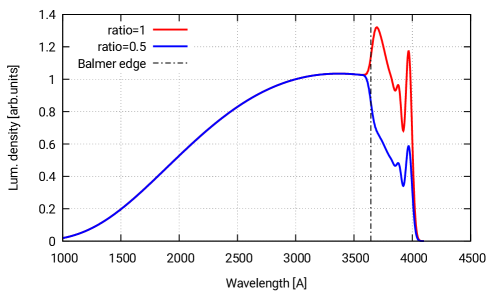
The whole component (sum of Balmer continuum and high order lines) is finally broadened by a Gaussian profile of 5000 km s-1. A plot of the Balmer template, for two values of the ratio of the high order blended line complex to the Balmer continuum (1 and 0.5 respectively) is shown in Fig. 1. The electron temperature and density, optical depth at Balmer edge and width of broadening profiles are fixed by default, but can be left free to vary for specific purposes. Also, for sources with we observe the spectrum at wavelengths shorter than 4000Å, i.e. we miss the most characterizing part of the Balmer continum. At 3500Å the Balmer continuum resembles a simple power law, and it would become degenerate with the continuum component. Therefore we fixed and = 0.3 for sources with (see Fig. 23).
2.4 Host galaxy
The host galaxy may contribute to the observed luminosity of an AGN, especially at optical/IR wavelengths. It is therefore necessary to disentangle its contribution from the AGN continuum to provide reliable estimates of the latter (e.g. Vestergaard et al., 2008). The galaxy spectra typically show a change of slope at 4000Å, corresponding to the Wien’s tail of black body spectra from stars, as shown in Fig. 2. This change of slope can be detected in SDSS spectra of low–luminosity, low redshift () AGN (e.g. Fig. 3 in Calderone et al. 2012) and can be used in automatic fitting procedures to estimate the host galaxy contribution.
In the current QSFit implementation we used a simulated 5 Gyr old elliptical galaxy template (Silva et al., 1998; Polletta et al., 2007) with a normalization factor as the only parameter.
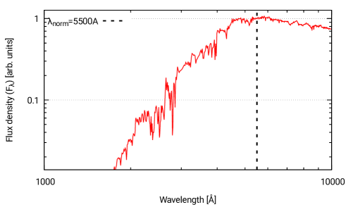
The template is normalized to have luminosity density of 1 at 5500Å, hence the value of the normalization parameter is the luminosity density of the host galaxy at 5500Å. We chose the elliptical template since luminous AGN (as those considered in the QSFIT catalog, §3) are likely hosted in elliptical galaxies (e.g. Floyd et al., 2004). For sources with we disabled the host galaxy component since the SDSS rest frame spectral range covers wavelengths shorter than 5000Å, providing weak constraints on the host galaxy component.
Our approach in fitting the host galaxy contribution with a single template is clearly simplistic, but it allowed us to homogeneously analyze a very large sample. More sophisticated AGN/host galaxy decomposition methods have been proposed by other authors (e.g. Barth et al., 2015; Matsuoka et al., 2015), and could in principle be used also with QSFit by customizing it for specific needs (§B).
2.5 Blended iron lines
Modeling of both broad and narrow (permitted and forbidden) iron lines is essential for a proper estimate of broad–band continuum and contaminated lines (such as Mg ii and H), especially if the source shows small widths of broad lines (Boroson & Green, 1992). In the current QSFit implementation we used the iron template of Vestergaard & Wilkes (2001) at UV wavelengths, and the iron template of Véron-Cetty et al. (2004) at optical wavelengths.
2.5.1 Iron emission lines at optical wavelengths
At optical wavelengths we used the spectral decomposition of I Zw 1 made by Véron-Cetty et al. (2004), spanning the wavelength range from 3500 to 7200Å (rest frame).
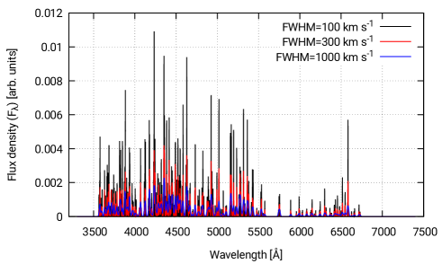
To compare the observed data with the optical iron template we prepared a grid of templates, each with its own value of FWHM. To generate each template we sum a Gaussian profile (of the given FWHM) for each line listed in tables A.1 and A.2 of Véron-Cetty et al. (2004) (excluding the hydrogen Balmer lines). The relative line intensities are fixed to those reported in the tables,111111We considered only the William Herschel Telescope (WHT) intensities and the final template is normalized to 1. Hence, the model parameters are the width of the lines (which identifies a template in our grid) and its overall normalization. The “broad” and “narrow” templates (tables A.1 and A.2 respectively) are kept separated, each with its own parameters. The FWHM in our grid vary from 103 to 104 km s-1 for the broad templates, and from 102 to 103 km s-1 for the narrow templates. A plot of the iron template, for three values of FWHM (103, 3 and 104 km s-1) is shown in Fig. 3.
The iron emission at optical wavelengths is typically weak, and the SDSS spectral resolution is not sufficient to provide robust constraints to the FWHM values, hence we keep it fixed at 3000 km s-1 for the broad component and to 500 km s-1 for the narrow component. These constraints can be relaxed when using data with higher spectral resolution.
2.5.2 Iron emission lines at UV wavelengths
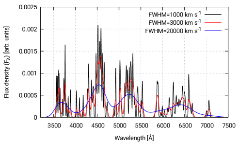
We considered the “B” template and the FeII UV191 and FeIII UV47 multiplets of the iron template described in Vestergaard & Wilkes (2001), spanning the wavelength range from 1250Å to 3090Å. The original template is based on the observations of I Zw 1, whose FWHM of broad lines is 900 km s-1. To adapt the template to sources with broader emission lines we prepared a grid of broadened templates by convolving the original one with a set of Gaussian profiles, whose FWHM range from 103 to 2 km s-1. In this case there is no separation between “broad” and “narrow” contributions since the original template in Vestergaard & Wilkes (2001) is the sum of both. A plot of the template, for three values of FWHM (103, 3 and km s-1) is shown in Fig. 4.
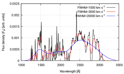
The model parameters are the equivalent width (integrated over the whole wavelength range 1250Å to 3090Å) and the FWHM of the profile used to broaden the template. The FWHM values are constrained in the range 103–104 km s-1. The SDSS spectral resolution is not sufficient to provide robust constraints to the FWHM value, hence we keep it fixed at 3000 km s-1. This constraint can be relaxed when using data with higher spectral resolution. Also, for sources with we fix the iron UV equivalent width to 138Å (i.e. the median of the values measured at larger redshifts) since only a small part of the whole template is visible, and the iron normalization would become degenerate with the continuum slope. Moreover fixing the UV iron helps in constraining the continuum slope to have similar distributions at redshifts below and above 0.4.
2.6 Main emission lines
The broad and narrow emission lines considered in QSFit are shown in Tab. 1. Each line is modeled with a Gaussian profile, whose fitting parameters are the total (integrated) line luminosity, the FWHM and velocity offset (with respect to the reference wavelength) of the line profile.
| Line | Wavelength [Å] | Type | Field name |
|---|---|---|---|
| Si iv | 1399.8 | B | br_siiv_1400 |
| C iv | 1549.48 | B | br_civ_1549 |
| C iii] | 1908.734 | B | br_ciii_1909 |
| Mg ii | 2799.117 | B | br_mgii_2798 |
| [Ne vi] | 3426.85 | N | na_nevi_3426 |
| [O ii] | 3729.875 | N | na_oii_3727 |
| [Ne iii] | 3869.81 | N | na_neiii_3869 |
| H | 4102.89 | B | br_hd |
| H | 4341.68 | B | br_hg |
| H | 4862.68 | B | br_hb |
| N | na_hb |
||
| [O iii] | 4960.295 | N | na_oiii_4959 |
| [O iii] | 5008.240 | N | na_oiii_5007 |
| He i | 5877.30 | B | br_hei_5876 |
| [N ii] | 6549.86 | N | na_nii_6549 |
| H | 6564.61 | B | br_ha |
| N | na_ha |
||
| (see text) | line_ha_base |
||
| [N ii] | 6585.27 | N | na_nii_6583 |
| [Si ii] | 6718.29 | N | na_sii_6716 |
| [Si ii] | 6732.67 | N | na_sii_6731 |
The FWHM of narrow and broad lines is constrained in the range [102, 2] km s-1 and [9, 1.5] km s-1 respectively. The velocity offset of narrow and broad lines is constrained in the range km s-1 and km s-1 respectively. For the H and H emission lines we used both a broad and narrow components, but we had to limit the FWHM of the narrow component to [102, ] km s-1 to allow a good decomposition of the line profile. Also, we had to limit the Mg ii broad component velocity offset to km s-1 to avoid degeneracies with the UV iron template. Finally, we used three components to fit the H to account for the very broad feature below that line. The FWHM of the H “base” line is constrained in the range [104, ] km s-1.
A line component is ignored if the resulting line profile would fall outside (even partially) the available wavelength range. Moreover, a line component is ignored if the amount of dropped spectral channels (whose quality mask is not 0, §2.8.1), in the wavelengths relevant to the emission line, exceeds 40%. These precautions were taken to ensure the emission line parameters can actually be constrained by the available data.
2.7 “Unknown” emission lines
Beyond the “known” emission lines (§2.6) expected to be relevant in any AGN, we also considered a list of 10 “unknown” emission lines, i.e. not a priori associated to any known line. These emission lines are added after all the other components (see §2.8), and their initial wavelength is set at the position where there is the maximum positive residual. By considering these further components we may account for the lack of an iron template in the wavelength range 3100–3500Å, or for asymmetric profiles in known emission lines.
2.8 Fitting procedure and data reduction
In this section we describe the spectral analysis procedure, which runs through four distinct steps: (i) preparation of the spectrum, (ii) model fitting, and (iii) data reduction.
2.8.1 Spectrum preparation
The current QSFit implementation operates only on spectra observed by the the Sloan Digital Sky Survey, data release 10 (SDSS–DR10, York et al., 2000; Ahn et al., 2014).
To prepare the spectrum we drop the 100 spectral channels at the beginning and end of each spectrum to avoid artifacts from instrument or pipeline. Then we drop the spectral channels whose quality mask is not equal to zero. If the remaining “good” channels accounts for less than 75% of the original channels, corresponding to 2700 channels, QSFit issues an error and skips the analysis. In the vast majority of cases the final wavelength range in the observer frame is 4150–8740Å, and the number of channels is 3450. The spectral resolution is 150 km s-1.
The spectrum is corrected for Galactic extinction using the CCM parametrization by Cardelli et al. (1989) and O’Donnell (1994), assuming a total selective extinction A(V) / E(B-V) = 3.1. We neglected any intrinsic (i.e. rest frame) reddening of the spectrum since most of sources show small or no reddening at all (e.g. Grupe et al., 2010). To build the QSFIT catalog (§3) we used the same color excess and redshift estimates as S11. Finally, the spectrum is transformed to the rest frame using the redshift estimate. The fitting process is performed by comparing the data and the model, in units of erg s-1 Å-1.
2.8.2 Model fitting
The fitting process occurs by varying the component parameters until the , as obtained by comparing the data and the model, is minimized. The minimization procedure follows a Levenberg–Marquardt algorithm, hence the result may depend significantly from the initial (guess) parameter values. In order to develop an “automatic” spectral analysis (without human intervention) we should find a proper way to get rid of such dependency on initial parameters. We found that a promising approach is to build the model step by step, i.e. by iteratively adding a component and re–running the minimization procedure.
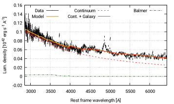
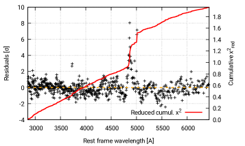
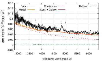
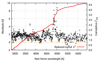
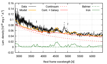
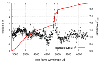
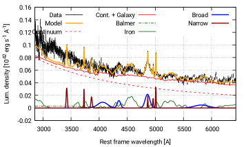
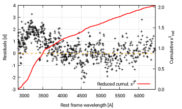
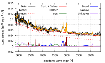
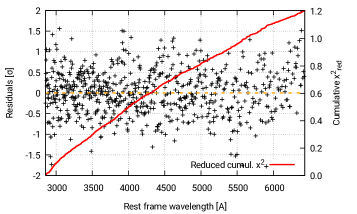
In the following we will discuss the five steps involved in the fitting process. The plots of data, model and residuals at each step of the fitting procedure are shown in Fig. 5. In order to produce clearer plots all data, as well as the model, were rebinned by a factor of 5. The analysis, however, has been carried out at full resolution. Additionally, the catalog browser web tools allows the user to view the data using any rebinning factor.
-
1.
The first components being added are the AGN continuum (actually a power law, §2.2) and the host galaxy template (§2.4). A first minimization is performed, which will bring the “best fit” model to pass through the data, without accounting for any emission line. The amount of positive residuals, calculated as (data model) / uncertainty, is approximately equal to the amount of negative residual.
-
2.
In order to provide room for further components (namely the emission lines) we lower the continuum normalization until the positive residuals reach %,121212Although there appear to be some arbitrariness in performing this step, we found that the final results (after all the remaining steps have been performed) depends weakly on the fraction of positive residuals, as long as the latter is above %. and fix all parameters of both AGN continuum and host galaxy components for the next iterations.
-
3.
We add the components for the iron templates at UV and optical wavelength (§2.5). The optical template is enabled for sources with , while the UV iron template is always enabled, although the equivalent width is fixed to 138Å if (§2.5.2). Then we re–run the fitting process by varying just the iron template parameters and we fix them at their best fit values for the next iterations.
-
4.
Now we add the “known” emission lines, and ensure there are enough spectral channels to constrain the line parameters, otherwise the line is ignored (§2.8.1). After re–running the minimization we fix all the emission line parameters for the next iterations.
-
5.
we iteratively add the “unknown” emission lines (§2.7), i.e. lines which are not a–priori associated to any specific transition. The center wavelength of these lines is first set at the position of the maximum positive residual, i.e. where most likely there is some further emission component, and then left free to change during the fitting process. We repeat this procedure up to 10 times. Finally we re–run the fitting process with all parameters, for all components, left free to vary. At the end we check which “unknown” line component is actually required to provide a better fit: if the line luminosity uncertainty is greater than 3 time the luminosity we disable the component and re–run the fit.
2.8.3 Data reduction
After the fitting process we use the resulting best fit parameter values to compile a list of spectral properties for the source being analyzed. In a few cases a further reduction is required to provide the final quantities. The details of the reduction process are as follows:
-
•
the AGN continuum and galaxy luminosities are estimated directly on the continuum component values, in at least six wavelengths, five of them equally spaced in the (logarithmic) wavelength range [+5%, %]. We restricted the range by 5% on both sides to avoid artifacts at the edges of the available spectrum. The other estimates are given at the fixed rest frame wavelengths 1450Å, 2245Å, 3000Å, 4210Å or 5100Å, depending on the source redshift;
-
•
the “unknown” lines are associated to the “known” emission lines if the center wavelength of the latter falls within the FWHM of the former. The association is performed only if the “unknown” line has a FWHM of at least 1000 km s-1 and the “known” line being considered is a broad line (narrow lines are always modeled with a single component). If two or more emission lines components are associated then we compute the total line profile as the sum of individual line profiles, and estimate the relevant quantities as follows:
-
–
the line luminosity is the sum of integrated luminosities of each component;
-
–
the FWHM is the full–width of the total profile at half the maximum of the total profile peak;
-
–
the velocity offset is calculated by considering the offset between the total profile peak position and the emission line reference wavelength;
The uncertainties on the luminosity is computed as the weighted sum of the luminosity uncertainty on each component. The uncertainties on FWHM and velocity offset are computed as the weighted average of the corresponding uncertainties in the fit parameters, with the weight given by the line intensities. These parameters are typically degenerate hence the uncertainties may be underestimated, see §B.4 for a different approach to estimate parameter uncertainties;
-
–
-
•
beyond the spectral quantities, we also provide several “quality flags” to assess the reliability of the automatic results. If a flag is raised for a given source then the corresponding quantity should be used cautiously, and a visual analysis of the spectrum is recommended. To produce the plots in the following sections we considered only the sources with no quality flag raised (i.e. whose quality flag is 0). The list of all quality flags and their meaning is discussed in §A, while the tables in §C summarize the fractions of sources which raised a quality flag.
All quantities calculated by QSFit are described in §A.
The uncertainties provided by QSFit are calculated using the Fisher matrix method (e.g. Heavens, 2009; Andrae, 2010), by assuming Gaussian uncertainties in the SDSS data, negligible correlation among model parameters, and symmetric uncertainty intervals. These assumptions are not always justifiable, hence QSFit uncertainties should be considered as rough estimates of parameter uncertainties. A better approach, although significantly more demanding in terms of computational time, is to use the Monte Carlo resampling method as discussed in §B.4. In the following we will always consider the Fisher matrix uncertainties provided by QSFit.
2.9 QSFit plots
After analyzing the data QSFit produces two plots using gnuplot.131313http://gnuplot.info/ An example is shown in Fig. 6: the upper panel shows the comparison between the SDSS data with their error bars (black vertical lines) and the QSFit model (orange line); the lower panel shows the residuals (data minus model) in unit of uncertainties in the data (black cross symbol) and the cumulative (red line, values on the right axis). The upper panel also shows the individual component in the QSFit model: the dashed red line is the continuum component (§2.2), while the solid red line is the sum of continuum and host galaxy components (§2.4); the dot–dashed green line is the Balmer component (§2.3); the solid green lines are the optical (§2.5.1) and UV (§2.5.2) iron templates; the sum of all broad and of all narrow emission line (§2.6) components are shown with blue and brown lines respectively. The sum of all “unknown” lines (§2.7) is shown with a purple solid line. The red squared and green circle symbols are the continuum luminosity estimated by QSFit and S11 respectively. The thick green line segments show the slopes estimated by S11 (anchored on the short wavelength side on QSFit continuum component).
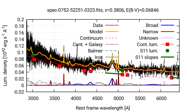
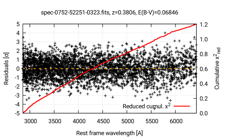
In the example shown in Fig. 6 the comparison between the data and the QSFit model yield a value of 1.19, with 3248 degrees of freedom (DOF). Given the very high number of DOF the probability of obtaining a worst by random fluctuations is very low (), hence the model should actually be rejected on a statistical basis. Nevertheless a qualitative inspection shows that the residuals are equally distributed on positive and negative values, and the cumulative line (red line in lower panel) do not shows significant “jumps” or discontinuities. Also, the spectral decomposition of the H and [O iii] region, as well as the iron emission, appear reasonable. Finally, the correlation among parameters (§B.4) implies that the actual number of DOF is larger than the quantity spectrum channel free parameters, hence the quoted is actually an upper limit for the actual value. In summary, we consider our spectral quantities reliable, even if the model should be rejected according to the goodness of fit test.
3 The QSFIT catalog
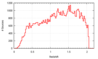
We used QSFit to analyze a subsample of the fifth edition of the SDSS quasar catalog Schneider et al. (2010), i.e. the same sample analyzed by Shen et al. (2011, the S11 catalog). We selected all the objects in the S11 catalog whose redshift is and whose BAL_FLAG is set to 0, i.e. they are not broad–absorption line quasars. This amounts to 79,986 sources. Then we dropped all the sources whose number of “good” spectral channels (quality mask=0) was less than 75% (§2.8). The final sample comprises 71,251 sources, which make up the QSFIT catalog (version 1.2) of spectral quantities. Fig. 7 shows the redshift distribution in our sample (upper panel) and the distribution of the SDSS flux density vs. its uncertainty (lower panel).
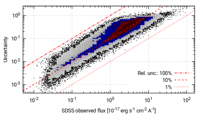
The colors in the 2–dimensional histogram in the lower panel of Fig. 7 represent the count densities. The bins drawn with a red and blue palette contain respectively 40% and 70% of the sources, the gray, red and blue ones (taken together) contain 95% of the sources. The remaining 5% are shown with individual dots. This color code is used for all the 2–D plots in this paper.
For each source in our subsample we performed the spectral analysis using the QSFit procedure and collected all the results in the QSFIT catalog. A similar work has already been done by Shen et al. (2011), although with a different approach (§4). In order to perform a meaningful comparison of our results and those from S11 (§4) we used exactly the same redshift and E(BV) values used by S11, as well as their cosmology ( km s-1 Mpc-1, and ).
In order to estimate the reliability of QSFit results we performed a qualitative visual inspection of many of the QSFit plots (§2.9) and found that our model usually provides a rather good representation of the data. A quantitative assessment of the agreement is given by the values, whose median value is 1.09 and is almost always smaller than 2 (Fig. 8, upper panel).
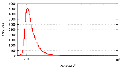
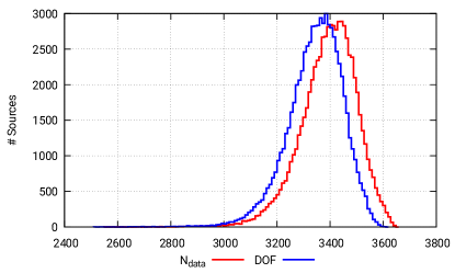
The number of DOF is typically in the range [3100, 3600] with a median value of 3380 (Fig. 8, lower panel). Despite the rather low values of the goodness of fit tests typically fails since the number of DOF is very high. Hence the QSFit model is too simple to account for all the details available in the data, and further components are likely required (e.g. emission lines, improved iron and host galaxy templates, etc.). Nevertheless, as discussed in (§2.9), a qualitative examination of the QSFit plots, as well as a comparison with the S11 catalog (§4), typically ensure that the spectral quantities can be considered reliable estimates. The “average” reliability of the QSFit estimates can also be assessed by comparing the average SDSS spectra with the average QSFit components (see Fig. 12 and the discussion in §5.2).
Moreover, the current QSFit implementation aims to provide a reasonably good fit of SDSS data in the vast majority of the cases. In order to provide a more accurate representation of the data, the QSFit procedure can be customized and tuned for the analysis of a specific source (§B).
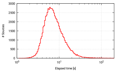
The QSFIT catalog is available as a FITS file141414http://qsfit.inaf.it/cat_1.2/fits/qsfit_1.2.fits where we report all the columns discussed in §2.8.3, as well as all the columns from the S11 catalog. The QSFIT catalog is also browsable through a web tool151515http://qsfit.inaf.it/ which allows the user to search for a specific source, sort sources according to a parameter, e.g. redshift, interactively browse the spectra inspecting the various model components, eventually rebinning the spectra, and finally download the plots (comparison of data and model, fit residuals) and the QSFit log file for a specific source. The rather low computational time ( 7 seconds on a modern day laptop, Fig. 9) required to analyze a source allows to re–run the analysis of individual source, re–build the whole QSFIT catalog, expand it, etc., without the need for expensive computational resources.
4 Comparison of S11 and QSFIT catalogs
In this section we will compare our results with those from Shen et al. (2011, S11) in order to assess the reliability of QSFit results. Although the purpose of both the S11 and QSFIT catalogs is similar, the adopted analysis algorithms show significant differences. The most relevant are:
-
•
S11 evaluates the continuum underlying the emission lines over a rather narrow wavelength range, in the neighborhood of the line, whereas QSFit uses a continuum component spanning the whole available wavelength range (§2.2);
-
•
S11 fits the continuum and iron contributions first, then subtract them from the observed flux, and finally fits the emission lines. QSFit follows a similar approach, but at the last step all parameters (continuum + galaxy + iron + emission lines) are free to vary simultaneously;
-
•
S11 neglects the host galaxy contamination while QSFit uses an elliptical galaxy template to account for such contribution (§2.4);
- •
-
•
S11 models the broad emission lines with either one, two or three Gaussian profiles, according to which case provide the best fit. Also, the [O iii]4959Å and [O iii]5007Å are both modeled with two Gaussian profiles. QSFit always starts with a single Gaussian profile for each broad and narrow line. If an “unknown” emission line (§2.7) lies sufficiently close to a “known” line it can be associated to the latter (§2.8.2) and the final profile may be modeled with more than one Gaussian profile. Tab. 5 shows how many lines were fitted with more than one component.
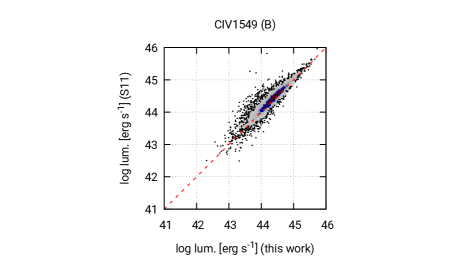
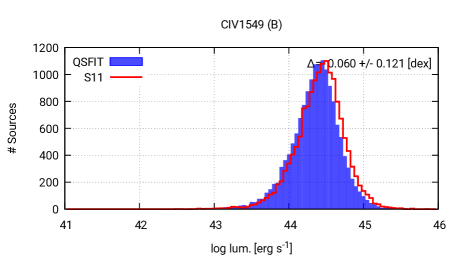
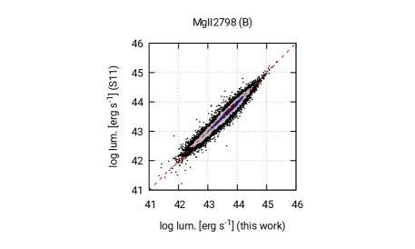
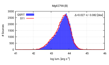
Despite the differences in the adopted analysis algorithms, in several cases the spectral estimates in the S11 and QSFIT catalogs show a very good correlation, as is the case for, e.g., the continuum luminosity estimates and the C iv 1549Å, Mg ii 2798Å and H 4861Å emission line luminosities.
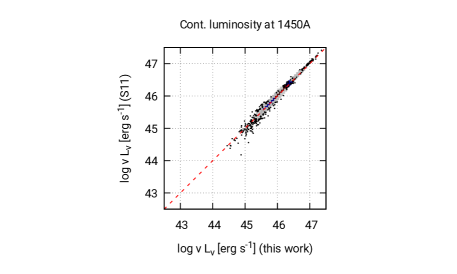
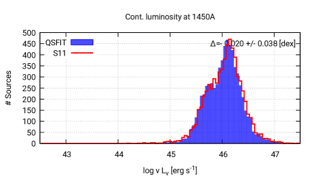
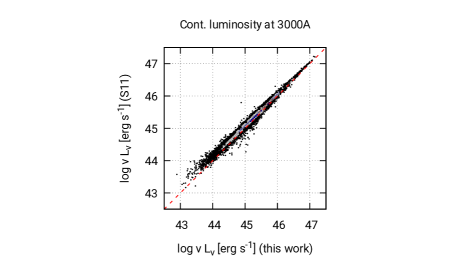
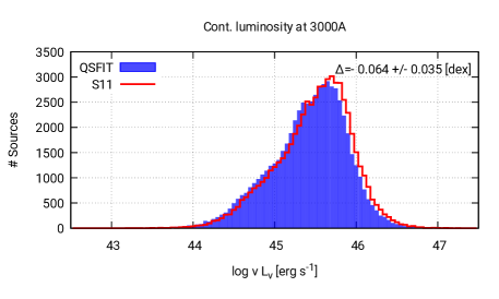
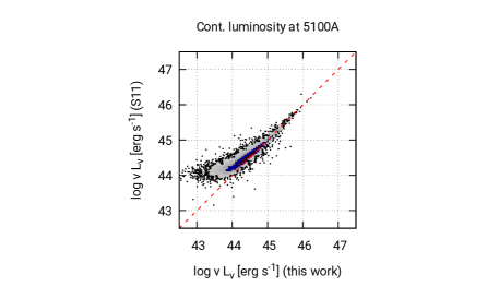
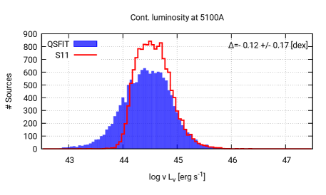
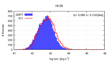
Fig. 10 shows the comparison of QSFit and S11 continuum luminosity estimates at 1350Å, 3000Å and 5100Å. The left panels show the 2–D histogram plots (see §3 for a description of such plots) with QSFit values on the X axis and S11 values on the Y axis (the red dashed line is the equality line). The right panels show the comparisons between the population distributions. The average and standard deviation of the difference between the two catalogs is shown in the upper right corner. The estimates are compatible in the two catalogs with a scatter of 0.04 dex (10%) over 2 dex, except for the 5100Å case of low luminosity AGN ( erg s-1) since the host galaxy contribution has been considered in QSFit but neglected in S11 (see also §5.2).
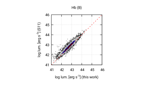
Fig. 11 shows the same comparisons for the broad component luminosities of C iv 1549Å, Mg ii 2798Å and H 4861Å emission lines: also in this case the correlation is quite good, although the scattering is larger ( dex %) over dex. The most prominent differences are in the C iv 1549Å and H 4861Å emission lines, and are mainly due to the different continuum assumed below the lines (§2.8). In QSFit such continuum is the sum of all the components except the “known” emission lines.
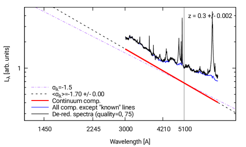
The reliability of such continuum can be inferred, at least on average, by comparing the averaged SDSS de–reddened spectra (in a narrow redshift bin) with the averaged sum of all QSFit components except the “known” emission lines. Such comparison is shown in Fig. 12, with the averaged spectrum of SDSS de–reddened spectra in the redshift bin shown with a black line, and the average spectrum of the sum of all QSFit components except the “known” emission lines shown with a blue line. The agreement between the blue and black lines is remarkably good over the entire wavelength range (except the regions of the main emission line). Hence the blue line represent a reliable estimate of the continuum below the line (at least on average). The averaged (or composite) spectra are further discussed in §5.2.
The very good agreement in continuum and emission line luminosities, spanning 2 dex, stem from both an accurate spectral analysis, and the relatively large redshift range considered. Indeed, when considering quantities which do not depend directly on redshift the correlation is worse, although still present. This is the case for, e.g., the continuum slopes (Fig. 13) and the emission line widths (Fig. 14).
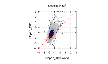
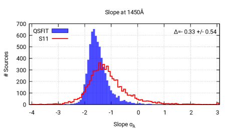
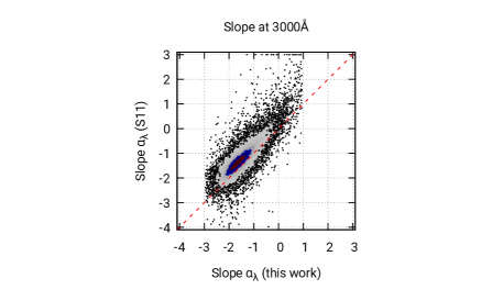
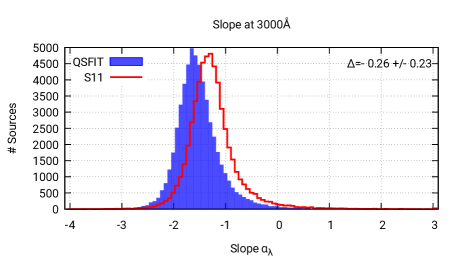
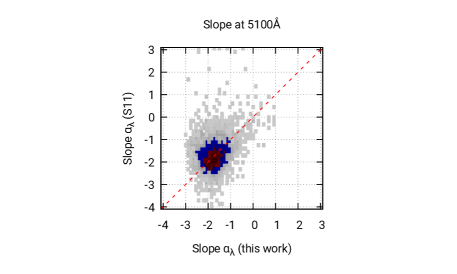
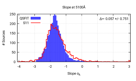
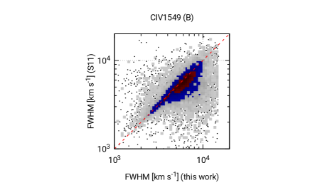
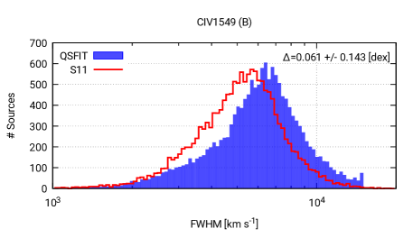
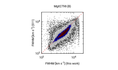
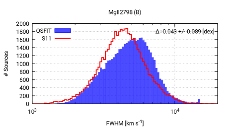
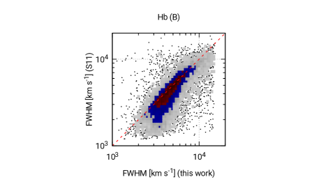
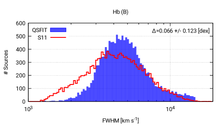
The discrepancies are mainly due to the different adopted algorithms. For instance, in the case of continuum slopes, we refer to the broad band continuum slopes, while S11 refer to the local continuum in the neighborhood of an emission line.161616The plots available in the QSFit web page allow for a quick comparison of the spectral slopes of both the QSFIT and S11 catalogs. Moreover, the emission line widths show a significant scattering ( dex, %, over less than 1 dex) since the line profile decomposition algorithm is very different. These findings show that estimating the emission line widths is not a an easy and straightforward task, and the availability of a commonly accepted procedure would be very useful.
The rather low average differences between the populations of luminosities and line widths discussed above allow us to conclude that, at least on average, the QSFit estimates are as reliable as the S11 ones. Since there is not yet a complete understanding of the emission processes generating the broad band continuum or the emission lines, there is not a clear way to prefer either the S11, QSFit, or any other catalog. The advantage in using the QSFit one is simply that the analysis is performed in an automatic (i.e. fast on large data sets), replicable and shareable way. Moreover it allows users to customize and fine tune the analysis for specific sources.
5 Discussion
The main purpose of the QSFIT catalog is to analyze the average spectral properties of Type 1 AGNs by taking advantages of the large SDSS dataset, instead of focusing on individual sources whose spectrum may be affected by low signal to noise ratio, or be peculiar in some aspect. A thorough analysis of the QSFIT results is, however, beyond the purpose of this work, and will be discussed in forthcoming papers. Here we will briefly explore the QSFIT data to check whether they follow the empirical relations already known in literature (§5.1), discuss the reliability of the QSFit continuum slope estimates (§5.2) and present a few of the major results (§5.3).
5.1 Empirical relations
Several empirical relations have been identified among AGN spectral quantities (e.g. Sulentic et al., 2000). One of the most important ones is the “Baldwin effect” (Baldwin, 1977), i.e. the correlation between the C iv1549Å equivalent width and the continuum luminosity.
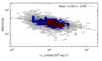
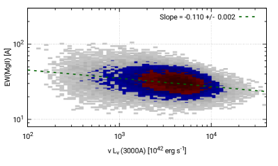
As new data became available similar correlations have been found for other emission lines (e.g. Baldwin et al., 1989; Kinney et al., 1990; Pogge & Peterson, 1992; Green et al., 2001). In Fig. 15 we show the Baldwin effect for the C iv 1549Å (upper panel) and Mg ii 2798Å emission lines (lower panel) using the data from the QSFIT catalog. The slopes (shown in the upper right corner of the plots) are very similar to those reported in Green et al. (2001), and for C iv 1549Å and Mg ii 2798Å respectively, although the sample used here is significantly larger.
Another important set of correlations has been highlighted by means of the Principal Component Analysis (PCA). The spectral quantities which build up the “Eigenvector 1” (i.e. the main driver for the variance in the observed spectral properties Boroson & Green, 1992) are the peak luminosity ratios between [O iii] and H, the equivalent width of the [Fe ii] complex at optical wavelengths, the width of the H emission line and a few others. These quantities present strong correlations, which are likely the manifestation of the underlying AGN physics (e.g. Wang et al., 1996; Boroson, 2002; Sulentic et al., 2003). In Fig. 16 we show two such correlations between the width of the broad H emission line (upper panel) and the peak luminosity ratios between [O iii] and H (lower panel) vs. the [Fe ii] equivalent width, using the data from the QSFIT catalog.
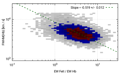
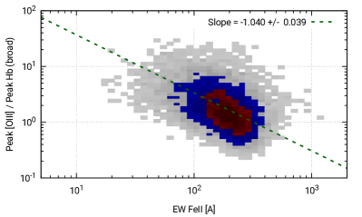
These examples show that the data in the QSFIT catalog allow to recover the most common empirical relations known in literature. By exploiting the very large QSFIT catalog and its additional estimates not previously available (such as the AGN continuum slopes or the host galaxy luminosities) it will be possible to study in a much deeper detail the correlations. These topics will be the subject of a forthcoming paper.
5.2 Reliability of continuum slope estimates
In order to assess the reliability of QSFit continuum estimates we compared the SDSS de–reddened averaged (or composite) spectrum with the average spectrum of the QSFit continuum components in a few subsamples spanning a very narrow redshift range. Each composite spectrum is calculated as the geometrical average of all spectra in the subsample, in order to preserve the slopes in a log–log plot. Before calculating the average we normalize each de–reddened spectrum and the associated QSFit components by the source luminosity at wavelength . Fig. 17 shows such a comparison for the sources in the redshift bins , , and respectively, using Å (vertical grey line). The redshift bins are shown in the upper right corner. The bin at is larger in order to contain a sufficient number of sources.
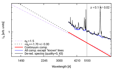
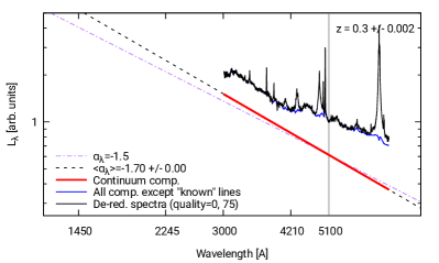
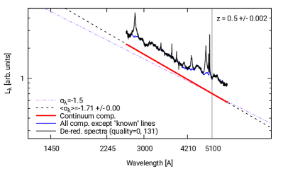
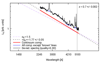
The composite spectrum of the sources in the redshift bin whose continuum quality flag at is 0 (CONT5100__QUALITY, §A) is shown with a black solid line. The number of sources in this subsample is shown in the legend. Also shown are the composite spectrum of the QSFit continuum component alone (shown with a red line) and the composite spectrum obtained by summing all the QSFit components except the “known” emission lines (blue line). The latter represents the “floor” below the emission lines, i.e. the sum of the AGN, host galaxy, iron complex and Balmer continuum contributions as estimated by QSFit. The average QSFit slope at is shown with a (black dashed line), and the numerical value is shown in the legend along with the associated standard deviation of the mean. Finally the purple dot–dashed line identifies the reference slope , to be discussed below. A similar comparison is shown in Fig. 18 for the sources at , , and respectively, using Å.
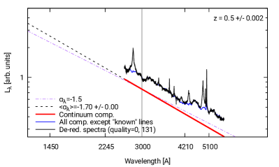
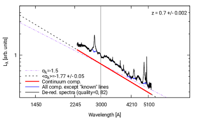
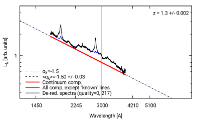
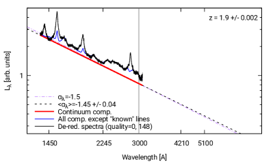
In all plots the blue line follows accurately the black line.171717Such agreement between the blue and black line is best visible when the arithmetic average is used, like in Fig. 12, in place of the geometric one. However, in this section the focus is on the reliability of the slopes hence we decided to show the geometric composites only. The plots with both geometric and arithmetic composites in all the redshift bins between 0.1 and 2 are available in the QSFit webpage. Hence QSFit is able to find the appropriate continuum below the main emission lines, and the host galaxy, Balmer continuum and iron templates appear adequate to fit the SDSS spectra. Having considered such components in the above discussion, the remaining contribution is what we assumed to be the AGN continuum (§2.2), whose composite spectrum is shown with the red line, and whose average slope is shown with a black dashed line.
5.3 QSFIT catalog main results
Here we will discuss two of the most important results of the QSFit analysis, namely the lack of appreciable redshift evolution of the AGN continuum slope and of the Balmer continuum luminosity (when normalized with continuum luminosity).
In Fig. 19 we show the ratio of galaxy luminosity over continuum luminosity, both estimated at 5100Å, as a function of redshift. At redshifts the AGN continuum component contribution is smaller than, or comparable with, the emission from the galaxy (Fig. 19).
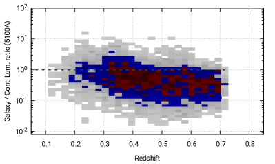
This explains why our continuum luminosity estimates are smaller than the S11 ones (see Fig. 10) at low luminosities. However, for these sources we can only indirectly probe the AGN continuum, and our estimates rely on the assumptions that the host galaxy template and the fixed continuum slope ( for the sources with , §2.2) are suitable for the source being analyzed. Hence, the QSFit continuum properties (especially the slopes) for sources with may be biased by our assumptions. At redshifts the galaxy contribution become gradually less important and the AGN continuum can in principle be directly probed. However, the presence of a very broad emission feature between 2200Å and 4000Å known as “small blue bump” (SBB, due to the Balmer continuum and many blended iron lines, Wills et al., 1985), clearly visible in the lower left panel of Fig. 18, may introduce a bias in the QSFit slope estimates. The bias is due to the fact that at the small blue bump is not entirely visible using just the data at optical wavelengths, and consequently the AGN continuum component is “pulled upward” at short wavelengths to fit the regions close to the Mg ii emission line. The slope would be, therefore, systematically underestimated. As a consequence we had to fix the continuum slope for the sources with . In order to remove this limit additional data at UV wavelengths are required.
At redshifts the small blue bump is almost always entirely visible (see Fig. 18, upper right panel) and the host galaxy is typically negligible, hence the QSFit slope estimates are not affected by the aforementioned bias, and the slope parameter is free to vary in the fit.
The 2–D histograms of slope vs. redshift for all sources whose
CONT*__QUALITY is 0 (§A) at the fixed
rest frame wavelengths 1450Å, 2245Å, 3000Å, 4210Å and
5100Å is shown in Fig. 20 (the meaning of the 2–D
histogram color code is described in §3). The dashed
red lines is at .
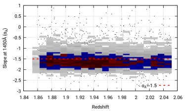
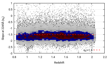
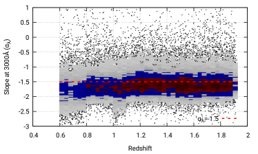
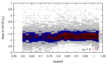
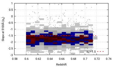
Fig. 21 shows the same data, but considering only the sources in very narrow redshift bins ().
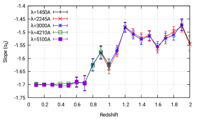
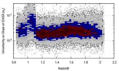
The slopes span the very narrow range between 1.45 and 1.65 at all redshifts between 0.8 and 2, providing remarkable evidence for the similarity of continuum slopes across cosmic time. This is in agreement with previous works: the typical value of the spectral slope at optical/UV wavelengths is (e.g. Richards et al., 2006; Vanden Berk et al., 2001; Shankar et al., 2016), however our analysis allows for the first time to estimate the slopes on a very large sample, using a completely automatic procedure and just the SDSS data at optical wavelengths. In particular, our estimates are similar to those of Davis et al. (2007), who found (in the wavelength range 1450–2200Å) and (in the wavelength range 2200–4000Å) with rather broad distributions (see their Fig. 2). At the slopes are remarkably constant and show no trend with redshift up to . The scatter is larger than the standard deviation of the mean in the redshift bins, hence the values are affected by small () slope systematics due to the fact that at different redshift we observe different parts of the rest frame spectrum. Moreover, note that the typical uncertainty associated to our estimates of ranges between 0.02 and 0.1 (Fig. 22), while the widths in the distributions of Fig. 20 are significantly larger (). Hence these distributions are not significantly broadened by the random uncertainties in the fitting process. We conclude that the average continue slope is , but there are AGNs whose slope is significantly smaller or larger than the average.
At the slopes are slightly smaller. Currently we are not able to discriminate whether the SBB bias is the only cause of such low slope estimates, or rather if the slopes actually are smaller at with respect to higher redshifts. Note that both the putative galaxy bias and the systematic SBB bias are not due to limitations of QSFit: they are a consequence of having considered just the spectra at optical wavelengths rather than considering data at shorter wavelengths. By enlarging the spectral coverage we could get rid of such biases and provide stronger constraints on the actual continuum shape at . On the other hand using just the SDSS data allowed us to analyze a very large and homogeneous sample.
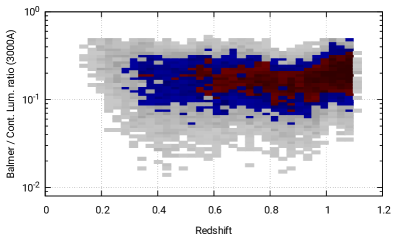
Similar conclusions applies to the ratio of the Balmer luminosity over the AGN continuum luminosity, both estimated at 3000Å. Fig. 23 shows distribution of the Balmer continuum normalization parameter (§2.3) in the upper panel, and the distribution as a function of redshift in the lower panel. The distribution is quite flat at all redshifts and has a median value of 0.15 and a width of 0.3 dex.

6 Conclusions
We presented QSFit (version 1.2), an IDL package able to automatically analyze the SDSS optical spectra of Type 1 AGNs. QSFit is released as free software, and can be customized to analyze the spectra from other sources, or to customize the fitting recipe. QSFit provides luminosity estimates for the AGN continuum, the Balmer continuum, both optical and UV iron blended complex, host galaxy and emission lines, as well as width, velocity offset and equivalent width of 20 emission lines, as well as several “quality flags” to assess the reliability of the results.
We used QSFit to analyze 71,251 SDSS spectra of Type 1 AGN at and to produce a publicly available catalog of AGN spectral properties (available on the QSFit website, along with additional data and plots). Also, we compared our results with those from the S11 catalog (Shen et al., 2011). The quantities are in very good agreement, except for: (i) the continuum luminosity at 5100Å for sources at low redshift, where we also considered the host galaxy contribution; (ii) the emission line widths whose values depend on the adopted fitting algorithm for line decomposition.
We also checked the reliability of the QSFit continuum slope estimates by a comparison with composite spectra of the observed SDSS data, and found that QSFit performs particularly well at , providing (for the first time) the AGN continuum slope estimates on a very large sample, using just the data at optical wavelengths and a completely automatic procedure. Also, we have shown that the continuum slope and the Balmer continuum luminosity distributions do not show any evident trend with redshift.
The release of the QSFit code and the associated catalog discussed in this work are the first attempt towards a new approach in analyzing AGN spectral data, where all interested astronomers are given the possibility to study and compare the analysis methods, easily replicate the data analysis (even on very large samples), and possibly improve the recipes in a collaborative effort.
ACKNOWLEDGEMENTS
We gratefully acknowledge our referee, Yue Shen, for useful suggestions and comments that greatly improved the presentation of this work.
We acknowledge M. Vestergaard and B.J. Wilkes for having provided the UV iron templates, and M.-P. Véron-Cetty, M. Joly and P. Véron for the optical iron templates used in the fitting process.
We warmly thank a number of undergraduate students at the University of Southampton who have widely tested QSFit on thousands of different sources and under different input assumptions.
We also thank Chiara Moretti for her contribution to the development of the QSFit website, and Guido Cupani for insightful discussions on fitting algorithms.
Funding for the SDSS and SDSS-II has been provided by the Alfred P. Sloan Foundation, the Participating Institutions, the National Science Foundation, the U.S. Department of Energy, the National Aeronautics and Space Administration, the Japanese Monbukagakusho, the Max Planck Society, and the Higher Education Funding Council for England. The SDSS Web Site is http://www.sdss.org/.
The SDSS is managed by the Astrophysical Research Consortium for the Participating Institutions. The Participating Institutions are the American Museum of Natural History, Astrophysical Institute Potsdam, University of Basel, University of Cambridge, Case Western Reserve University, University of Chicago, Drexel University, Fermilab, the Institute for Advanced Study, the Japan Participation Group, Johns Hopkins University, the Joint Institute for Nuclear Astrophysics, the Kavli Institute for Particle Astrophysics and Cosmology, the Korean Scientist Group, the Chinese Academy of Sciences (LAMOST), Los Alamos National Laboratory, the Max-Planck-Institute for Astronomy (MPIA), the Max-Planck-Institute for Astrophysics (MPA), New Mexico State University, Ohio State University, University of Pittsburgh, University of Portsmouth, Princeton University, the United States Naval Observatory, and the University of Washington.
References
- Ahn et al. (2014) Ahn C. P., Alexandroff R., Allende Prieto C., Anders F., Anderson S. F., Anderton T., Andrews B. H., Aubourg É., Bailey S., Bastien F. A., et al. 2014, ApJS, 211, 17
- Andrae (2010) Andrae R., 2010, (arXiv:1009.2755)
- Baldwin (1977) Baldwin J. A., 1977, ApJ, 214, 679
- Baldwin et al. (1989) Baldwin J. A., Wampler E. J., Gaskell C. M., 1989, ApJ, 338, 630
- Barth et al. (2015) Barth A. J., et al., 2015, ApJS, 217, 26
- Boroson (2002) Boroson T. A., 2002, ApJ, 565, 78
- Boroson & Green (1992) Boroson T. A., Green R. F., 1992, ApJS, 80, 109
- Burtscher et al. (2009) Burtscher L., Jaffe W., Raban D., Meisenheimer K., Tristram K. R. W., Röttgering H., 2009, ApJ, 705, L53
- Calderone et al. (2012) Calderone G., Sbarrato T., Ghisellini G., 2012, MNRAS, 425, L41
- Calistro Rivera et al. (2016) Calistro Rivera G., Lusso E., Hennawi J. F., Hogg D. W., 2016, arXiv:1606.05648
- Cardelli et al. (1989) Cardelli J. A., Clayton G. C., Mathis J. S., 1989, ApJ, 345, 245
- Cristiani & Vio (1990) Cristiani S., Vio R., 1990, A&A, 227, 385
- Davis et al. (2007) Davis S. W., Woo J.-H., Blaes O. M., 2007, ApJ, 668, 682
- Dietrich et al. (2002) Dietrich M., Appenzeller I., Vestergaard M., Wagner S. J., 2002, ApJ, 564, 581
- Elvis et al. (1994) Elvis M., et al., 1994, ApJS, 95, 1
- Floyd et al. (2004) Floyd D. J. E., Kukula M. J., Dunlop J. S., McLure R. J., Miller L., Percival W. J., Baum S. A., O’Dea C. P., 2004, MNRAS, 355, 196
- Francis et al. (1991) Francis P. J., Hewett P. C., Foltz C. B., Chaffee F. H., Weymann R. J., Morris S. L., 1991, ApJ, 373, 465
- Grandi (1982) Grandi S. A., 1982, ApJ, 255, 25
- Green et al. (2001) Green P. J., Forster K., Kuraszkiewicz J., 2001, ApJ, 556, 727
- Grupe et al. (2010) Grupe D., Komossa S., Leighly K. M., Page K. L., 2010, ApJS, 187, 64
- Heavens (2009) Heavens A., 2009, (arXiv:0906.0664)
- Kellermann et al. (1989) Kellermann K., Sramek R., Schmidt M., Shaffer D. B., Green R., 1989, AJ, 98, 1195
- Khachikian & Weedman (1974) Khachikian E. Y., Weedman D. W., 1974, ApJ, 192, 581
- Kinney et al. (1990) Kinney A. L., Rivolo A. R., Koratkar A. P., 1990, ApJ, 357, 338
- Kriss (1994) Kriss G., 1994, in Crabtree D. R., Hanisch R. J., Barnes J., eds, Astronomical Data Analysis Software and Systems III Vol. 61 of Astronomical Society of the Pacific Conference Series, Fitting Models to UV and Optical Spectral Data. p. 437
- Markwardt (2009) Markwardt C. B., 2009, in Bohlender D. A., Durand D., Dowler P., eds, Astronomical Data Analysis Software and Systems XVIII Vol. 411 of Astronomical Society of the Pacific Conference Series, Non-linear Least-squares Fitting in IDL with MPFIT. p. 251
- Matsuoka et al. (2015) Matsuoka Y., Strauss M. A., Shen Y., Brandt W. N., Greene J. E., Ho L. C., Schneider D. P., Sun M., Trump J. R., 2015, ApJ, 811, 91
- O’Donnell (1994) O’Donnell J. E., 1994, ApJ, 422, 158
- Pogge & Peterson (1992) Pogge R. W., Peterson B. M., 1992, AJ, 103, 1084
- Polletta et al. (2007) Polletta M., et al., 2007, ApJ, 663, 81
- Richards et al. (2006) Richards G. T., et al., 2006, ApJS, 166, 470
- Sanders et al. (1989) Sanders D. B., Phinney E. S., Neugebauer G., Soifer B. T., Matthews K., 1989, ApJ, 347, 29
- Schneider et al. (2010) Schneider D. P., et al., 2010, AJ, 139, 2360
- Shankar et al. (2016) Shankar F., et al., 2016, ApJ, 818, L1
- Shen et al. (2011) Shen Y., et al., 2011, ApJS, 194, 45
- Shen & Liu (2012) Shen Y., Liu X., 2012, ApJ, 753, 125
- Silva et al. (1998) Silva L., Granato G. L., Bressan A., Danese L., 1998, ApJ, 509, 103
- Storey & Hummer (1995) Storey P. J., Hummer D. G., 1995, MNRAS, 272, 41
- Sulentic et al. (2000) Sulentic J. W., Marziani P., Dultzin-Hacyan D., 2000, ARA&A, 38, 521
- Sulentic et al. (2003) Sulentic J. W., Zamfir S., Marziani P., Bachev R., Calvani M., Dultzin-Hacyan D., 2003, ApJ, 597, L17
- Telfer et al. (2002) Telfer R. C., Zheng W., Kriss G. A., Davidsen A. F., 2002, ApJ, 565, 773
- Urry & Padovani (1995) Urry C. M., Padovani P., 1995, PASP, 107, 803
- Vanden Berk et al. (2001) Vanden Berk D. E., et al., 2001, AJ, 122, 549
- Véron-Cetty et al. (2004) Véron-Cetty M.-P., Joly M., Véron P., 2004, A&A, 417, 515
- Vestergaard et al. (2008) Vestergaard M., Fan X., Tremonti C. A., Osmer P. S., Richards G. T., 2008, ApJ, 674, L1
- Vestergaard & Wilkes (2001) Vestergaard M., Wilkes B. J., 2001, ApJS, 134, 1
- Wang et al. (1996) Wang T., Brinkmann W., Bergeron J., 1996, A&A, 309, 81
- Wills et al. (1985) Wills B. J., Netzer H., Wills D., 1985, ApJ, 288, 94
- York et al. (2000) York D. G., et al., 2000, AJ, 120, 1579
Appendix A Description of the QSFIT catalog
The QSFIT (version 1.2) catalog is deployed as a FITS table with 279 columns and 71,251 rows, available at the following address:
http://qsfit.inaf.it/cat_1.0/fits/qsfit_1.0.fits
On the QSFit website you will also find a second version of the catalog where we added, for each analyzed source, the corresponding data from the S11 catalog to allow an easy comparison. This latter FITS file has 434 columns.
In this section we will list the name and meaning of each column in
the QSFIT catalog. The columns whose name has a
__QUALITY suffix require a preliminary explanation: they store
the “quality flags”, whose purpose is to characterize the
reliability of the associated quantity. If a quality flag is raised
for a given source then the corresponding quantity should be used
cautiously, and a further analysis is typically required. To save
space in the final catalog these flags are coded as “bits”,
i.e. quantities which can be either 0 (flag not raised) or 1 (flag
raised), and packed into a binary representation of an integer number
(the bitmask). For instance, a quality flag equal to 13 means that
the bits 0, 2, 3 are raised, since . A quality
flag equal to 0 means that no flag has been raised and the associated
quantity is considered reliable (within the capabilities of QSFit).
The meaning of each bit in the quality flag is discussed below.
The list of columns provided in the QSFIT catalog is:
-
•
SPEC: name of the SDSS–DR10 FITS file containing the spectrum; -
•
SDSS_NAME: the SDSS name of the source (J2000.0); -
•
RA: the right ascension (J2000.0) of the source; -
•
DEC: the declination (J2000.0) of the source; -
•
REDSHIFT: the redshift of the source -
•
PLATE: spectroscopic plate number; -
•
FIBER: spectroscopic fiber number; -
•
MJD: Modified Julian Day of spectroscopic observation; -
•
E_BV: the color excess used to de–redden the SDSS spectrum; -
•
NDATA: the number of channels in the spectrum used in the analysis (§2.8.1); -
•
GOOD_FRACTION: the fraction of “good” channels (whose SDSS mask is 0) over the total number of channels. This quantity is 0.75 for all sources analyzed in this work (§2.8.1); -
•
MEDIAN_FLUX, MEDIAN_ERR: the median flux and median uncertainty in the input spectrum, in units of 10-17 erg s-1 cm-2 Å-1; -
•
GALAXY__LUM, GALAXY__LUM_ERR: the host galaxy luminosity at 5500Å and its uncertainty, in units of erg s-1 (§2.4); -
•
GALAXY__QUALITY: quality flag for the galaxy estimates. The meaning of the bits are:-
–
Bit 0: fit of galaxy template is not sensible at this redshift;
-
–
Bit 1: either the luminosity or its uncertainty are NaN or equal to zero;
-
–
Bit 2: luminosity relative uncertainty 1.5;
-
–
-
•
CONT*__WAVEwhere “*” is a number in the range 1–5: wavelengths in Å where the continuum luminosity and slopes (see below) has been computed. There are five such quantities whose values are equally spaced in the logarithmic wavelength range [, ]; -
•
CONT*__LUM,CONT*__LUM_ERRwhere “*” is in the range 1–5, or equal to 1450, 2245, 3000, 4210 or 5100: AGN continuum (§2.2) luminosities and their uncertainties, in units of erg s-1, estimated at wavelengthsCONT*__WAVEor at the fixed rest frame wavelengths 1450Å, 2245Å, 3000Å, 4210Å or 5100Å; -
•
CONT*__SLOPE,CONT*__SLOPE_errwhere “*” is in the range 1–5, or equal to 1450, 2245, 3000, 4210 or 5100: AGN continuum slopes and their uncertainties estimated at wavelengthsCONT*__WAVEor at the fixed rest frame wavelengths 1450Å, 2245Å, 3000Å, 4210Å or 5100Å. The slopes are calculated as the derivative of the continuum component in the – plane, this approach allows to consider the most general case of the continuum modeled as a smoothly broken power law (§B.5). All the uncertainties are identical since they are given by the uncertainties of the and parameters of the AGN continuum component §2.2. Note that for sources with theCONT*__SLOPEis always and theCONT*__SLOPE_erris always 0; -
•
CONT*__GALAXYwhere “*” is in the range 1–5, or equal to 1450, 2245, 3000, 4210 or 5100: host galaxy luminosities, in units of erg s-1, estimated at wavelengthsCONT*__WAVEor at the fixed rest frame wavelengths 1450Å, 2245Å, 3000Å, 4210Å or 5100Å. These quantities are provided for a quick comparison with the AGN continuum luminosities. The relative uncertainty ofCONT*__GALAXYcan be estimated asGALAXY__LUM_ERR / GALAXY__LUM; -
•
CONT*__QUALITYwhere “*” is in the range 1–5, or equal to 1450, 2245, 3000, 4210 or 5100: quality flag for the AGN continuum estimates. The meaning of the bits are:-
–
Bit 0: wavelength is outside the observed range;
-
–
Bit 1: either the luminosity or its uncertainty are NaN or equal to zero;
-
–
Bit 2: luminosity relative uncertainty 1.5;
-
–
Bit 3: either the slope or its uncertainty are NaN or equal to zero;
-
–
Bit 4: slope hits a limit in the fit;
-
–
Bit 5: slope uncertainty 0.3;
-
–
-
•
IRONUV__LUM,IRONUV__LUM_ERR: the integrated luminosity and its uncertainty for the iron template at UV wavelengths, in units of erg s-1 (§2.5.2); -
•
IRONUV__FWHM,IRONUV__FWHM_ERR: the FWHM and its uncertainty of the Gaussian profile used to broaden the template, in units of km s-1. The SDSS data do not allow to reliably constrain this quantity, henceIRONUV__FWHMis always 3000 km s-1 andIRONUV__FWHM_ERRis always 0; -
•
IRONUV__EW,IRONUV__EW_ERR: the equivalent width and its uncertainty for the iron template at UV wavelengths, in units of Å; -
•
IRONUV__QUALITY: quality flag for the UV iron template. The meaning of the bits are:-
–
Bit 0: fit of iron template is not sensible at this redshift;
-
–
Bit 1: either the luminosity or its uncertainty are NaN or equal to zero;
-
–
Bit 2: luminosity relative uncertainty 1.5;
-
–
-
•
IRONOPT_BR__LUM,IRONOPT_BR__LUM_ERR: the integrated luminosity and its uncertainty for the “broad” iron template at optical wavelengths, in units of erg s-1 (§2.5.1); -
•
IRONOPT_BR__FWHM,IRONOPT_BR__FWHM_ERR: the FWHM and its uncertainty of the Gaussian profile used to build the template, in units of km s-1. The SDSS data do not allow to reliably constrain this quantity, henceIRONOPT_BR__FWHMis always 3000 km s-1 andIRONOPT_BR__FWHM_ERRis always 0; -
•
IRONOPT_BR__UNK_COUNT: number of “unknown” components (§2.7) whose center lies in the range 4460–4680Å or 5150–5520Å. i.e. which overlaps to the optical iron template; -
•
IRONOPT_BR__UNK_LUM,IRONOPT_BR__UNK_LUM_ERR: the integrated luminosity and its uncertainty for the “unknown” components (§2.7) overlapping the optical iron template, in units of erg s-1; -
•
IRONOPT_BR__EW,IRONOPT_BR__EW_ERR: the equivalent width and its uncertainty for the “broad” iron template at optical wavelengths, in units of Å; -
•
IRONOPT_BR__QUALITY: quality flag for the broad optical iron template. The meaning of the bits are:-
–
Bit 0: fit of iron template is not sensible at this redshift;
-
–
Bit 1: either the luminosity or its uncertainty are NaN or equal to zero;
-
–
Bit 2: luminosity relative uncertainty 1.5;
-
–
-
•
IRONOPT_NA__LUM,IRONOPT_NA__LUM_ERR,IRONOPT_NA__FWHM,IRONOPT_NA__FWHM_ERR,IRONOPT_NA__QUALITY,IRONOPT_BR__EW,IRONOPT_BR__EW_ERR: same quantities as above, but for the “narrow” optical template (§2.5.1); -
•
*__NCOMPwhere “*” is one of the prefix listed in Tab. 1: number of components used to account for the emission line. In the current QSFit implementation narrow lines are always modeled with a single component; -
•
*__LUM,*__LUM_ERRwhere “*” is one of the prefix listed in Tab. 1: emission line integrated luminosities and their uncertainties, in units of erg s-1; -
•
*__FWHM,*__FWHM_ERRwhere “*” is one of the prefix listed in Tab. 1: emission line FWHM and their uncertainties, in units of km s-1; -
•
*__VOFF,*__VOFF_ERRwhere “*” is one of the prefix listed in Tab. 1: emission line velocity offsets and their uncertainties, in units of km s-1. A positive value means the line is blue–shifted, a negative value means the line is red–shifted; -
•
*__EW,*__EW_ERRwhere “*” is one of the prefix listed in Tab. 1: the equivalent width and its uncertainty in units of Å; -
•
*__QUALITYwhere “*” is one of the prefix listed in Tab. 1: quality flag for the emission line. The meaning of the bits are:-
–
Bit 0: either the luminosity or its uncertainty are NaN or equal to zero;
-
–
Bit 1: luminosity relative uncertainty 1.5;
-
–
Bit 2: either the FWHM or its uncertainty are NaN or equal to zero;
-
–
Bit 3: FWHM value hits a limit in the fit;
-
–
Bit 4: FWHM relative uncertainty 2;
-
–
Bit 5: either the Voff or its uncertainty are NaN or equal to zero;
-
–
Bit 6: Voff value hits a limit in the fit;
-
–
Bit 7: Voff uncertainty 500 km s-1.
-
–
-
•
LINE_HA_BASE__NCOMP,LINE_HA_BASE__LUM,LINE_HA_BASE__LUM_ERR,LINE_HA_BASE__FWHM,LINE_HA_BASE__FWHM_ERR,LINE_HA_BASE__VOFF,LINE_HA_BASE__VOFF_ERR,LINE_HA_BASE__EW,LINE_HA_BASE__EW_ERR,LINE_HA_BASE__QUALITY: same quantities as above, but for the H “base” emission line (§2.6); -
•
BALMER__LUM,BALMER__LUM_ERR: luminosity and its uncertainty for the Balmer continuum component (§2.3) estimated at 3000Å, in units of erg s-1; -
•
BALMER__RATIO,BALMER__RATIO_ERR: luminosity ratio of the high order blended line complex to the Balmer continuum (see Fig. 1); -
•
BALMER__LOGT,BALMER__LOGT_ERR: logarithm of electron temperature and its uncertainty for the Balmer component in units of log K. The SDSS data do not allow to reliably constrain this quantity, henceBALMER__LOGTis always K andBALMER__LOGT_ERRis always 0; -
•
BALMER__LOGNE,BALMER__LOGNE_ERR: logarithm of electron density and its uncertainty for the Balmer component in units of log cm-3. The SDSS data do not allow to reliably constrain this quantity, henceBALMER__LOGNEis always 9 andBALMER__LOGNE_ERRis always 0; -
•
BALMER__LOGTAU,BALMER__LOGTAU_ERR: logarithm of the optical depth, and its uncertainty, at the Balmer edge. The SDSS data do not allow to reliably constrain this quantity, henceBALMER__LOGTAUandBALMER__LOGTAU_ERRare always 0; -
•
BALMER__FWHM,BALMER__FWHM_ERR: FWHM and its uncertainty of the Gaussian profile used to broaden the Balmer component, in units of km s-1. The SDSS data do not allow to reliably constrain this quantity, henceBALMER__FWHMis always 5000 km s-1 andBALMER__LOGNE_ERRis always 0; -
•
BALMER__QUALITY: quality flag for the Balmer component. The meaning of the bits are:-
–
Bit 0: fit of Balmer template is not sensible at this redshift;
-
–
Bit 1: either the luminosity or its uncertainty are NaN;
-
–
Bit 2: luminosity relative uncertainty 1.5.
-
–
-
•
CHISQ: the value of the , calculated using the data uncertainties provided in the SDSS FITS files; -
•
DOF: the number of degrees of freedom (number of data - number of free model parameters) in the fit; -
•
ELAPSED_TIME: the elapsed time in seconds required to analyze the source.
All uncertainties in the QSFit estimates are quoted at the 68% level, i.e. 1;
Appendix B qsfit installation, usage and customization
B.1 QSFit installation, compilation and test
The only prerequisite to run QSFit is IDL (ver ). If you need to view/generate the plots you should also install Gnuplot (ver. ). The IDL code of QSFit (version 1.2) can be downloaded at the following address:
https://github.com/gcalderone/qsfit/releases
Once downloaded the QSFit package should be unpacked and placed in a directory. Then you should start an IDL session, change to the directory where you stored the unpacked files, e.g (on Windows):
IDL> CD, ’C:\path\where\qsfit\is\located’
or (on Linux)
IDL> CD, ’/path/where/qsfit/is/located’
and compile all the QSFit procedures and dependencies by calling
the compile procedure:
IDL> compile
Note that all the dependencies (the Astrolib and MPFIT routines) are
included in the IDL/Contrib directory of the QSFit package
and are automatically compiled in the step above. Also note that the
only required path in the IDL_PATH variable is the IDL default
path to the lib directory, you do not have to add any other
path to use QSFit. Finally, you should avoid calling the
compile procedure and another QSFit routine from the same
program. The best practice is to call compile manually at the
very beginning of the IDL session, before any other call.
The QSFit package already comes with a SDSS DR-10 FITS file, suitable to immediately test the code using the following command:
IDL> res = qsfit(’data/spec-0752-52251-0323.fits’,$
z=0.3806, ebv=0.06846)
Once the analysis is finished (it will require a few seconds) you can plot the results with the following command (Gnuplot is required to run this step):
IDL> qsfit_plot, res
If you went through all the steps in this section without errors then QSFit is installed properly, and you can start the data analysis as discussed in the next section.
B.2 QSFit usage
In order to use QSFit to perform spectral analysis you should first download all the necessary spectra. In its current implementation (version 1.2) QSFit supports only SDSS–DR10 FITS files of sources with . You can find these files using the “Object explorer” facility on the SDSS–DR10 website, at the address:
http://skyserver.sdss.org/dr10/en/tools/explore/obj.aspx
Alternatively you may download a FITS file using a URL similar to the following:
http://dr10.sdss3.org/sas/dr10/sdss/spectro/redux/26/spectra/0752/spec-0752-52251-0323.fits
The numbers to be changed are:
-
•
the spectroscopic plate number (0752 in the example above. Note that: this number appears twice in the URL);
-
•
the MJD of observation (52251 in the example above);
-
•
the spectroscopic fiber number (0323 in the example above).
The numbers for a specific object may be found in the SDSS-DR10
website or in the QSFIT catalog (columns PLATE,
MJD and FIBER). The QSFit package already comes with
one such FITS file in the “data” directory. This can be used to
quickly test the QSFit functionalities (see
§B.1).
To run the QSFit analysis you should simply call the qsfit
function, with a command similar to the following:
IDL> res = qsfit(’data/spec-0752-52251-0323.fits’,$
z=0.3806, ebv=0.06846)
The parameters are:
-
•
the path to a SDSS-DR10 FITS file;
-
•
the redshift of the source;
-
•
the E(B-V) color excess (in magnitudes).
With this command you may easily replicate all the data analysis
discussed in this paper. The FITS file names, the redshifts and the
color excess used in the analysis are all available in the QSFIT
catalog (in the columns: SPEC, REDSHIFT and
E_BV).
The QSFit analysis will require a few seconds (see
Fig. 9), and all the results will be returned in the
res variable, as a nested structure. Such structure is not
suitable to be collected in a catalog like the QSFIT one
(§3), hence we provide a procedure to re–arrange the
nested structure into a “flattened” one, i.e. a structure whose tags
are all scalar values. To obtain a flattened structure you should use
a command like the following:
IDL> flat = qsfit_flatten_results(res)
The tags in the flat structure are described in
§A, and the QSFIT catalog
(§3) is actually a collection of QSFit flattened
structures. The nested structure is described in further detail in
§B.3.
If you want the results to be permanently saved in a directory (which
must have been previously created) use the OUTDIR keyword,
e.g.:
IDL> res = qsfit(’data/spec-0752-52251-0323.fits’,$
z=0.3806, ebv=0.06846, $
outdir=’output’)
This will save all the logs in a file named
output/spec-0752-52251-0323_QSFIT.log and the results in
output/spec-0752-52251-0323_QSFIT.dat. The latter contains a
binary representation of the results, and can be used to restore the
data in IDL (using the restore procedure). Note that if you
run again the above command the program will stop immediately with the
message File output/spec-0752-52251-0323_QSFIT.dat already
exists. This is not an error, it simply says that the analysis has
already been performed and there is no need to run it again. To
actually re–run the analysis you should either manually delete that
file or avoid using the OUTDIR keyword.
Once the analysis is finished you can plot the results with the following command (Gnuplot is required to run this step):
IDL> qsfit_plot, res
This will open two Gnuplot windows with the plots shown in Fig. 6. To show the data re–binned by a factor of, say, 5, you can use the following command:
IDL> res.gfit.plot.(0).main.rebin = 5 IDL> qsfit_plot, res
Note that in the commands above you should use the “nested”
structure (res), not the “flattened” one (flat) since
the latter does not contain all the necessary data to draw the plots.
You may save all the plot data in a file suitable to be later loaded in Gnuplot, and re–directed into one of the many terminals supported by Gnuplot. This step is accomplished by the following command:
IDL> qsfit_plot, res, $
filename=’plot/spec-0752-52251-0323’
This command will create two files in the plot directory (which
must have been previously created): one with the .gp extension
and one with the _resid.gp suffix. The former is the actual
plot, to compare the data and the model (like the one in
Fig. 6, upper panel). The latter is the plot of the
residuals (Fig. 6, lower panel). These are just text
files containing the data and the Gnuplot command to actually show the
plots and are completely decoupled from IDL. You can load them
in Gnuplot using the following commands:
gnuplot> load ’plot/spec-0752-52251-0323.gp’ gnuplot> load ’plot/spec-0752-52251-0323_resid.gp’
You may even modify them with a text editor before loading into
Gnuplot, in order to change the way the plots are displayed
(e.g. colors, format, legends, etc.) or the terminal being used.
The default Gnuplot terminal is wxt, which opens an interactive
window showing the plot. To obtain a PDF copy you may simply use the
“Export to plot file” button. Alternatively you may modify the
.gp files by changing the terminal. E.g. replace the line
set term wxt with:
set term pdf set output ’filename.pdf’
and reload the file in Gnuplot.
B.3 The nested structure returned by QSFit
The nested structure returned by the qsfit function contains
much more information than the flattened one used to build the
QSFIT catalog. These further information are stored in the
following tags:
-
•
QSFIT_VERSION: a string containing the version of QSFit which generated the results; -
•
LOG: an array of strings containing all the log messages generated during the analysis. To print them you may use the commandIDL> gprint, res.log; -
•
CONT: an array of structures containing all the results related to the continuum component. These informations are also contained in the flattened structure, although in a different format. TheCONTtag is very useful to quickly print all the continuum quantities with the commandIDL> gps, res.cont; -
•
LINES: an array of structures containing all the results related to the emission line components. These informations are also contained in the flattened structure, although in a different format. TheLINEStag is very useful to quickly print all the emission lines quantities with the command:IDL> gps, res.lines; -
•
GFIT: this structure contains the whole state of the GFIT framework (see §B.6) used to actually perform the fitting: i.e. the input data, the component settings, the best fit values and uncertainties, the plotting settings, etc. For instance, if you want to manually plot the data and the best fit model (using the IDL plotting facilities) you may use the following commands:IDL> plot , $ res.gfit.cmp.(0).x, res.gfit.cmp.(0).y, psym=3 IDL> oplot, $ res.gfit.cmp.(0).x, res.gfit.cmp.(0).m, col=255Or, if you want to print the best fit value and uncertainty of the parameter in the continuum component (see Eq. 4):
IDL> print, a.gfit.comp.continuum.alpha1.val, $ a.gfit.comp.continuum.alpha1.errA complete description of the
GFITstructure is beyond the purpose of this paper. Interested readers can explore the structure using thehelpcommand, or read the documentation in theIDL/Glib/gfitdirectory.
B.4 Parameter uncertainty estimates through Monte Carlo resampling
As discussed in §2.8.3 the QSFit uncertainties provided by the Fisher matrix method can be considered as rough estimates, mainly because of correlation among model parameters (e.g. between continuum and galaxy luminosities, or between emission line luminosities and widths) and asymmetric uncertainty intervals. A better and more reliable estimate for the uncertainty of each parameter is provided by the Monte Carlo resampling method (Burtscher et al., 2009; Andrae, 2010), which only relies on the assumptions that the QSFit model provide a reliable representation of the data and that the uncertainties on the observed spectrum are Gaussian distributed with known standard deviation. To apply the resampling method we consider the best fit model parameters provided by QSFit (§2.8.3) but neglect the associated uncertainties. Instead, we assume the best fit model to be the “true” one, with no uncertainties, and generate a set of mock spectra whose flux, in each spectral channel, is a Gaussian random variable with standard deviation equal to the uncertainty of input data. Then we re–run the QSFit analysis on the mock spectra and collect all the results (again, neglecting the Fisher uncertainties). Finally, we consider the distributions of best fit values for each model parameter, whose width provide an estimate for the associated uncertainties. For example to estimate the 1 uncertainty we may consider the interval between the 15.8 and 84.2 percentile of the whole distribution.
Examples of such distributions are shown in Fig. 24 and 25 for the same source analyzed in Fig. 6 and for spec-0433-51873-0181 (=1.07) respectively. The first five histograms show the comparison between the Gaussian distribution expected from the best fit parameter value and its associated Fisher uncertainty (shown in red) as returned by QSFit, and the actual distribution of best fit parameters when the data are resampled times (shown in blue). The sixth panel shows the distribution of the reduced values (in blue) which is obviously centered on one, while the QSFit value (in red) may be slightly larger than one. The last two panels shows the 2–D distribution of two correlated parameters following the same rules described in §3. The red square identifies the region of Fisher uncertainties for both parameters. In both Fig. 24 and 25 the Fisher values provide reasonable estimates of parameter uncertainties, in a significantly smaller fraction of time with respect to Monte Carlo estimates. The latter, however, provide uncertainties which are significantly more reliable and should be used whenever the parameters of interest are correlated.
To run a Monte Carlo resampling method a thousand times simply add the
resample=1000 keyword to the qsfit call
(§B.2). The return value will be an array of
structures (1000 in this case), instead of a single one.
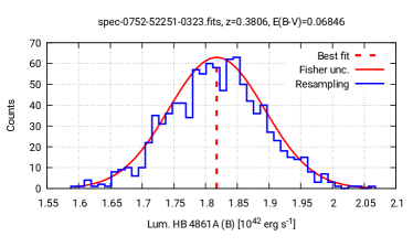
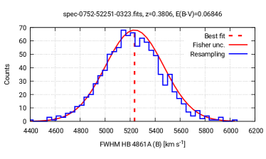
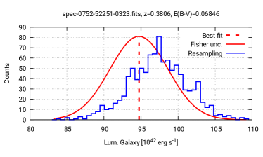
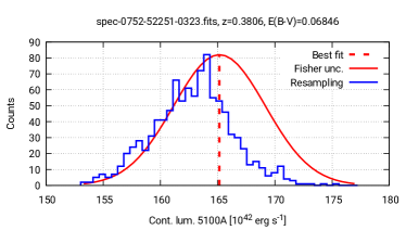
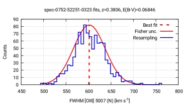
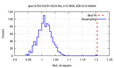
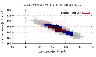
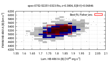
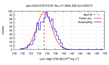
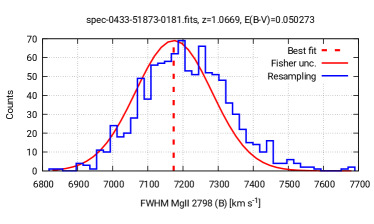
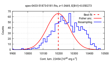
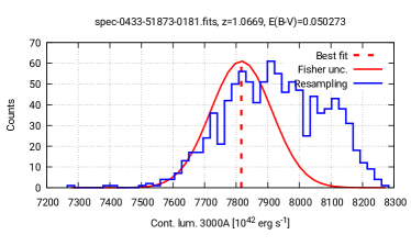
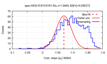
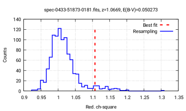
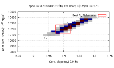
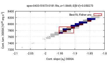
B.5 The QSFit continuum component
The AGN continuum component used in the analysis of the catalog (§3) is a simple power law. However, the QSFit continuum component can be customized to behave as a smoothly broken power law model, to suit those cases where the spectral coverage is sufficiently large to constrain the extra continuum parameters.
The smoothly broken power law is modeled as follows:
| (3) |
where is the break wavelength, is the luminosity density at , is the spectral slope at , is the slope change at , is either or , depending on the sign of , and is the curvature parameter. When or Eq.3 reduces to:
| (4) |
The change of slopes occurs between the wavelengths () and () such that:
| (5) |
hence controls the “sharpness” of the change in slope. In the current QSFit implementation the parameter is constrained to be positive; is constrained in the range , ; is constrained in the range [, 1]; is constrained in the range [, 0.2], although the appropriate limits depends on the available spectral coverage.
B.6 QSFit design, internals and the GFIT framework
In this section we will provide a brief description of the principles
followed while developing QSFit, its most relevant routines, and
the GFIT framework (used for model evaluation). Also, we will
provide the very basic information required to understand the code in
the qsfit.pro file. This is not intended to be a complete
documentation of the code, but rather a quick and very short
introduction to QSFit internals.
Unlike the field of X–ray spectral analysis, there is not yet a well
established and widely accepted procedure to automatically analyze the
Type 1 AGN optical spectra. This is due to the many possible ways the
problem can be approached, and to the different purposes pursued by
the researchers in the field. QSFit is just a first attempt to
fill this gap but, given the above premises, it is likely that the way
it operates will not be suitable to fit particular needs, and likely
the code will require some customization. This implies that the best
way to design QSFit is by providing a neat and short source code
with extensive documentation, easy to read and customize. We went a
little further and carefully separated the procedures which are rather
well established and will unlikely be modified by the user, from those
that are actually related to the specific task of AGN spectral
fitting. The former procedures were collected in a library in the
IDL/Glib and IDL/qsfit/components directories of the
QSFit package, while the latter are all contained in a single file
named qsfit.pro (located in the IDL/qsfit directory).
In the vast majority of cases this is the only file one needs to
modify to customize the fitting process. As a consequence, it is
actually pointless to develop a well defined and user–friendly
interface to customize the fitting process (as is the case for,
e.g. XSPEC, Sherpa, etc.), since the underlying code can
be modified in an unpredictable way. The drawback of this approach is
that the users should become acquainted with the QSFit source code.
On the other hand it provides the greatest flexibility to the user
since it allows to modify every detail of the analysis and implement
very complex recipes. However, in order to facilitate the most common
customization tasks even for unexperienced users, we created a IDL
global variable named !QSFIT_OPT containing the settings a user
may wish to change. The default values for such settings, and their
meaning, can be found in the qsfit_prepare_options routine in
the qsfit.pro file. Moreover, we marked the places in the
source file qsfit.pro where an easy customization can be made,
the with the comment CUSTOMIZABLE. These lines can be easily
modified even without a complete understanding of the remaining code.
The QSFit code relies on the GFIT framework to handle the model
evaluation, parameter definitions and constraints, and the generations
of plots to compare the data and the model. The QSFit framework
relies on the MPFIT minimization routine (Markwardt, 2009),
and its use allowed us to write a very neat code and to always obtain
the best performances in model evaluation, regardless of the
complexity of the model. The documentation for the GFIT framework
can be found in the IDL/Glib/gfit directory. Here we will
shortly describe its usage:
-
•
the GFIT software maintains its whole state in a single structure named
gfit. The information related to the input data, the components to build the model, the parameters in each component, the parameters constraints, the plotting settings, etc. are all stored in this variable. Thegfitstructure is available in an IDL common block with the same name, hence each program unit willing to use it should state the following line at its beginning:COMMON GFIT
-
•
the
gfitstructure is modified by the calls to one of thegfit_*routines, e.g.gfit_add_datato add a data set,gfit_add_compto add a component to the model, etc. -
•
the values in the
gfitstructure can be directly modified by the user, e.g. the mathematical expression for the model will be set intogfit.expr.(0).model, the limits for the host galaxy normalization parameter will be set intogfit.comp.galaxy.norm.limits, etc. An absorption line can easily be included in the model by setting the normalization limits to negative values, e.g.:gfit.comp.LINE_NAME.norm.limits = [-1, 0]; -
•
each time the model is modified (either by adding a component, by freezing or thawing a parameter) the
gfit_compileprocedure should be called. This procedure automatically generates and compile the IDL code needed to evaluate the model, ensuring the best possible performance even with very complex model definitions; -
•
the
gfit_reportand thegfit_plotprocedures are respectively used to generate a report of the GFIT state, and to generate the comparison plot between the model and the data; -
•
the
gfit_runprocedure is used to perform the model minimization through a call tompfit. Once finished, the parameter values and uncertainties are updated. The latter are available in thegfit.compsubstructure, e.g.gfit.comp.continuum.norm.val,gfit.comp.continuum.norm.err, etc.
As discussed above, all the relevant code for QSFit customization
is located in the qsfit.pro file. In the following we will
briefly mention the most relevant routines:
-
•
qsfit_log: this procedure print log messages. All messages are also stored in an internal buffer to be dumped at the end of the analysis; -
•
qsfit_compile: this procedure (re–)compiles the GFIT model. It should be called each time the model is modified; -
•
qsfit_lineset: this function returns the list of “known” emission lines to be considered in the analysis. It can be customized to add/remove emission line components to the model. Disabling a few lines, e.g. the less luminous ones, is the simplest way to significantly speed up the QSFit analysis; -
•
qsfit_prepare: this procedure reads a SDSS DR–10 FITS file and loads data into GFIT internal structure (see §2.8.1). If you wish to read data from another source you should modify this procedure; -
•
qsfit_run: this procedure implements the actual QSFit recipe for model fitting (§2.8.2). If you wish to modify the sequence by which each component is added you should modify this procedure; - •
-
•
qsfit: this is the main function to perform the QSFit analysis, and actually the only one supposed to be directly called by the final user; -
•
qsfit_report: this procedure prints the final report of the QSFit analysis; -
•
qsfit_plot: this procedure generates the plots of the results of the analysis (§B.2); -
•
qsfit_version: this function simply returns a string with the current QSFit version, also stored in the nested structure returned by theqsfitfunction (see §B.3). If you modify theqsfit.profile we suggest to modify this function as well, in order to quickly identify which version generated a given result.
Appendix C Quality flags in the QSFIT catalog
The columns in the QSFIT catalog whose name has a
__QUALITY suffix report the “quality flags” for the
associated quantity (see §A). In this
section we report both the total number and the fraction of sources
(over the total number of sources in the catalog: 71,251) which raised
a flag. Also shown are the total number and the fraction of sources
with no flag raised (i.e. whose __QUALITY entry is equal to
zero), also called “Good” sources with respect to a specific
quantity.
The statistics for the continuum quantities are summarized in Tab. 2, where each of the 5 wavelengths (equally spaced in the logarithmic wavelength range) are shown in the upper part of the table, in the columns labeled W1…W5. The lower part of the table reports the statistics for the 1450Å, 2245Å, 3000Å, 4210Å and 5100Å fixed wavelengths. The statistics for the host galaxy quantities are summarized in Tab. 3. The statistics for the four UV iron components and for the two optical iron quantities are shown in Tab. 4 (upper and lower table respectively). Finally, the statistics for the emission line quantities are shown in Tab. 5 and Tab. 6.
| Quality | W1 | W2 | W3 | W4 | W5 | |||||
|---|---|---|---|---|---|---|---|---|---|---|
| Gooda | 70590 | 99.07% | 70590 | 99.07% | 70588 | 99.07% | 70587 | 99.07% | 70586 | 99.07% |
| Bit 0b | 0 | 0.00% | 0 | 0.00% | 0 | 0.00% | 0 | 0.00% | 0 | 0.00% |
| Bit 1c | 32 | 0.04% | 32 | 0.04% | 32 | 0.04% | 32 | 0.04% | 32 | 0.04% |
| Bit 2d | 4 | 0.01% | 4 | 0.01% | 4 | 0.01% | 4 | 0.01% | 5 | 0.01% |
| Bit 3e | 277 | 0.39% | 277 | 0.39% | 277 | 0.39% | 277 | 0.39% | 277 | 0.39% |
| Bit 4f | 38 | 0.05% | 38 | 0.05% | 40 | 0.06% | 41 | 0.06% | 41 | 0.06% |
| Bit 5g | 320 | 0.45% | 320 | 0.45% | 320 | 0.45% | 320 | 0.45% | 320 | 0.45% |
| Bit 6h | 0 | 0.00% | 0 | 0.00% | 0 | 0.00% | 0 | 0.00% | 0 | 0.00% |
| Quality | 1450Å | 2245Å | 3000Å | 4210Å | 5100Å | |||||
| Gooda | 6587 | 9.24% | 52105 | 73.13% | 60791 | 85.32% | 25325 | 35.54% | 14117 | 19.81% |
| Bit 0b | 64647 | 90.73% | 18962 | 26.61% | 9839 | 13.81% | 45403 | 63.72% | 56806 | 79.73% |
| Bit 1c | 0 | 0.00% | 0 | 0.00% | 6 | 0.01% | 32 | 0.04% | 31 | 0.04% |
| Bit 2d | 0 | 0.00% | 0 | 0.00% | 0 | 0.00% | 4 | 0.01% | 4 | 0.01% |
| Bit 3e | 11 | 0.02% | 123 | 0.17% | 272 | 0.38% | 179 | 0.25% | 102 | 0.14% |
| Bit 4f | 4 | 0.01% | 21 | 0.03% | 34 | 0.05% | 18 | 0.03% | 13 | 0.02% |
| Bit 5g | 2 | 0.00% | 41 | 0.06% | 318 | 0.45% | 297 | 0.42% | 186 | 0.26% |
| Bit 6h | 0 | 0.00% | 0 | 0.00% | 0 | 0.00% | 0 | 0.00% | 0 | 0.00% |
a: All bits set to 0;
b: Bit 0: wavelength is outside the observed range;
c: Bit 1: either the luminosity or its uncertainty are NaN or equal to zero;
d: Bit 2: luminosity relative uncertainty 1.5;
e: Bit 3: either the slope or its uncertainty are NaN or equal to zero;
f: Bit 4: slope hits a limit in the fit;
g: Bit 5: slope uncertainty 0.3;
| Quality | # sources | |
|---|---|---|
| Gooda | 13015 | 18.3% |
| Bit 0b | 53887 | 75.6% |
| Bit 1c | 3727 | 5.2% |
| Bit 2d | 622 | 0.9% |
a: All bits set to 0;
b: Bit 0: fit of galaxy template is not sensible at this redshift;
c: Bit 1: either the luminosity or its uncertainty are NaN or equal to zero;
d: Bit 2: luminosity relative uncertainty 1.5;
| Quality | Iron UV | |||
|---|---|---|---|---|
| Gooda | 46540 | 65.3% | ||
| Bit 0b | 0 | 0.0% | ||
| Bit 1c | 24676 | 34.6% | ||
| Bit 2d | 35 | 0.0% | ||
| Quality | Broad | Narrow | ||
| Gooda | 21449 | 30.1% | 12070 | 16.9% |
| Bit 0b | 48416 | 68.0% | 48416 | 68.0% |
| Bit 1c | 871 | 1.2% | 7466 | 10.5% |
| Bit 2d | 515 | 0.7% | 3299 | 4.6% |
a: All bits set to 0;
b: Bit 0: fit of iron template is not sensible at this redshift;
c: Bit 1: either the luminosity or its uncertainty are NaN or equal to zero;
d: Bit 2: luminosity relative uncertainty 1.5;
| Line | SiIV (B) | CIV (B) | CIII (B) | MgII (B) | NeVI (N) | |||||
|---|---|---|---|---|---|---|---|---|---|---|
| Wavelen. [Å] | 1400 | 1549 | 1909 | 2798 | 3426 | |||||
| Ncomp=1 | 7375 | (97.1%) | 12001 | (58.7%) | 40138 | (93.1%) | 48826 | (74.1%) | 49970 | (100.0%) |
| Ncomp=2 | 220 | (2.9%) | 7709 | (37.7%) | 2916 | (6.8%) | 16397 | (24.9%) | ||
| Ncomp=3 | 1 | (0.0%) | 685 | (3.4%) | 49 | (0.1%) | 661 | (1.0%) | ||
| Ncomp=4 | 39 | (0.2%) | 1 | (0.0%) | 14 | (0.0%) | ||||
| Ncomp=5 | 2 | (0.0%) | ||||||||
| Ncomp=6 | 1 | (0.0%) | ||||||||
| Ncomp=7 | 2 | (0.0%) | ||||||||
| Total | 7596 | 20439 | 43104 | 65898 | 49970 | |||||
| Quality | ||||||||||
| Gooda | 5151 | (67.8%) | 15193 | (74.3%) | 25208 | (58.5%) | 52399 | (79.5%) | 11134 | (22.3%) |
| Bit 0b | 99 | (1.3%) | 67 | (0.3%) | 94 | (0.2%) | 49 | (0.1%) | 4073 | (8.2%) |
| Bit 1c | 62 | (0.8%) | 53 | (0.3%) | 87 | (0.2%) | 86 | (0.1%) | 4373 | (8.8%) |
| Bit 2d | 565 | (7.4%) | 930 | (4.6%) | 6493 | (15.1%) | 654 | (1.0%) | 22811 | (45.6%) |
| Bit 3e | 661 | (8.7%) | 861 | (4.2%) | 4357 | (10.1%) | 2005 | (3.0%) | 13585 | (27.2%) |
| Bit 4f | 37 | (0.5%) | 33 | (0.2%) | 45 | (0.1%) | 77 | (0.1%) | 1718 | (3.4%) |
| Bit 5g | 699 | (9.2%) | 1922 | (9.4%) | 9337 | (21.7%) | 8495 | (12.9%) | 15206 | (30.4%) |
| Bit 6h | 108 | (1.4%) | 74 | (0.4%) | 913 | (2.1%) | 1329 | (2.0%) | 2161 | (4.3%) |
| Bit 7i | 1642 | (21.6%) | 2609 | (12.8%) | 4239 | (9.8%) | 3426 | (5.2%) | 5105 | (10.2%) |
| Line | OII (N) | NeIII (N) | Hd (B) | Hg (B) | Hb (N) | |||||
| Wavelen. [Å] | 3727 | 3869 | 4103 | 4342 | 4863 | |||||
| Ncomp=1 | 40712 | (100.0%) | 36424 | (100.0%) | 29215 | (95.2%) | 23450 | (91.5%) | 17780 | (100.0%) |
| Ncomp=2 | 1465 | (4.8%) | 2159 | (8.4%) | ||||||
| Ncomp=3 | 4 | (0.0%) | 18 | (0.1%) | ||||||
| Ncomp=4 | ||||||||||
| Ncomp=5 | ||||||||||
| Ncomp=6 | ||||||||||
| Ncomp=7 | ||||||||||
| Total | 40712 | 36424 | 30684 | 25627 | 17780 | |||||
| Quality | ||||||||||
| Gooda | 21029 | (51.7%) | 11498 | (31.6%) | 8790 | (28.6%) | 20393 | (79.6%) | 5123 | (28.8%) |
| Bit 0b | 2156 | (5.3%) | 1028 | (2.8%) | 3375 | (11.0%) | 32 | (0.1%) | 376 | (2.1%) |
| Bit 1c | 2184 | (5.4%) | 1525 | (4.2%) | 2049 | (6.7%) | 89 | (0.3%) | 451 | (2.5%) |
| Bit 2d | 9292 | (22.8%) | 13495 | (37.0%) | 8711 | (28.4%) | 2011 | (7.8%) | 8355 | (47.0%) |
| Bit 3e | 9393 | (23.1%) | 10442 | (28.7%) | 7994 | (26.1%) | 374 | (1.5%) | 4197 | (23.6%) |
| Bit 4f | 819 | (2.0%) | 574 | (1.6%) | 892 | (2.9%) | 42 | (0.2%) | 162 | (0.9%) |
| Bit 5g | 6039 | (14.8%) | 5044 | (13.8%) | 9380 | (30.6%) | 1298 | (5.1%) | 546 | (3.1%) |
| Bit 6h | 953 | (2.3%) | 1064 | (2.9%) | 1967 | (6.4%) | 167 | (0.7%) | 104 | (0.6%) |
| Bit 7i | 3176 | (7.8%) | 2670 | (7.3%) | 11407 | (37.2%) | 3307 | (12.9%) | 199 | (1.1%) |
a: All bits set to 0;
b: Bit 0: either the luminosity or its uncertainty are NaN or equal to zero;
c: Bit 1: luminosity relative uncertainty 1.5;
d: Bit 2: either the FWHM or its uncertainty are NaN or equal to zero;
e: Bit 3: FWHM value hits a limit in the fit;
f: Bit 4: FWHM relative uncertainty 2;
g: Bit 5: either the Voff or its uncertainty are NaN or equal to zero;
h: Bit 6: Voff value hits a limit in the fit;
i: Bit 7: Voff uncertainty 500 km s-1;
| Line | Hb (B) | OIII (N) | OIII (N) | HeI (B) | NII (N) | |||||
|---|---|---|---|---|---|---|---|---|---|---|
| Wavelen. [Å] | 4863 | 4959 | 5007 | 5876 | 6549 | |||||
| Ncomp=1 | 15405 | (86.7%) | 16372 | (100.0%) | 16233 | (100.0%) | 7209 | (96.2%) | 2841 | (100.0%) |
| Ncomp=2 | 2323 | (13.1%) | 280 | (3.7%) | ||||||
| Ncomp=3 | 50 | (0.3%) | 2 | (0.0%) | ||||||
| Ncomp=4 | ||||||||||
| Ncomp=5 | ||||||||||
| Ncomp=6 | ||||||||||
| Ncomp=7 | ||||||||||
| Total | 17778 | 16372 | 16233 | 7491 | 2841 | |||||
| Quality | ||||||||||
| Gooda | 14714 | (82.8%) | 0 | (0.0%) | 14377 | (88.6%) | 1351 | (18.0%) | 1602 | (56.4%) |
| Bit 0b | 37 | (0.2%) | 351 | (2.1%) | 33 | (0.2%) | 1164 | (15.5%) | 50 | (1.8%) |
| Bit 1c | 42 | (0.2%) | 322 | (2.0%) | 30 | (0.2%) | 407 | (5.4%) | 64 | (2.3%) |
| Bit 2d | 1194 | (6.7%) | 3384 | (20.7%) | 500 | (3.1%) | 3127 | (41.7%) | 690 | (24.3%) |
| Bit 3e | 280 | (1.6%) | 1838 | (11.2%) | 1321 | (8.1%) | 1631 | (21.8%) | 476 | (16.8%) |
| Bit 4f | 16 | (0.1%) | 111 | (0.7%) | 11 | (0.1%) | 236 | (3.2%) | 6 | (0.2%) |
| Bit 5g | 1072 | (6.0%) | 16372 | (100.0%) | 87 | (0.5%) | 2838 | (37.9%) | 84 | (3.0%) |
| Bit 6h | 76 | (0.4%) | 0 | (0.0%) | 32 | (0.2%) | 858 | (11.5%) | 20 | (0.7%) |
| Bit 7i | 1533 | (8.6%) | 0 | (0.0%) | 17 | (0.1%) | 2956 | (39.5%) | 64 | (2.3%) |
| Line | Ha (N) | Ha (B) | NII (N) | SII (N) | SII (N) | |||||
| Wavelen. [Å] | 6565 | 6565 | 6583 | 6716 | 6731 | |||||
| Ncomp=1 | 2924 | (100.0%) | 2780 | (95.1%) | 2843 | (100.0%) | 2483 | (100.0%) | 2417 | (100.0%) |
| Ncomp=2 | 140 | (4.8%) | ||||||||
| Ncomp=3 | 3 | (0.1%) | ||||||||
| Ncomp=4 | ||||||||||
| Ncomp=5 | ||||||||||
| Ncomp=6 | ||||||||||
| Ncomp=7 | ||||||||||
| Total | 2924 | 2923 | 2843 | 2483 | 2417 | |||||
| Quality | ||||||||||
| Gooda | 1818 | (62.2%) | 2818 | (96.4%) | 2014 | (70.8%) | 1136 | (45.8%) | 1090 | (45.1%) |
| Bit 0b | 14 | (0.5%) | 7 | (0.2%) | 12 | (0.4%) | 42 | (1.7%) | 91 | (3.8%) |
| Bit 1c | 42 | (1.4%) | 5 | (0.2%) | 38 | (1.3%) | 64 | (2.6%) | 80 | (3.3%) |
| Bit 2d | 196 | (6.7%) | 39 | (1.3%) | 161 | (5.7%) | 703 | (28.3%) | 470 | (19.4%) |
| Bit 3e | 889 | (30.4%) | 9 | (0.3%) | 629 | (22.1%) | 608 | (24.5%) | 829 | (34.3%) |
| Bit 4f | 13 | (0.4%) | 1 | (0.0%) | 5 | (0.2%) | 23 | (0.9%) | 32 | (1.3%) |
| Bit 5g | 17 | (0.6%) | 30 | (1.0%) | 19 | (0.7%) | 356 | (14.3%) | 205 | (8.5%) |
| Bit 6h | 2 | (0.1%) | 1 | (0.0%) | 21 | (0.7%) | 19 | (0.8%) | 14 | (0.6%) |
| Bit 7i | 14 | (0.5%) | 44 | (1.5%) | 24 | (0.8%) | 55 | (2.2%) | 51 | (2.1%) |
a: All bits set to 0;
b: Bit 0: either the luminosity or its uncertainty are NaN or equal to zero;
c: Bit 1: luminosity relative uncertainty 1.5;
d: Bit 2: either the FWHM or its uncertainty are NaN or equal to zero;
e: Bit 3: FWHM value hits a limit in the fit;
f: Bit 4: FWHM relative uncertainty 2;
g: Bit 5: either the Voff or its uncertainty are NaN or equal to zero;
h: Bit 6: Voff value hits a limit in the fit;
i: Bit 7: Voff uncertainty 500 km s-1;