Splashback shells of Cold Dark Matter halos

Abstract

The density field in the outskirts of dark matter halos is discontinuous due to a caustic formed by matter at its first apocenter after infall. In this paper, we present an algorithm to identify the “splashback shell” formed by these apocenters in individual simulated halos using only a single snapshot of the density field. We implement this algorithm in the code Shellfish (SHELL Finding In Spheroidal Halos) and demonstrate that the code identifies splashback shells correctly and measures their properties with an accuracy of $<5\%$ for halos with more than 50,000 particles and mass accretion rates of $\Gamma_{\textrm{DK14}}>0.5$. Using Shellfish, we present the first estimates for several basic properties of individual splashback shells, such as radius, $R_{\textrm{sp}}$, mass, and overdensity, and provide fits to the distribution of these quantities as functions of $\Gamma_{\textrm{DK14}}$, $\nu_{\textrm{200m}}$, and $z.$ We confirm previous findings that $R_{\textrm{sp}}$ decreases with increasing $\Gamma_{\textrm{DK14}}$, but we show that independent of accretion rate, it also decreases with increasing $\nu_{\textrm{200m}}$. We also study the 3D structures of these shells and find that they generally have non-ellipsoidal oval shapes. We find that splashback radii estimated by Shellfish are $20\%-30\%$ larger than those estimated in previous studies from stacked density profiles at high accretion rates. We demonstrate that the latter are biased low due to the contribution of high-mass subhalos to these profiles and show that using the median instead of mean density in each radial bin mitigates the effect of substructure on density profiles and removes the bias.

1. Introduction

In the Cold Dark Matter (CDM) paradigm of structure formation, dark matter halos form via the collapse of density peaks in the initial random Gaussian perturbation field. In the commonly used “tophat model” the peak density contrast profile is approximated as uniform within a given radius (e.g., Tolman, 1934). The constant overdensity in such approximations results in a uniform collapse time for different radial shells and a single well-defined collapse time for the peak. This, along with the assumption that virial equilibrium is reached immediately following collapse, allows one to predict the density contrast within the boundary of the collapsed objects (Gunn & Gott, 1972; Heath, 1977; Lahav et al., 1991).

Accordingly, the most commonly used boundary definition for CDM halos is the radius, $R_{\Delta},$ enclosing a given density contrast $\Delta\equiv\rho(<r)/\rho_{\rm ref}$, where $\rho_{\rm ref}$ is a reference density, taken to be either the mean density of the universe, $\rho_{\rm m}$, or the critical density for closure, $\rho_{\rm crit}$, at the redshift of observation. The corresponding enclosed mass is given by

$$M(<R_{\Delta})=\Delta\rho_{\rm ref}\ \frac{4}{3}\pi R_{\Delta}^{3}.$$ (1)

The value of $\Delta$ is usually motivated by tophat collapse models.

However, the overdensity profile in real Gaussian peaks is not constant, but decreases with increasing radius (see, e.g., Figure 2 in Dalal et al., 2010). Because the overdensity within a given radius controls the timing of the collapse, the collapse of different radial shells in such peaks is extended in time. Real halos also undergo mergers during their formation, which further redistribute mass within them. Real CDM halos thus do not have an edge at the density contrast predicted by simple uniform peak collapse models (see, e.g., Kravtsov & Borgani, 2012; More et al., 2015), meaning that $R_{\Delta}$ radii are a rather arbitrary definition of halo extent and do not correspond to any particular feature in the density profile or in the profiles of other physical properties (e.g., Diemer et al., 2013a). This arbitrariness may be problematic when this radius is used to classify objects into groups which are meant to be qualitatively distinct from one another, such as subhalos and isolated halos. Indeed, multiple recent studies have suggested that a significant fraction of the halo assembly bias effect may be due to the fact that some subhalos which have orbited larger hosts are misclassified as isolated halos when $R_{\Delta}$ is used as a halo boundary for classification (Wang et al., 2009; Wetzel et al., 2014; Sunayama et al., 2016; Zentner et al., 2016). However, these so-called “backsplash” halos would still necessarily be contained within their hosts’ splashback shells, meaning that switching to a splashback-based definition could help alleviate this issue.

Furthermore, regardless of the choice of $\Delta$ or $\rho_{\rm ref}$, contrast-based radius and mass definitions encounter several problems when the mass accretion histories of halos are estimated. First, as mentioned above, during major mergers there is mass redistribution within halos, with a non-trivial amount of mass moving to radii outside of $R_{\Delta}$ for typical values of $\Delta$ (Kazantzidis, Zentner, & Kravtsov, 2006). This causes spherical overdensity masses to be non-additive during mergers in excess to the degree that would be expected purely from slingshot processes. Second, the evolution of both $\rho_{\rm m}$ and $\rho_{\rm crit}$ with time causes evolution in $R_{\Delta}$ and $M_{\Delta}$, even for completely static density profiles. This “pseudo-evolution” of halo radius and mass typically results in the near doubling of mass of Milky Way-sized halos between $z=1$ and $z=0$, even when there is no accretion of new mass (Diemer et al., 2013b).

Given the problems with the standard $R_{\Delta}$ definition, one can ask whether there is a more physical way to define halo boundary, one which would separate the matter that has already collapsed (i.e., orbited within halo at least once) and matter that is still infalling onto halo for the first time. In collapse models of spherical and ellipsoidal peaks with power law density profiles, such a boundary exists and is associated with a sudden drop in the density profile of collapsed halos (Fillmore & Goldreich, 1984; Bertschinger, 1985; Adhikari et al., 2014; Shi, 2016). The drop is due to the caustic formed by the “pile up” of mass elements that have just reached the apocenter of their first orbits and is thus the maximum radius of matter that has orbited through halo at least once.

Recently, such drops in the density profile have also been detected in both simulated and real CDM halos (Diemer & Kravtsov, 2014; Adhikari et al., 2014; More et al., 2015, 2016; Adhikari et al., 2016). The most distant apocenters of orbits in real halos form a surface that we will call the splashback shell. This shell can be viewed as the halo boundary. Due to the assumption of spherical symmetry, all previous studies have necessarily been restricted to analyzing the characteristic scale of this shell, the splashback radius, $R_{\rm sp}$.

The primary challenge in using the splashback shell as a physical boundary definition for halos is that it is technically challenging to detect and quantify in individual objects, both in cosmological simulations and in observations. The key problem is that splashback shells are generally located at low densities, where the presence of individual neighboring halos or filaments can complicate the interpretation of the density field.

Consequently, analyses of the splashback radius have so far been carried out using stacked radial density profiles of either mass or subhalo abundance (Diemer & Kravtsov, 2014; Adhikari et al., 2014, 2016; More et al., 2015, 2016). After stacking, $R_{\rm sp}$ for the population is operationally defined as the radius of the steepest logarithmic slope, ${\rm d}\ln{\rho}/{\rm d}\ln{r}$ (or ${\rm d}\ln{n_{\rm sub}}/{\rm d}\ln{r}$). In principle, this procedure averages out the noise in the individual profiles, allowing for comparisons of the splashback radius between different halo populations. However, stacking of different halo profiles can also “wash out” the sharp density gradient associated with the splashback shells, if such shells exhibit scatter for individual halos.

Studies of the splashback radius based on stacked density profiles have shown that there is a strong relation between $R_{\rm sp}/R_{\rm 200m}$ and halo mass accretion rate, $\Gamma_{\rm DK14}$, (Diemer & Kravtsov, 2014; More et al., 2015). Where $\Gamma_{\rm DK14}$ is defined as

$$\Gamma_{\rm DK14}\equiv\frac{\ln{M_{\rm 200m}(z_{i+1})}-\ln{M_{\rm 200m}(z_{i})}}{\ln{a(z_{i+1})}-\ln{a(z_{i})}},$$ (2)

here $z_{i}$ come from a set of redshift intervals which are separated by roughly a dynamical time. Previous studies have used the intervals $z_{i}=\{0,0.5,1,2,4\},$ a convention which we shall continue to use in this paper (although future studies may benefit strongly from revisiting this choice in definition). Such a dependence is expected theoretically due to the contraction of particle orbits in a rapidly deepening potential of high-$\Gamma_{\rm DK14}$ halos (Diemer & Kravtsov, 2014; Adhikari et al., 2014).

Hints of density steepening due to the splashback radius in the mass and galaxy distribution around individual clusters have been reported in several recent studies (Rines et al., 2013; Tully, 2015; Patej & Loeb, 2016; Umetsu & Diemer, 2017). Interestingly, the first reliable observational estimates of the splashback radius from the radial number density profiles of satellite galaxies in clusters are in tension with the predictions of simulations (More et al., 2016).

The operational simplicity of the stacked-profile approach makes it very useful, particularly when comparing simulations to observations, but it is not without weaknesses. First, spherical averaging discards all information about the shapes of the splashback shells, even though the filamentary nature of the cosmic web causes accretion to be highly aspherical, which implies that splashback shells should also be highly aspherical. Second, the stacking procedure removes information about individual halos, making it impossible to study the evolution of a single halo’s shell over time, the properties of subhalos contained within shells, or the scatter around mean relations. Third, the relationship between the splashback radius estimated from the stacked profiles and the underlying distribution of individual splashback radii is unknown and can be complicated. In particular, as we show in section 4.3, the contribution of massive subhalos in a minority of individual density profiles introduces significant bias in the estimate of the splashback radius derived from stacked profiles.

To address these issues and to explore the properties of splashback shells around individual halos, in this paper we present an algorithm which identifies the splashback shells around individual halos using single particle snapshots from cosmological $N$-body simulations, and an implementation of the algorithm in the code Shellfish (SHELL Finding In Spheroidal Halos), which we use to generate halo catalogs with measured splashback shells and perform analyses of their basic properties, such as radius and shape, and quantify their relationships to other halo properties, such as mass accretion rate and peak height. A public version of Shellfish, along with tutorials and documentation can be found at github.com/phil-mansfield/shellfish with a Digital Object Identifier (DOI) given by SHELLFISH_2017.

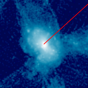
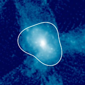
This paper is organized as follows. An overview of our method is shown in Figure 1 and our key result, the $\Gamma_{\rm DK14}$ - $R_{\rm sp}$ relation for individual halos, is shown in Figure 9. In section 2 we describe our algorithm to identify the splashback shells from a halo’s particle distribution, in section 3 we present extensive tests of the correctness and convergence properties of the shells identified by our implementation of the algorithm. In section 4 we discuss the shapes of the splashback shells and present the relation between shell size and mass accretion rate. We compare the latter relation to that derived from the stacked profiles, and show that the stacking introduces significant bias in the estimates of the splashback radius of rapidly growing halos. We summarize our results in section 5. Appendix A contains a description of a high performance ray-tracing algorithm that we developed as a component of Shellfish.

A reader not interested in the details of the algorithm itself, but only in the properties of identified shells can skip directly to section 4. We caution, however, that proper interpretation of the issues discussed in section 4 requires at least a basic understanding of our shell finding algorithm.

2. Methods

2.1. Simulations

The analysis in this paper uses a subset of the suite of simulations first introduced in Diemer & Kravtsov (2014). These simulations have box sizes between $62.5h^{-1}\,\rm Mpc$ and $500h^{-1}\,\rm Mpc$, allowing us to study halos with a wide range of masses and accretion rates and use the same cosmological parameters as the Bolshoi simulation suite (Klypin et al., 2011): $\Omega_{\rm m}=1-\Omega_{\Lambda}=0.3$, $\Omega_{\rm b}=0.0469$, $H_{0}$ = 70 km s^-1 Mpc^-1, $\sigma_{8}=0.82$, and $n_{\rm s}=0.95$ (Komatsu et al., 2011). All simulations followed the evolution of $1024^{3}$ particles using the Gadget-2 code (Springel, 2005), starting at $z=49$, and were run with the timestep parameter of $\eta=0.025.$ Simulation-specific parameters can be found in Table 1. Halo catalogs were generated using the Rockstar halo finder (Behroozi et al., 2013) and main progenitor lines were found through the merger tree code consistent-trees (Behroozi et al., 2013).

Table 1Simulation parameters

Name	$L$	$m_{\rm p}$	$\epsilon$	$M_{\rm 200m,min}$	$M_{\rm 200m,max}$
Units	$h^{-1}$ Mpc	$h^{-1}\,M_{\odot}$	$h^{-1}$ kpc	$h^{-1}\,M_{\odot}$	$h^{-1}\,M_{\odot}$
L0500	500	$8.7\times 10^{9}$	14.0	$4\times 10^{14}$	-
L0250	250	$1.1\times 10^{9}$	5.8	$5\times 10^{13}$	$2\times 10^{14}$
L0125	125	$1.4\times 10^{8}$	2.4	$7\times 10^{12}$	$5\times 10^{13}$
L0063	62.5	$1.7\times 10^{7}$	1.0	$9\times 10^{11}$	$7\times 10^{12}$

2.2. Algorithm Description

Figure 1.— An overview of the steps in our shell-finding algorithm for a cluster-sized halo (This halo is also shown in Figure 2 below). Figure 1 shows a random line of sight traced through this halo’s density field (see §2.2.1 and Appendix A). Figures 1 shows a density profile measured along along this line of sight before smoothing (black line) and after smoothing with a Savitzky-Golay filter (red line). The arrow indicates the point of steepest slope in the smoothed profile (see §2.2.2). Figure 1 shows the points of steepest slope for the 256 lines of sight in the viewing plane and shows the point classification that the algorithm generates for these points (see Appendix B). The white curve shows the filtering spline created during the point selection process. Points which are close enough to this curve to pass the filter are shown in white and those which are too far away are shown in red. Figure 1 shows the cross-section of the best fit Penna-Dines surface from the overall distribution of splashback points from 100 randomly oriented planes in which such a procedure was carried out (see §2.2.4). See the text in the corresponding sections for details. All analysis is done with the parameter values listed in Table 2, but the underlying images are rendered using spherical kernels of radius $0.05R_{\rm 200m}$ to make the structures around halos more clear.

Our aim is to develop an algorithm which can identify splashback shells around halos using only their density distribution at a single point in time. In other words, this will be an algorithm which uses no dynamical information about the halo’s particles and will rely solely on identifying the density caustic generated by the splashback shell. This restriction would allow such an algorithm to work on simulations that are only sparsely sampled in time.

Relaxing this restriction allows for alternative measurements of $R_{\rm sp}$ which can leverage the full dynamical information of the simulation. For example, Diemer (2017) develops an algorithm, Sparta, for finding splashback radii by locating the apocenters of orbiting particles which requires access to approximately 100 snapshots over the lifetime of the target halos. An extended comparison between Sparta and Shellfish can be found in Diemer et al. (2017).

Below we describe such an algorithm which does not require any dynamical information and demonstrate that it identifies correct splashback shells, provided that target halos are resolved with a sufficient number of particles (see section 3) and provided that target halos are not embedded in very dense environments (see section 4.3).

Specifically, our algorithm consists of four steps:

1. The density field is sampled along tens of thousands 1-d lines of sight anchored at the center of a halo. The specific design decisions governing how the lines of sight are oriented and how densities along them are estimated are described in section 2.2.1 and Appendix A, respectively, and are depicted in Figure 1.

2. The locations of the steepest slope in the density profiles of each line of sight are estimated using a smoothing filter. This part of the algorithm is described in section 2.2.2 and is depicted in Figure 1.

3. The set of profiles is pruned to remove the profiles where the point of steepest slope corresponds to the splashback associated with a nearby halo or filament. The pruning procedure is described in section 2.2.3 and Appendix B and is depicted in Figure 1.

4. We fit the 3-d shape of the shell with a smooth, flexible, functional form using the locations of the steepest slope in the profiles that remain after the pruning step. This is described in section 2.2.4 and is depicted in Figure 1.

The design choices made in step 1 are the most important for ensuring good performance of the algorithm and the design choices made in step 3 are the most important for ensuring that the identified shells are correct.

The free parameters of the algorithm that will be introduced and discussed in the subsequent sections are summarized in Table 2. The logic and procedures of specific parameter choices are discussed in Appendix .

2.2.1 Density estimation along lines of sight

To construct a density profile along a given line of sight we must choose a way to interpolate particle positions and masses onto that line. For simplicity, we choose to approximate particles as tophat spheres of radius $R_{\rm kernel}$ uniform density. Other choices, such as tetrahedral, trilinear, or tricubic tessellations of phase space (e.g., Abel et al., 2012; Hahn & Angulo, 2016), are also implemented in Shellfish and could in principle be used in this work. However, we find that these estimators converge slowly and do not allow splashback shells for halos with $N_{\rm 200m}\lesssim 10^{7}$ to be identified reliably and thus do not use them in practice. A detailed convergence study of phase space density estimators will be the subject of future work.

The algorithm represents every line of sight as an array of $N_{\rm bins}$ bins logarithmically distributed between the radii $R_{\rm min}$ and $R_{\rm max}$. The density along a line of sight, $l$, which passes through a set of constant-density spheres is given by

$$\rho_{l}(r)=\sum_{i=0}^{i<N}\mathbb{I}_{{\rm intr},il}\rho_{i}H(r-r_{\rm in})H(r_{\rm out}-r).$$ (3)

Here, $i$ indexes over all particles, $\mathbb{I}_{{\rm intr},il}$ is an indicator function which is $1$ if $l$ intersects with the sphere of particle $i$ and is $0$ otherwise, $\rho_{i}$ is the density of sphere $i$, $H$ is the Heaviside step function, and $r_{\rm in}$ and $r_{\rm out}$ are the distances to entrance and exit intersection points of $l$ for a given sphere, respectively.

Evaluating Equation 3 is easy if a conventional estimator (such as cloud-in-cell or SPH) is used to write densities to an intermediate grid before they are translated onto the lines of sight, since the grid cell that corresponds to a point at radius $r$ of given ray can be calculated in $O(1)$ operations. However, using an intermediate grid has a number of disadvantages. First, maintaining the high-resolution grid required to accurately measure the contours of the splashback shell consumes a large amount of memory. This restricts the number of halos which can be maintained in memory at once; when generating large catalogs of shells, this can force particle catalogs to be read many times, leading to a significant performance cost. Second, writing the density estimate to a grid is expensive as it involves either an exact rasterization scheme (see, for example, Powell & Abel 2014) of the objects, or Monte Carlo sampling of each solid with sufficiently many points to eliminate shot noise in each cell. Both approaches also require that density estimates are calculated for grid cells which are not intersected by any line of sight. Third, introducing an intermediate grid reduces the fidelity of the line of sight density estimates due to pixelation. This is most apparent as small radii.

We find that in practice these three disadvantages, particularly the second, are significant and make the use of grids for density estimation undesirable. For this reason we evaluate Equation 3 by directly computing the intersection radii between every line of sight and every sphere with no intermediary grid. Attempting this evaluation naively would be computationally intensive, so we use a specialty ray-tracing algorithm, described in the Appendix A, which takes advantage of the fact that the vast majority of the terms in Equation 3 are zero. This algorithm speeds up density assignment by several orders of magnitude compared to both the brute-force geometric approach and the grid-based approach, while still maintaining a comparatively light memory footprint.

The nature of the ray-tracing algorithm requires that the lines of sight are confined in $N_{\rm planes}$ planes and are uniformly spaced in polar angle within these planes. Each plane then contains $N_{\rm los}$ lines of sight within it. This means that the line shown in in Figure 1 could not be evaluated alone and would need to be evaluated simultaneously along with several hundred other other profiles within the viewing plane. This turns out to be a convenient configuration for later steps in the shell finding algorithm.

2.2.2 Measuring the Point of the steepest slope for line of sight profiles

After the density estimation step, we smooth the density profiles of each line of sight using a fourth order Savitzky-Golay filter (Savitzky & Golay, 1964) with a window length of $N_{\rm SG}$ bins in $\log r$ - $\log\rho$ space. A filter is necessary because a high precision determination of $r_{\rm steep}$ requires that $N_{\rm bin}$ be large, but using a large number of bins allows for noise in low-density regions. For bins in which $\rho(r)=0$, the density is set equal to a small background density value, $\rho_{\rm bg}$. Once the density profile of a line of sight is smoothed, we find the radius of the steepest logarithmic slope, $r_{\rm steep}$.

We choose to use a Savitzky-Golay filter because it is effective at removing small scale noise and because it generally doesn’t move the location of the point of steepest slope, even for large window sizes.

We find that the best results are obtained for $N_{\rm SG}\approx N_{\rm bin}/4$ to $N_{\rm bin}/2$, as this allows the filter to remove even moderately large features, such as subhalos. The exact value chosen is given in Table 2. For most lines of sight, the density drop associated with crossing the splashback shell is the most prominent feature in the profile, and thus such an aggressive filter window does not remove it. The smoothing process will flatten the slope at $r_{\rm steep}$, but the actual value of the slope is not used by our algorithm.

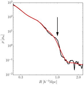
This process is illustrated in Figure 1, which shows the line of sight highlighted in Figure 1. The black curve shows the raw profile after the density estimation step, the red curve shows the profile after applying a Savitzky-Golay filter with a window size of $N_{\rm SG}=N_{\rm bin}/2$. The vertical arrow shows $r_{\rm steep}$ for the smoothed profile. This figure demonstrates several key points. First, the discontinuity due the splashback shell is very strong. Second, the unsmoothed profile contains several points with slopes steeper than the splashback discontinuity due to particle noise. Lastly, the location of $r_{\rm steep}$ has not moved significantly between the smoothed and unsmoothed profiles.

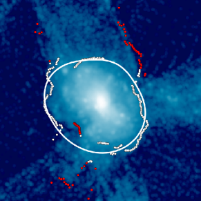
As mentioned in section 2.2.1 (see also Appendix A), the density estimation step of our algorithm requires that lines of sight are confined to a set of planes. The locations of $r_{\rm steep}$ for 256 such lines of sight are shown in Figure 1. This illustrates that, generally, the values of $r_{\rm steep}$ found by this step are in good agreement with the visual appearance of density discontinuities. However, some of the density discontinuities are clearly not associated with the halo itself but are due to nearby filaments or nearby halos. Although this happens in the minority of lines of sight, these can bias the shape of the inferred splashback shell significantly. Therefore, the algorithm makes an additional step in which lines of sight for which the steepest slope points are likely associated with other halos and filaments are pruned from the set.

2.2.3 Filtering out problematic steepest slope points

We remove lines of sight with points of steepest slope that are likely to be associated with other halos and filaments candidate points through an additional filtering step. Filaments have their own elongated splashback shells which are created by the apocenters of matter accreted onto filaments from surrounding void regions. The density jumps associated with these surfaces are comparable to those found around halos. Therefore, it is difficult to differentiate between steepest slope points caused by central halos splashbacks and points caused by filament splashbacks using only the information contained in a single line of sight profile. We experimented with a number of different heuristic approaches of this type and found that they generally require extensive fine-tuning and are, at best, modestly effective at removing filament points.

To classify the splashback points, we consider all of the splashback points within a given plane simultaneously and filter out points which deviate too sharply from the locations of their neighbors. We do this by heuristically constructing a filtering loop, a curve which smoothly passes close to most of the plane’s candidate points but which is too stiff to accommodate sharp changes in radius. We then remove points which are too far away from the filtering loop.

Our filtering algorithm employs a spline curve to approximate the shape of the splashback in a given slice and is described in detail in Appendix B. The algorithm introduces two new free parameters, $\eta$, which controls the strictness of the filter and the “stiffness” of the loop, and $N_{\rm rec}$, which affects the angular resolution of the filtering loop. Larger values of $\eta$ will remove outliers more aggressively, but would also likely prune a larger number of points associated with halo. Qualitatively, points which come from features that deviate by more than $R_{\rm max}/\eta$ from neighboring regions on angular scales of $2\pi/2^{N_{\rm rec}}$ will be removed from the set of lines of sight.

2.2.4 Fitting the shape of the splashback shell

After the filtering step, we fit the remaining points using a family of spheroidal functions introduced by Penna & Dines (2007, hereafter “Penna-Dines functions”). A Penna-Dines function of order $P$ is defined by $2P^{2}$ coefficients, $c_{ijk}$, where $i$ and $j$ range from 0 to $P-1$ and $k$ ranges from 0 to 1. The shape of a shell with a particular set of coefficients is given by the function

$$r(\phi,\theta)=\sum_{i,j=0}^{P-1}\sum_{k=0}^{1}c_{ijk}\sin^{i+j}\theta\ \cos^{k}\theta\ \sin^{j}\phi\ \cos^{i}\phi,$$ (4)

where $\theta$ is the polar angle and $\phi$ is the azimuthal angle. Penna-Dines functions are similar to spherical harmonics in that adding higher order terms allows for the representation of increasingly aspherical shells. We choose to fit these functions because their low order forms are qualitatively similar to the shapes found in splashback shells (this class of functions is specifically designed to represent lobed shapes) and because an optimal fit can be found through the relatively simple and efficient pseudoinverse matrix operation.

Namely, for a set of $N$ points with coordinates given by $r_{n}=\sqrt{x_{n}^{2}+y_{n}^{2}+z_{n}^{2}}$, the best fit coefficients can be computed by the operation

$$c_{ijk}=r_{n}^{2P-1}M^{T}(MM^{T})^{-1}.$$ (5)

Here, $r_{n}^{2P-1}$ is a height $N$ vector containing the radii of every point and $M$ is a $N\ \times\ 2P^{2}$ matrix with elements

$$M_{i+jP+kP^{2},n}=r_{n}^{2P-1-i-j-k}x_{n}^{i}y_{n}^{j}z_{n}^{k}.$$ (6)

2.3. Definitions of basic splashback shell properties

While a full set of Penna-Dines coefficients is necessary for computing subhalo/particle membership and for visualizing shells, it is also useful to encapsulate key properties of the splashback shells in a few representative parameters. To this end, we use a set of properties which parameterize the shape of the splashback shells: $R_{\rm sp}$, the volume-equivalent splashback radius; $\rho_{\rm sp}$, the net density of shell; $a_{\rm sp}$, $b_{\rm sp}$, and $c_{\rm sp}$, the inertia tensor equivalent major axes of the shell; $E_{\rm sp}$, the shell ellipticity; and $A_{\rm sp}$, the shell asphericity:

$$R_{\rm sp} \equiv\left(\frac{3V_{\rm sp}}{4\pi}\right)^{1/3}$$ (7)

$$\rho_{\rm sp} =M_{\rm sp}/V_{\rm sp}$$ (8)

$$\ a_{\rm sp},~{}b_{\rm sp},~{}c_{\rm sp} \equiv{\rm Axes}(I_{x},~{}I_{y},~{}I_{z})$$ (9)

$$E_{\rm sp} \equiv\frac{a_{\rm sp}}{c_{\rm sp}}-1$$ (10)

$$A_{\rm sp} \equiv 1-\frac{S_{\rm sp}}{(36\pi V_{\rm sp}^{2})^{1/3}}$$ (11)

Here, $V_{\rm sp}$ is the volume enclosed by the shell, $M_{\rm sp}$ is the mass of all the particles contained within the shell, $S_{\rm sp}$ is the surface area of the shell, and Axes($I_{x}$, $I_{y}$, $I_{z}$) is a function which computes the axes of a uniform density ellipsoidal shell which has the moments of inertia $I_{x}$, $I_{y}$, and $I_{z}$. The construction of this function is described in Appendix D. In Equation 10, we take the standard convention that $a_{\rm sp}$ is the major axis and $c_{\rm sp}$ is the minor axis.

$E_{\rm sp}$ is defined such that it is zero for a sphere and increases for increasingly elliptical shells. $A_{\rm sp}$ is defined such that it is zero for a sphere and increases for increasingly aspherical shells. Our numerical experiments with randomly-shaped shells indicate that it is probable that prolate ellipsoids are the surfaces which minimize $A_{\rm sp}$ for a given value of $E_{\rm sp}$.

Figure 2.— Density slices of six halos are shown within boxes of size $5R_{\rm 200m}$ along with cross-sections of each halo’s splashback shell identified by our algorithm (white lines) and cross-sections of spheres with the same volume as the splashback shell (black circles). The six halos were picked randomly by sampling halos uniformly from within in the the $\log{M_{\rm 200m}}~{}-~{}\Gamma_{\rm DK14}$ plane in our L0063 simulation box. Note that Figure 2 shows the halo used to illustrate our algorithm in Figure 1.

2.4. Summary of the Algorithm Parameters

Table 2Parameters values used by Shellfish

Parameter	Definition	Value	Optimization Method
$R_{\rm min}$	§2.2.1	$0.3\ R_{\rm 200m}$	A
$R_{\rm max}$	§2.2.1	$3\ R_{\rm 200m}$	A
$R_{\rm kernel}$	§2.2.1	$0.2\ R_{\rm 200m}$	§C.1
$\rho_{\rm bg}$	§2.2.1	0.5 $\rho_{\rm m}$	B
$N_{\rm planes}$	§2.2.1	100	§C.2
$N_{\rm los}$	§2.2.1	256	A
$N_{\rm bins}$	§2.2.1	256	A
$N_{\rm SG}$	§2.2.2	121	B & §2.2.2
$\eta$	§B	10	C
$N_{\rm rec}$	§B	3	C
$P$	§2.2.4	3	C

The splashback shell finding algorithm described above has 11 free parameters. The parameters and their adopted fiducial values in in Shellfish are summarized in Table 2. Fortunately, there are three empirical properties of this parameter family, which allow for a fairly straightforward way of choosing their values. First, the shapes of the final splashback shells depend only weakly on most of these parameters. Second, the optimal set of parameters does not appear to change for different halo masses or different halo accretion rates. Third, the optimal value of a particular parameter generally does not change as other parameters are changed or can be easily rescaled to reflect such changes.

A discussion on the procedure we use for choosing specific parameter values can be found in the Appendix C.

3. Tests

Figure 3.— Convergence tests for the properties of splashback shells defined in Equation 7 - Equation 11 : enclosed mass, $M_{\rm sp}$, radius of the sphere of equivalent radius, $R_{\rm sp}$, ellipticity, $E_{\rm sp}$, and asphericity, $A_{\rm sp}$ as a function of the number of dark matter particles within $R_{\rm 200m}$, $N_{\rm 200m}$. The vertical dashed line corresponds to $N_{\rm 200m}=50,000$, the lower limit used for the analysis in this paper, and the shaded vertical region indicates bins which contain two or fewer halos and are therefore dominated by individual halo error. Within the converged particle count range there is typically a scatter of $\approx 2\%$ about the median relation, which has not been plotted here for visual clarity. See section 3 for details and discussion on this figure.

In this section we present several tests of the algorithm described in the previous section. The parameters of the algorithm have been set to the default values listed in Table 2.

The first basic test is a qualitative visual assessment of the correctness of the splashback shells identified by Shellfish.

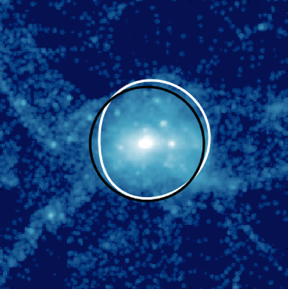
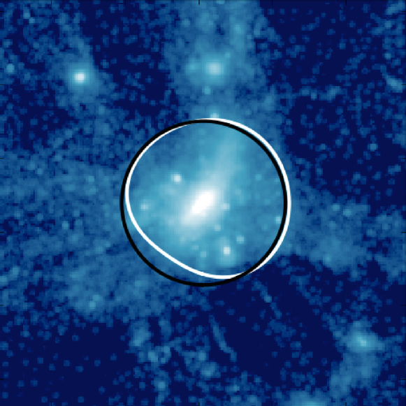
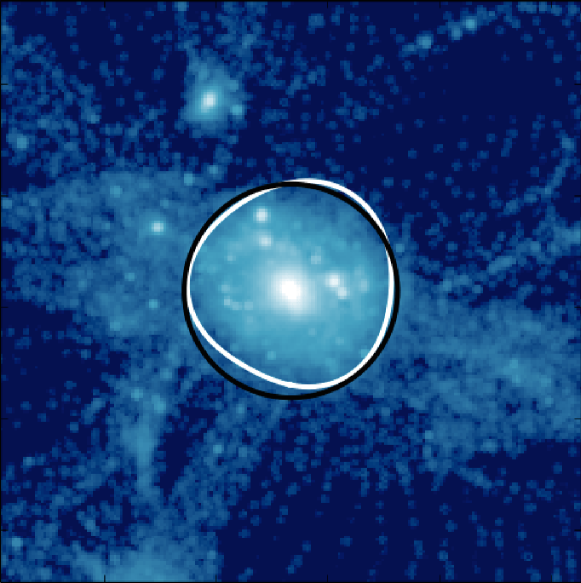
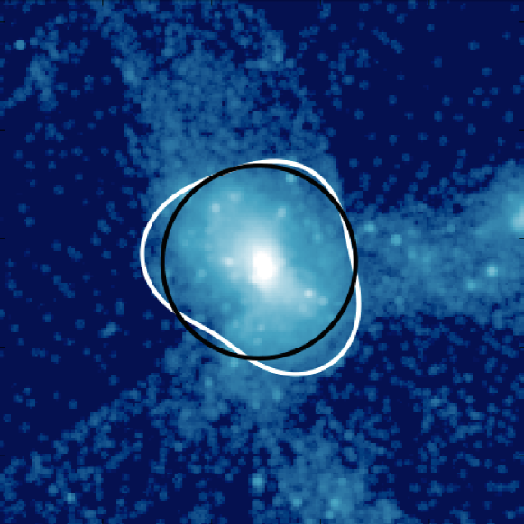
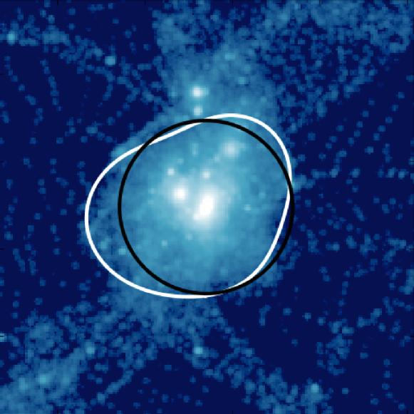
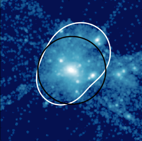
We find that, in general, the identified shells trace the sharp discontinuities in the density field around halos. We illustrate this for six randomly-selected example halos in Figure 2, where the white curves show the cross-sections of the identified shells and the black circles show cross-sections of spheres with radii $R_{\rm sp}$ for those halos. Here $R_{\rm sp}$ corresponds to the volume-equivalent definition given in Equation 7. While we found that this type of simple visual inspection proved to be very effective in identifying ineffective filtering algorithms and parameter sets, it is necessarily a qualitative test and cannot provide a quantitative error estimate.

In our second test, we compare the values of $R_{\rm sp}$ measured by Shellfish to halos which have an unambiguous steepening in their profiles relative to the asymptotic high-$R$ NFW slope due to the splashback shell. Shellfish is unambiguously incorrect for any halos where it measures $R_{\rm sp}$ outside of this steepening region. The difficulty with this test is that is that it is hard to programmatically detect the extent of this steepening region in a robust way. Additionally, large substructure and dense filaments can create steepening regions in the outskirts of host halos which appears similar to the steepening caused by the splashback shell, but occurs in the wrong locations. For these reasons, we resort to manual inspection of halos to perform this test.

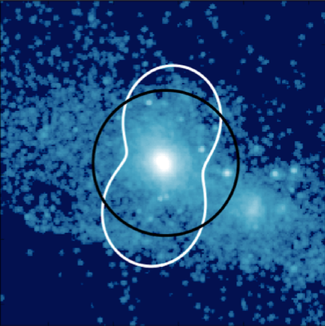
We inspected the outer profiles of roughly 5,000 $z=0$ halos with $N_{\rm 200m}>50,000$ and identified 906 which had a clear steepening of the density profile in their outskirts and did not have a significant subhalo presence in that region. We then identified the starting and ending radii that bracketed the steepening region of each of these halos, $R_{\rm start}$ and $R_{\rm end}$, by eye. We then compared these radial ranges to $R_{\rm sp}$ calculated through Equation 7. We found that only four halos had $R_{\rm sp}$ measurements outside of the ranges measured from the profiles, corresponding to a minimum failure rate of $\approx 0.5\%$. $R_{\rm start}$ and $R_{\rm end}$ can span a wide range of radii (see, e.g., Figure 7 and Figure 16), so this test is not effective at catching $\approx 20\%$ errors. This test is chiefly sensitive to catastrophic failures, which we found could be as common as $25\%$ for poorly constructed filtering algorithms or improperly set parameters. Figure 4 shows an example of a typical catastrophic failure. In this case, there is no strong feature in the surrounding density field which forces Shellfish to generate an unphysical shell. Achieving a low failure rate on this test is a necessary, but not sufficient, condition for any accurate splashback-measuring code.

Figure 4.— A density slice around one of the halos which fails the second test described in section 3 (i.e. a “catastrophic failure”). The image dimensions and the meanings of the white and black curves are identical to those in Figure 2. We found that these halos can be very common for improperly calibrated filtering algorithms, but when the parameters shown in Table 2 are used, these halos make up only $\approx 0.5\%$ of our total halo population.

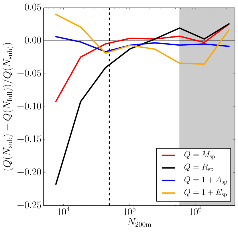
As a third test, we also carried out a convergence study of the shell properties defined in Equations 7 - 11 with respect to the number of dark matter particles within a halo, $N_{\rm 200m}$. These were performed by generating a representative sample of halos and fitting two Penna-Dines shells to each of them. The first shell is calculated using only one eighth of the halo’s particles and the second is calculated using all the halo’s particles. We use the notation that the number of particles in subsampled halos is $N_{\rm 200m}/8=N_{\rm sub}$, and that the number of particles in fully sampled halos is $N_{\rm 200m}=N_{\rm full}$. The results of this test are shown in Figure 3.

Figure 3 shows that for $N_{\rm 200m}>50,000$, the systematic error due to particle count in $M_{\rm sp}$ is at the per cent to sub per cent level, and that the error in $R_{\rm sp}$, $1+E_{\rm sp}$, and $1+A_{\rm sp}$ in the same range is at the few per cent level. The shaded region in Figure 3 indicates bins in which our simulation suite produced two or fewer halos. Figure 3 indicates that to identify splashback shells reliably, halos need to be resolved with at least $5\times 10^{4}$ particles. It is not clear to what extent there is a second order trend in radius after the first order convergence at $N_{\rm 200m}$. It would not be unreasonable to see a trend of this type: as $N_{\rm 200m}$ increases, Shellfish may be able to resolve and fit smaller scale features in halos which could result in small changes in volume. For this reason, we cannot yet rule out that there is a systematic $\lesssim 5\%$ trend with mass for $R_{\rm sp}$.

3.1. Comparison to Particle Trajectories

As a fourth test of the algorithm, we inspect the trajectories of individual particles near the splashback shell. Particles near the correctly identified splashback shells can be expected to be either infalling for the first time or to be at the apocenter of their first orbit. Trajectories of the infalling particles should be roughly perpendicular to the shell locally and should not show any deflection when crossing the shell. The trajectories of the particles that have orbited through the halo should show a sharp turnaround at the shell location. The relative fractions of particles of these two types will depend on the mass accretion rate of each specific halo, but the apocenters of particles of the second type should coincide with the identified splashback shell. Given that our algorithm does not use any information about particles trajectory, this test is a useful independent check on whether our algorithm identifies shells corresponding to the actual outermost apocenters of particle orbits.

To perform this test on a target halo, we first use Shellfish to identify a splashback shell around the halo at some redshift $z_{1}>0$. We then find all particles within some small distance $\delta$ of this shell and track their trajectories through a redshift range $z_{0}<z_{1}<z_{2}$.

The results of such a test are shown for four representative clusters with $M_{\rm 200m}\approx 10^{14}h^{-1}\ M_{\odot}$ from the L0250 simulation in Figure 5, where we used $\delta=R_{\rm 200m}/50$, $z_{0}=0.32$, $z_{1}=0.13$, and $z_{2}=0$. The location of the particles at $z=z_{1}$ is shown by red points. The trajectories of particles from $z_{0}$ to $z_{1}$ are shown as red curves and the trajectories from $z_{1}$ to $z_{2}$ are shown as yellow curves. Infalling particles have red curves pointing outside of the halo and yellow curves pointing inside the halo. Particles moving outwards have reversed colors: yellow curves pointing to the outside and red curves pointing to the inside. Particles at their apocenters will have both curves pointing to the inside.

Figure 5.— Trajectories for particles during the redshift interval $z\in[0.32,0]$ near the splashback shell of four clusters from the L0250 simulation with $M_{\rm 200m}\approx 10^{14}h^{-1}\ M_{\odot}$ identified at $z_{1}=0.13$. Each figure shows a slice through the density field in a region centered on the halo with a width of $5R_{\rm 200m}$ and a depth of $R_{\rm 200m}/5$. Every particle in this slice located within $R_{\rm 200m}/50$ of the splashback shell identified by Shellfish at $z_{1}=0.13$ is shown as a red point. The trajectory of each particle during the redshift interval $[0.31,0.13]$ is shown by red line, while the trajectory during the redshift interval $[0.13,0]$ is shown by yellow lines. See section 3.1 for details.

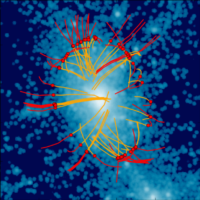
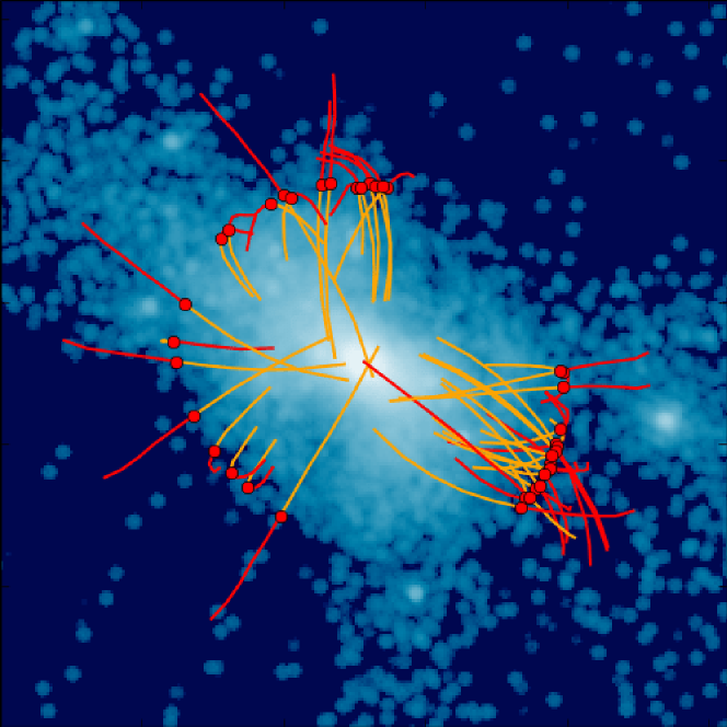
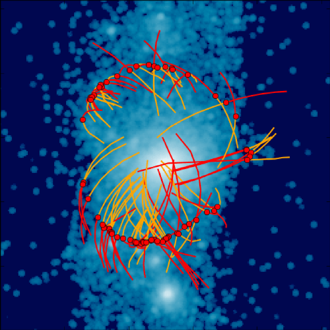
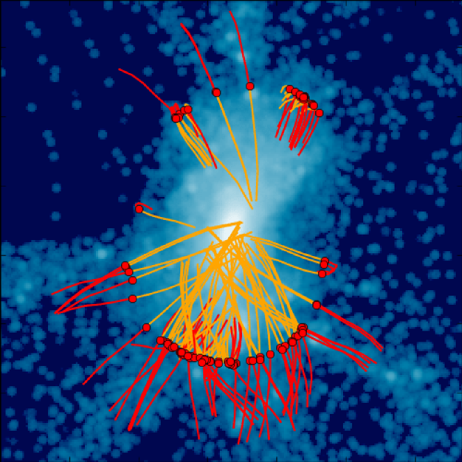
Figure 5 shows that for the cluster-sized halos shown, most particles around the splashback shell are infalling, as can be expected for rapidly accreting halos. At the same time, there is a fraction of particles that exhibit a sharp turnaround near the identified splashback shell: i.e., the apocenters of their orbit coincide with the splashback shell identified from the density field.

Figure 5 does show several trajectories in the southern portion of the halo which travel outside the identified shell. It is not clear whether this is because Shellfish was unable to identify the correct splashback shell due to the high-density filament or whether those particles were perturbed from their orbits in later time steps by the nearby subhalo. Such trajectories, however, are a small fraction of the total.

We have carried out such visual inspection of trajectories for a large number of halos and found results qualitatively similar to those shown in Figure 5. This indicates that our algorithm is reliably picking out splashback shells that coincide with the most distant apocenters of particle orbits. This analysis has been confirmed by comparison with an alternative splashback-measuring code, Sparta, which showed that the radii measured by Shellfish correspond to high-percentile moments of a halo’s apocenter distribution (Diemer et al., 2017).

4. Results

4.1. Sample Selection

To analyze the properties of splashback shells identified using our algorithm we construct a sample of halos drawn from the halo catalogs of all the simulations listed in Table 1. Based on the convergence test results reported in section 3 (see Figure 3), we select halos with $N_{\rm 200m}>50,000,$ so that shell properties are converged to the level $\lesssim 5\%$. We also restrict the maximum mass of halos drawn from the smaller box simulations so that the $\Gamma_{\rm DK14}$ distribution of the largest halos in those simulations is similar to that of halos of the same mass in the larger boxes. This limit is imposed because small box size may limit the mass accretion time of the largest halos, as evolution becomes nonlinear on scales comparable to the box size. The mass ranges sampled by each box are given in Table 1.

With these mass limits in place, we construct the halo sample for analysis by subsampling all host halos within the mass range of each box in such a way as to obtain a uniform distribution of halos in both $\log M_{\rm 200m}$ and $\Gamma_{\rm DK14}$. This procedure is repeated for $z=0$, $z=0.5$, $z=1$, and $z=2$, resulting in a total sample sizes of 1095, 1198, 846, and 467 halos, respectively.

4.2. Comparison With Stacked Radial Density Profiles

Figure 6.— Comparison between the distribution of $R_{\rm sp}/R_{\rm 200m}$ values measured by Shellfish to the prediction of stacked density profile analysis at $z=0.5$. The black curve shows the best fit to location of steepest slope in the stacked density profiles as a function of accretion rate, $\Gamma_{\rm DK14}$. We use the parameterization for this fit reported in More et al. (2015). The blue points show Shellfish $R_{\rm sp}/R_{\rm 200m}$ measurements for individual halos, the blue curve shows the median measurement, and the blue contours show the 68% envelope. The Shellfish curve differs from stacked profiles in both amplitude and shape, becoming $\approx$30% larger for halos with $\Gamma_{\rm DK14}>4$. A qualitatively similar difference can be seen at all redshifts. We argue that this difference is due to stacked profiles splashback measurements being artificially biased inwards by massive subhalos in section 4.2.

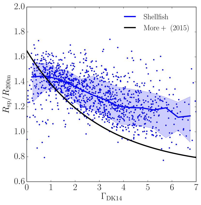
Figure 6 presents a comparison between the distribution of $R_{\rm sp}/R_{\rm 200m}$ values measured by Shellfish and the predictions of stacked profile analysis as a function of accretion rate. In particular, we choose to compare against the $\Gamma_{\rm DK14}$ vs. $R_{\rm sp}/R_{\rm 200m}$ fit reported in More et al. (2015). We have chosen $z=0.5$ for illustration in this figure, because the $z=0.5$ halo sample contains a good mix of well-converged, high particle-count halos which become more abundant as redshift decreases, and halos with large accretion rates, which become more abundant as redshift increases.

The figure shows that at $\Gamma_{\rm DK14}\lesssim 1.5$ our algorithm estimates splashback radii similar to those from stacked profiles, while for $\Gamma_{\rm DK14}\gtrsim 1.5,$ Shellfish estimates progressively larger $R_{\rm sp}$ values compared to the values from the stacked profiles. The discrepancy in $R_{\rm sp}/R_{\rm 200m}$ is $\approx 30\%$ for $\Gamma_{\rm DK14}\approx 4$. This discrepancy exists at all redshifts.

Given that the tests presented in section 3 indicate that our code identifies splashback shells reliably and estimates their properties to better than $5\%$ accuracy at the resolution level shown in Figure 6, it is highly unlikely that the discrepancy is due to any issue of our algorithm. In particular, a systematic overestimation of $R_{\rm sp}$ by 30% would be immediately apparent in the visual comparison of the identified splashback shells and the underlying density field. Instead, we find a good agreement in such comparisons. Additionally, we were able to independently reproduce the results of More et al. (2015) using the halo sample described in section 4.1. Thus, the discrepancy shown in in Figure 6 is the real difference between the two methods.

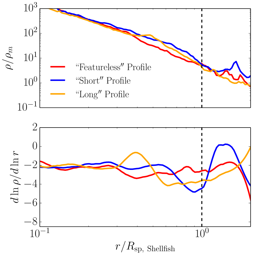
To better understand the origin of this difference, we visually inspected the radial density profiles of all the halos in our sample and classified them into one of three qualitative classes. First, we flagged every halo as either containing a visually distinct steepening region in its outskirts or as containing no such region. Halos of the latter type we classify as “featureless”-type profiles. The red curve in Figure 7 is an example of such a halo.

The remaining halos contain distinct regions in the density profiles where the logarithmic slope steepens considerably over a limited range of radii. For these halos we visually identify the starting radii, $R_{\rm start}$, and ending radii, $R_{\rm end}$ of their respective steepening regions. We find that almost all such halos separate neatly into one of two classes: 1) halos which have relatively sharp and narrow steepening regions that closely correspond to the radial range of the splashback shell found by Shellfish for that halo; and 2) halos which have a relatively shallow and wide steepening region with an $R_{\rm start}$ value significantly smaller than the minimum radius of the shell found by Shellfish. We refer to halos of the first type as “short”-type profiles and halos of the second type as “long”-type profiles, respectively. The blue and yellow curves in Figure 7 are examples of these two types of profiles, respectively. The number of halos is roughly similar in the three classes of “featureless”, “short”, and “long” profile types, but the exact fractions of halos in each class changes with accretion rate and with mass.

We find that when we derive splashback radii from the stacked density profiles using only halos of the short and featureless types, the difference from the median $R_{\rm sp}$ measured by Shellfish decreases to $\lesssim 5\%$ at high $\Gamma_{\rm DK14}.$ This is not surprising, given that we noted that the steepening range in the short-type profiles is consistent with the radial range of the splashback shells derived by Shellfish, but demonstrates that the difference in $R_{\rm sp}$ is due almost entirely to the effect of the halos with the long-type profiles on the stacked density profile.

Our analysis shows that the steepening region in the density profiles of long-type halos is not caused by the splashback shell, but by the presence of massive subhalos. Specifically, visual inspection of the density fields of long-type halos generally reveals that no portion of the splashback shell can be found as far inwards as $R_{\rm start}$ for these halos. Instead, we almost always find that a massive subhalo is present at $R\approx R_{\rm start}$ for these halos. Thus, the steepening region is associated with the presence of subhalo, not the splashback. Given that subhalos in different halos with the same accretion rate will be located at different $R$, the combined effect of the massive subhalos on the stacked profile is to “wash out” the signature of the splashback shell and to bias the start of the steepening region to smaller radii.

Thus, halos with no massive subhalos in the outskirts have the short-type profiles, while those that do have such subhalos have long-type profiles. Halos that either have large neighboring halos outside their splashback shells or which exist in dense filaments have the steepening due to splashback shell erased completely and thus have featureless-type profiles. The expectation is then that if contribution of massive subhalos is removed from the density profiles the $R_{\rm sp}$ derived from the stacked density profiles should be consistent with the values estimated by Shellfish. We demonstrate that this is the case in the next subsection.

4.3. Angular Median Density Profiles of Halos

Figure 7.— Comparison between spherically averaged radial density profiles (Figure 7) and the angular median density profiles described in 4.3 (Figure 7). The top panels show density and the bottom panels show logarithmic slope after the density profiles have been smoothed with a fourth-order Savitzky-Golay filter with smoothing windows a third of a decade wide. Both density and slope profiles have had their radii normalized by $R_{\rm sp}$ as measured by Shellfish. The three halos are chosen to be representative of the three qualitative classes of halo profiles we identified in section 4.2. Because angular median profiles are designed to remove interfering substructure, they have deeper and more well-defined points of steepest slope. The level of agreement between the radius of steepest slope of the angular median profiles shown here and the $R_{\rm sp}$ values derived by Shellfish is typical.

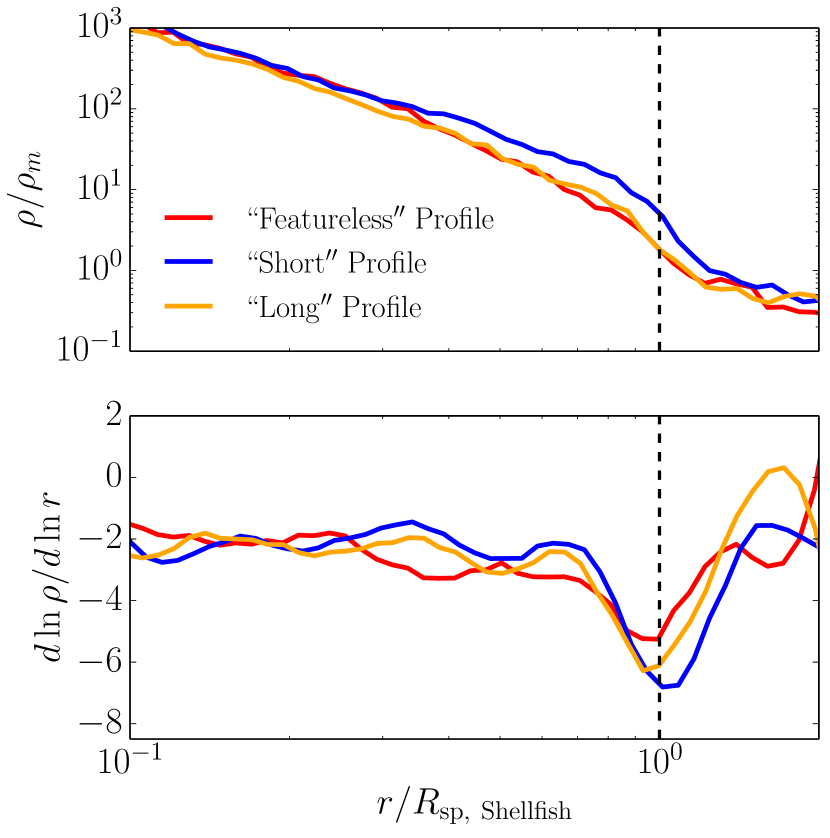
There are many possible ways of mitigating the contribution of subhalos to the density profiles of their host halos. We choose one of the simplest methods for doing this, one which does not rely on the availability of robust subhalo catalogs, and which could, in principle, be adapted for use on observed galaxy clusters. The idea is to construct density profiles using the median estimate of density in each radial shell instead of the mean density. A similar approach has been used in the analysis of the gas distribution in clusters (Zhuravleva et al., 2013).

Namely, we split each radial shell of the density profile into $N$ solid angle segments, e.g., using a two-hemisphere variation on the algorithm described by Gringorten & Yepez (1992), or the HEALPix pixelation algorithm (Górski et al., 2005). We then estimate density, $\rho_{i}(r),$ for each segment $i$ and construct the halo density profile by taking the median of these densities in each radial shell, $\rho_{\rm med}(r)={\rm med}\left[\rho_{i}(r)\right]$. This approach is based on the basic intuition that subhalos are generally much smaller in extent than the host and thus contribute to a fraction of the solid angle in a given radial shell, while most of the solid angle will be dominated by the diffuse matter of the host halo. The median density then will estimate the density of that diffuse component and will be largely insensitive to the outlier solid angle segments associated with massive subhalos.

Figure 7 shows comparisons between usual spherically averaged mean density profiles, $\rho(r),$ and angular median density profiles $\rho_{\rm med}(r)$ for three representative halos of the different classes described in section 4.2. The comparison of the profiles in the two panels of the figure shows that the angular median profiles of the halos are much more similar to each other than the mean profile. Unlike the mean density profiles, which have very different shapes, the angular median density profiles all behave similarly: there is a narrow, sharp steepening region in the logarithmic profile centered on the radius that Shellfish reports as $R_{\rm sp}.$ Thus, the diversity of profile types noted in 4.2 is largely absent for profiles of this type. We also note that the point of steepest slope in angular median profiles is significantly sharper than it is in mean profiles. Thus the signature of the splashback shell is easier to detect when halos are analyzed in this way.

To compare $R_{\rm sp,shell}$ measured by Shellfish to $R_{\rm sp,med}$ derived from the individual angular median profiles, we follow the procedure described above for every halo in the sample described in section 4.1. We use 50 solid angle segments per halo with 30 logarithmically-distributed radial bins per decade. This relatively coarse spacing is needed to make up for the fifty-fold loss in number statistics and has a non-trivial impact on the maximum fidelity of our angular median profiles: the width of every bin is 8% of the radius at which is occurs. Once the median profile is computed from these segments, we apply a Savitzky-Golay smoothing filter with a window size comparable to the characteristic radial width of the regions where profile slope steepens quickly. We set the window size to a $0.33$ dex with the caveat that other reasonable choices, such as a sixth of half of dex, can induce systematic changes to the mean $R_{\rm sp,med}$ of a halo population of $\approx 5\%$. Thus, the population statistics on $R_{\rm sp,med}$ cannot be trusted to accuracies smaller than 5% regardless of any additional statistical error bars, and that individual $R_{\rm sp,med}$ values measured this way cannot be measured more accurately than 13%, regardless of additional profile noise. We leave more nuanced accuracy analysis on this method to a future work, but note that this level of accuracy is sufficient for our purposes, which is merely to test whether reducing effect of subhalos on the radial profiles results in $R_{\rm sp}$ estimates which are qualitatively consistent with the results of Shellfish.

Figure 8.— Comparison between the mean $R_{\rm sp}/R_{\rm 200m}$ values measured by Shellfish and by the angular median profile method described in section 4.3. The left panel shows measurements made by the two methods for different $\Gamma_{\rm DK14}$ and $M_{\rm 200m}$ bins at $z=0.5$. Shellfish measurements are shown as circles on the left side of their respective $\Gamma_{\rm DK14}$ bins, and angular median profile measurements are shown as triangles on the right side of their respective $\Gamma_{\rm DK14}$ bins. Error bars represent only the bootstrapped error on the mean and do not account for known systematic uncertainty in the angular median profile method (see section 4.3). The right panel shows the median value of $R_{\rm Shellfish}/R_{\rm median}-1$, for every halo in our sample at $z$ = 0, 0.5, 1, and 2. The dashed blue lines show the shape of this curve when the angular median profile’s Savitzky-Golay window width is varied to the edges of its physically reasonable value range to give a sense of the systematic variability in this method (see section 4.3). These two figures illustrate that when large subhalos are removed from the density profiles of halos, the location of the point of steepest slope becomes consistent with the value of $R_{\rm sp}$ measured by Shellfish. They also illustrate that there is a non-trivial disagreement between the two methods for very small $\Gamma_{\rm DK14}$.

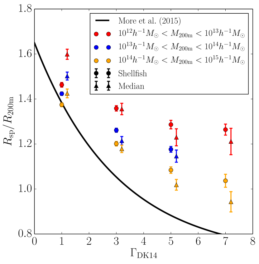
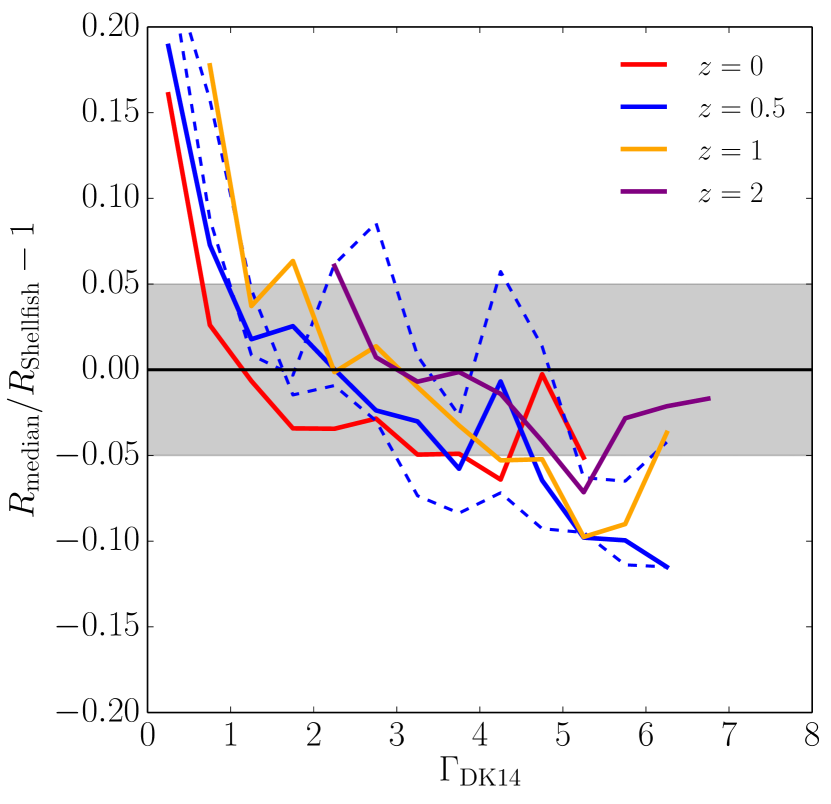
We compare the $M_{\rm 200m}$ and $\Gamma_{\rm DK14}$ trends between $R_{\rm sp,shell}$ and $R_{\rm sp,med}$ for our $z=0.5$ halo sample in Figure 8 and see fairly good agreement. The high $\Gamma_{\rm DK14}$ disagreement has dropped from $\gtrsim 30\%$ to $\approx 5\%.$ This is consistent with the known systematic uncertainties in both methods and confirms that the high $\Gamma_{\rm DK14}$ disagreement with the estimates of the splashback radius from the stacked mean density profiles is due to the bias introduced into these profiles by massive subhalos.

At the same time, at $\Gamma_{\rm DK14}\lesssim 0.5$ there is $\approx 15\%$ disagreement between $R_{\rm sp}$ derived from the stacked angular median profiles and the median measurements of Shellfish. In principle, this difference could be caused by either the angular median profile method or Shellfish, but comparison against another splashback-measuring code, Sparta, which explicitly tracks particle orbits to find their apocenters, shows tight agreement with Shellfish at $\Gamma_{\rm DK14}>0.5$ and a level of discrepancy comparable to that seen for angular median profiles at $\Gamma_{\rm DK14}<0.5$. An extended discussion on how these two methods compare against one another can be found in Diemer et al. (2017).

It is not surprising that the splashback shell is difficult to measure at these accretion rates. At $z=0$, pseudo-evolution causes static NFW halos with $c_{\rm vir}\gtrsim 7$ to report $\Gamma_{\rm DK14}>0.5$ purely due to the cosmological evolution of $\rho_{\rm m}$ (Diemer et al., 2013b). This means that the majority of halos with accretion rates this low must be actively losing particles in order to offset their illusory accretion rates caused by pseudo-evolution. This particle loss is typically caused by dense environments, either because the halo is embedded in a massive filament feeding a cluster or because it is about to merge with a larger halo.

For this reason we believe that our algorithm should not be used to measure halos with $\Gamma_{\rm DK14}<0.5$ unless $\gtrsim 15\%$-level systematic errors are acceptable. We exclude such halos from all subsequent analysis. This is an aggressive cut for Milky Way-sized halos at low redshifts, where $20\%$ of halos have $\Gamma_{\rm DK14}<0.5$. The cut is less severe for halos in all other mass bins and at all other redshifts, affecting less than $5\%$ of halos in all such parameter slices. Clusters and high redshift halos in particular are almost completely unaffected by this cutoff.

4.4. The Relationship Between Mass, Accretion Rate, and Splashback Radius

Figure 9.— Comparison between our fit and Shellfish’s measurements of $R_{\rm sp}/R_{\rm 200m}\equiv\tilde{R}_{\rm sp}(\Gamma_{\rm DK14},\nu_{\rm 200m},z)$. The thick lines represent the median value of $R_{\rm sp}/R_{\rm 200m}$ in each $\Gamma_{\rm DK14}$ bin and the shaded regions indicate the 68% errors on those medians, as determined by bootstrapping. The thin lines show the median of the distribution given by Equations 12 -14 evaluated at the median $\nu_{\rm 200m}$ value within the corresponding $\nu_{\rm 200m}$ bin.

Figure 10.— Comparison between our fit and Shellfish’s measurements for $M_{\rm sp}/M_{\rm 200m}\equiv\tilde{M}_{\rm sp}(\Gamma_{\rm DK14},\nu_{\rm 200m},z)$. The visualization scheme is identical to the one used in Figure 10, with the thin line corresponding to the median of the distribution given by Equations 15 and 16. Note that unlike the fit displayed in Figure 9, our $\tilde{M}_{\rm sp}$ has no $\nu_{\rm 200m}$ dependence, so only a single thin line is plotted. There are several important caveats to this fit, which we discuss in section 4.5.

Figure 11.— Comparison between the $\tilde{M}_{\rm sp}$ median and $68\%$ contours for our data and our fit given by Equations 15 and 16 at $z=0$. This Figure was made to emphasize the weaknesses in our $\tilde{M_{\rm sp}}$ fit and shows an $\approx 2\%-4\%$ overestimation of the median at high $\Gamma_{\rm DK14}$ and a similar overestimation of the logarithmic scatter, $\sigma_{\rm dex}$. An extended discussion of this Figure can be found in section 4.5.

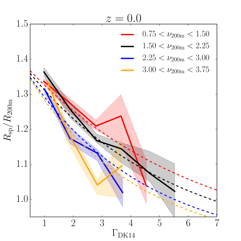
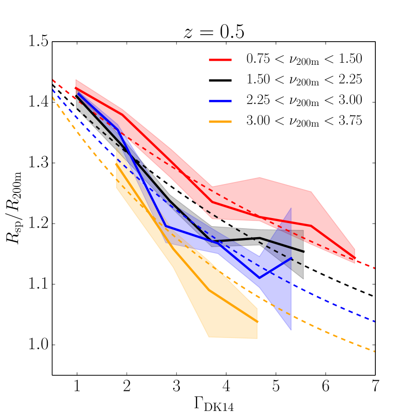
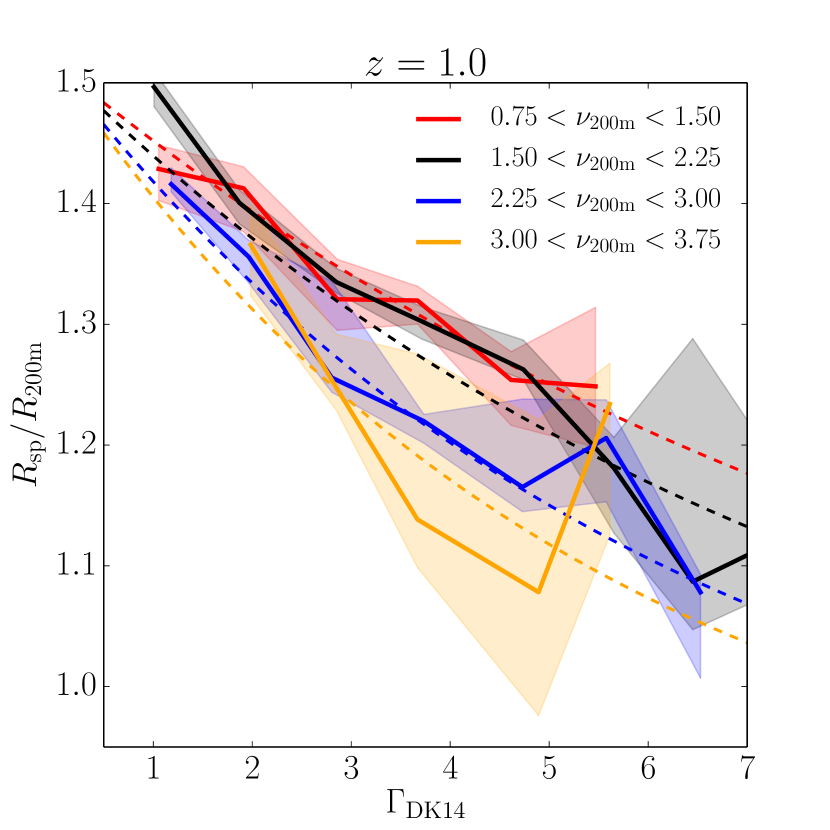
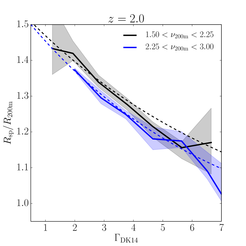
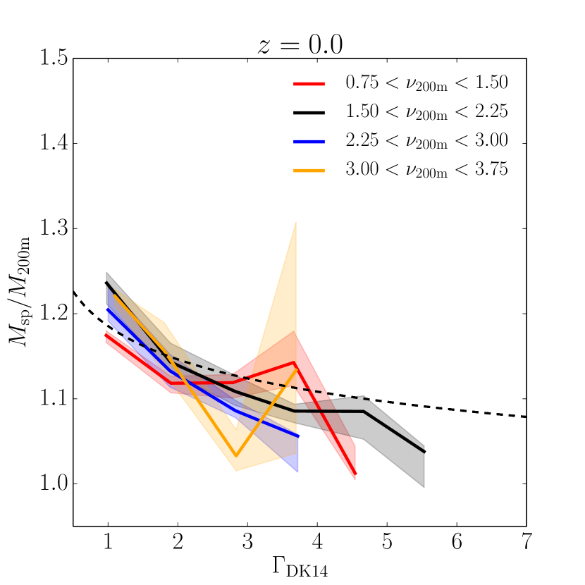
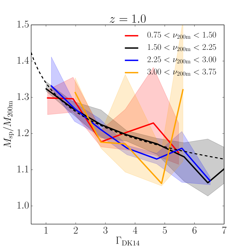
One of the key results obtained by previous analyses of splashback shells using stacked radial density profiles (Diemer & Kravtsov, 2014; More et al., 2015, 2016; Adhikari et al., 2016) is the dependence of the splashback radius in units of the $R_{\rm 200m}$ on the mass accretion rate $\Gamma_{\rm DK14}$ (see Equation 2): halos with larger accretion rates have smaller values of $R_{\rm sp}/R_{\rm 200m}\equiv\tilde{R}_{\rm sp}$. In this section we present the result of fits to $\tilde{R}_{\rm sp}$ using the measurements from Shellfish.

Specifically, we fit the following log-normal distribution to $\tilde{R}_{\rm sp}$ as a function of $\nu_{\rm 200m},$ $\Gamma_{\rm DK14},$ and $\Omega_{m}$:

$$P(\tilde{R}_{\rm sp}) \propto\exp(-\log_{10}^{2}(\tilde{R}_{\rm sp}/R_{\rm med})/2\sigma_{\rm dex}^{2}),$$ (12)

$$R_{\rm med} =(R_{0}\Omega_{m}+R_{1})\exp{(\alpha\Gamma_{\rm DK14})}+A,$$ (13)

$$\alpha =\eta_{0}\Omega_{m}^{2}+\eta_{1}\Omega_{m}+\eta_{2}+\xi\nu_{\rm 200m}.$$ (14)

Here $R_{0}$, $R_{1}$, $A$, $\xi$, $\eta_{0}$, $\eta_{1}$, and $\eta_{2}$ are fit parameters.

As discussed above, our sample only includes halos with $\Gamma_{\rm DK14}>0.5.$ We fit the functional form given by Equations 12–14 using an implementation of the affine-invariant Markov Chain Monte Carlo sampling algorithm of Goodman & Weare (2010). We also adopt a Heaviside prior on the logarithmic scatter, $\sigma_{\rm dex},$ to prevent it from becoming non-positive.

We find that the best fit parameters are

$$R_{0} =0.2181, \eta_{0} =-0.1742,$$

$$R_{1} =0.4996, \eta_{1} =0.3386,$$

$$A =0.8533, \eta_{2} =-0.1929,$$

$$\xi =-0.04668, \sigma_{\rm dex} =0.046.$$

The resulting function is plotted against our data in Figure 9.

It is interesting that the radii estimated by Shellfish exhibit a strong dependence on both mass accretion rate and peak height. This trend can also be seen in other methods for measuring individual splashback shells around halos, such as the median angular profile method described in section 4.3 and the apocenter-based splashback-measuring code Sparta (Diemer et al., 2017). The trend cannot be attributed to convergence trends because all halos used in the sample have $N_{\rm 200m}$ above the convergence limit of $5\times 10^{4}$ found in section 3 and because the mass bounds given in Table 1 restrict the halos in our sample to a single decade in particle count.

Previous estimates from stacked density profiles only found a strong dependence on $\Gamma_{\rm DK14}$, while a $\nu_{\rm 200m}$ dependence was either not apparent or weak (e.g., More et al., 2015). The $\nu_{\rm 200m}$ dependence is also not predicted in the collapse models of isolated peaks (e.g., Adhikari et al., 2014), even though they successfully predict a $\Gamma_{\rm DK14}$ dependence. The origin of the $\nu_{\rm 200m}$ dependence and the seeming discrepancy with the collapse model is not clear. Additionally, although we have made an empirical argument that stacked profiles are biased by massive subhalos, we do not yet propose a physical picture for why this bias should also erase or decrease trends with $\nu_{\rm 200m}$.

4.5. Splashback Shell Masses

In contrast to overdensity-based halo definitions, $M_{\rm sp}$ and $R_{\rm sp}$ are independent (albeit correlated) quantities. For this reason we do not fit the same functional form to both $R_{\rm sp}$ and $M_{\rm sp}.$ We fit the following log-normal distribution to $\tilde{M}_{\rm sp}\equiv M_{\rm sp}/M_{\rm 200m}$ as a function of $\Gamma_{\rm DK14}$ and $\Omega_{m}$:

$$P(\tilde{M}_{\rm sp}) \propto\exp(-\log_{10}^{2}(\tilde{M}_{\rm sp}/M_{\rm med})/2\sigma_{\rm dex}^{2}),$$ (15)

$$M_{\rm med} =(M_{0}\Omega_{m}+M_{1})\left(\frac{\Gamma_{\rm DK14}}{\Gamma_{\rm pivot}}\right)^{\alpha_{0}\Omega_{m}+\alpha_{1}}.$$ (16)

Here $\Gamma_{\rm pivot}=3$ is a characteristic pivot value, and $M_{0},$ $M_{1}$, $\alpha_{0}$, and $\alpha_{1}$ are fit parameters.

Using the same procedure described in section 4.4 we obtain the parameters

$$A_{0} =0.192 a_{0} =-0.0781$$

$$A_{1} =1.072 a_{1} =-0.0284$$

$$\sigma_{\rm dex} =0.054$$

The median of this fit is shown in Figure 10. Note that unlike our fit to $\tilde{R}_{\rm sp}$, we do not model $\tilde{M}_{\rm sp}$ as having a $\nu_{\rm 200m}$ dependence because there is not strong evidence for such a trend in our data. This contrasts with the results of Sparta, which did find a strong $\nu_{\rm 200m}$ trend (Diemer et al., 2017). It is currently not clear whether higher quality data would reveal a small mass trend in the Shellfish data as well.

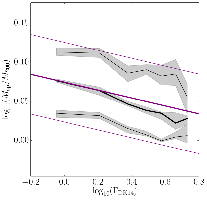
The left panel of Figure 10 shows a deviation between our fit and Shellfish’s measurements at high $\Gamma_{\rm DK14}$ for $z=0$. We investigate this further in Figure 11 which shows the median and 68% contours of the $\tilde{M}_{\rm sp}$ distribution at $z=0$. This Figure shows that although the median of our data is well approximated by a power law, our Bayesian fit reports a shallower slope. This results in a $\approx 2\%-4\%$ overestimation of $\tilde{M}_{\rm sp}$ at high accretion rates for this redshift.

This overestimation is caused by the fact that at high $\Gamma_{\rm DK14}$ $\tilde{M}_{\rm sp}$ follows an skewed log-normal distribution. Since our model assumes a log-normal distribution, our fit’s median is pulled high relative to our data’s median. The offset between the two medians also leads to an overestimation of the logarithmic scatter, $\sigma_{\rm dex}$ by a comparable amount.

Despite this, we deliberately choose not to model the skew for three reasons. The first reason is simplicity: our experiments with explicitly modeling the skew show that it has non-linear dependencies on $\Gamma_{\rm DK14}$ and $z.$ The second reason is that this reduction in simplicity would result in an increase in accuracy for only a small number of halos: high accreting halos at $z=0$ are rare. The third reason is that this effect is comparable to our stated systematic uncertainty in the radii and masses reported by Shellfish, so any subsequent analysis which would reach a qualitatively different conclusion from an improvement in fit modeling is not respecting the known uncertainty in Shellfish shells. Instead, we choose to use an extremely simple model - a power law with log-normal residuals and a linear dependence on $\Omega_{m}$ - and leave more precise modeling to future work.

The skew seen in the the low redshift, high $\Gamma_{\rm DK14}$ has a simple explanation. The scatter in $\tilde{M}_{\rm sp}$ has two sources: the first is the variation in shell sizes which also causes the scatter in $\tilde{R}_{\rm sp}$, the second is the presence or non-presence of high mass subhalos. Since halos with high accretion rates are more likely to have high mass subhalos than halos with low accretion rates, the second effect is particularly important for them. If a halo has a massive subhalo outside of $R_{\rm 200m}$ but inside its splashback shell, $\tilde{M}_{\rm sp}$ is scattered high. If a halo has a massive subhalo inside $R_{\rm 200m}$, both $M_{\rm 200m}$ and $M_{\rm sp}$ increase, so $\tilde{M}_{\rm sp}$ scatters towards 1. When the median of the of the $\tilde{M}_{\rm sp}$ distribution is close to 1, this means that the presence of massive subhalos has the effect of reducing down scatter and increasing upscatter relative to what we would expect from variation in shell sizes alone.

4.6. Splashback Shell Overdensities

We model the distribution of $\Delta_{\rm sp}\equiv 200\tilde{M}_{\rm sp}/\tilde{R}_{\rm 200m}$ by taking the ratios of our mass fit (Equations 15 and 16) and our radius fit (Equations 12 - 14). Because our $\Delta_{\rm sp}$ model is derived from our $\tilde{M}_{\rm sp}$ fit, it is subject to the same caveats discussed in section 4.5. However, because the dynamic range of $\Delta_{\rm sp}$ is larger than that of $\tilde{M}_{\rm sp}$, the affect of a few-percent disparity in masses is minimal.

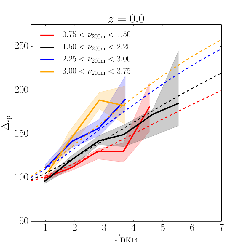
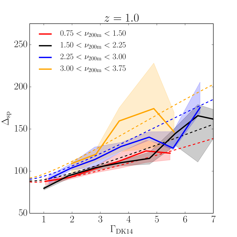
This ratio is shown in Figure 12. Median overdensities range between $\approx$ 70 and $\approx$ 200 with strong dependencies on peak height, accretion rate, and redshift. The most important consequence of these relations is that there is not a single classical overdensity boundary which corresponds to to the splashback shell.

Figure 12.— Comparison between our fits and Shellfish’s measurements for $\Delta_{\rm sp}\equiv 200\tilde{M}_{\rm sp}/\tilde{R}_{\rm 200m}$ using the ratio of our mass and radius fits. The visualization scheme is identical to the one used in Figure 10, with the thin line corresponding to the median of the distribution given by Equations 15 and 16. There are several important caveats to this fit, which we discuss in section 4.5.

4.7. Splashback Shell Shapes

Figure 13.— The asphericity parameter, $A_{\rm sp}$, versus the ellipticity parameter, $E_{\rm sp}$ (defined in Equations. 11 and Equation 10, respectively) for our $z=0$ halo sample. The blue shaded region shows the range of values of these quantities for ellipsoids with different axis ratios. The fact that $A_{\rm sp}$ and $E_{\rm sp}$ of the splashback shells lie above the shaded regions means that the shells have significantly higher surface areas than ellipsoids of similar ellipticity and volume.

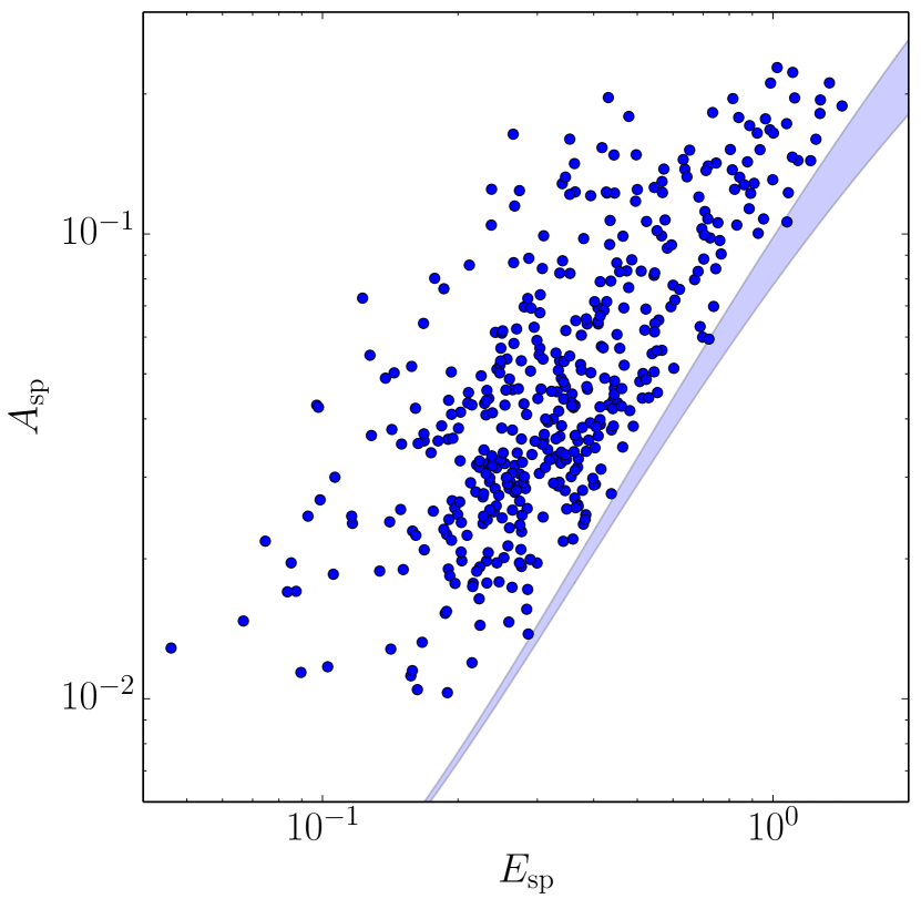
We also investigate the shapes of splashback shells using the asphericity, $A_{\rm sp}$, and ellipticity, $E_{\rm sp}$, parameters defined in Equations 11 and  10, respectively. A plot of these two quantities is shown in Figure 13. The shaded blue region shows the values of these parameters for ellipsoids with different axis ratios. The fact that $A_{\rm sp}$ and $E_{\rm sp}$ for all splashback shells lie above the shaded regions means that the shells are significantly more aspherical than ellipsoids.

We perform checks for correlation between $A_{\rm sp}$, $E_{\rm sp}$ and each of $M_{\rm 200m}$, $\Gamma_{\rm DK14}$, $R_{\rm sp}$, and redshift, but find no evidence of such correlations.

Figure 14.— The correlation function, $\xi(\theta_{\Delta})$, between the major axes of splashback shells and the major axes of total dark matter distribution. The dashed black line shows $\xi(\theta_{\Delta})=0,$ and indicates the level of correlation expected for random alignment.

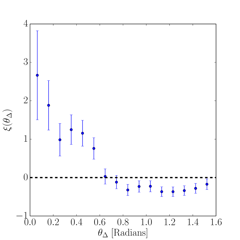
We also calculated the angle $\theta_{\Delta}$ between the major axis of a halo’s splashback shell and the major axis of the underlying dark matter distribution, as reported by the Rockstar halo finder (Behroozi et al., 2013). In Figure 14 we show the correlation function for the angle between these two axes, $\theta_{\Delta}$. We find anti-correlation at high values of $\theta_{\Delta}$ and a high degree of correlation at low values of $\theta_{\Delta},$ indicating that splashback shells are preferentially aligned with major axis of the central dark matter distribution. This is consistent with earlier studies, which have shown that the axis ratios of the matter distribution near the centers of halos tend to be roughly aligned with the axis ratios near the outskirts of halos (Jing & Suto, 2002).

5. Summary and Conclusions

In this paper we presented a new algorithm which identifies the splashback shells around individual halos in simulations. These shells are caused by the caustics formed by matter at the first apocenter of their orbits around the halo and correspond to rapid drops in the density field. Our algorithm relies only on the density distribution within a single simulation snapshot, and is capable of identifying shells with highly aspherical shapes.

We implemented our algorithm in the publicly available code Shellfish and performed extensive tests on the correctness of this code. We performed convergence tests on the splashback shells found by our code and found that above a convergence limit of $N_{\rm 200m}=5\times 10^{4}$, Shellfish can measure properties of splashback shells with $\lesssim 5\%$ systematic error (see Figure 3 and Figure 8) and percent-level stochastic error (see Figure 16). However, we identified a sub-population of halos with low mass accretion rates, $\Gamma_{\rm DK14}\lesssim 0.5$, for which the splashback shell radii estimated by Shellfish are biased low by $\gtrsim 10\%$. We therefore recommend that our code not be used for measurements of splashback shells for halos with $\Gamma_{\rm DK14}<0.5$. This cutoff removes $20\%$ of Milky Way-sized halos at $z=0$ and has a negligible effect on all larger mass scales and all earlier redshift slices.

We presented the first measurements of several basic properties of splashback shells which are summarized below:

1. We confirmed that splashback radii generally decrease with increasing mass accretion rate, as previously found by analyses of stacked halo density profiles. However, we found that the splashback radii found by Shellfish are larger than these earlier estimates by 20%-30% for halos with high accretion rates, $\Gamma_{\rm DK14}\gtrsim 3$. We showed that the estimate of the splashback radius obtained from the stacked density profiles is biased low due to the existence of high-mass subhalos in many of these profiles.

2. We used a simple method, completely independent from Shellfish, for mitigating the effect of substructure on density profiles: the so-called “angular median profile” method. In this method, radial shells are split into solid angle segments with an estimate of density in each segment. The halo density at a given radius is then taken to be the median of all the segments in the corresponding shell. We showed that the effect of subhalos on these profiles is greatly reduced. Moreover, the angular median profiles are more self-similar in their outskirts and exhibit a sharper region of profile steepening (i.e., a much more distinct splashback feature). We showed that the splashback radii estimated from the stacked angular median profiles are in good agreement with the results of Shellfish for halos with $\Gamma_{\rm DK14}\gtrsim 0.5$.

3. We investigated the correlation between splashback radius and mass accretion rate, the scatter around it, and its evolution with redshift. We presented the first evidence that the splashback radius depends not only on accretion rate, but also has a strong dependence on the peak height, $\nu_{\rm 200m}$, with larger $\nu_{\rm 200m}$ halos having systematically smaller $R_{\rm sp}/R_{\rm 200m}$ at a fixed $\Gamma_{\rm DK14}$ and $z$. We found that the scatter of $R_{\rm sp}/R_{\rm 200m}$ around the median at a given accretion rate is significant, exceeding $10\%$. We provided an accurate fit for $R_{\rm sp}/R_{200m}$ and its scatter as a function of $\Gamma_{\rm DK14}$, $\nu_{\rm 200m}$, and $\Omega_{\rm m}$ (see Equations 12-14 and Figure 9). We provided a similar fit for $M_{\rm sp}/M_{\rm 200m}$ (see Equations 15 and 16 and Figure 10). Unlike our fit to $R_{\rm sp}$, there are several minor caveats to our $M_{\rm sp}$ fit, which we discuss in section 4.5.

4. We argued that a single classical overdensity density cannot be used as a model of the location of $R_{\rm sp}$ because the overdensity of splashback shells have a large dynamic range and have strong dependencies on mass, accretion rate, and redshift.

5. We studied the shapes of the splashback shells using an ellipticity parameter, $E_{\rm sp}$, and an asphericity parameter, $A_{\rm sp}$ (defined in Equations 10 and 11, respectively). We showed that splashback shells are generally highly aspherical, with non-ellipsoidal oval shapes being particularly common.

6. We investigated potential correlations between splashback shell properties and other halo properties, but found no significant correlations between $E_{\rm sp}$ and $A_{\rm sp}$ with either mass accretion rate, mass, splashback radius or redshift. However, we did find that the major axes of splashback shells were correlated with the major axis of mass distribution within the inner regions of halos.

This paper is a pilot study of splashback shells of individual halos. Further applications of the algorithm presented here include investigation of alternative classifications of isolated halos and subhalos using the splashback shell instead of the virial radius, investigation of the systematic differences in halo masses and halo mass accretion histories when $M_{\rm sp}$ is compared to $M_{\rm\Delta}$, and a comparisons with other methods for measuring individual splashback shells.

Appendix A An algorithm for fast line of sight density estimates

Figure 15.— An illustration of the UpdateProfiles’ algorithm described in Appendix A. Panel A shows three, $S_{i}$, associated with three dark matter particles around the center of a halo, shown as a solid circle. Panel B shows one of the random planes, $P\in P_{H}$, passing through the halo center and intersections of $P$ with each $S_{i}$. The top and left spheres intersect $P$ while the remaining sphere does not. Panel C shows intersection checks being performed between the 2D intersection, $C_{i}$, of $S_{i}$ and $P$ along a set of lines of sight, $L_{P,i}$, in the plane. Inspection of the angular locations of the edges of the $C_{i}$ shows that only the red lines of sight could intersect them, and thus these spheres contribute to density profiles only along the red lines. This last panel corresponds to the code inside the innermost conditional of the algorithm.

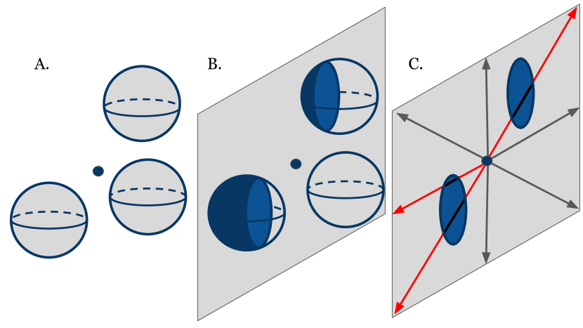
In this Appendix we describe the method our algorithm uses to construct density profiles along a set of lines of sight via the evaluation of Equation 3. Generally, this can be broken up into two steps: first, the set of all spheres which intersect with a particular halo, $H$, is found, and second, for every sphere, $S,$ which intersects with $H$ a procedure UpdateProfiles($S$, $H$) is run, which evaluates a term in Equation 3 corresponding to $S$ for every line of sight in $H$.

In general, the first step is straightforward to perform efficiently. Even rudimentary spatial partitioning (such as breaking the simulation’s particles into $\approx 10^{2}-10^{3}$ spatially coherent segments) results in this step being highly subdominant to the second, making UpdateProfiles the only performance bottleneck of this algorithm. A naive implementation of UpdateProfiles would look like the following:

procedure UpdateProfiles($S$, $H$)

     for each $L$ in $L_{H}$ do

         if $S$ intersects $L$ then

              $R_{\rm enter},$ $R_{\rm exit}$ $\leftarrow$ IntersectionRadii($L$, $S$)

              InsertToProfile($L,$ $\rho_{\rm S},$ $R_{\rm enter},$ $R_{\rm exit}$)

         end if

     end for

end procedure

Here, $L_{H}$ is the set of all line of sight profiles belonging to the halo $H$ and $\rho_{S}$ is the density of the sphere $S.$ The existence of two simple functions has been assumed: IntersectionRadii($L$, $S$) calculates the radii at which the line of sight $L$ enters and exits the sphere $S,$ respectively, and InsertToProfile($L$, $\rho$, $R$, $R^{\prime}$) inserts a rectangular function with amplitude $\rho$ between $R$ and $R^{\prime}$ to the profile corresponding to the line of sight $L$.

Because UpdateProfiles performs an intersection check for every line of sight in $L_{H}$, the asymptotic cost of this approach is $O(|L_{H}|)$. Because $|L_{H}|$ is on the order of 10⁴ for the parameter set used in this paper, this leads to a large number of expensive intersection checks being performed for every particle, with the vast majority of these checks failing.

We take an alternative approach that allows us to avoid performing explicit calculations on any line of sight which does not intersect $S.$ We require that lines of sight exist within a set of planes, $P_{H}$, that $|P_{H}|\ll|L_{H}|,$ and that lines of sight are oriented in uniformly-spaced “rings” within their respective planes. This strong geometric restriction allows for two optimizations: first, intersection checks are performed on entire planes before any calculations are done on individual lines of sight, and second, we calculate the angle subtended by $S$ in intersected planes, which allows us to find the exact set of lines of sight intersected by $S$ in the plane. Concretely, our approach is:

procedure UpdateProfiles^′($S$, $H$)

     for each $P$ in $P_{H}$ do

         if $S$ intersects $P$ then

              $C$ $\leftarrow$ SliceSphere($S$, $P$)

              $\theta_{\rm low}$, $\theta_{\rm high}$ $\leftarrow$ AngularRange($P$, $C$, $H$)

              $i_{\rm low}$, $i_{\rm low}^{\prime}$ $\leftarrow$ ProfileIndices($\theta_{\rm low}$)

              $i_{\rm high}$, $i_{\rm high}^{\prime}$ $\leftarrow$ ProfileIndices($\theta_{\rm high}$)

              for each $i$ in [$i_{\rm low}$, $i_{\rm high}^{\prime}$] do

                  $R_{\rm enter}$, $R_{\rm exit}$ $\leftarrow$ IntersectionRadii($L_{P,i}$, $S$)

                  InsertToProfile($L_{P,i},$ $\rho_{\rm S},$ $R_{\rm enter},$ $R_{\rm exit}$)

              end for

         end if

     end for

end procedure

Here, $P_{H}$ is the set of all planes of profiles belonging to the halo $H$ and $L_{P,i}$ is the $i^{\rm th}$ profile within the profile ring corresponding to the plane $P$. Here, the existence of several simple functions has been assumed: SliceSphere($S$, $P$) returns the circle created by slicing the sphere $S$ by the plane $P$; AngularRange($P$, $C$, $H$) returns two angles specifying the angular wedge within the plane $P$ which the circle $C$ subtends relative to the center of the halo $H$; and ProfileIndices($\theta$) returns the indices of the two nearest profiles to the angle $\theta,$ with the profile corresponding to the lower angle being returned first. For ease of reading, the pseudocode which would handle the periodicity of angles at $\theta=0\equiv 2\pi$ has been omitted.

This method is illustrated in Figure 15. Panel A shows a collection of spheres collected around a halo center, panel B shows the results of calling SliceSphere on each of these spheres for a particular plane, and panel C shows the profiles (in red) which would recieve intersection checks within the innermost loop of UpdateProfiles^′.

The asymptotic cost of UpdateProfiles^′ is $O(|P_{H}|+I_{H,S})$, where $I_{H,S}$ is the number of profiles in the halo $H$ which intersect the sphere $S$. Since both $|P_{H}|$ and $I_{H,S}$ are multiple orders of magnitude smaller than $|L_{H}|$, this results in a significant increase in performance. In practice we find that the plane intersection checks are subdominant to the cost of the innermost loop.

The method described above is further optimized in several ways:

• If InsertToProfile is implemented naively - by representing profiles as arrays containing $\rho(r)$ and updating every element of the profile which is within the inserted rectangular function - it is the dominant cost of UpdateProfiles^′. To prevent this, we represent our profiles as arrays containing $d\rho(r)/dr$. Since the derivative of a rectangular function is two delta functions, updating the derivative profile only requires updating array elements close to the edges of the rectangular function (note that in the discrete case this requires four element updates: two for each edge). Once UpdateProfiles^′ has been called on every target sphere, each derivative profile is integrated to obtain $\rho(r)$.

• Instead of explicitly performing the 3D IntersectionRadii($L_{P,i}$, $S$), a faster 2D analog is used to find the intersection radii of the projection of $L_{P,i}$ onto $P$ with the circle $C$.

• A successful intersection check between $P$ and $S$ is performed in a way which immediately results in the value that would be returned by SliceSphere($S$, $P$), as these two calculations share many geometric operations.

This algorithm is straightforward to generalize to non-constant density spheres and to density estimates constructed from other geometric solids (most notably tetrahedra), although the publicly released version of Shellfish does not allow access to either feature.

Appendix B Splashback candidate filtering algorithm

The Appendix will outline the filtering algorithm which we qualitatively introduced in section 2.2.3

The first step of constructing the filtering loop is dividing the point distribution into $2^{N_{\rm rec}}$ uniformly spaced angular wedges, for some user-defined $N_{\rm rec}$. We calculate an anchor point for each wedge, which is an estimate of the average location of the splashback shell within that wedge.

The location of the anchor point within the $i^{\rm th}$ wedge is given by

$$R_{{\rm anchor},i},~{}\theta_{{\rm anchor},i}=\textsc{AnchorRadius}(0,~{}i),~{}2\pi\frac{i+0.5}{2^{N_{\rm rec}}}.$$ (B1)

Here, $i$ is zero-indexed and AnchorRadius is the following recursive algorithm:

function AnchorRadius($k$, $i$)

     $\theta_{\rm low}\leftarrow 2\pi\lfloor i/2^{k}\rfloor 2^{k-N_{\rm rec}}$

     $\theta_{\rm high}\leftarrow 2\pi(\lfloor i/2^{k}\rfloor+1)2^{k-N_{\rm rec}}$

     $f\leftarrow$ WedgeKDE($\theta_{\rm low}$, $\theta_{\rm high}$)

     if $k$ = $N_{\rm rec}$ then

         return GlobalMaximum($f$)

     else

         $R_{\rm anchor}\leftarrow$ AnchorRadius($k+1$, $i$)

         maxes $\leftarrow$ LocalMaxima($f$)

         $R_{\rm anchor}^{\prime}\leftarrow$ min${}_{R}\{|R_{\rm anchor}-R|~{}\forall~{}R\in{\rm maxes}\}$

         if $|R_{\rm anchor}-R_{\rm anchor}^{\prime}|~{}<~{}R_{\rm refine}$ then

              return $R_{\rm anchor}^{\prime}$

         else

              return $R_{\rm anchor}$

         end if

     end if

end function

We assume the existence of three simple functions: GlobalMaximum($f$), which returns the global maximum of the function $f$; LocalMaxima($f$), which returns all the local maxima of the function $f$; and WedgeKDE($\theta_{\rm low}$, $\theta_{\rm high}$), which returns a kernel density estimate (KDE) corresponding to the points contained within the wedge with boundaries $\theta_{\rm low}$ and $\theta_{\rm high}$. A KDE is a method for converting a set of discrete points into a continuous density estimate by applying a smoothing kernel to every point. It performs much the same role as a histogram, except that an explicit choice of bin edges is replaced by an explicit choice of the smoothing kernel. For our purposes, the most useful property of a KDE is that it provides a simple way to estimate the point of maximum density. We define our KDE as the function

$${\rm KDE}(r)=\sum_{j}\exp{\left(-\frac{(r-r_{j})^{2}}{2R^{2}_{\rm KDE}}\right)}$$ (B2)

where $R_{\rm KDE}$ is a user-defined smoothing scale, and $r_{j}$ is a set of points.

The intuition behind this approach is that most candidate points in the plane correspond to lines of sight crossing the splashback shell, so the maximum of the $k=N_{\rm rec}$ KDE is a good 0^th order estimate of of its location. Smaller wedges give more refined estimates. But if their estimate deviates too far from the coarser estimates, it’s likely that the region corresponds to a filament or a subhalo.

Once anchor points have been found for each wedge, we fit a cubic interpolating spline to them in the $\theta$ - $R$ plane. This spline is the aforementioned filtering loop. To remove boundary effects, the range of the anchor points is extended to $[-2\pi,~{}4\pi)$ prior to fitting, but the spline is only ever evaluated in the $[0~{}2\pi)$ range. We then remove all points which are further than some distance, $R_{\rm filter}$ from this spline.

This procedure introduces three new free parameters, $R_{\rm KDE}$, $R_{\rm refine}$, and $R_{\rm filter}$. Tests indicate that the final shells are robust to changes in $R_{\rm KDE}$ and $R_{\rm filter}$, as long as they are of the same order of magnitude as $R_{\rm refine}$. For this reason we simplify parameters by requiring

$$R_{\rm KDE}=R_{\rm refine}=R_{\rm filter}=R_{\rm max}/\eta.$$ (B3)

Here $\eta$ is a tunable parameter which dictates how strict the filtering process is. Higher values of $\eta$ are stricter than lower values of $\eta$.

Appendix C Parameter-specific convergence tests

Most of the fiducial values of parameters of our algorithm listed in Table 2 were set using one of the following three approaches, which start with constructing a representative sample of halos and identifying their splashback shells and estimating their properties for a range of values $p_{i}$ for the selected parameter $p$.

1. Many parameters are known to be optimized when taken to either the low value or high value limit, but also decrease the performance of the algorithm as the parameter approaches this limit. In addition to the shells for the $p_{i}$ values, we also fit a shell with $p$ set to some very large value, $p_{\rm limit}$. For each halo we calculate a curve representing the fractional difference between the shells calculated with $p_{i}$ and with $p_{\rm limit}$ for each of the properties defined in Equations 7 - 11. We then set the parameter to the lowest $p_{i}$ which leads to an average fractional error of $\lesssim$ 1%.

2. Some parameters are not optimized in either the low or high value limit. For each halo we construct curves for each of the properties defined in Equations 7 - 11. We manually inspect these curves: if they generally show an unchanging “plateau” for these properties over a wide range of $p_{i}$ values, we set the parameter to an arbitrary $p_{i}$ in the center of the plateau. The existence of a plateau over a wide range of $p_{i}$ indicates that the shell shapes depend only weakly on this parameter.

3. For parameters where method B was attempted but a no wide plateau was found, we incorporate qualitative assessment of the shells into the selection procedure. For a pair of parameter values, $p_{i}$ and $p_{j}$, we visually inspect every halo in the test set, compare the shells produced by both values to the underlying density field, and select one of the two as a qualitatively better fit. Once this has been completed for every halo, we label the parameter value with more successful fits as the better value. This allows us to construct an fitness ordering on all the values of $p_{i}$. We then select the maximally fit parameter. In principle, this methodology could lead to researcher-dependent results, but for the three parameters where we used this method, the optimal value was not ambiguous.

The specific methods we used to set each algorithm parameter are listed in Table 2. In all cases the halo sample is divided into $M_{\rm 200m}$-selected and $\Gamma_{\rm DK14}$-selected subsets to test for parameter dependence on halo properties. In all cases, we found no such dependence. Parameters which involved additional testing methodology are described below:

C.1. Setting $R_{\rm kernel}$

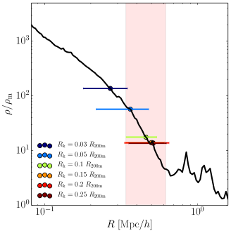
In order for our algorithm to identify the splashback shell reliably, we need to sample the density distribution around the shell well. However, typical densities in this region are $(0.1-10)\times\rho_{\rm m}$ (see Figure 1) and there are often relatively few particles. To compensate for this, we need to make the radius of the spheres associated with particles, $R_{\rm kernel}$ sufficiently large.

To find the optimal value of $R_{\rm kernel}$, we use an approach similar to the approach A above. We generate a representative sample of halos and fit Penna-Dines shells to each halo in the sample for different values of $R_{\rm kernel}$. We then find the smallest converged value of $R_{\rm kernel}$ for each halo. An example of this comparison is shown in Figure 16. This figure also illustrates the second test described in section 3: in ¿99% of cases, $R_{\rm sp}$ falls within the visual fall-off region of the halo.

We find that for halos with $N_{\rm 200m}~{}\geq~{}10^{6}$, properties of the splashback shells converge for $R_{\rm kernel}\gtrsim 0.1R_{\rm 200m}$ and for halos with $N_{\rm 200m}\approx 5\times 10^{4}$ for $R_{\rm kernel}\gtrsim 0.2R_{\rm 200m}$. For simplicity, we set $R_{\rm kernel}$ to $0.2R_{\rm 200m}$ for all halos.

C.2. Setting $N_{\rm planes}$

Figure 16.— Left: Convergence test of $R_{\rm sp}$ as a function of kernel radius for a representative halo. The black curve is the density profile of the halo obtained through conventional particle binning, the points are the $R_{\rm sp}$ values measured from density fields generated with different kernel radii, the horizontal lines show the range spanned by the minimum and maximum radii of these shells, and the shaded red region corresponds to the radial range which was visually identified as corresponding to the splashback range. This region was found by eye without knowledge of the measurements made by Shellfish in accordance with the procedure outlined in section 3. For this halo, $R_{\rm sp}$ is converged for kernel radii above $0.15R_{\rm k}$. Right:The mean fractional stochastic error in shell parameters (defined in Equations 7 - 11) as a function of $N_{\rm planes}$. The vertical dashed line corresponds to $N_{\rm planes}=100$, the value given in Table 2.

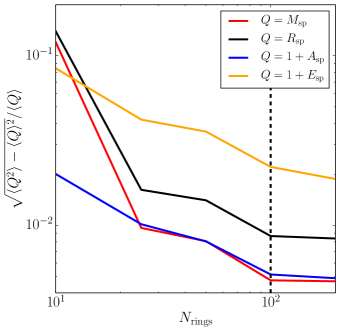
The parameter which has the largest effect on the stochastic error, as opposed to systematic error, in estimating shell shape is $N_{\rm planes}$. To determine a value for this parameter, we follow a procedure similar to method A. We identify the splashback shells for a representative sample of halos for five values of $N_{\rm planes}$, using randomly oriented normal vectors for each plane so that no lines of sight are shared between two different realizations. We then calculate the fractional standard deviation between shell properties determined for different random realizations of a given number of planes $N_{\rm planes}$, $\sqrt{\langle Q^{2}\rangle-\langle Q\rangle^{2}}/\langle Q\rangle$ for each quantity $Q$ defined in Equations 7 - 11. This standard deviation is plotted as a function of $N_{\rm planes}$ in Figure 16. For $N_{\rm planes}=100$, Shellfish achieves sub-percent level per-halo scatter in $R_{\rm sp}$, $M_{\rm sp}$, and $1+A_{\rm sp}$ and less than 2% scatter in $1+E_{\rm sp}$. We do not find any evidence that the amplitudes of the curves shown in Figure 16 depend on halo mass or accretion rate.

Appendix D Computing Moment of Inertia-Equivalent Ellipsoidal Shell Axes

It is non-trivial to analytically compute axis ratios from the moments of inertia for a constant-density ellipsoidal shell. Assuming that the shell is sampled by some collection of particles with weights $m_{k}$, the moments can be obtained by calculating the eigenvalues of the mass-distribution tensor,

$$M_{i,j}=\sum_{k}m_{k}(\vec{r}_{k})_{i}(\vec{r}_{k})_{j}.$$ (D1)

The eigenvalues of the mass-distribution tensor are straightforward to calculate for a homoeoid: the volume enclosed by two ellipsoids with the same axes ratios and with aligned major axes $a$ and $a^{\prime}$. In the limit where $a^{\prime}\rightarrow a$, the eigenvalues are given by

$$M_{i}=M_{\rm tot}\frac{a_{i}^{2}}{3},$$ (D2)

where $M_{i}$ and $a_{i}$ are the moment and ellipsoid axis aligned with the i^th Cartesian axis and $M_{\rm tot}=\sum_{k}m_{k}$. Note that this notation for ellipsoid axes is different that the convention used in Equation 9. Although an infinitely thin homoeoid is often equated with a uniform-density ellipsoid surface in the literature (see, for example Zemp et al., 2011), it actually corresponds to an ellipsoid surface with a non-uniform density. This non-uniformity means that major (minor) axes derived from Equation D2 are too small (large). This bias increases with increasing ellipticity: for ellipsoidal shells with axes ratio of $\approx 2:1$, this can bias measured axes ratios by tens of per cent.

A more accurate approximation would be to model a uniform density ellipsoidal shell by the volume enclosed by two ellipsoids with axes $a$, $b$, $c$ and $a+\delta$, $b+\delta$, $c+\delta$ and to take $\delta\rightarrow 0$. This shape gives eigenvalues of

$$M_{i}=M_{\rm tot}\frac{a_{i}^{2}}{5}\left(\frac{a_{i}a_{j}+3a_{j}a_{k}+a_{k}a_{i}}{a_{i}a_{j}+a_{j}a_{k}+a_{k}a_{i}}\right),$$ (D3)

which can then be numerically solved to obtain ellipsoid axes. Although for ellipsoids with large axes ratios Equation D3 is a closer approximation than Equation D2, it still introduces errors close to our $N_{\rm ring}=100$ stochastic noise limit. Thus for large axes-ratio ellipsoids we compute the mapping empirically.

We define the quantities $A_{i}\equiv\sqrt{M_{i}/M_{\rm tot}}$ and $R\equiv(M_{i}M_{j}M_{k}/M_{\rm tot}^{3})^{1/6}$. Note that both $A_{i}$ and $R$ can be measured directly from the input point distribution. First, we generate a grid of ellipsoids in $a_{0}/a_{1}$ - $a_{0}/a_{2}$ space. Next we numerically compute $A_{0}/A_{1}$, $A_{0}/A_{2}$, and $a_{0}/R_{\rm V}$ for each ellipsoid. The resultant $A_{0}/A_{1}$ and $A_{0}/A_{2}$ values form a sheared grid, so we Delaunay triangulate (Delaunay, 1934) the $A_{0}/A_{1}$ - $A_{0}/A_{2}$ plane and perform linear interpolation on the resulting triangles. We construct three such interpolators which map from ($A_{0}/A_{1}$, $A_{0}/A_{2}$) pairs to $a_{0}/a_{1}$, $a_{0}/a_{2}$, and $a_{0}/R$, respectively. These interpolators can then be used to find $a_{0}$, $a_{1}$, and $a_{2}$ using only the eigenvalues of the mass-distribution tensor.

References

- Abel et al. (2012) Abel, T., Hahn, O., & Kaehler, R. 2012, MNRAS, 427, 61
- Adhikari et al. (2014) Adhikari, S., Dalal, N., & Chamberlain, R. T. 2014, JCAP, 11, 019
- Adhikari et al. (2016) Adhikari, S., Dalal, N., & Clampitt, J. 2016, ArXiv e-prints, arXiv:1605.06688
- Behroozi et al. (2013) Behroozi, P. S., Wechsler, R. H., & Wu, H.-Y. 2013, ApJ, 762, 109
- Behroozi et al. (2013) Behroozi, P. S., Wechsler, R. H., & Wu, H.-Y. 2013, The Astrophysical Journal, 762, 109. http://stacks.iop.org/0004-637X/762/i=2/a=109
- Behroozi et al. (2013) Behroozi, P. S., Wechsler, R. H., Wu, H.-Y., et al. 2013, ApJ, 763, 18
- Bertschinger (1985) Bertschinger, E. 1985, ApJS, 58, 39
- Dalal et al. (2010) Dalal, N., Lithwick, Y., & Kuhlen, M. 2010, ArXiv e-prints, arXiv:1010.2539
- Delaunay (1934) Delaunay, B. 1934, Bulletin de l’Académie des Sciences de l’URSS, Classe des sciences mathématiques et naturelles, 6, 793
- Diemer (2017) Diemer, B. 2017, ArXiv e-prints, arXiv:1703.09712
- Diemer & Kravtsov (2014) Diemer, B., & Kravtsov, A. V. 2014, ApJ, 789, 1
- Diemer et al. (2013a) Diemer, B., Kravtsov, A. V., & More, S. 2013a, ApJ, 779, 159
- Diemer et al. (2017) Diemer, B., Mansfield, P., Kravtsov, A. V., & More, S. 2017, ArXiv e-prints, arXiv:1703.09716
- Diemer et al. (2013b) Diemer, B., More, S., & Kravtsov, A. V. 2013b, ApJ, 766, 25
- Fillmore & Goldreich (1984) Fillmore, J. A., & Goldreich, P. 1984, ApJ, 281, 1
- Goodman & Weare (2010) Goodman, J., & Weare, J. 2010, Communications in Applied Mathematics and Computational Science, 5, 65
- Górski et al. (2005) Górski, K. M., Hivon, E., Banday, A. J., et al. 2005, ApJ, 622, 759
- Gringorten & Yepez (1992) Gringorten, I. I., & Yepez, P. J. 1992, Instrumentation Papers, 343, 1
- Gunn & Gott (1972) Gunn, J. E., & Gott, III, J. R. 1972, ApJ, 176, 1
- Hahn & Angulo (2016) Hahn, O., & Angulo, R. E. 2016, MNRAS, 455, 1115
- Heath (1977) Heath, D. J. 1977, MNRAS, 179, 351
- Jing & Suto (2002) Jing, Y. P., & Suto, Y. 2002, ApJ, 574, 538
- Kazantzidis et al. (2006) Kazantzidis, S., Zentner, A. R., & Kravtsov, A. V. 2006, ApJ, 641, 647
- Klypin et al. (2011) Klypin, A. A., Trujillo-Gomez, S., & Primack, J. 2011, ApJ, 740, 102
- Komatsu et al. (2011) Komatsu, E., Smith, K. M., Dunkley, J., et al. 2011, ApJS, 192, 18
- Kravtsov & Borgani (2012) Kravtsov, A. V., & Borgani, S. 2012, ARA&A, 50, 353
- Lahav et al. (1991) Lahav, O., Lilje, P. B., Primack, J. R., & Rees, M. J. 1991, MNRAS, 251, 128
- Mansfield et al. (2017) Mansfield, P., Kravtsov, A., & Diemer, B. 2017, phil-mansfield/shellfish: AAS Release, , , doi:10.5281/zenodo.546241. https://doi.org/10.5281/zenodo.546241
- More et al. (2015) More, S., Diemer, B., & Kravtsov, A. V. 2015, ApJ, 810, 36
- More et al. (2016) More, S., Miyatake, H., Takada, M., et al. 2016, ArXiv e-prints, arXiv:1601.06063
- Patej & Loeb (2016) Patej, A., & Loeb, A. 2016, ApJ, 824, 69
- Penna & Dines (2007) Penna, M. A., & Dines, K. A. 2007, IEEE Transactions on Pattern Analysis and Machine Intelligence, 29, 1673
- Powell & Abel (2014) Powell, D., & Abel, T. 2014, ArXiv e-prints, arXiv:1412.4941
- Rines et al. (2013) Rines, K., Geller, M. J., Diaferio, A., & Kurtz, M. J. 2013, ApJ, 767, 15
- Savitzky & Golay (1964) Savitzky, A., & Golay, M. J. E. 1964, Analytical Chemistry, 36, 1627
- Shi (2016) Shi, X. 2016, MNRAS, 459, 3711
- Springel (2005) Springel, V. 2005, MNRAS, 364, 1105
- Sunayama et al. (2016) Sunayama, T., Hearin, A. P., Padmanabhan, N., & Leauthaud, A. 2016, MNRAS, 458, 1510
- Tolman (1934) Tolman, R. C. 1934, Proceedings of the National Academy of Science, 20, 169
- Tully (2015) Tully, R. B. 2015, AJ, 149, 54
- Umetsu & Diemer (2017) Umetsu, K., & Diemer, B. 2017, ApJ, 836, 231
- Wang et al. (2009) Wang, H., Mo, H. J., & Jing, Y. P. 2009, MNRAS, 396, 2249
- Wetzel et al. (2014) Wetzel, A. R., Tinker, J. L., Conroy, C., & van den Bosch, F. C. 2014, MNRAS, 439, 2687
- Zemp et al. (2011) Zemp, M., Gnedin, O. Y., Gnedin, N. Y., & Kravtsov, A. V. 2011, ApJS, 197, 30
- Zentner et al. (2016) Zentner, A. R., Hearin, A., van den Bosch, F. C., Lange, J. U., & Villarreal, A. 2016, ArXiv e-prints, arXiv:1606.07817
- Zhuravleva et al. (2013) Zhuravleva, I., Churazov, E., Kravtsov, A., et al. 2013, MNRAS, 428, 3274